Formation of Raman Scattering Wings around H$\alpha$, H$\beta$ and Pa$\alpha$ in Active Galactic Nuclei

Abstract

Powered by a supermassive black hole with an accretion disk, the spectra of active galactic nuclei (AGNs) are characterized by prominent emission lines including Balmer lines. The unification schemes of AGNs require the existence of a thick molecular torus that may hide the broad emission line region from the view of observers near the equatorial direction. In this configuration, one may expect that the far UV radiation from the central engine can be Raman scattered by neutral hydrogen to reappear around Balmer and Paschen emission lines which can be identified with broad wings. We produce H$\alpha$, H$\beta$ and Pa$\alpha$ wings using a Monte Carlo technique to investigate their properties. The neutral scattering region is assumed to be a cylindrical torus specified by the inner and outer radii and the height. While the covering factor of the scattering region affects the overall strengths of the wings, the wing widths are primarily dependent on the neutral hydrogen column density $N_{\rm HI}$ being roughly proportional to $N_{\rm HI}^{1/2}$. In particular, with $N_{\rm HI}=10^{23}{\rm\ cm^{-2}}$ the H$\alpha$ wings typically show a width $\sim 2\times 10^{4}{\rm\ km\ s^{-1}}$. We also find that H$\alpha$ and Pa$\alpha$ wing profiles are asymmetric with the red part stronger than the blue part and an opposite behavior is seen for H$\beta$ wings.

1. Introduction

Active galactic nuclei (AGNs) are known to be powered by a supermassive black hole with an accretion disk. The spectra of AGNs are characterized by a nonthermal featureless continuum with prominent emission lines exhibiting a large range of ionization and excitation (e.g., Peterson, 1997). One classification of AGNs can be made based on the width of emission lines. Type 1 AGNs show broad permitted lines and semi-forbidden lines with a typical width of $5,000{\rm\ km\ s^{-1}}$. In addition to these broad emission lines they also show narrow forbidden lines with a width $\sim 500{\rm\ km\ s^{-1}}$. In contrast to this, type 2 AGNs exhibit only narrow emission lines encompassing both permitted and forbidden lines.

Blandford & McKee (1982) proposed that the location of the broad line region can be observationally constrained by monitoring the flux of emission lines that vary in response to the changes of continuum flux. The time delay is directly translated into the size of the broad emission line region, which is also used to estimate the mass of the black hole (e.g., Bentz et al., 2009; Park et al., 2012). The reverberation mapping shows that the broad emission line region is located within $\sim 0.1{\rm\ pc}$ from the central engine, whereas the narrow emission lines do not exhibit flux variations correlated with the neighboring continuum (e.g., Peterson, 1993; Dietrich et al., 2012). A typical AGN unification model proposes that an optically and geometrically thick component resides between the broad emission line region and the narrow emission line region, hindering the observers in the equatorial direction from viewing the broad line region.

Spectropolarimetry can be an efficient tool to verify this unification scheme, because we expect the broad emission lines may be seen in the polarized spectra in the presence of a scattering medium in the polar direction (e.g., Antonucci, 1993). The prototypical type 2 Seyfert galaxy, NGC 1068, shows broad Balmer lines in the polarized flux (e.g., Antonucci & Miller, 1985). A similar observation was made for the narrow line radio galaxy Cyg A by Ogle et al. (1997), in which an extremely broad H$\alpha$ line was found in the polarized flux.

Broad absorption line quasars (BALQs), constituting about 10 percent of quasars, exhibit broad absorption troughs in the blue part of permitted broad lines. The exact nature of the absorbing media being controversial, one suggestion is that broad absorption lines are formed in the equatorial outflow that is driven radiatively by quasar luminosity (e.g., Murray & Chiang, 1995). In this case the broad troughs will not be completely black but filled partially by photons resonantly scattered in other lines of sight (e.q., Lee & Blandford, 1997). Spectropolarimetry is also applied to find polarized residual fluxes in the broad absorption troughs in a number of BALQs (e.g., Cohen et al., 1995).

In the presence of an optically thick component, it is expected that far UV radiation can be inelastically scattered by neutral hydrogen, which may result in scattered radiation in the visible and IR regions. Raman scattering by atomic hydrogen was first introduced by Schmid (1989), when he identified the broad features around $6825\,{\rm\AA}$ and $7082\,{\rm\AA}$. These mysterious broad features are found in about half of symbiotic stars, wide binary systems consisting of an active white dwarf and a mass losing giant (e.q., Kenyon, 1986). The broad 6825 and 7082 emission features are formed through Raman scattering of O VI$\lambda\lambda$1032 and 1038, when the scattering hydrogen atom in the ground state before incidence finally de-excites to the $2s$ state.

The cross sections of Raman scattering for O VI$\lambda\lambda$1032 and 1038 are $6.6\sigma_{Th}$ and $2.0\sigma_{Th}$, respectively, where $\sigma_{Th}=0.665\times 10^{-24}{\rm\ cm^{2}}$ is the Thomson scattering cross section. Due to the small scattering cross section, the operation of Raman scattering by atomic hydrogen requires a large amount of neutral hydrogen that is illuminated by the far UV emission source. However, the cross section increases sharply as the incident wavelength approaches those of Lyman series transition of hydrogen due to resonance.

The energy conservation requires the wavelength $\lambda_{o}$ of the Raman scattered radiation to be related to the incident wavelength $\lambda_{i}$ by

$$\lambda_{o}^{-1}=\lambda_{i}^{-1}-\lambda_{\alpha}^{-1},$$ (1)

where $\lambda_{\alpha}$ is the wavelength of Ly$\alpha$. This relation immediately leads to the following

$${\Delta\lambda_{o}\over\lambda_{o}}={\lambda_{o}\over\lambda_{i}}{\Delta\lambda_{i}\over\lambda_{i}},$$ (2)

which dictates that the Raman features have a large width broadened by the factor $\lambda_{o}/\lambda_{i}$. In the case of Raman scattering of O VI$\lambda$1032, $\lambda_{o}/\lambda_{i}\simeq 6.6$ which explains the abnormally broad width exhibited in the Raman O VI$\lambda$6825 feature.

In a similar way, Raman scattering of continuum photons in the vicinity of Ly$\beta$ may form broad features around H$\alpha$. This mechanism has been invoked to explain broad H$\alpha$ wings prevalent in symbiotic stars (Lee, 2000; Yoo et al., 2002). Lee & Yun (1998) also discussed polarized H$\alpha$ through Raman scattering in active galactic nuclei, where neutral regions may be thicker than those found in symbiotic stars.

The next section provides summary of the atomic physics involving Raman scattering by atomic hydrogen. Subsequently we provide our model for computation of broad Balmer and Paschen wings with our simulated results. A brief discussion is provided before conclusion.

2. Atomic Physics of Raman Scattering by H I

The exact nature of the thick absorbing component surrounding the broad emission line region in AGNs is still controversial. X-ray observation can be an excellent tool to probe the physical properties of the intrinsic absorber in AGNs. One such study performed using Suzaku by Chiang et al. (2013) reported the column density of hydrogen $N_{\rm HI}\sim 5\times 10^{23}{\rm\ cm^{-2}}$ in the type 2 quasar IRAS 09104+4109. In the presence of this thick neutral hydrogen, the Rayleigh and Raman scattering optical depth for radiation in the vicinity Lyman series can be quite significant.

The scattering of light by an atomic electron is described by the second order time dependent perturbation theory. We consider an incident photon with angular frequency $\omega$ with the polarization vector ${\boldsymbol{\epsilon}}^{\alpha}$ scattered by an electron in the initial state $A$, which subsequently de-excites to the final state $B$ accompanied by the emission of an outgoing photon with angular frequency $\omega^{\prime}$ with polarization vector ${\boldsymbol{\epsilon}}^{\alpha^{\prime}}$. The energy conservation requires that the difference of the photon energy

$$\hbar(\omega-\omega^{\prime})=E_{B}-E_{A},$$ (3)

where $E_{A}$ and $E_{B}$ are the energy of the initial and final states $A$ and $B$, respectively.

Depending on the sign of $E_{B}-E_{A}$, the emergent Raman lines are classified into Stokes and anti-Stokes lines. When $E_{B}-E_{A}>0$, we have a Stokes line, which is less energetic than the incident radiation. If $E_{B}-E_{A}<0$, then the transition corresponds to an anti-Stokes line. In this work, all the transitions correspond to Stokes lines.

In this work, no consideration is made of the polarization of Raman wings, which is deferred to a future work.

The cross section for this interaction is given by the Kramers-Heisenberg formula

$${d\sigma\over d\Omega} = r_{0}^{2}\left({\omega^{\prime}\over\omega}\right)\left|\delta_{AB}{{\boldsymbol{\epsilon}}^{\alpha}}\cdot{{\boldsymbol{\epsilon}}^{\alpha^{\prime}}}\right.$$ (4)

$$- {1\over m_{e}\hbar}\sum_{I}\left({{({\bf p}\cdot{\boldsymbol{\epsilon}}^{(\alpha^{\prime})})_{BI}({\bf p}\cdot{\boldsymbol{\epsilon}}^{(\alpha)})_{IA}}\over{\omega_{IA}-\omega}}\right.$$

$$- \left.\left.{{({\bf p}\cdot{\boldsymbol{\epsilon}}^{(\alpha)})_{BI}({\bf p}\cdot{\boldsymbol{\epsilon}}^{(\alpha^{\prime})})_{IA}}\over{\omega_{IA}+\omega^{\prime}}}\right)\right|^{2},$$

where $\omega_{IA}=\omega_{I}-\omega_{A}=(E_{I}-E_{A})/\hbar$ is the angular frequency corresponding to the intermediate state $I$ and the initial state $A$ (e.g. Sakurai 1967). The intermediate state $I$ covers all the bound states $np$ and free states $n^{\prime}p$, where $n^{\prime}$ is the positive real number. Here, $r_{0}=e^{2}/(m_{e}c^{2})=2.82\times 10^{-13}{\rm\ cm}$ is the classical electron radius with $m_{e}$ and $e$ being the electron mass and charge. Note that the summation in the formula consists of a summation over infinitely many $np$ states and an integral over continuous free states $n^{\prime}p$. Adopting the atomic units where $\hbar=e=m_{e}=1$, we note that

$$E_{n}=\omega_{n}=-{1\over 2n^{2}}$$ (5)

for a bound state $np$ and

$$E_{n}^{\prime}=\omega_{n^{\prime}}={1\over 2n^{\prime 2}}$$ (6)

for a free state $n^{\prime}p$.

In this work, we make no consideration on the polarization of Raman wings, which is deferred to a future work. The averaging over the solid angle and polarization states yields a numerical factor of $8\pi/3$, leading to the Thomson cross section $\sigma_{Th}=8\pi r_{0}^{2}/3$. In the case of Rayleigh scattering, for which the initial and the final states are the same, the cross section can be re-written as

$$\sigma_{Ray}(\omega) = \sigma_{Th}\left|\sum_{I}\left({{\omega<p>_{IA}<p>_{AI}}\over{\omega_{IA}-\omega}}\right.\right.$$ (7)

$$- \left.\left.{{\omega<p>_{IA}<p>_{AI}}\over{\omega_{IA}+\omega}}\right)\right|^{2}$$

(e.g. Sakurai 1967, Bach & Lee 2014).

The bound state radial wavefunction is written as

$$R_{nl}(r) = {2\over n^{l+2}(2l+1)!}\left[{(n+l)!\over(n-l-1)!}\right]^{1/2}(2r)^{l}e^{-r/n}$$ (8)

$$\times F(-n+l+1,2l+2,2r/n),$$

where $F(\alpha,\beta,z)$ is the hypergeometric function defined by

$$F(\alpha,\beta,z)=1+{\alpha\over\beta}{z\over 1!}+{\alpha(\alpha+1)\over\beta(\beta+1)}{z^{2}\over 2!}+\cdots.$$ (9)

For a free state $|n^{\prime}l>$, the radial wavefunction is written as

$$\hskip-15.0ptR_{n^{\prime}l}(r)={2n^{\prime 1/2}\over[1-e^{-2\pi n^{\prime}}]^{1/2}(2l+1)!}\prod_{s=1}^{l}\left(1+{s^{2}\over n^{\prime 2}}\right)^{1/2}$$

$$\hskip-10.0pt\times(2r)^{l}e^{-ir/n^{\prime}}F(in^{\prime}+l+1,2l+2,2ir/n^{\prime})$$ (10)

with the normalization condition

$$\int_{0}^{\infty}R_{n^{\prime}l}(r)R_{n^{\prime\prime}l}(r)r^{2}dr=\delta(n^{\prime}-n^{\prime\prime})$$ (11)

(e.g. Bethe & Salpeter 1957, Saslow & Mills 1969).

With these expressions of the radial wavefunctions the explicit expression for relevant matrix elements between the $1s$ state and an $np$ bound state is given by

$$<np|p|1s>=-i\left[{2^{6}n^{3}(n-1)^{2n-3}\over(n+1)^{2n+3}}\right]^{1/2}.$$ (12)

Between a free $n^{\prime}p$ state and the ground $1s$ state the matrix element is given by

$$<n^{\prime}p|p|1s>=-i\left[{2^{6}n^{\prime 3}(1-e^{-2\pi n^{\prime}})^{1/2}}\over(n^{\prime 2}+1)^{3}e^{2n^{\prime}\tan^{-1}(1/n^{\prime})}\right]^{1/2}.$$ (13)

In the case of Raman scattering where $A\neq B$, the Kronecker delta term vanishes in Eq.(4) leaving the two summation terms which contribute to the cross section. The relevant matrix elements are $<np|p|2s>,<np|p|3s>$ and $<np|p|3d>$ and their free state counterparts, which are listed in Table 1.

Table 1Matrix elements of the momentum operator $p$ in atomic units.

Matrix	Element
$<2s|p|np>\ =$	$-i32\sqrt{2}n^{3/2}(n^{2}-1)^{1/2}(n^{2}-4)^{-2}[(n-2)/(n+2)]^{n}$
$<2s|p|n^{\prime}p>\ =$	$-i32\sqrt{2}n^{\prime 3/2}(n^{\prime 2}+1)^{1/2}(n^{\prime 2}+4)^{-2}(1-e^{-2\pi n^{\prime}})^{-1/2}e^{-2n^{\prime}\tan^{-1}(2/n^{\prime})}$
$<3s|p|np>\ =$	$-i24\sqrt{3}n^{3/2}(n^{2}-1)^{1/2}(17n^{2}-27)(n^{2}-9)^{-3}[(n-3)/(n+3)]^{n}$
$<3s|p|n^{\prime}p>\ =$	$-i24\sqrt{3}n^{\prime 3/2}(1+n^{\prime 2})^{1/2}(7n^{\prime 2}+27)(1-e^{-2\pi n^{\prime}})^{-1/2}(n^{\prime 2}+9)^{-3}e^{-2n^{\prime}\tan^{-1}(3/n^{\prime})}$
$<3d|p|np>\ =$	$-i96\sqrt{3}n^{11/2}(n^{2}-1)^{1/2}(n^{2}-9)^{-3}[(n-3)/(n+3)]^{n}$
$<3d|p|n^{\prime}p>\ =$	$-i96\sqrt{3}n^{\prime 11/2}(1+n^{\prime 2})^{1/2}(1-e^{-2\pi n^{\prime}})^{-1/2}(n^{\prime 2}+9)^{-3}e^{-2n^{\prime}\tan^{-1}(3/n^{\prime})}$

The total scattering cross section $\sigma_{\rm tot}$ is given by the sum of the Rayleigh and Raman scattering cross sections. The number of Raman scattering branching channels differs depending on the frequency of the incident photon. For example, the final states of H I for incident photons blueward of Ly$\beta$ may include $1s$, $2s$, $3s$ and $3d$ states, whereas only $1s$ and $2s$ states can be the final state for those redward of Ly$\beta$ and blueward of Ly$\alpha$.

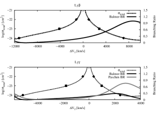
Figure 1.— Total scattering cross section and branching ratios around Ly$\beta$ (upper panel) and Ly$\gamma$ (lower panel). The solid lines are the sum of cross sections of Rayleigh scattering and Raman scattering. The dotted lines are the branching ratio of scattering into the $2s$ state and the thin gray line shows the branching ratio into the $n=3$ levels. Note that for $\lambda\geq 974.48{\rm\ \AA}$ the branching ratio into $n=3$ is larger than that into $n=2$.

In Fig. 1, we show the total scattering cross section $\sigma_{\rm tot}$ by a dotted line. We also show the branching ratio into $2s$ by a thick solid line and the branching ratio into $n=3$ states yielding Pa$\alpha$ wings by a thin gray line. We define the Doppler velocity factor $\Delta V_{1}$ around Ly$\beta$ by

$${{\Delta V_{1}}}={{\lambda-\lambda_{\beta}}\over\lambda_{\beta}}c$$ (14)

where $\lambda_{\beta}$ is the wavelength of Ly$\beta$. In terms of $\Delta V_{1}$ we find the total scattering cross section exceeding $10^{-22}{\rm\ cm^{2}}$ in the range $-1,264{\rm\ km\ s^{-1}}<\Delta V_{1}<+930{\rm\ km\ s^{-1}}$. As Lee (2013) pointed out the total cross section is stronger in the blue side than the red side around Ly$\beta$. The range of $\Delta V_{1}$ corresponding to $\sigma_{\rm tot}\geq 10^{-23}{\rm\ cm^{2}}$ is $-4,162{\rm\ km\ s^{-1}}<\Delta V_{1}<+2,805{\rm\ km\ s^{-1}}$.

In a similar way, we introduce the Doppler factor $\Delta V_{2}$ defined as

$${{\Delta V_{2}}}={{\lambda-\lambda_{\gamma}}\over\lambda_{\gamma}}c$$ (15)

where $\lambda_{\gamma}$ is the wavelength of Ly$\gamma$. For radiation in the vicinity of Ly$\gamma$ the velocity range for $\sigma_{\rm tot}\geq 10^{-22}{\rm\ cm^{2}}$ is given by $-553{\rm\ km\ s^{-1}}<\Delta V_{2}<281{\rm\ km\ s^{-1}}$. When we increase the column density to $N_{\rm HI}=10^{23}{\rm\ cm^{-2}}$, the velocity range corresponding to the total optical depths exceeding unity is $-1,809{\rm\ km\ s^{-1}}<\Delta V_{2}<+934{\rm\ km\ s^{-1}}$. In the vicinity of Ly$\gamma$, the total cross sections are also asymmetric showing larger values in the blue part than in the red part. This trend is similar to that around Ly$\beta$. Furthermore, the branching ratio of scattering into the $2s$ state is also increasing as a function of the wavelength. In particular, the branching ratio into $n=3$ in Fig. 1 is larger than that into $n=2$ for $\lambda\geq 974.48{\rm\ \AA}$. This implies that in the red part of Ly$\gamma$ with incident wavelength $\lambda\geq 974.48{\rm\ \AA}$ we expect more Raman scattered photons redward of Pa$\alpha$ than those redward of H$\beta$.

In Table 2 we summarize these values for neutral column densities ranging from $10^{22}{\rm\ cm^{-2}}$ to $10^{24}{\rm\ cm^{-2}}$. As is shown in the table, the velocity widths are significantly larger around Ly$\beta$ than around Ly$\gamma$. The Raman wing width is obtained roughly from this width in the parent wavelength space multiplied by the numerical factor $(\lambda_{o}/\lambda_{i})^{2}$ due to the inelasticity of scattering. The latter factor is the largest for Pa$\alpha$ wings and smallest for H$\beta$ wings. From this we may expect that the extent of H$\beta$ wings will be much smaller than that of Pa$\alpha$ wings. The branching ratio into $n=3$ states being comparable to that into $n=2$ around Ly$\gamma$, the Pa$\alpha$ wings will be much broader but shallower than the H$\beta$ counterparts.

The total scattering optical depth of unity for $N_{\rm HI}=10^{23}{\rm\ cm^{-2}}$ is obtained for incident radiation with wavelengths $\lambda_{\beta 1}=1011.83{\rm\ \AA}$, $\lambda_{\beta 2}=1035.69{\rm\ \AA}$ around Ly$\beta$. These photons are Raman scattered to appear at $6047{\rm\ \AA}$, and $7012{\rm\ \AA}$ around H$\alpha$.

In a similar way, we have the total scattering optical depth of unity at $\lambda_{\gamma 1}=966.99{\rm\ \AA}$, $\lambda_{\gamma 2}=975.90{\rm\ \AA}$ around Ly$\gamma$, for which Raman scattered features reappear at $4735{\rm\ \AA}$ and $4956{\rm\ \AA}$ around H$\beta$ and at $16890{\rm\ \AA}$ and $20090{\rm\ \AA}$ around Pa$\alpha$.

$N_{\rm HI}$	$\lambda_{1}$	$\Delta V_{1}$	$\lambda_{2}$	$\Delta V_{2}$
$[{\rm cm^{-2}}]$	$[{\rm\ \AA}]$	$[{\rm km\ s^{-1}}]$	$[{\rm\ \AA}]$	$[{\rm km\ s^{-1}}]$
$10^{22}$	$1021.75,\ 1029.27$	$-1264,\ +930$	$971.07,\ 973.78$	$-553,\ +281$
$10^{22.5}$	$1018.37,\ 1031.76$	$-2253,\ +1657$	$969.74,\ 974.62$	$-960,\ +539$
$10^{23}$	$1011.83,\ 1035.69$	$-4162,\ +2805$	$966.99,\ 975.90$	$-1809,\ +934$
$10^{23.5}$	$1000.30,\ 1041.51$	$-7530,\ +4506$	$961.69,\ 977.75$	$-3443,\ +1505$
$10^{24}$	$987.68,\ 1050.29$	$-11218,\ +7069$	$956.14,\ 980.74$	$-5151,\ +2427$

Table 2Wavelengths and the corresponding Doppler factors having a unit total scattering optical depth for various values of neutral hydrogen column density $N_{\rm HI}$. The two values of $\lambda_{1}$ and those of $\lambda_{2}$ are wavelengths around Ly$\beta$ and Ly$\gamma$, respectively. The Doppler factors $\Delta V_{1}$ and $\Delta V_{2}$ are defined by Eq. (14) and Eq. (15), respectively.

3. Monte Carlo Radiative Transfer

We consider a neutral scattering region as a finite cylinder characterized by the thickness and the height. The symmetry axis is chosen to be $z$ axis and the AGN continuum source is assumed to reside at the center of the coordinate system.

The AGN continuum is known to be nonthermal and typically approximated by a power law (e.g., Zheng al., 1997; Vanden Berk et al., 2001). It also appears that far UV continuum spectrum around Ly$\beta$ and Ly$\gamma$ is almost flat in many AGNs. In this respect the continuum considered in this work is described by

$$\lambda F_{\lambda}=\lambda_{0}F_{0}\left({\lambda\over\lambda_{0}}\right)^{\alpha},$$ (16)

where the spectral index $\alpha$ is set to zero in this work, and $\lambda_{0}$ is a characteristic wavelength in this spectral region.

Spectropolarimetry of the prototypical Seyfert 2 galaxy NGC 1068 performed by Antonucci & Miller (1985) shows that H$\beta$ appears broad in the polarized flux. This implies that NGC 1068 possesses the broad line region that is hidden from the observer’s line of sight by an optically thick torus-like region. Almost constant position angle in the polarized flux is consistent with the scattering region located in the polar direction with respect to the central engine.

In performing our simulations it is assumed that the far UV incident radiation does not affect the physical and chemical conditions of the neutral scattering region. With this assumption, the Rayleigh-Raman radiative transfer of far UV continuum can be divided coceptually into radiative transfer of each individual photon with a definite frequency that constitutes the whole far UV continuum.

Compared with usual Raman spectroscopy performed in a lab with a monochromatic laser with a definite polarization state, our simulation of Raman scattering by atomic hydrogen in AGN differs mainly in our neglect of polarization. As far as no measurement is made of the polarization of the final emergent photon, the radiative transfer using Eq. (7) for unpolarized light is equivalent to obtaining the total number flux of Raman scattered radiation from simulations that take a full consideration of polarization. With these limitations noted, we simulate the Raman wing formation by injecting an unpolarized individual photon with a definite frequency. The number of these photons is determined in an accordance of AGN comtinuum spectrum.

Additional information regarding the existence of the optically thick component can be obtained from studies of X-ray hardness of AGNs. Because soft X-rays suffer more severe extinction than hard X-rays, type 2 AGNs tend to exhibit larger X-ray hardness than type 1 AGNs. X-ray studies show that the optically thick component is characterized by a hydrogen column density ranging $10^{22-24}{\rm\ cm^{-2}}$.

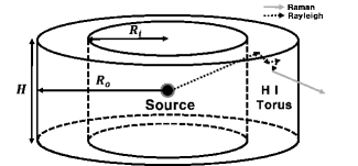
Figure 2.— Scattering geometry of AGNs, where the neutral scattering region is considered to be a cylindrical torus with $R_{i}$, $R_{o}$ and $H$ being the inner radius, outer radius and the height.

In this work we place an optically thick component in the form of a cylindrical torus with a finite height, which is schematically shown in Fig. 2. This torus is specified by the inner radius $R_{i}$, the outer radius $R_{o}$ and the height $H$. For the sake of simplicity, we fix the thickness of the torus $\Delta R=R_{o}-R_{i}=10\,{\rm pc}$ and we assume that the number density of neutral hydrogen $n_{\rm HI}$ is uniform in the scattering region. In this case, the scattering region can be specified by the lateral column density $N_{\rm HI}=n_{\rm HI}\Delta R$. The height $H$ is parameterized by $A=H/\Delta R$, the ratio of the height and the thickness $\Delta R$. In this work, we vary $A$ between 0.5 and 2 and also consider $N_{\rm HI}$ in the range $10^{22-24}{\rm\ cm^{-2}}$.

The Monte Carlo simulation starts with the generation of a far UV continuum photon from the central engine, which subsequently enters the scattering region. The wavelength of the incident photon is determined in accordance with the power law of the AGN continuum given in Eq. (16). For this wavelength we rescale the scattering geometry in terms of the total scattering optical depths $\tau_{R}=\sigma(\lambda)n_{\rm HI}\Delta R$ and $\tau_{H}=\sigma(\lambda)n_{\rm HI}H$.

To determine the first scattering site we compute the optical depth $\tau$ for this photon given by

$$\tau=-\ln R,$$ (17)

where $R$ is a random number uniformly distributed in the interval [0,1].

According to the branching ratio we determine the scattering type. If the scattering is Rayleigh, then we look for the next scattering site by taking another step given by Eq. (17). If the branching is into $n=2$ or $n=3$ states, then we have a Raman scattered photon which is supposed to escape from the region immediately. Both Rayleigh scattering and Raman scattering share the scattering phase function which is also identical with that of the Thomson scattering and therefore we choose the direction of the scattered photon in accordance with the Thomson phase function (e.g., Yoo et al., 2002; Schmid, 1989; Nussbaumer et al., 1989).

The collection of Raman scattered photons emergent from the neutral region is made by taking into consideration the difference between the observed wavelength space and the parent far UV wavelength space. The Raman wavelength interval $\Delta\lambda_{o}$ corresponding to a fixed wavelength interval $\Delta\lambda_{i}$ of the incident radiation varies with $\lambda_{i}$ in accordance with Eq. (2). In terms of $\lambda_{i}$ this relation can be recast in the form

$$w_{\lambda_{o}}(\lambda_{i})={\Delta\lambda_{i}\over\Delta\lambda_{o}}=\left({1-{\lambda_{i}\over\lambda_{\alpha}}}\right)^{2}.$$ (18)

This is the factor that relates the number flux per unit wavelength in the parent wavelength space to that in the observed (Raman scattered) wavelength space, which is multiplied to the Monte Carlo simulated flux for proper normalization.

4. Monte Carlo Simulated Raman Wings

4.1. Balmer and Paschen Wings Formed through Raman Scattering

Figure 3.— Monte Carlo simulated profiles of Raman scattered radiation. The upper panel show the Raman scattering wings around H$\alpha$, H$\beta$ and Pa$\alpha$ (upper, middle and bottom panel, respectively). The neutral scattering region is assumed to be a slab with finite thickness and infinite lateral dimensions. The far UV source is located in the midplane.

In Fig. 3, we show the Monte Carlo simulated wings around H$\alpha$, H$\beta$ and Pa$\alpha$ formed through Raman scattering of far UV radiation from the central engine. The parameters associated with the scattering region are $\Delta R=10\ {\rm pc}$ and $H=\infty$, so that the far UV source is immersed at the center of a cylinder with an infinite height. This choice of $H=\infty$ allows us to study the basic properties of Raman wings without complicating effects due to finite covering factors.

We set the neutral hydrogen column density $N_{HI}=n_{HI}\Delta R=10^{23}{\rm\ cm^{-2}}$ in this figure. In this simulation, $10^{4}$ photons are generated per parent wavelength interval of $1{\rm\ \AA}$. The horizontal axis represents the observed wavelength. The vertical axis represents the number of photons obtained in the simulation per unit observed wavelength interval $\Delta\lambda_{o}$.

The profiles of Raman scattered radiation are characterized by the inclined central core part and extended wing part that declines to zero. The inclined central part is formed from far UV photons with the total scattering optical depth exceeding $\sim 10$. Roughly speaking, all the far UV photons within these ranges undergo multiple Rayleigh scattering processes before being converted to optical photons around the Balmer emission centers or IR photons around Pa$\alpha$. The Raman number flux near H$\alpha$ core decreases redward due to the wavelength space factor given in Eq. (18), which is a decreasing function of $\lambda_{i}$. The Raman flux around H$\beta$ shows more steeply inclined core part than that around H$\alpha$. This is explained by the fact that as $\lambda_{i}$ increases the number of photons channeled into the Pa$\alpha$ branch increases very steeply reducing the H$\beta$ flux.

However, far UV photons outside these ranges will be scattered at most once to escape from the scattering region either as far UV photons or as Raman scattered photons. For incident far UV radiation with small scattering optical depths the resultant wing profile will be approximately proportional to the product of the total optical depth and the branching ratio, which is in turn approximately given by the Lorentzian. As Lee (2013) pointed out, the cross section and the branching ratios are complicated functions of wavelength, for which a quantitative investigation can be effectively performed adapting a Monte Carlo technique.

In Fig. 4, we transform the same Monte Carlo data given in Fig. 3 to the parent wavelength space in order to check easily the fraction of Raman scattered photons with respect to the incident radiation. The horizontal dotted line show the incident flux taken to be $10^{4}$ photons per unit wavelength interval. The top panel shows the number of Raman scattered radiation around H$\alpha$. The core part is flat and coincides with the incident flux, which verifies that the Raman conversion is almost complete.

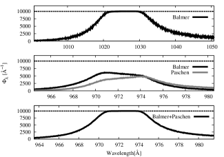
Figure 4.— Monte Carlo simulated profiles of Raman scattered radiation in the parent wavelength space. The horizontal dotted line shows the incident flux taken to be $10^{4}$ photons per unit wavelength interval. The top panel shows the Raman scattered radiation around Ly$\beta$ which shows flat core part because of the complete Raman conversion of the flat incident radiation. The mid panel shows the Raman scattered profiles that appear near H$\beta$ (black lines) and near Pa$\alpha$ (gray lines) from the flat UV radiation near Ly$\gamma$. The bottom panel shows the sum of Raman scattered fluxes around H$\beta$ and Pa$\alpha$ transformed into the parent wavelength space .

The mid panel shows Raman scattered H$\beta$ and Pa$\alpha$ wings by a black solid line and a gray solid line, respectively. The bottom panel shows the sum of Raman scattered H$\beta$ and Pa$\alpha$, where we recover the flat core part coinciding with the incident radiation. This fact provides confirmation that the Raman conversion is also complete in the vicinity of the Ly$\gamma$ core. In this figure, it can be seen that more Pa$\alpha$ wing photons are obtained than H$\beta$ wing photons for incident wavelength $\lambda>974.48{\rm\ \AA}$, where the branching ratio into $n=3$ states exceeds that into the $2s$ state.

4.2. Asymmetry of Raman Scattering Wings

$N_{\rm HI}\,$	$\eta_{\rm H\alpha}$	$\eta_{\rm H\beta}$	$\eta_{\rm Pa\alpha}$
$\rm cm^{-2}$
$10^{22}$	$0.86$	$1.13$	$0.86$
$10^{22.5}$	$0.81$	$1.21$	$0.79$
$10^{23}$	$0.73$	$1.35$	$0.69$
$10^{23.5}$	$0.59$	$1.57$	$0.55$
$10^{24}$	$0.36$	$1.76$	$0.37$

Table 3 The ratio $\eta$ of the Raman photon number flux blueward of line center to that redward of line center in Fig. 3.

In this subsection, we quantify the asymmetry in the wing profiles formed through Raman scattering around H$\alpha$, H$\beta$ and Pa$\alpha$. One way to do this is to compute the ratio $\eta$ of the number of Raman photons blueward of line center to that redward of line center. In Table 3 we show our result.

In the case of H$\alpha$, the red wing part extends further away from the H$\alpha$ center than the blue wing, which is clearly seen by the fact that $\eta_{\rm H\alpha}$ is less than 1. This phenomenon is mainly due to the higher branching ratio for photons redward of Ly$\beta$ than their blue counterparts. A similar behavior is also observed for the Pa$\alpha$ wings due to increasing branching ratio redward of Ly$\gamma$.

However, in the case of H$\beta$ we note that $\eta_{\rm H\beta}$ exceeds unity implying that the blue wing is stronger than the red part. This behavior is attributed to the much stronger total cross section in the blue part than in the red part near Ly$\gamma$, despite the slow increase of the branching ratio as wavelength.

Another way of investigating asymmetry is to identify the half-value locations from a reference Raman flux value. Taking the simulated Raman flux per unit wavelength at the H$\alpha$ line center as a reference value, the half values appear at $-11,900{\rm\ km\ s^{-1}}$ and $+12,800{\rm\ km\ s^{-1}}$. A similar analysis for H$\beta$ wings shows that the corresponding Doppler factors are $-4,330{\rm\ km\ s^{-1}}$ and $+3,500{\rm\ km\ s^{-1}}$. Pa$\alpha$ wings are much wider and the Doppler factors corresponding to the half-core values are $-13,500{\rm\ km\ s^{-1}}$ and $+17,000{\rm\ km\ s^{-1}}$.

4.3. Dependence on the Scattering Geometry

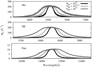
Figure 5.— Monte Carlo simulated profiles of Raman scattered radiation around H$\alpha$, H$\beta$ and Pa$\alpha$ (upper, middle and bottom panel, respectively) for various column densities $N_{HI}$ ranging from $10^{22}{\rm\ cm^{-2}}$ to $10^{23}{\rm\ cm^{-2}}$. As $N_{HI}$ increases, the wing profile broadens in roughly proportional to $N_{HI}^{1/2}$.

In Fig. 5, we investigate the Balmer and Paschen wings that are simulated for various values of $N_{\rm HI}$. In this figure, we set $R_{i}=10{\rm\ pc}$ and $H=R_{o}=20{\rm\ pc}$. We vary the number density of H I in such a way that the neutral column density $N_{\rm HI}$ in the lateral direction becomes $10^{22},\ 10^{22.5}$ and $10^{23}{\rm\ cm^{-2}}$.

Because the covering factor of the neutral scattering region is fixed and the total scattering optical depth is very large near line core, the Raman flux at line center remains the same for various values of $N_{\rm HI}$. The primary effect of varying $N_{\rm HI}$ is the width of the Raman wings, in that the width is roughly proportional to $N_{\rm HI}^{1/2}$. As $N_{\rm HI}$ increases, the saturated part also extends further away from the line center.

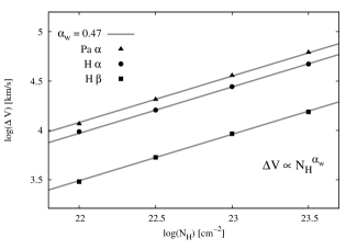
Figure 6.— Widths of Monte Carlo simulated Raman wings around H$\alpha$, H$\beta$ and Pa$\alpha$ considered in Fig. 5. The horizontal and vertical axes represent the column density and the wing width, respectively. Both axes are in logarithm scale. The dots are measured values from the Monte Carlo simulation and the fitting lines have a slope of 0.47.

We define the width of Raman wings as the difference of the two Doppler factors that correspond to the half values of the Raman flux at line center. Using this definition, we plot the Raman wing widths for various column densities in Fig. 6. Note that both the vertical and the horizontal scales are logarithmic. The Monte Carlo simulated data are shown by the dots that are fitted by lines having a slope of 0.47. In terms of the parameter $N_{23}=N_{\rm HI}/(10^{23}{\rm\ cm^{-2}})$ the fitting lines are explicitly written as

$$\Delta V_{\rm H\alpha} = 2.75\times 10^{4}\ N_{23}^{0.47}\ {\rm km\ s^{-1}}$$

$$\Delta V_{\rm H\beta} = 9.12\times 10^{3}\ N_{23}^{0.47}\ {\rm km\ s^{-1}}$$

$$\Delta V_{\rm Pa\alpha} = 3.55\times 10^{4}\ N_{23}^{0.47}\ {\rm km\ s^{-1}}.$$ (19)

In order to investigate the effect of the covering factor of the scattering region, we vary the height $H$ of the scattering region with the parameters $R_{i}=10{\rm\ pc}$, $R_{o}=20{\rm\ pc}$ and $N_{\rm HI}=10^{23}{\rm\ cm^{-2}}$ fixed. We show our result in Fig. 8 for values of $A=0.5,1,2$ and $\infty$.

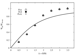
Figure 7.— Relative strengths of Monte Carlo simulated Raman wings around H$\alpha$, H$\beta$ and Pa$\alpha$ considered in Fig. 8. The vertical axis represents the wing strengths normalized with the Raman wing strength for $A=\infty$. The solid curve shows the covering factor $f(A)={A\over\sqrt{4+A^{2}}}$ of the scattering region, whose behavior is also characterized by linearity for small $A$ and approaching unity as $A\to\infty$.

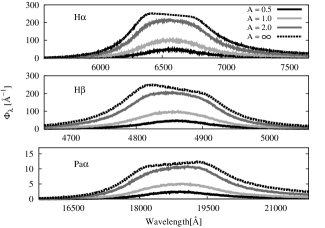
Figure 8.— Monte Carlo simulated profiles of Raman scattered radiation around H$\alpha$, H$\beta$ and Pa$\alpha$ (upper, middle and bottom panel, respectively) for various covering factors. $A=H/\Delta R$ is the ratio of the height and the thickness of the cylindrical shell.

With $A\leq 2$ the wing profiles are smooth. Even though not shown in the figure, we checked that there appears an inclined plateau around line center in each Raman wing for $A\geq 4$, implying the saturation behavior.

As the covering factor increases, more far UV photons are incident into the scattering region leading to stronger Raman scattering wings. When $A$ is small, the Raman wing strength is approximately linearly proportional to $A$. However if $A$ exceeds 2, the wing strength increases very slowly and approaches a limiting value. Given $A$ we normalize the H$\alpha$ Raman wing strengths by dividing the total number of Raman H$\alpha$ wing photons by that for $A=\infty$. The wing strengths for H$\beta$ and Pa$\alpha$ are normalized in a similar way. In Fig. 7, we plot the normalized wing strengths for H$\alpha$, H$\beta$ and Pa$\alpha$ by triangles, circles and squares, respectively. Given $A$ and $N_{HI}$, the normalized strengths are almost equal to each other for H$\alpha$, H$\beta$ and Pa$\alpha$ wings. For reference, we add the solid curve to show the covering factor of the scattering region given by

$$f(A)={A\over\sqrt{4+A^{2}}}.$$ (20)

The covering factor also shows a similar behavior of linearity for small $A$ and approaching unity for large $A$. Significant deviations between the normalized Raman wing strengths and the covering factor are attributed to complicated effects of multiple scattering and branching channels associated with the formation of Raman wings.

4.4. Mock Spectrum around Balmer Lines

In order to assess the observational feasibility we produce a mock spectrum around Balmer lines by superposing the wing profiles onto artificially produced H$\alpha$ and H$\beta$ broad emission lines. In Fig. 9, we show our result. In the production of the mock spectrum we assumed that the continuum level around Ly$\beta$ and Ly$\gamma$ is given by the fixed value of $\lambda L_{\lambda}=10^{44}{\rm\ erg\ s^{-1}}$ and that the continuum between H$\beta$ and H$\alpha$ is given in such a way that $L_{\lambda}=10^{40}{\rm\ erg\ s^{-1}\AA^{-1}}$. We also set the luminosity distance $D_{L}=0.3{\rm\ Gpc}$.

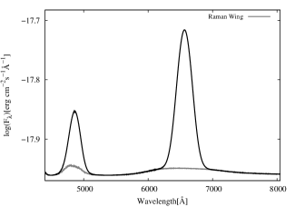
Figure 9.— Mock composite spectrum around H$\alpha$ and H$\beta$ with Raman scattering wings. The gray line shows Raman wings generated through a Monte Carlo simulation. The vertical scale is logarithmic for clear view of Raman wings against prominent emission lines.

With no established line profiles of the Balmer emission lines in AGNs, we take a Gaussian profile of width $5,000{\rm\ km\ s^{-1}}$ for H$\alpha$ and H$\beta$ emission lines. We set the equivalent widths of H$\alpha$ and H$\beta$ broad emission lines to be 200 Å and 50 Å, respectively. The scattering geometry is taken so that $R_{i}=10\>{\rm pc},R_{o}=20\>{\rm pc}$ and $H=20\>{\rm pc}$ with $N_{\rm HI}=5\times 10^{23}\>{\rm cm^{-2}}$.

In the figure the vertical scale is logarithmic and the Raman wings are shown by gray solid lines. In the case of H$\beta$, the Raman wings are inconspicuous because the broad emission component dominates the relatively narrow Raman H$\beta$ wings. However, the Raman H$\alpha$ wings are sufficiently wide to be observationally detectable. It is an interesting possibility that type 2 AGNs may also show detectable Raman H$\beta$ wings, which will be seen outside of the narrow H$\beta$ emission line.

5. Summary and Discussion

In this article we produced Raman wing profiles expected around H$\alpha$, H$\beta$ and Pa$\alpha$ that are formed by far UV continuum radiation scattered in a thick neutral region surrounding the central engine. The strengths of Raman wings are mainly determined by the product of the covering factor and the neutral column density of the scattering region. The wing width is approximately proportional to $N_{\rm HI}^{1/2}$. We also provide a mock spectrum by superposing simulated Raman wings onto artificially generated broad emission lines of H$\alpha$ and H$\beta$.

Observationally the Raman wings are difficult to discern from the underlying continuum because of their large width. Another issue may be that broad wings can also be formed from Thomson scattering or hot tenuous fast wind that emits Balmer and Paschen line photons (Kim et al. (2007)). One distinguishing aspect of the Raman wings is the differing widths and profiles exhibited by H$\alpha$, H$\beta$ and Pa$\alpha$ because of the complicated atomic physics. If the wings are formed in an emission region moving very fast, then all the wings are expected to show similar widths and profiles.

Another important characteristic is the linear polarization because the scattering mechanism is exactly the E-1 process, which also characterizes the Thomson scattering (Trippe (2014)). Ogle et al. (1997) performed spectropolarimetry of the prototypical narrow line radio galaxy Cyg A using the Keck II Telescope, in which they discovered extremely broad H$\alpha$ in the polarized flux. The full width at half-maximum of polarized H$\alpha$ is $26,000{\rm\ km\ s^{-1}}$. If this huge width is attributed to dust scattering or free electron scattering, one may need to assume that the velocity scale of the hidden broad line region is roughly the same value of $26,000{\rm\ km\ s^{-1}}$. In this case, the relativistic beaming inevitably leads to very asymmetric profiles with the blue part much stronger than the red part.

On the other hand, very broad features around H$\alpha$ are naturally formed through Raman scattering of far UV radiation without invoking extreme kinematics in the broad emission line region. For example, if we assume that the central engine of Cyg A is surrounded by a cold thick region with $N_{\rm HI}\sim 10^{23}{\rm\ cm^{-2}}$ the width of $26,000{\rm\ km\ s^{-1}}$ can be explained. In this case, we have to assume that the continuum around Ly$\gamma$ is relatively weak compared to that around Ly$\beta$ in order to explain no detection of the polarized broad features around H$\beta$. In particular, it is highly noticeable that Reynolds et al. (2015) proposed a neutral column density of $\sim 1.6\times 10^{23}{\rm\ cm^{-2}}$ from their observations of NUSTAR of Cyg A. Despite the difficulty in identifying the broad wings around H I emission lines from the local continuum, they will provide important clues to the unification model of AGNs.

References

- Antonucci (1993) Antonucci, R., 1993, ARAA, 31, 473
- Antonucci & Miller (1985) Antonucci, R. R. J., Miller, J. S., 1985, ApJ, 297, 621
- Bach & Lee (2014) Bach, K. & Lee, H.-W., 2014, JKAS, 47, 187
- Bethe & Salpeter (1957) Bethe, H. A. & Salpeter, E. E., 1957, Quantum Mechanics of One- and Two-Electron Atoms, New York, Academic Press
- Bentz et al. (2009) Bentz, M. C. et al., 2009, ApJ, 705, 199
- Blandford & McKee (1982) Blandford, R. D., McKee, C. F., 1982, ApJ, 255, 419
- Chiang et al. (2013) Chiang, C.-Y., Cackett, E. M., Gandhi, P., & Fabian, A., 2013, MNRAS, 430, 2943
- Cohen et al. (1995) Cohen, M. H., Ogle, P. M., Tran, H. D., Vermeulen, R. C., Miller, J. S., Goodrich, R. W., Martel, A. R., 1995, ApJ, 448, L77
- Dietrich et al. (2012) Dietrich, M. et al., 2012, ApJ, 757, 53
- Kenyon (1986) Kenyon, S. J., 1986, The Symbiotic Stars, Cambridge : Cambridge University Press
- Kim et al. (2007) Kim, H. J., Lee, H.-W. & Kang, S., 2007, MNRAS, 374, 187
- Lee & Blandford (1997) Lee, H.-W., & Blandford, R. D., 1997, MNRAS, 288, 19
- Lee & Yun (1998) Lee, H.-W., & Yun, J. H., 1998, MNRAS, 301, 193
- Lee (2000) Lee, H.-W., 2000, ApJ, 541, L25
- Lee (2013) Lee, H.-W., 2013, ApJ, 772, 123
- Murray & Chiang (1995) Murray, N., Chiang, J., 1995, ApJ, 454, 105
- Nussbaumer et al. (1989) Nussbaumer, H., Schmid, H. M., Vogel, M., 1989, A&A, 211, L27
- Ogle et al. (1997) Ogle, P. M., Cohen, M. H., Miller, J. S., Tran, H. D., Fosbury, R. A. E., Goodrich, R. W., 1997, ApJ, 482, L37
- Park et al. (2012) Park, Daeseong, 2012, ApJ, 747, 30
- Peterson (1993) Peterson, B. M., 1993, PASP, 105, 247
- Peterson (1997) Peterson, B. M. 1997, An Introduction to Active Galactic Nuclei, Cambridge: Cambridge University Press
- Reynolds et al. (2015) Reynolds, C. S., et al., 2015, ApJ
- Sakurai (1967) Sakurai, J. J., 1967, Advanced Quantum Mechanics, Reading: Addison-Wesley
- Saslow & Mills (1969) Saslow, W. M., Mills, D. L., 1969, Physical Review, 187, 1025
- Schmid (1989) Schmid, H. M., 1989, A&A, 211, L31
- Trippe (2014) Trippe, S., 2014, JKAS, 47, 15
- Vanden Berk et al. (2001) Vanden Berk, D. E., et al., 2001, AJ, 122, 549
- Yoo et al. (2002) Yoo, J. J., Bak, J.-Y., Lee, H.-W., 2002, MNRAS, 336, 467
- Zheng al. (1997) Zheng Wei, Kriss, Gerard A., Telfer, Randal C., Grimes, John P., Davidsen, Arthur F., 1997, AJ, 475, 469