Sintering-induced Dust Ring Formation in Protoplanetary Disks: Application to the HL Tau Disk

Abstract

The latest observation of HL Tau by ALMA revealed spectacular concentric dust rings in its circumstellar disk. We attempt to explain the multiple ring structure as a consequence of aggregate sintering. Sintering is known to reduce the sticking efficiency of dust aggregates and occurs at temperatures slightly below the sublimation point of their constituent material. We here present a dust growth model incorporating sintering and use it to simulate global dust evolution due to sintering, coagulation, fragmentation, and radial inward drift in a modeled HL Tau disk. We show that aggregates consisting of multiple species of volatile ices experience sintering, collisionally disrupt, and pile up at multiple locations slightly outside the snow lines of the volatiles. At wavelengths of 0.87–1.3 mm, these sintering zones appear as bright, optically thick rings with a spectral slope of $\approx 2$, whereas the non-sintering zones as darker, optically thinner rings of a spectral slope of $\approx 2.3$–$2.5$. The observational features of the sintering and non-sintering zones are consistent with those of the major bright and dark rings found in the HL Tau disk, respectively. Radial pileup and vertical settling occur simultaneously if disk turbulence is weak and if monomers constituting the aggregates are $\sim 1~{}\micron$ in radius. For the radial gas temperature profile of $T=310(r/1~{}{\rm AU})^{-0.57}~{}{\rm K}$, our model perfectly reproduces the brightness temperatures of the optically thick bright rings, and reproduces their orbital distances to an accuracy of $\lesssim 30\%$.

1. Introduction

HL Tau is a flat spectrum T Tauri star with a circumstellar disk that is very luminous at millimeter wavelengths (Beckwith et al., 1990). Although the age of HL Tau has not been well constrained, its low bolometric temperature, high mass accretion rate (e.g., White & Hillenbrand, 2004) and the presence of an optical jet (Mundt et al., 1988) and an infalling envelope (Hayashi et al., 1993) suggest that the stellar age is likely less than 1 Myr. For these reasons, HL Tau is considered as an ideal observational target for studying the very initial stages of disk evolution and of planet formation.

The recent Long Baseline Campaign of the Atacama Large Millimeter/submillimeter Array (ALMA) has provided spectacular images of the HL Tau disk (ALMA Partnership et al., 2015). ALMA resolved the disk at three millimeter wavelengths with unprecedented spatial resolution of $\approx 3.5$ AU at 0.87 mm. The observations revealed a pattern of multiple bright and dark rings that are remarkably symmetric with respect to the central star. The spectral index at 1 mm is $\sim 2$ in the central emission peak and in some of the bright rings, and is $\sim 2.3$–$3$ in the dark rings (ALMA Partnership et al., 2015; Zhang et al., 2015). The fact that the millimeter spectral index is $\lesssim 3$ in the dark, presumably optically thin rings suggests that dust grains in the HL Tau disk have already grown into aggregates whose radius is larger than a few millimeters, assuming that the aggregates are compact (Draine, 2006, see Kataoka et al. 2014 for how the aggregates’ porosity alters this interpretation). The observed continuum emission is best reproduced by models assuming substantial dust settling (Kwon et al., 2011, 2015; Pinte et al., 2016), implying that the large aggregates are dominant in mass and that the turbulence in the gas disk is weak. Since dust growth and settling are key processes in planet formation, understanding the origin of this axisymmetric dust structure is greatly relevant to understanding how planets form in protoplanetary disks.

There are a variety of mechanisms that can produce axisymmetric dust rings and gaps in a protoplanetary disk. One of the most common mechanisms creating a dust ring is dust trapping at local gas pressure maxima under the action of gas drag (Whipple, 1972). In a protoplanetary disk, pressure bumps may be created by disk–planet interaction (Paardekooper & Mellema, 2004, 2006; Fouchet et al., 2010; Zhu et al., 2012; Pinilla et al., 2012; Gonzalez et al., 2012; Dong et al., 2015; Dipierro et al., 2015), magnetorotational instability (Johansen et al., 2009; Uribe et al., 2011), and/or steep radial variation of the disk viscosity (Kretke & Lin, 2007; Dzyurkevich et al., 2010; Flock et al., 2015). Axisymmetric dust rings may also be produced by secular gravitational instability (Youdin, 2011; Takahashi & Inutsuka, 2014), by baroclinic instability arising due to dust settling (Lorén-Aguilar & Bate, 2015), or by a combined effect of dust coagulation and radial drift (Laibe, 2014; Gonzalez et al., 2015). Planet-carved gaps may explain the observed features of the HL Tau disk even if dust trapping at the pressure maxima is ineffective (Kanagawa et al., 2015).

Another intriguing possibility is that the multiple ring patterns of the HL Tau disk are related to the snow lines of various solid materials. Recently, Zhang et al. (2015) used a temperature profile based on a previous study (Men’shchikov et al., 1999) and showed that the major dark rings seen in the ALMA images lie close to the sublimation fronts of some main cometary volatiles such as ${\rm H_{2}O}$ and ${\rm NH_{3}}$. They interpreted this as the evidence of rapid particle growth by condensation as recently predicted by Ros & Johansen (2013) for ${\rm H_{2}O}$ ice particles. However, it is unclear at present whether relatively minor volatiles such as ${\rm NH_{3}}$ and clathrates indeed accelerate dust growth.

In this study, we focus on another important mechanism that can affect dust growth near volatile snow lines: sintering. Sintering is the process of fusing grains together at a temperature slightly below the sublimation point. Sintered aggregates are characterized by thick joints, called necks, that connect the constituent grains (e.g., see Figures 3 and 4 of Poppe 2003; Figure 1 of Blackford 2007). A familiar example of a sintered aggregate is a ceramic material (i.e., pottery), which is an agglomerate of micron-sized clay particles fused together by sintering. Sintered aggregates are less sticky than unsintered ones, because the necks prevent collision energy from being dissipated through plastic deformation. For example, unsintered dust aggregates are known to absorb much collision energy through rolling friction among constituent grains (Dominik & Tielens, 1997). However, sintered aggregates are unable to lose their collision energy in this way, and therefore their collision tends to end up with bouncing, fragmentation, or erosion rather than sticking (Sirono, 1999; Sirono & Ueno, 2014). Thus, sintering suppresses dust growth in regions slightly outside the snow lines.

The importance of sintering in the context of protoplanetary dust growth was first pointed out by Sirono (1999), and has been studied in more detail by Sirono (2011a, b) and Sirono & Ueno (2014). Sirono (1999) simulated collisions of two-dimensional sintered and unsintered aggregates (both made of $0.1~{}\micron$-sized icy grains) with a wall taking into account the high mechanical strength of the sintered necks. At collision velocities lower than $10~{}{\rm m~{}s^{-1}}$, the sintered aggregates are found to bounce off the wall whereas the unsintered ones stick to the wall. By using the same sintered neck model, Sirono & Ueno (2014) simulated collisions between two identical sintered aggregates each of which consists of up to $10^{4}$ icy grains (again of $0.1~{}\micron$ radius) and has a porosity of 30–80%. They found that the aggregates erode each other rather than stick if the collision velocity is above $20~{}{\rm m~{}s^{-1}}$. This threshold is considerably lower than that for unsintered aggregates, which is around $50~{}{\rm m~{}s^{-1}}$ when the constituent grains are ice and $0.1~{}\micron$ in radius (Dominik & Tielens, 1997; Wada et al., 2009, 2013).

Another important fact about sintering is that it can occur at multiple locations in a protoplanetary disk as already pointed out by Sirono (1999, 2011b). In contrast to condensational growth as envisioned by Zhang et al. (2015), sintering requires only a small amount of volatiles because the volume of a neck is generally a small fraction of the grain volume. For example, the volume fraction is only $0.2\%$ even if the neck radius is as large as $30\%$ of the grain radius (Sirono, 2011b). Therefore, inclusion of ${\rm NH_{3}}$ ice at a standard cometary abundance ($\sim 0.2$–$1.4\%$; Mumma & Charnley 2011) is enough to sinter the grains near the ${\rm NH_{3}}$ snow line.

In this study, we investigate how this “sintering barrier” against dust coagulation affects the global evolution of dust in a protoplanetary disk. We present a simple recipe to account for the change in the mechanical strength of dust aggregates due to sintering, and apply it to global simulations of dust evolution in a disk that take into account coagulation, fragmentation, and radial inward drift induced by gas drag (Adachi et al., 1976; Weidenschilling, 1977). Our simulations for the first time show that sintering-induced fragmentation leads to a pileup of dust materials in the vicinity of each volatile snow line. We will demonstrate that at millimeter wavelengths, these pileups can be seen as multiple bright dust rings as observed in the HL Tau disk.

The structure of this paper is as follows. We begin by modeling the HL Tau gas disk in Section 2. Section 3 introduces our model for aggregate sintering and sublimation. Section 4 describes our simulation method, Section 5 presents the results from our fiducial simulation run, and Section 6 presents a parameter study. The validity and possible limitations of our model are discussed in Section 7. A summary is presented in Section 8.

2. Disk Model

We model the HL Tau protoplanetary disk as a static, axisymmetric, and vertically isothermal disk. The radial profiles of the temperature and gas density are presented in Sections 2.1 and 2.2, respectively.

2.1. Temperature Profile

We construct a radial temperature profile $T(r)$ of the HL Tau disk based on the data of the surface brightness profiles provided by ALMA Partnership et al. (2015). We deproject the intensity maps of the disk’s dust continuum at ALMA Bands 3, 6, and 7 into circularly symmetric views assuming the disk inclination angle of $46.7^{\circ}$ and the position angle of $138^{\circ}$ (ALMA Partnership et al., 2015). We then obtain the radial profiles of the intensities $I_{\nu}$ by azimuthally averaging the deprojected images. The upper panel of Figure 1 shows the derived radial emission profiles. Here, the intensities are expressed in terms of the Planck brightness temperature $T_{\rm B}$. Shown in the lower panel is the spectral index between Bands 6 and 7, $\alpha_{\rm B6\textrm{--}B7}\equiv\ln(I_{\rm B7}/I_{\rm B6})/\ln(\nu_{\rm B7}/\nu_{\rm B6})$, where $\nu_{\rm B6}=233.0~{}{\rm GHz}$ and $\nu_{\rm B7}=343.5~{}{\rm GHz}$ are the frequencies at Bands 6 and 7, respectively.

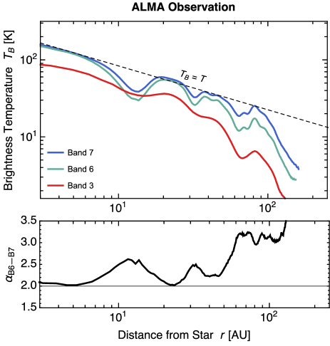
Figure 1.— Upper panel: radial profiles of the brightness temperature $T_{B}$ of the HL Tau disk retrieved from the ALMA data (ALMA Partnership et al. 2015; see text for details). The red, green, and blue curve are for ALMA Bands 3, 6, and 7, respectively. The dashed line shows the gas temperature profile $T(r)$ adopted in this study (Equation (1)). Lower panel: spectral index between Bands 6 and 7, $\alpha_{\rm B6\textrm{--}B7}$, versus radial distance $r$.

As already pointed out by ALMA Partnership et al. (2015), the HL Tau disk has a pronounced central emission peak at $\lesssim 10$ AU, and three major bright rings at $\sim 20$, 40, and 80 AU. The central emission peak and two innermost bright rings have a spectral index of $\alpha_{\rm B6\textrm{--}B7}\approx 2$. In general, this indicates either that the emission at these wavelengths is optically thick, or that the emission is optically thin but is from dust particles larger than millimeters. The brightness temperature is equal to the gas temperature in the former case, and is lower in the latter case. While Zhang et al. (2015) adopted the latter interpretation, we here pursue the former interpretation. Specifically, we assume that the Band 7 emission is optically thick and hence $T(r)=T_{\rm B}$ at the center, 20 AU, and 40 AU. The simplest profile satisfying this assumption is the single power law

$$T(r)=310\biggl{(}{\displaystyle\frac{r}{1~{}{\rm AU}}}\biggr{)}^{-0.57}~{}{\rm K},$$ (1)

which is shown by the dashed line in the upper panel of Figure 1. We will adopt this temperature profile in this study.

2.2. Density Structure

The density structure of the HL Tauri gas disk is unknown. Therefore, we simply assume that the gas surface density $\Sigma_{\rm d}(r)$ obeys a power law with an exponential taper (Hartmann et al., 1998; Kitamura et al., 2002; Andrews et al., 2009),

$$\Sigma_{\rm g}(r)=\frac{(2-\gamma)M_{\rm disk}}{2\pi r_{c}^{2}}\biggl{(}{\displaystyle\frac{r}{r_{\rm c}}}\biggr{)}^{-\gamma}\exp\left[-\biggl{(}{\displaystyle\frac{r}{r_{c}}}\biggr{)}^{2-\gamma}\right],$$ (2)

where $r_{\rm c}$ and $M_{\rm disk}$ are a characteristic radius and the total mass of the gas disk, respectively, and $\gamma$ ($0<\gamma<2$) is the negative slope of $\Sigma_{\rm g}$ at $r\ll r_{\rm c}$. We take $\gamma=1$ as the fiducial value but also consider $\gamma=0.5$ and 1.5. The dependence of our simulation results on $\gamma$ will be studied in Section 6.1. The values of $M_{\rm disk}$ and $r_{\rm c}$ are fixed to $0.2M_{\sun}$ and $150~{}{\rm AU}$, respectively. The adopted disk mass is about twice the upper end of the previous mass estimates for the HL Tau disk (Guilloteau et al., 2011; Kwon et al., 2011, 2015). We assume such a massive disk because the dust mass in the disk decreases with time due to the radial drift of dust particles (see Section 5.1). Figure 2 shows the surface density profiles for $\gamma=1$, 0.5, and 1.5.

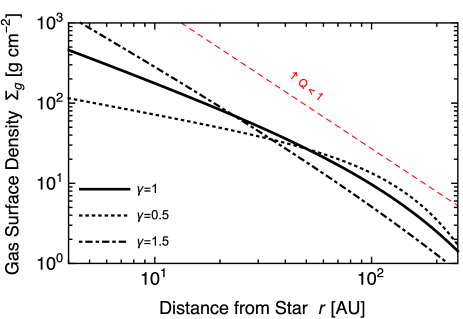
Figure 2.— Radial profiles of the gas surface density $\Sigma_{\rm g}$ adopted in this study (Equation (2)). The solid, dotted, and dot-dashed lines are for $\gamma=1$ (fiducial), 0.5, and 1.5, respectively. The dashed line shows $Q\equiv c_{s}\Omega/\pi G\Sigma_{\rm g}=1$.

Since the disk is assumed to be vertically isothermal, the vertical distribution of the gas density obeys a Gaussian with the midplane value $\rho_{\rm g}=\Sigma_{\rm g}/(\sqrt{2\pi}H_{\rm g})$, where $H_{\rm g}=c_{s}/\Omega$ is the gas scale height, $c_{\rm s}$ is the sound speed, and $\Omega$ is the Keplerian frequency. The isothermal sound speed is given by $c_{\rm s}=\sqrt{k_{\rm B}T/m_{\mu}}$, where $k_{\rm B}$ is the Boltzmann constant and $m_{\mu}$ is the mean molecular mass of the disk gas assumed to be $m_{\mu}=2.3~{}{\rm amu}$. The Keplerian frequency is given by $\Omega=\sqrt{GM_{*}/r^{3}}$, where $G$ is the gravitational constant and $M_{*}$ is the stellar mass. We adopt $M_{*}=1M_{\odot}$ so that the sum of the stellar and disk masses in the fiducial model, $M_{*}+M_{\rm disk}=1.2M_{\sun}$, is within the range of the previous estimates for the HL Tau system (Beckwith et al., 1990; Sargent & Beckwith, 1991; ALMA Partnership et al., 2015).

We note here that the assumed disk model is marginally gravitationally stable: the Toomre stability parameter $Q\equiv c_{\rm s}\Omega/(\pi G\Sigma_{\rm g})$ satisfies $Q\gtrsim 1$ at all radii for all choices of $\gamma$. This can be seen in Figure 2, where the surface density corresponding to $Q=1$ is shown by the dashed line.

3. Sublimation and Sintering of Icy Dust

We model dust in the HL Tau disk as aggregates of (sub)micron-sized grains. Each constituent grain, which we call a monomer, is assumed to be coated by an ice mantle composed of various volatile molecules (Section 3.1). The composition of the mantle at a given distance from the central star is determined by using the equilibrium vapor pressure curves for the volatile species (Sections 3.2 and 3.3). The equilibrium vapor pressures also determine the rate at which the sintering of aggregates proceeds at each orbital distance (Section 3.4). The sintering rate will be used to determine the sticking efficiency of the aggregates in our dust coagulation simulations (see Section 4.4).

3.1. Volatile Composition

Table 1Abundances of Major Cometary Volatiles Relative to ${\rm H_{2}O}$ (in Percent)

Species	Cometary Value	Adopted Value $f_{j}$
${\rm H_{2}O}$	100	100
${\rm NH_{3}}$	0.2–1.4	1
${\rm CO_{2}}$	2–30	10
${\rm H_{2}S}$	0.12–1.4	1
${\rm C_{2}H_{6}}$	0.1–2	1
${\rm CH_{4}}$	0.4–1.6	1
CO	0.4–30	10

We assume that the volatile composition of the HL Tau disk is similar to that of comets in our solar system. We select six major cometary volatiles in addition to ${\rm H_{2}O}$ and take their abundances relative to ${\rm H_{2}O}$ to be consistent with cometary values (Mumma & Charnley, 2011). The volatiles we select are ammonia (${\rm NH_{3}}$), carbon dioxide (${\rm CO_{2}}$), hydrogen sulfide (${\rm H_{2}S}$), ethane (${\rm C_{2}H_{6}}$), methane (${\rm CH_{4}}$), and carbon monoxide (CO). We neglect another equally abundant species, methanol (${\rm CH_{3}OH}$), because the snow line of ${\rm CH_{3}OH}$ is very close to that of more abundant ${\rm H_{2}O}$ (Sirono, 2011b). Table 1 lists the abundances we adopt and the observed ranges of cometary abundances taken from Mumma & Charnley (2011).

3.2. Equilibrium Vapor Pressures

Table 2Vapor Pressure Parameters

Species	$L_{j}$ (K)	$A_{j}$	Ref.	$L_{j,\rm tuned}$ (K)
${\rm H_{2}O}$	6070	30.86	1	5463
${\rm NH_{3}}$	3754	30.21	2	3379
${\rm CO_{2}}$	3148	30.01	2	$\cdots$
${\rm H_{2}S}$	2860	27.70	3	$\cdots$
${\rm C_{2}H_{6}}$	2498	30.24	4	2248
${\rm CH_{4}}$	1190	24.81	2	$\cdots$
CO	981.8	26.41	2	$\cdots$

References. — (1) Bauer et al. (1997), (2) Yamamoto et al. (1983), (3) Haynes (2014), (4) Moses et al. (1992).

The equilibrium vapor pressures of volatiles determine the temperatures at which sublimation and sintering occurs. In this study, we approximate the equilibrium vapor pressure for each volatile species $j$ by the Arrhenius form

$$P_{{\rm ev},j}=\exp\left(-\frac{L_{j}}{T}+A_{j}\right)~{}{\rm dyn~{}cm^{-2}},$$ (3)

where $L_{j}$ is the heat of sublimation in Kelvin and $A_{j}$ is a dimensionless constant. Table 3.2 summarizes the values of $L_{j}$ and $A_{j}$ for the seven volatile species considered in this study. For ${\rm CO}$, ${\rm CH_{4}}$, ${\rm CO_{2}}$, and ${\rm NH_{3}}$, we follow Sirono (2011b) and take the values from Table 2 of Yamamoto et al. (1983). The values for ${\rm C_{2}H_{6}}$ are derived from the analytic expression of the vapor pressure by Moses et al. (1992, see their Table III; note that we here neglect the small offset in $T$ in their original expression). For ${\rm H_{2}S}$, we determined $L_{j}$ and $A_{j}$ by fitting Equation (3) to the vapor pressure data provided by Haynes (2014, page 6-92). Figure 3 shows $P_{{\rm ev},j}$ of the seven volatile species as a function of $r$ for the temperature distribution given by Equation (1).

Strictly speaking, the vapor pressure data given in Table 3.2 only apply to pure ices. In protoplanetary disks, volatiles may be trapped inside the ${\rm H_{2}O}$ mantle of dust grains instead of being present as pure ices. If this is the case, the volatiles would sublimate not only at the sublimation temperatures for pure ices but also at higher temperatures where monolayer desorption from the ${\rm H_{2}O}$ substrate, phase transition of ${\rm H_{2}O}$ ice, or co-desorption with the ${\rm H_{2}O}$ ice takes place (Collings et al., 2003, 2004; Martín-Doménech et al., 2014). However, all these high-temperature desorption processes are irrelevant to neck formation (sintering) because the desorbed molecules are unable to recondense onto grain surfaces at such high temperatures. By using the vapor pressure data for pure ices, we effectively neglect all these desorption processes.

When estimating the locations of the snow lines, it is important to note that the vapor pressure data in the literature are subject to small but still non-negligible uncertainties. For example, the values of the sublimation energies we use for ${\rm H_{2}O}$, ${\rm NH_{3}}$, ${\rm CO_{2}}$, and ${\rm CO}$ are 10–20% higher than those derived from the very recent temperature programmed desorption experiments by Martín-Doménech et al. (2014, see their Table 4). Luna et al. (2014) compiled the sublimation energies of major cometary volatiles from different experimental methods, and showed that the published sublimation energies have standard deviation of 14, 8, 11, and 8% for ${\rm NH_{3}}$, ${\rm CO_{2}}$, ${\rm CH_{4}}$ and ${\rm CO}$, respectively (see their Table 2 and Figures 4 and 5). Such uncertainties might be present in the vapor pressure data for other volatiles species. As we will demonstrate in Section 6.4, even a 10% uncertainty in $L_{j}$ can lead to a 20–30% uncertainty in the location of its snow line, and a better match between our simulation results and the ALMA observation can be achieved if the sublimation energies of ${\rm H_{2}O}$, ${\rm NH_{3}}$, and ${\rm C_{2}H_{6}}$ are taken to be 10% lower than the fiducial values. We will denote these tuned sublimation energies by $L_{j,\rm tuned}$ (see Table 3.2). For ${\rm H_{2}O}$ and ${\rm NH_{3}}$, the tuned sublimation energies are more consistent with the results of Martín-Doménech et al. (2014).

3.3. Snow Lines

For each volatile species $j$, we define the snow line as the orbit inside which the equilibrium pressure $P_{{\rm ev},j}$ exceeds the partial pressure $P_{j}$. Assuming that the disk gas is well mixed in the vertical direction, $P_{j}$ is related to the surface number density of $j$-molecules in the gas phase, $N_{j}$, as

$$P_{j}=\frac{N_{j}k_{\rm B}T}{\sqrt{2\pi}H_{\rm g}}.$$ (4)

In this study, we do not directly treat the evolution of $N_{j}$ but instead estimate them by assuming that the ratio between $N_{j}$ and the surface number density of ${\rm H_{2}O}$ molecules in the solid phase is equal to the cometary abundance $f_{j}$ given in Table 1. We also assume that the mass fraction of ${\rm H_{2}O}$ ice inside the aggregates is 50%. Under these assumptions, $N_{j}$ can be expressed as

$$N_{j}=\frac{0.5f_{j}\Sigma_{\rm d}}{m_{\rm mol,H_{2}O}}.$$ (5)

The adopted relative abundances give the relations $P_{j}=0.1P_{\rm H_{2}O}$ for $j={\rm CO}$ and ${\rm CO}_{2}$, and $P_{j}=0.01P_{\rm H_{2}O}$ for $j={\rm NH_{3}}$, ${\rm H_{2}S}$, ${\rm C_{2}H_{6}}$, and ${\rm CH_{4}}$. For the purpose of calculating the locations of the snow lines, the simplification made here is acceptable as a first-order approximation, because the locations of the snow lines are predominantly determined by the strong dependence of $P_{{\rm ev},j}$ on $T(r)$ and are much less sensitive to a change in $P_{j}$.

To see the approximate locations of the snow lines in our HL Tau disk model, we shall now temporarily assume the standard dust-to-gas mass ratio of $\Sigma_{\rm d}=0.01\Sigma_{\rm g}$ throughout the disk. The dashed, dot-dashed, and dotted lines in Figure 3 show the partial pressure curves $P_{j}=\{1,0.1,0.01\}P_{\rm H_{2}O}$ for the fiducial disk model ($\gamma=1$). For each volatile species, the location of the snow line is given by the intersection of $P_{{\rm ev},j}$ and $P_{j}$, which is indicated by a filled circle in Figure 3. In this example, the ${\rm H_{2}O}$ snow line lies at a radial distance of 3.5 AU, which is well interior to the innermost dark ring of the HL Tau disk lying at $\sim$ 13 AU (see Figure 1). Zhang et al. (2015) suggested that the ${\rm H_{2}O}$ snow line lies on the 13 AU dark ring assuming a higher gas temperature than ours. The snow lines of ${\rm NH_{3}}$, ${\rm CO_{2}}$, ${\rm H_{2}S}$, and ${\rm C_{2}H_{6}}$ are narrowly distributed over the intermediate region of 10–30 AU, and those of ${\rm CH_{4}}$ and ${\rm CO}$ are located in the outermost region of 100–150 AU.

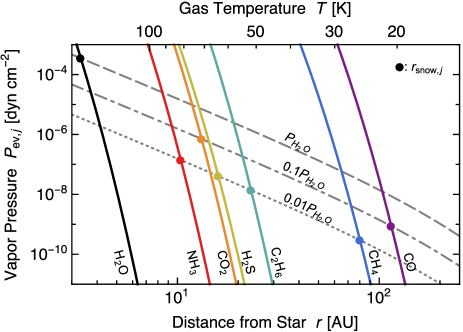
Figure 3.— Equilibrium vapor pressures $P_{{\rm ev},j}$ (Equation (3)) of major cometary volatiles as a function of orbital distance $r$ for the temperature profile given by Equation (1). From left to right: ${\rm H_{2}O}$ (black), ${\rm NH_{3}}$ (red), ${\rm CO_{2}}$ (orange), ${\rm H_{2}S}$ (yellow), ${\rm C_{2}H_{6}}$ (green), ${\rm CH_{4}}$ (blue), and CO (purple). The gray curves show the partial pressures of the volatiles (dashed curve for ${\rm H_{2}O}$, dot-dashed curve for ${\rm CO}$ and ${\rm CO_{2}}$, dotted curve for the other species) for the gas density profile given by Equation (2) with $\gamma=1$ and $\Sigma_{\rm d}=0.01\Sigma_{\rm g}$. The filled circles indicate the locations of the snow lines, $r=r_{{\rm snow},j}$.

3.4. Sintering Zones

Sintering is the process of neck growth, and its timescale is inversely proportional to the rate at which the neck radius increases (e.g., Swinkels & Ashby, 1981). The timescale depends on the size of monomers, with larger monomers generally leading to slower sintering. In this study, we simply assume monodisperse monomers and treat their radius $a_{0}$ as a free parameter (see Section 6.3 for parameter study). We only consider $a_{0}\leqslant 4~{}\micron$ because sintering is too slow to affect dust evolution in a protoplanetary disk beyond this size range (see below).

When neck growth is driven by vapor transport of volatile $j$, its timescale is given by (Sirono, 2011b)

$$t_{{\rm sint},j}=4.7\times 10^{-3}\frac{a_{0}^{2}(2\pi m_{{\rm mol},j})^{1/2}(k_{\rm B}T)^{3/2}}{P_{{\rm ev},j}(T)V_{{\rm mol},j}^{2}\gamma_{j}},$$ (6)

where $m_{{\rm mol},j}$, $V_{{\rm mol},j}$ and $\gamma_{j}$ are the molecular mass, molecular volume, and surface energy of the species, respectively. The small prefactor $4.7\times 10^{-3}$ comes from the fact that the neck radius is much smaller than $a_{0}$. In general, $t_{{\rm sint},j}$ rapidly decreases with increasing $T$ because $P_{{\rm ev},j}$ strongly depends on $T$. For species other than ${\rm H_{2}S}$ and ${\rm C_{2}H_{6}}$, we use the same set of $V_{{\rm mol},j}$ and $\gamma_{j}$ adopted by Sirono (2011b). The molecular volumes of ${\rm H_{2}S}$ and ${\rm C_{2}H_{6}}$ are estimated as $V_{\rm mol,H_{2}S}=5.7\times 10^{-23}~{}{\rm cm^{3}}$ and $V_{\rm mol,C_{2}H_{6}}=7.1\times 10^{-23}~{}{\rm cm^{3}}$ assuming that the densities of ${\rm H_{2}S}$ and ${\rm C_{2}H_{6}}$ solids are $1~{}{\rm g~{}cm^{-3}}$ and $0.7~{}{\rm g~{}cm^{-3}}$ (Moses et al., 1992), respectively. We assume that the surface energy of ${\rm H_{2}S}$ ice is equal to that of ${\rm H_{2}S}$ liquid, $30~{}{\rm erg~{}cm^{-2}}$ (Meyer, 1977). For ${\rm C_{2}H_{6}}$, we use $\gamma_{\rm C_{2}H_{6}}=40~{}{\rm erg~{}cm^{-2}}$, which is the value at $\sim 50~{}{\rm K}$ (Moses et al., 1992). The locations of the sintering lines discusses below are insensitive to the values of $V_{{\rm mol},j}$ and $\gamma_{j}$ because of the strong temperature dependence of $P_{{\rm ev},j}$.

The necks do not only grow but also are destroyed by at least two processes.

1. The necks evaporate when the ambient gas temperature exceeds the sublimation temperature of volatile $j$ hat constitutes the necks. This occurs at $r<r_{{\rm snow},j}$, where $r_{{\rm snow},j}$ is the orbital radius of the snow line of the volatile.

2. The necks break when the aggregate is plastically deformed by another aggregate upon collision. Unsintered aggregates are known to experience substantial plastic deformation even if the collision velocity is much below the fragmentation threshold (Dominik & Tielens, 1997; Wada et al., 2008). Therefore, fully sintered aggregates form only if they never collide with each other until the sintering is completed, i.e., only if the sintering timescale is shorter than their collision timescale, which we will denote by $t_{\rm coll}$. Since $t_{{\rm sint},j}$ falls off rapidly toward the central star, there exists a location $r=r_{{\rm sint},j}$ inside which $t_{{\rm sint},j}<t_{\rm coll}$ for a given volatile species $j$. In this study, we call such locations the sintering lines.

Taken together, each volatile species $j$ causes aggregate sintering only inside the annulus defined by $r_{{\rm snow},j}<r<r_{{\rm sint},j}$. We call such regions the sintering zones. Our sintering zones are essentially equivalent to the “sintering regions” of Sirono (2011b).

In order to know the locations of sintering zones, one needs to estimate $t_{\rm coll}$. In principle, the collision time can be calculated from the size, number density, and relative speed of aggregates as we will do in our simulations (see Equation (12)). In this subsection, we shall avoid such detailed calculations and instead use a useful formula $t_{\rm coll}=100\Omega^{-1}$, which is an approximate expression for the collision timescale of macroscopic aggregates in a turbulent disk with the dust-to-gas mass ratio of 0.01 (Takeuchi & Lin, 2005; Brauer et al., 2008). This is a rough estimate (see Sato et al., 2016), but still provides a reasonable estimate for $r_{{\rm sint},j}$ because $t_{{\rm sint},j}$ is a steep function of $r$.

In Figure 4, we plot the sintering timescales of the seven volatile species as a function of $r$ for our HL Tau disk model with $\gamma=1$. We also indicate $t_{\rm coll}=100\Omega^{-1}$ by the dotted lines, the location of the sintering lines ($r_{{\rm sint},j}$) by the open circles, and the locations of the sintering zones ($r_{{\rm snow},j}<r<r_{{\rm sint},j}$) by the horizontal bars. We here consider two different values of $a_{0}$, $0.1~{}\micron$ and $4~{}\micron$ (panels a and b, respectively), to highlight the importance of this parameter in our sintering model. For $a_{0}=0.1~{}\micron$, the width of each sintering zone is $30$–$50\%$ of $r_{{\rm sint},j}$, and the sintering zones of ${\rm NH_{3}}$, ${\rm CO_{2}}$, and ${\rm H_{2}S}$ significantly overlap with each other. A larger $a_{0}$ leads to longer sintering timescales and hence to narrower sintering zones. For $a_{0}=4~{}\micron$, the sintering zones for species other than ${\rm H_{2}O}$ almost disappear. For this reason, we will restrict ourselves to $a_{0}\leqslant 4~{}\micron$ in the following sections.

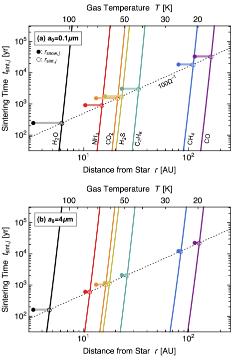
Figure 4.— Sintering timescales $t_{\rm sint}$ (Equation (6)) for major cometary volatiles as a function of orbital distance $r$ for our HL Tau disk model. From left to right: ${\rm H_{2}O}$ (black), ${\rm NH_{3}}$ (red), ${\rm CO_{2}}$ (orange), ${\rm H_{2}S}$ (yellow), ${\rm C_{2}H_{6}}$ (green), ${\rm CH_{4}}$ (blue), and CO (purple). Panels (a) and (b) are for monomer sizes $a_{0}=0.1~{}\micron$ and $4~{}\micron$, respectively. The dashed gray curve indicates $100\Omega^{-1}$, the typical timescale for particle collision in a disk (Takeuchi & Lin, 2005; Brauer et al., 2008). The filled circles indicate the locations of the snow lines, $r=r_{{\rm snow},j}$ (see also Figure 3), while the open circles indicate the locations of the sintering lines, $r=r_{{\rm sint},j}$. Icy aggregates experience sintering in the sintering zones defined by $r_{{\rm snow},j}<r<r_{{\rm sint},j}$ (horizontal bars).

4. Simulation Method

As introduced in Section 1, sintering is expected to reduce the sticking efficiency of dust aggregates. In protoplanetary disks, this can occur in the sintering zones defined in Section 3.4. To study how the presence of the sintering zones affects the radial distribution of dust in a disk, we conduct global simulations of dust evolution including sintering-induced fragmentation. In our simulations, we calculate the evolution of the surface density and representative size of icy aggregates due to coagulation and radial drift using the single-size approach (Section 4.1). The radial drift is due to the aerodynamical drag by the gas disk (Adachi et al., 1976; Weidenschilling, 1977), and its velocity depends on the size of the aggregates and on the gas surface density (Section 4.2). We also consider turbulence in the gas disk to compute the vertical scale height and collision velocity of the aggregates (Section 4.3). The sticking efficiency of the aggregates is given as a function of their sintering timescale (Section 4.4). Based on the work of Sirono (1999) and Sirono & Ueno (2014), we assume that sintered aggregates have a lower sticking efficiency than unsintered aggregates. We do not consider spontaneous (noncollisional) breakup of icy aggregates due to sintering (Sirono, 2011a) and sublimation (Saito & Sirono, 2011) near the snow lines. These effects might be important in the vicinity of the ${\rm H_{2}O}$ snow line where grains constituting the aggregates would lose a significant fraction of their volume (see Section 7.3). The aggregate internal density is fixed to be $0.26~{}{\rm g~{}cm^{-3}}$ assuming a material (monomer) density of $1.3~{}{\rm g~{}cm^{-3}}$ and a constant aggregate porosity of 80%. Possible effects of porosity evolution will be discussed in Section 7.4.

The output of the simulations is then used to generate the radial profiles of dust thermal emission (Sections 4.5 and 4.6), which we will compare with the ALMA observation of the HL Tau disk in Sections 5 and 6.

4.1. The Single-size Approach for Global Dust Evolution

We simulate the global evolution of particles in a gas disk using the single-size approximation. We assume that the total solid mass at each orbital radius $r$ is dominated by particles having mass $m=m_{*}(r)$. We then follow the evolution of the solid surface density $\Sigma_{\rm d}(r)$ and “representative” (mass-dominating) particle mass $m_{*}(r)$ taking into account aggregate collision and radial drift (see Equations (7) and (8) below). The single-size approach (or mathematically speaking, moment approach) has often been used in the modeling of particle growth in planetary atmospheres (e.g., Ferrier, 1994; Ormel, 2014) as well as in protoplanetary disks (e.g. Kornet et al., 2001; Garaud, 2007; Birnstiel et al., 2012; Estrada et al., 2016; Krijt et al., 2016, see also Appendix of Sato et al. 2016 for the mathematical background of the single-size approximation and a comparison between single-size and full-size simulations). This approach allows us to track the evolution of the mass budget of dust in a disk without using computationally expensive Smoluchowski’s coagulation equation. A drawback of this approach is that one has to assume aggregates’ size distribution at each orbit whenever it is needed. In this study, we will assume a power-law size distribution when we predict dust emission from the disk (see Section 4.5).

Under the single-size approximation, the evolution of $\Sigma_{\rm d}$ and $m_{*}$ is described by (Ormel, 2014; Sato et al., 2016)

$$\frac{\partial\Sigma_{\rm d}}{\partial t}+\frac{1}{r}\frac{\partial}{\partial r}(rv_{\rm r}\Sigma_{\rm d})=0,$$ (7)

$$\frac{\partial m_{*}}{\partial t}+v_{\rm r}\frac{\partial m_{*}}{\partial r}=\frac{\Delta m_{*}}{t_{\rm coll}},$$ (8)

where $v_{\rm r}$ and $t_{\rm coll}$ are the radial drift velocity and mean collision time of the representative particles, respectively, and $\Delta m_{*}$ is the change of $m_{*}$ upon a single aggregate collision. Equation (7) expresses the mass conservation for solids, while Equation (8) states that the growth rate of representative particles along their trajectory, ${\rm D}m_{*}/{\rm D}t\equiv\partial m_{*}/\partial t+v_{\rm r}\partial m_{*}/\partial r$, is equal to $\Delta m_{*}/t_{\rm coll}$. The mass change $\Delta m_{*}$ is equal to $m_{*}$ when the collision results in pure sticking, while $\Delta m_{*}<m_{*}$ when fragmentation or erosion occurs. Our Equations (7) and (8) correspond to Equations (3) and (8) of Ormel (2014), respectively, although Equation (8) of Ormel (2014) assumes $\Delta m_{*}=m_{*}$. The expressions for $v_{\rm r}$, $t_{\rm coll}$, and $\Delta m_{*}$ will be given in Section 4.2, 4.3, 4.4, respectively.

We solve Equations (7) and (8) by discretizing the radial direction into 300 logarithmically spaced binds spanning from $r_{\rm in}=1~{}{\rm AU}$ and $r_{\rm out}=1000~{}{\rm AU}$. The parameter sets and initial conditions used in the simulations will be described in Section 4.7.

4.2. Radial Drift

The motion of a particle in a gas disk is characterized by the dimensionless Stokes number ${\rm St}\equiv\Omega t_{\rm s}$, where $\Omega$ is the Keplerian frequency and $t_{\rm s}$ is the particle’s stopping time. When the particle radius is much smaller than the mean free path of the gas molecules in the disk, as is true for particles treated in our simulations, the stopping time is given by Epstein’s drag law. The Stokes number of a representative aggregate at the midplane can then be written as (Birnstiel et al., 2010)

$${\rm St}=\frac{\pi}{2}\frac{\rho_{\rm int}a_{*}}{\Sigma_{\rm g}},$$ (9)

where $\rho_{\rm int}=0.26~{}{\rm g~{}cm^{-3}}$ and $a_{*}\equiv(3m_{*}/4\pi\rho_{\rm int})^{1/3}$ are the internal density and radius of the aggregate, respectively. We use Equation (9) whenever we calculate ${\rm St}$.

The drift velocity $v_{\rm r}$ is given by (Adachi et al., 1976; Weidenschilling, 1977)

$$v_{\rm r}=-2\eta v_{\rm K}\frac{\rm St}{1+{\rm St^{2}}},$$ (10)

where

$$\eta=-\frac{1}{2}\biggl{(}{\displaystyle\frac{c_{\rm s}}{v_{\rm K}}}\biggr{)}^{2}\frac{d\ln P_{\rm g}}{d\ln r}$$ (11)

is the parameter characterizing the sub-Keplerian motion of the gas disk, $v_{\rm K}=r\Omega$ is the Keplerian velocity, and $P_{\rm g}=\rho_{\rm g}c_{\rm s}^{2}$ is the midplane gas pressure. In our disk model, $dP_{\rm g}/dr<0$ and therefore $v_{\rm r}<0$ everywhere. At $r\ll r_{\rm c}$, we approximately have $\eta\approx 1.8\times 10^{-3}(r/1~{}{\rm AU})^{0.43}$ and $\eta v_{\rm K}\approx 52(r/1~{}{\rm AU})^{-0.07}~{}{\rm m~{}s^{-1}}$.

4.3. Collision Time

We evaluate the collision term $\Delta m_{*}/t_{\rm coll}$ assuming that collisions between representative aggregates dominate the evolution of $m_{*}$. Under this assumption, the collision time is approximately given by

$$t_{\rm coll}=\frac{1}{4\pi a_{*}^{2}n_{*}\Delta v},$$ (12)

where $4\pi a_{*}^{2}$, $n_{*}$ and $\Delta v$ are the collisional cross section, number density, and collision velocity of the representative aggregates, respectively. We use the midplane values for $n_{*}$ and $\Delta v$. We do not consider erosion of representative aggregates by a number of small grains (Seizinger et al., 2013; Krijt et al., 2015) because there remain uncertainties in the threshold velocity for erosive collisions as a function of the projectile mass (see Section 2.3.2 of Krijt et al., 2015).

To evaluate $n_{*}$, we consider disk turbulence and assume that vertical settling balances with turbulent diffusion for the representative aggregates. We parameterize the strength of disk turbulence with the dimensionless parameter $\alpha_{\rm t}=D/c_{\rm s}H_{\rm g}$, where $D$ is the particle diffusion coefficient in the turbulence. For simplicity, $\alpha_{\rm t}$ is assumed to be independent of time and distance from the midplane, but we allow $\alpha_{\rm t}$ to depend on $r$ (see Section 4.7). Under this assumption, $n_{*}$ at the midplane can be written as

$$n_{*}=\frac{\Sigma_{\rm d}}{\sqrt{2\pi}H_{\rm d}m_{*}},$$ (13)

where

$$H_{\rm d}=\left(1+\frac{{\rm St}}{\alpha_{\rm t}}\frac{1+2{\rm St}}{1+{\rm St}}\right)^{-1/2}H_{\rm g}.$$ (14)

is the scale height of the representative aggregates (Dubrulle et al., 1995; Youdin & Lithwick, 2007).

The collision velocity $\Delta v$ is given by the root sum square of the contributions from Brownian motion, gas turbulence (Ormel & Cuzzi, 2007), and size-dependent drift relative to the gas disk (Adachi et al., 1976; Weidenschilling, 1977). The expressions for these contributions can be found in, e.g., Section 2.3.2 of Okuzumi et al. (2012). The contributions from turbulence and drift motion are functions of the Stokes numbers of two colliding aggregates, ${\rm St}_{1}$ and ${\rm St}_{2}$. In this study, we set ${\rm St}_{1}={\rm St}$ and ${\rm St}_{2}=0.5{\rm St}$ because we consider collisions between aggregates similar in size. Sato et al. (2016) and Krijt et al. (2016) have recently shown that such a choice best reproduces the results of coagulation simulations that resolve the full size distribution of the aggregates. As long as ${\rm St}\ll 1$, the collision velocity is an increasing function of ${\rm St}$.

For macroscopic aggregates satisfying $10^{-4}\lesssim{\rm St}\ll 1$, either turbulence or radial drift mostly dominates their collision velocity. For this range of ${\rm St}$, the collision velocities driven by turbulence and radial drift are approximately given by $\Delta v_{\rm t}\approx\sqrt{2.3\alpha_{\rm t}{\rm St}}c_{\rm s}$ and $\Delta v_{\rm r}\approx 2\eta v_{\rm K}|{\rm St}_{1}-{\rm St}_{2}|\approx\eta v_{\rm K}{\rm St}$, respectively, where we have used ${\rm St}_{1}={\rm St}$ and ${\rm St}_{2}=0.5{\rm St}$ (for the expression of $\Delta v_{\rm t}$, see Equation (28) of Ormel & Cuzzi 2007).

4.4. Collisional Mass Gain/Loss

We denote the change in $m_{*}$ due to a single collision between two mass-dominating aggregates by $\Delta m_{*}$. Following Okuzumi & Hirose (2012), we model $\Delta m_{*}$ as

$$\Delta m_{*}=\min\left\{1,-\frac{\ln\left(\Delta v/\Delta v_{\rm frag}\right)}{\ln 5}\right\}m_{*},$$ (15)

where the fragmentation threshold $\Delta v_{\rm frag}$ characterizes the sticking efficiency of the colliding aggregates. The mass change is positive for $\Delta v<\Delta v_{\rm frag}$ and negative for $\Delta v>\Delta v_{\rm frag}$ as shown in Figure 5(a). Equation (15) is a fit to the data of the collision simulations for unsintered aggregates by Wada et al. (2009, their Figure 11). For sintered aggregates, Equation (15) overestimates the sticking efficiency at low collision velocities where the aggregates bounce rather than stick (Sirono, 1999). However, we will show in Section 7.1 that the bouncing hardly alters the evolution of $m_{*}$ in the sintering zone. For simplicity, we use Equation (15) for both unsintered and sintered aggregates.

Figure 5.— Panel (a): growth efficiency $\Delta m_{*}/m_{*}$ (Equation (15)) versus the scaled collision velocity $\Delta v/\Delta v_{\rm frag}$. Panel (b): catastrophic fragmentation threshold $\Delta v_{\rm frag}$ (Equation (16)) versus the ratio between the collision and effective sintering timescales $t_{\rm coll}/t_{\rm sint,eff}$ for $a_{0}=0.1~{}\micron$.

To account for the effect of sintering on the aggregate sticking efficiency, we model the fragmentation threshold $\Delta v_{\rm frag}$ as

$$\Delta v_{\rm frag}=\Delta v_{\rm frag,NS}\exp\left(-\frac{t_{\rm coll}}{t_{\rm sint,eff}}\right)+\Delta v_{\rm frag,S}\left[1-\exp\left(-\frac{t_{\rm coll}}{t_{\rm sint,eff}}\right)\right],$$ (16)

where

$$t_{\rm sint,eff}\equiv\left(\sum_{j}t_{{\rm sint},j}^{-1}\right)^{-1}$$ (17)

is the effective sintering timescale (see Equation (6) for the definition of the individual sintering timescale $t_{{\rm sint},j}$), and $\Delta v_{\rm frag,NS}$ and $\Delta v_{\rm frag,S}(<\Delta v_{\rm frag,NS})$ are the thresholds for unsintered and sintered aggregates, respectively. In Equation (17), the summation is taken over all solid-phase volatiles, i.e., volatiles satisfying $r>r_{{\rm snow},j}$. As described in Section 3.3, the snow line location $r_{{\rm snow},j}$ for each species is calculated from the relation $P_{{\rm ev},j}(r_{{\rm snow},j})=P_{j}(r_{{\rm snow},j})$ with Equations (4) and (5). At $r<r_{{\rm snow,H_{2}O}}$, where all volatile ices sublimate, we exceptionally set $\Delta v_{\rm frag}=\Delta v_{\rm frag,S}$ to mimic the low sticking efficiency of bare silicate grains compared to (unsintered) ice-coated grains (e.g., Chokshi et al., 1993).

Equation (16) is constructed so that $\Delta v_{\rm frag}\approx\Delta v_{\rm frag,NS}$ in the non-sintering zones ($t_{\rm coll}\ll t_{\rm sint,eff}$) and $\Delta v_{\rm frag}\approx\Delta v_{\rm frag,S}$ in the sintering zone ($t_{\rm coll}\gg t_{\rm sint,eff}$). Simulations of aggregate collisions suggest that $\Delta v_{\rm frag,NS}\sim 50~{}{\rm m~{}s^{-1}}$ (Wada et al., 2009) and $\Delta v_{\rm frag,S}\sim 20~{}{\rm m~{}s^{-1}}$ (Sirono & Ueno, 2014) if the colliding aggregates are identical and made of $0.1~{}\micron$-sized ice monomers. The theory of particle sticking (Johnson et al., 1971), on which the simulations by Wada et al. (2009) are based, indicates that $\Delta v_{\rm frag,NS}$ scales with the monomer size as $a_{0}^{-5/6}$ (Chokshi et al., 1993; Dominik & Tielens, 1997). For $\Delta v_{\rm frag,S}$, the scaling is yet to be studied, so we simply assume the same scaling as for $\Delta v_{\rm frag,NS}$. We thus model $\Delta v_{\rm frag,NS}$ and $\Delta v_{\rm frag,S}$ as

$$\Delta v_{\rm frag,NS}=50\biggl{(}{\displaystyle\frac{a_{0}}{0.1~{}\micron}}\biggr{)}^{-5/6}~{}{\rm m~{}s^{-1}},$$ (18)

$$\Delta v_{\rm frag,S}=20\biggl{(}{\displaystyle\frac{a_{0}}{0.1~{}\micron}}\biggr{)}^{-5/6}~{}{\rm m~{}s^{-1}}.$$ (19)

Figure 5(b) shows $\Delta v_{\rm frag}$ versus $t_{\rm coll}/t_{\rm sint,eff}$ for $a_{0}=0.1~{}\micron$.

4.5. Aggregate Opacity

We calculate the absorption cross section of porous aggregates using the analytic expression by Kataoka et al. (2014, their Equation (18)), which is based on Mie calculations with effective medium theory. Monomers are treated as composite spherical grains made of astronomical silicates, carbonaceous materials, and water ice with the mass abundance ratio of 2.64:3.53:5.55 (Pollack et al., 1994). We calculate the effective refractive index of the monomers using the Bruggeman mixing rule. The optical constants of silicates, carbons, and water ice are taken from Draine (2003), Zubko et al. (1996, data for ACH2 samples), and Warren (1984, data for $T=-60~{}{\rm{}^{\circ}C}$), respectively. We neglect the contribution of volatiles other than ${\rm H_{2}O}$ to the monomer optical properties. The effective refractive index of porous aggregates are computed using the Maxwell–Garnett rule in which the monomers are regarded as inclusions in vacuum.

Since we adopt the single-size approach, we only track the evolution of aggregates dominating the dust surface density. However, these aggregates do not necessarily dominate millimeter dust emission from a disk. While the mass-dominating aggregates are generally the largest aggregates in the population (e.g., Okuzumi et al., 2012; Birnstiel et al., 2012), smaller ones can dominate the millimeter opacity of the population when the largest aggregates are significantly larger than a millimeter in radius. In order to take into account this effect, we assume a size distribution only when we calculate dust opacities. Specifically, we assume a power law distribution

$$N_{\rm d}^{\prime}(a)=\left\{\begin{array}[]{ll}Ca^{-3.5},&a_{\rm min}<a<a_{*}\\ 0,&{\rm otherwise},\end{array}\right.$$ (20)

where $N_{\rm d}^{\prime}(a)$ is the column number density of aggregates per unit aggregate radius $a$ ($<a_{*}$), $a_{\rm min}$ is the minimum aggregate radius, and $C$ is the normalization constant determined by the condition $\int_{0}^{\infty}mN_{\rm d}^{\prime}(a){\rm d}a=\Sigma_{\rm d}$. We fix $a_{\rm min}$ to be $0.1~{}\micron$ with the understanding that millimeter opacities are insensitive to the choice of $a_{\rm min}$ as long as $a_{\rm min}\ll 1~{}{\rm mm}$. The slope of $-3.5$ is based on the classical theory of fragmentation cascades (Dohnanyi, 1969; Tanaka et al., 1996, see Birnstiel et al. 2011 for how the coagulation of the fragments modifies this value). Therefore, Equation (20) would overestimate the amount of fragments when the collisions between the largest aggregates (which are the source of the fragments) do not lead to their catastrophic disruption. Possible effects of this simplification will be discussed in Section 7.2.

The upper panel of Figure 6 shows our dust opacities $\kappa_{{\rm d},\nu}$ at wavelengths $\lambda=0.87$, 1.3, and 2.9 mm (corresponding to ALMA Bands 7, 6, and 3, respectively) as a function of $a_{*}$. Note that the opacities are expressed in units of ${\rm cm^{2}}$ per gram of dust. In the lower panel of Figure 6, we plot the opacity slope measured at $\lambda=0.87$–1.3 mm, $\beta_{\rm 0.87\textrm{--}1.3~{}mm}\equiv{\ln(\kappa_{\rm 0.87~{}mm}/\kappa_{\rm 1.3~{}mm})}/{\ln(\nu_{\rm 0.87~{}mm}/\nu_{\rm 1.3~{}mm})}$. Our model gives $\beta_{\rm 0.87\textrm{--}1.3~{}mm}\approx 1.7$ at $a_{*}\ll 1~{}{\rm cm}$ and $\beta_{\rm 0.87\textrm{--}1.3~{}mm}\approx 0.8$ in the opposite limit.

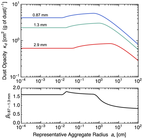
Figure 6.— Upper panel: absorption opacities $\kappa_{\rm d,\nu}$ (in units of ${\rm cm}^{2}$ per gram of dust) of dust at wavelengths $\lambda=$ 0.87 mm, 1.3 mm, and 2.9 mm as a function of the representative aggregates radius $a$. The opacities are calculated by assuming that the aggregate size distribution (not resolved in our simulation) obeys a power law $N_{\rm d}^{\prime}(a)\propto a^{-3.5}$ (Equation (20)). Lower panel: opacity slope at $\lambda=0.87$–1.3 mm versus $a_{*}$.

4.6. Dust Thermal Emission

We calculate the intensities $I_{\nu}$ of dust thermal emission at each orbital radius $r$ as

$$I_{\nu}(r)=\left[1-\exp\left(-\tau_{\nu}(r)\right)\right]B_{\nu}\left(T(r)\right),$$ (21)

where $B_{\nu}(T)$ is the Planck function,

$$\tau_{\nu}(r)=\frac{\kappa_{\rm d,\nu}(r)\Sigma_{\rm d}(r)}{\cos i}$$ (22)

is the line-of-sight optical depth, and $i$ is the disk inclination. We use $i=46.7^{\circ}$ for the HL Tau disk (ALMA Partnership et al., 2015). The Planck brightness temperature $T_{\rm B}$ is computed by solving the equation $I_{\nu}=B_{\nu}(T_{\rm B})$ for $T_{\rm B}$. Equation (22) assumes that the dust disk is geometrically thin, i.e., the radial distance over which $\kappa_{\rm d,\nu}(r)$ and $\Sigma_{\rm d}(r)$ vary is longer than the dust scale height. This assumption is, however, not always satisfied in our simulations as we discuss in detail in Section 6.3.

We will also use the flux density

$$F_{\nu}=\frac{2\pi\cos i}{d^{2}}\int_{r_{\rm in}}^{r_{\rm out}}I_{\nu}(r)rdr,$$ (23)

where $d$ is the distance to HL Tau, $r_{\rm in}=1~{}{\rm AU}$ and $r_{\rm out}=1000~{}{\rm AU}$ are the boundaries of our computational domain (see Section 4.1), and the factor $\cos i$ accounts for the ellipticity of the disk image. In accordance with ALMA Partnership et al. (2015), we set $d=140~{}{\rm pc}$, the standard mean distance to Taurus.

When comparing our simulation results with the ALMA observation, it is useful to smooth the simulated radial emission profiles at the spatial resolution of ALMA. In this study, we do this in the following two steps. First, we generate projected images of our simulation snapshots assuming the disk inclination of $46.7^{\circ}$. For simplicity, the geometrical thickness of the disks is neglected in this process. Second, we smooth the “raw” images along their major axis using a circular Gaussian with the FWHM angular resolutions of $\sqrt{85.3\times 61.1}$, $\sqrt{35.1\times 21.8}$, and $\sqrt{29.9\times 19.0}$ mas for $\lambda=2.9$, 1.3, and 0.87 mm, in accordance with the ALMA observation of HL Tau at Bands 3, 6, and 7, respectively (ALMA Partnership et al., 2015). Since we assume $d=140~{}{\rm pc}$, these angular resolutions translate into the spatial resolutions of $\approx$ 10, 3.9, and 3.3 AU at Bands 3, 6, and 7, respectively.

4.7. Parameter Sets and Initial Conditions

We conduct ten simulation runs with different sets of model parameters. Columns 1 through 4 of Table 3 list the run names and parameter choices ($\gamma$, $a_{0}$, $\alpha_{\rm t}$) for the simulation runs. Run Sa0 is our fiducial model and assumes $\gamma=1$, $a_{0}=0.1~{}\micron$, and $\alpha_{\rm t}=0.03(r/10~{}{\rm AU})^{1/2}$. Model Sa0-NoSint is the same as model Sa0 but neglects sintering. Runs Sa0-Lgam and Sa0-Hgam are designed to study the dependence of the results on the gas surface density slope $\gamma$. Runs Sa0-Lalp and Sa0-Halp will be used to study how the sintering-induced ring formation scenario constrains the radial distribution of $\alpha_{\rm t}$ in the HL Tau disk. Runs La0 and LLa0 assume more fragile aggregates (i.e., larger $a_{0}$) and weaker turbulence than in the fiducial run. As we will see, the set of $a_{0}$ and $\alpha_{\rm t}$ controls the degree of dust sedimentation, i.e., the geometrical thickness of the dust disk. Runs Sa0-tuned and La0-tuned are the same as runs Sa0 and La0, respectively, except that they adopt slightly lower $L_{j}$ for ${\rm H_{2}O}$, ${\rm NH_{3}}$, and ${\rm C_{2}H_{6}}$ (see $L_{j,\rm tuned}$ in Table 3.2). These runs will be used to quantify possible uncertainties of our results that might arise from the uncertainties in the vapor pressure data.

Table 3List of Simulation Runs

Run	$\gamma$	$a_{0}$	$\alpha_{\rm t}$	$t_{\rm snap}$	$F_{\nu}$ (Jy) at $t=t_{\rm snap}$			Section
		(µm)		(Myr)	2.9 mm	1.3 mm	0.87 mm
Sa0	$1$	$0.1$	$0.03(r/10~{}{\rm AU})^{1/2}$	0.26	0.070	0.79	2.2	5
Sa0-NoSint	$1$	0.1	$0.03(r/10~{}{\rm AU})^{1/2}$	0.12	0.063	0.79	2.3	5.5
Sa0-Lgam	$0.5$	$0.1$	$0.03(r/10~{}{\rm AU})^{1/2}$	0.29	0.076	0.76	2.1	6.1
Sa0-Hgam	$1.5$	$0.1$	$0.03(r/10~{}{\rm AU})^{1/2}$	0.05	0.072	0.80	2.3	6.1
Sa0-Lalp	$1$	$0.1$	$0.03$	0.18	0.066	0.77	2.2	6.2
Sa0-Halp	$1$	$0.1$	$0.1$	0.29	0.075	0.75	2.1	6.2
La0	$1$	1	$10^{-3}(r/10~{}{\rm AU})^{1/2}$	0.41	0.064	0.78	2.3	6.3
LLa0	$1$	4	$10^{-4}(r/10~{}{\rm AU})^{1/2}$	0.45	0.062	0.80	2.4	6.3
Sa0-tuned	$1$	0.1	$0.03(r/10~{}{\rm AU})^{1/2}$	0.27	0.068	0.77	2.2	6.4
La0-tuned	$1$	1	$10^{-3}(r/10~{}{\rm AU})^{1/2}$	0.41	0.063	0.79	2.3	6.4

The initial conditions are given by $\Sigma_{\rm d}(t=0,r)=0.01\Sigma_{\rm g}(r)$ and $a_{*}(t=0,r)=a_{0}$, where we have assumed that the dust-to-gas mass ratio of the initial disk is 0.01.

5. Results from the Fiducial Simulation

We now present the results of our simulations in the following two sections. In this section, we particularly focus on the fiducial run Sa0 and analyze its results in detail. The dependence on model parameters will be discussed in Section 6.

5.1. Evolution of the Total Dust Mass and Flux Densities

In our simulations, the observational appearance of the disk changes with time because dust particles grow and drift inward. In particular, the millimeter emission of the disk diminishes as the particles drain onto the central star. For this reason, we select from each simulation run one snapshot that best reproduces the millimeter flux densities of the HL Tau disk reported by ALMA Partnership et al. (2015). Specifically, we calculate the relative errors between the simulated and observed flux densities at $\lambda=0.87$, 1.3, and 2.9 mm as a function of time, and search for the time $t=t_{\rm snap}$ at which the sum of the relative errors is minimized. For reference, the flux densities reported by the ALMA observation are 0.0743, 0.744, and 2.14 Jy at $\lambda=0.87$, 1.3, and 2.9 mm (Bands 7, 6, and 3), respectively (ALMA Partnership et al., 2015).

Figure 7 illustrates such an analysis for our fiducial simulation run Sa0. This figure shows the simulated time evolution of the flux densities at the three wavelengths as well as the evolution of the total dust mass $M_{\rm d}$ within the computational domain. The dust mass and flux densities decrease on a timescale of $\sim 1~{}{\rm Myr}$, which reflects the timescale on which the dust near the disk’s outer edge (which dominates $M_{\rm d}$) grows into rapidly drifting pebbles (see, e.g., Sato et al., 2016). Comparing the flux densities from the simulation with those from the ALMA observations (shown by the dashed horizontal line segments in the lower panel of Figure 7), we find that the sum of the relative errors in the flux densities is minimized when $t=0.26~{}{\rm Myr}$. At this time, the flux densities in the simulation are 0.070, 0.79, and 2.2 Jy at $\lambda=$ 2.9, 1.3, and 0.87 mm, respectively, in agreement with the ALMA measurements to an accuracy of less than 6%.

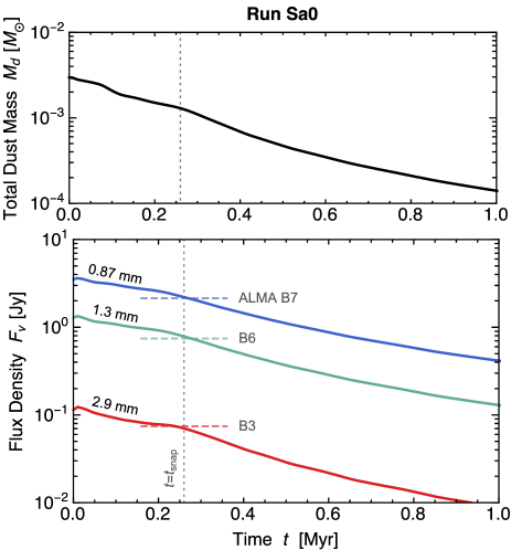
Figure 7.— Simulated time evolution of the total dust mass $M_{\rm d}$ (upper panel) and flux densities $F_{\nu}$ (lower panel) of the HL Tau disk from simulation run Sa0. The blue, green, and red solid curves in the lower panel are $F_{\nu}$ at wavelengths $\lambda=0.87$ mm, 1.3 mm, and 2.9 mm, respectively. The dashed horizontal line segments indicate the ALMA measurements of the flux densities at these wavelengths (Bands 7, 6, and 3, respectively). The vertical dotted line indicates the time $t=t_{\rm snap}$ at which the simulated flux densities best reproduce the ALMA measurements ($t_{\rm snap}=0.26~{}{\rm Myr}$ for run Sa0; see Section 5.1).

Columns 5 through 8 of Table 3 list the values of $t_{\rm snap}$ and $F_{\nu}(t=t_{\rm snap})$ for all simulation runs. We find that $t_{\rm snap}$ falls within the range $0.1$–$0.5~{}{\rm Myr}$. Since $t_{\rm snap}$ may be regarded as the time after disk formation, our results are consistent with the idea that HL Tau is younger than 1 Myr. In fact, the age predicted from our simulations depends on the disk mass $M_{\rm disk}$ assumed: a higher $M_{\rm disk}$ leads to a larger $t_{\rm snap}$ because it takes longer for dust emission to decay to the observed level when the initial dust mass is larger. However, a disk mass much in excess of $0.2~{}M_{\sun}$ seems to be unrealistic because the disk would then be gravitationally unstable at outer radii (see Section 2.2).

5.2. Aggregate Size and Dust Surface Density

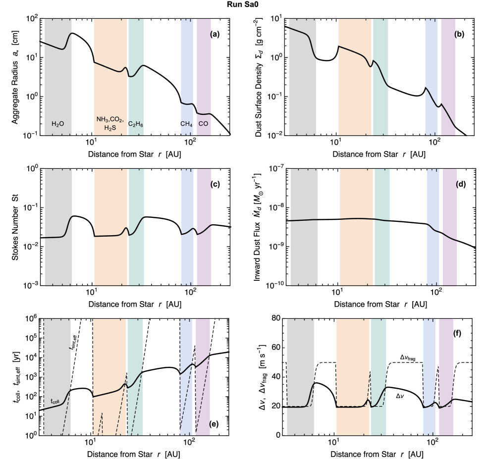
Figure 8.— Radial distribution of the representative aggregate radius $a_{*}$ (panel a), dust surface density $\Sigma_{\rm d}$ (panel b), aggregate Stokes number ${\rm St}$ (panel c), and radial inward dust flux $\dot{M}_{\rm d}$ (panel d) at time $t=t_{\rm snap}=0.26~{}{\rm Myr}$ from the fiducial simulation. The shaded areas mark the sintering zones defined by $r_{{\rm subl},j}<r<r_{{\rm subl},j}$ (see Section 3.4 for details). Panel e shows the collision timescale $t_{\rm coll}$ (Equation (12); solid line) and effective sintering timescale $t_{\rm sint,eff}$ (Equation (17); dashed line), while panel f plots the collision velocity $\Delta v$ (solid line) and fragmentation threshold $\Delta v_{\rm frag}$ (Equation (16); dashed line) for the representative aggregates.

Below we fix $t$ to be $t_{\rm snap}=0.26~{}{\rm Myr}$ and look at the radial distribution of dust in detail. Figures 8(a) and (b) show the radial distribution of the representative aggregate radius $a_{*}$ and dust surface density $\Sigma_{\rm d}$ at this time. We also show in Figure 8(c) the Stokes number ${\rm St}$ of the representative aggregates, which is more directly related to their dynamics than $a_{*}$. In these figures, the vertical stripes indicate the locations of the sintering zones. Here, the sintering zone of each volatile $j$ is defined by the locations where $r>r_{{\rm snow},j}$ and $r<r_{{\rm sint},j}$, with the latter being equivalent to $t_{\rm coll}<t_{{\rm sint},j}$ (see Figures 8(e) for the radial distribution of $t_{\rm coll}$ and $t_{\rm sint,eff}$). The sintering zones of ${\rm NH_{3}}$, ${\rm CO_{2}}$, and ${\rm H_{2}S}$ partially overlap with each other and form a single sintering zone. The exact locations of the sintering zones are 3–6 AU (${\rm H_{2}O}$), 11–23 AU (${\rm NH_{3}}$–${\rm CO_{2}}$–${\rm H_{2}S}$), 24–33 AU (${\rm C_{2}H_{6}}$), 80–106 AU (${\rm CH_{4}}$), and 116–160 AU (${\rm CO}$). Strictly speaking, the locations of the sintering zones are time-dependent because the volatile partial pressures $P_{j}$ and aggregate collision timescale $t_{\rm coll}$ evolve with $\Sigma_{\rm d}$ (see Equations (4), (5), and (12)). However, comparison between Figures 4 and 8 shows that the sintering zones little migrate during this $0.26~{}{\rm Myr}$. This is because the locations of the sintering zones depend on the radial distribution of the gas temperature $T$ (which is taken to be time-independent) much more strongly than on the distribution of $\Sigma_{\rm g}$.

Figures 8(a) and (b) show that sintering produces a clear pattern in the radial distribution of the dust component. We see that dust aggregates in the sintering zones tend to have a high surface density and a small radius compared to those in the adjacent non-sintering zones. The small aggregate size is a direct consequence of fragmentation induced by sintering. To see this, we plot in Figure 8(f) the collision velocity $\Delta v$ and fragmentation threshold $\Delta v_{\rm frag}$ as a function of $r$. In the non-sintering zones, we find $\Delta v_{\rm frag}\approx 50~{}{\rm m~{}s^{-1}}$ and $\Delta v\approx 25$–$35~{}{\rm m~{}s^{-1}}$, implying that no disruptive collisions occur for the unsintered aggregates (as we will see below, the maximum size of the unsintered aggregates is determined by radial drift rather than by fragmentation). In the sintering zones, $\Delta v_{\rm frag}$ is decreased to $20~{}{\rm m~{}s^{-1}}$, and $\Delta v$ is also suppressed down to the same value. Since $\Delta v$ is an increasing function of $a_{*}$ (as long as ${\rm St}\ll 1$), this indicates that the sintered aggregates disrupt each other so that $\Delta v$ never exceeds $\Delta v_{\rm frag}$. The disrupted aggregates pile up there because the inward drift speed $|v_{\rm r}|$ decreases with decreasing $a_{*}$. These pileups provide the high surface densities in the sintering zones.

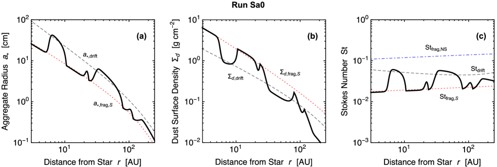
Figure 9.— Same as panels (a), (b), and (c) of Figure 8 but compared with the analytic estimates assuming steady inward dust flow ($\dot{M}_{\rm d}=5\times 10^{-9}~{}{M}_{\odot}~{}{\rm yr}^{-1}$). The dashed curves show the drift-limited solution for unsintered aggregates (labeled by “NS”), while the dotted curves the fragmentation-limited solution of sintered aggregates (labeled by “S”).

To understand the radial distribution of $\Sigma_{\rm d}$ and $a_{*}$ more quantitatively, we now look at the radial inward mass flux of drifting aggregates,

$$\dot{M}_{\rm d}\equiv 2\pi r|v_{\rm r}|\Sigma_{\rm d}.$$ (24)

The radial distribution of $\dot{M}_{\rm d}$ is shown in Figure 8(d). We can see that the mass flux is radially constant ($\approx 5\times 10^{-9}~{}M_{\sun}~{}{\rm yr}^{-1}$) at $\lesssim 100~{}{\rm AU}$. This indicates that the radial dust flow in this region can be approximated by a steady flow. Such a quasi-steady dust flow is commonly realized when some mechanism like radial drift or fragmentation limits dust growth (see, e.g., Birnstiel et al., 2012; Lambrechts & Johansen, 2014). Substituting $|v_{\rm r}|\approx 2\eta v_{\rm K}{\rm St}$ (${\rm St}\ll 1$) into Equation (24), we obtain the relation between $\Sigma_{\rm d}$ and ${\rm St}$,

$$\Sigma_{\rm d}=\frac{\dot{M}_{\rm d}}{2\pi r|v_{\rm r}|}\approx\frac{\dot{M}_{\rm d}}{4\pi\eta rv_{\rm K}{\rm St}}.$$ (25)

Since ${\rm St}\propto a_{*}$, we have $\Sigma_{\rm d}\propto 1/a_{*}$ for constant $\dot{M}_{\rm d}$.

Using Equation (25) together with the assumption that either radial drift or fragmentation limits dust growth, one can estimate the radial distribution of $\Sigma_{\rm d}$ and $a_{*}$ in the non-sintering and sintering zones in an analytic way. When radial drift limits dust growth, the maximum aggregate size is determined by the condition (Okuzumi et al., 2012)

$$\frac{t_{\rm coll}}{t_{\rm drift}}\approx\frac{1}{30},$$ (26)

where $t_{\rm coll}$ is the collision timescale already given by Equation (12) and

$$t_{\rm drift}\equiv\frac{r}{|v_{\rm r}|}\approx\frac{1}{2\eta\Omega{\rm St}}$$ (27)

is the timescale of radial drift. Substituting $H_{\rm d}\approx(1+{\rm St}/\alpha_{\rm t})^{-1/2}H_{\rm g}$ (${\rm St}\ll 1$) and $m_{*}/\pi a_{*}^{2}=(4/3)\rho_{\rm int}a_{*}=(8/3\pi)\Sigma_{\rm g}{\rm St}$ into Equation (13), the collision timescale can be evaluated as

$$t_{\rm coll}\approx 0.53\frac{\Sigma_{\rm g}}{\Sigma_{\rm d}}\frac{H_{\rm g}{\rm St}}{\Delta v\sqrt{1+{\rm St}/\alpha_{\rm t}}}$$ (28)

Furthermore, the collision velocity can be approximated as the root square sum of the turbulence-driven velocity $\Delta v_{\rm t}$ and differential radial drift velocity $\Delta v_{\rm r}$,

$$\Delta v\approx\sqrt{(\Delta v_{\rm t})^{2}+(\Delta v_{\rm r})^{2}}\approx\sqrt{2.3\alpha_{\rm t}c_{\rm s}^{2}{\rm St}+(\eta v_{\rm K}{\rm St})^{2}},$$ (29)

where we have used the approximate expressions for $\Delta v_{\rm t}$ and and $\Delta v_{\rm r}$ already given in Section 4.3. Substituting Equations (25) and (27)–(29) into Equation (26), we obtain the equation for the maximum Stokes number in the drift-limited growth,

$$\frac{{\rm St}_{\rm drift}^{5/2}}{\sqrt{(2.3\alpha_{\rm t}c_{\rm s}^{2}+\eta^{2}v_{\rm K}^{2}{\rm St}_{\rm drift})(1+{\rm St}_{\rm drift}/\alpha_{\rm t})}}=\frac{0.0025\dot{M}_{\rm d}}{\eta^{2}rv_{\rm K}c_{\rm s}\Sigma_{\rm g}},$$ (30)

where we have labeled ${\rm St}$ by the subscript “drift” to emphasize drift-limited growth. In Figure 9(c), we compare ${\rm St}_{\rm drift}$ for $\dot{M}_{\rm d}=5\times 10^{-9}~{}M_{\sun}~{}{\rm yr}^{-1}$ with the Stokes number directly obtained from run Sa0 at $t=t_{\rm snap}$. We find that ${\rm St}_{\rm drift}$ reproduces ${\rm St}$ in the non-sintering zones, implying that radial drift limits the growth of unsintered aggregates. We are also able to estimate $a_{*}$ and $\Sigma_{\rm d}$ in the non-sintering zones by substituting ${\rm St}={\rm St}_{\rm drift}$ into $a_{*}=(2/\pi)\Sigma_{\rm g}{\rm St}/\rho_{\rm int}$ and Equation (25), respectively. These are shown by the dashed lines in Figures 9(a) and (b).

If fragmentation limits dust growth, the maximum Stokes number is simply determined by the balance

$$\Delta v({\rm St})=\Delta v_{\rm frag}.$$ (31)

We will denote the solution to this equation by ${\rm St}_{\rm frag}$. If we approximate $\Delta v$ by Equation (29), Equation (31) can be rewritten as a quadratic equation for ${\rm St}$, and its positive root gives

$${\rm St}_{\rm frag}=\frac{-2.3\alpha_{\rm t}c_{\rm s}^{2}+\sqrt{(2.3\alpha_{\rm t}c_{\rm s}^{2})^{2}+4(\eta v_{\rm K}\Delta v_{\rm frag})^{2}}}{2(\eta v_{\rm K})^{2}}.$$ (32)

The dot-dashed and dotted lines in Figure 9(c) show ${\rm St}_{\rm frag}$ for $\Delta v_{\rm frag}=\Delta v_{\rm frag,NS}$ and $\Delta v_{\rm frag,S}$ (denoted by ${\rm St}_{\rm frag,NS}$ and ${\rm St}_{\rm frag,S}$), respectively. We can see that ${\rm St}_{\rm frag,S}$ reproduces ${\rm St}$ in the sintering zones, which confirms that fragmentation limits the growth of sintered aggregates. One can estimate the values of $a_{*}$ and $\Sigma_{\rm d}$ in the sintering zones by substituting ${\rm St}={\rm St}_{\rm frag,S}$ into $a_{*}=2\Sigma_{\rm g}{\rm St}/(\pi\rho_{\rm int})$ and Equation (25). These estimates are in excellent agreement with the simulation results as shown by the dotted lines of Figures 9(a) and (b).

5.3. Lifetime of the Ring Patterns

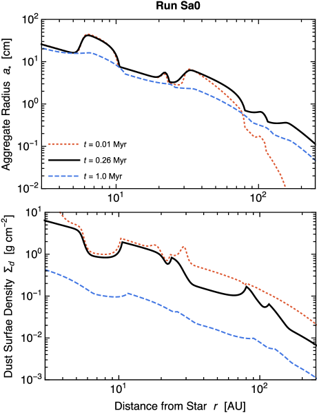
Figure 10.— Radial distribution of the representative aggregate radius $a$ (upper panel) and dust surface density $\Sigma_{\rm d}$ (lower panel) at $t=0.01~{}{\rm Myr}$ (dotted lines), $0.26~{}{\rm Myr}$ (solid lines), and $1~{}{\rm Myr}$ (dashed line) from simulation run Sa0.

It is worth mentioning at this point that the radial pattern of dust as shown in Figure 8 fades out as the disk becomes depleted of dust. As the dust-to-gas mass ratio $\Sigma_{\rm d}/\Sigma_{\rm g}$ decreases, the collision timescale $t_{\rm coll}$ of the aggregates increases, and consequently the maximum aggregate size set by radial drift (Equation (26)) decreases. the radial pattern disappears when the radial drift barrier dominates over the fragmentation barrier at all $r$ because sintering has no effect on radial drift. This is illustrated in Figure 10, where we plot the radial distribution of $a_{*}$ and $\Sigma_{\rm d}$ for model Sa0 at different values of $t$. We find that the radial pattern that was present at $t=t_{\rm snap}=0.26~{}{\rm Myr}$ has disappeared by $t=1~{}{\rm Myr}$. In this particular example, ${\rm St}_{\rm drift}$ falls below ${\rm St}_{\rm frag,S}$ at all $r$ when ${M}_{\rm d}<10^{-11}~{}M_{\sun}~{}{\rm yr}^{-1}$. In models La0 and LLa0, which assume weaker turbulence, dust evolution is slower than in model Sa0 owing to the lower turbulence-driven collision velocity (see $t_{\rm snap}$ in Table 3). However, even in these cases, the sintering-induced ring patterns are found to decay in 2 Myr. We note that the lifetime of the pattern would be longer for radially more extended ($r_{\rm c}>150~{}{\rm AU}$) disks, because the lifetime of dust flux in a disk generally scales with the orbital period at the disk’s outer edge (Sato et al., 2016).

5.4. Optical Depths and Brightness Temperatures

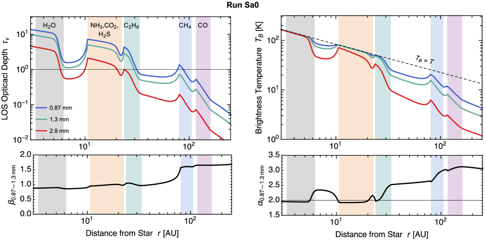
Figure 11.— Radial distribution of the line-of-sight optical depths $\tau_{\nu}$ (upper left panel), brightness temperatures $T_{\rm B}$ (upper right panel), opacity slope $\beta_{\rm 0.87\textrm{--}1.3~{}mm}$ (lower left panel), and spectral slope $\alpha_{\rm 0.87\textrm{--}1.3~{}mm}$ (lower right panel) at $t=t_{\rm snap}=0.26~{}{\rm Myr}$ from run Sa0. The blue, green, and red curves in the upper panels correspond to wavelengths $\lambda=$ 0.87, 1.3, and 2.9 mm (ALMA Bands 7, 6, and 3), respectively. The dashed line in the upper right panel shows the gas temperature profile $T$ in our disk model (Equation (1)). The shaded areas mark the sintering zones.

We move on to the observational appearance of the sintering-induced dust rings at millimeter wavelengths. The upper left panel of Figure 11 shows the radial distribution of the line-of-sight optical depths $\tau_{\nu}$ (Equation (22)) from the snapshot of run Sa0 at $t=t_{\rm snap}$. We here present the optical depths at three wavelengths $\lambda=$ 0.87, 1.3, and 2.9 mm, which correspond to ALMA Bands 7, 6, and 3, respectively.

Overall, the optical depths in the sintering zones are higher than in the non-sintering zones. This mainly reflects the higher dust surface density in the sintering zones (see Figure 8(b)). The radial variation of $\kappa_{{\rm d},\nu}$ represents only a minor contribution to the radial variation of $\tau_{\nu}$, in particular in outer regions where the representative aggregates are smaller than $\sim 1~{}{\rm cm}$ in radius. At $\lambda=$ 0.87 and 1.3 mm, the three inner sintering zones (of ${\rm H_{2}O}$, ${\rm NH_{3}}$–${\rm CO_{2}}$–${\rm H_{2}S}$, and ${\rm C_{2}H_{6}}$) are optically thick, while the two outer sintering zones (of ${\rm CH_{4}}$ and ${\rm CO}$) are optically thin or marginally thick. The ${\rm CO}$ sintering zone is much darker than the other sintering zones because the disk surface density drops at $r>r_{\rm c}=150~{}{\rm AU}$. The non-sintering zones are optically thin or marginally thick at all three wavelengths. The opacity index at $\lambda=$ 0.87–1.3 mm, $\beta_{\rm 0.87\textrm{--}1.3~{}mm}\equiv{\ln(\kappa_{\rm 0.87~{}mm}/\kappa_{\rm 1.3~{}mm})}/{\ln(\nu_{\rm 0.87~{}mm}/\nu_{\rm 1.3~{}mm})}$ is shown in the lower left panel of Figure 11. We see that $\beta_{\rm 0.87\textrm{--}1.3~{}mm}\sim 1$ at $\lesssim 70~{}{\rm AU}$ and approaches the interstellar value $\sim 1.7$ beyond 80 AU.

The upper right panel of Figure 11 shows the distribution of the brightness temperatures $T_{\rm B}$ for the same snapshot. For comparison, we also plot the gas temperature $T$ of our disk model given by Equation (1). We find that the three innermost sintering zones are optically thick ($T_{\rm B}\approx T$) at $\lambda=$ 0.87 mm and 1.3 mm.

An interesting observational signature of the sintering-induced rings appears in the radial variation of the spectral slope. In the lower right panel of Figure 11, we plot the spectral index at 0.87–1.3 mm, $\alpha_{\rm 0.87\textrm{--}1.3~{}mm}\equiv\ln(I_{\rm 0.87~{}mm}/I_{\rm 1.3~{}mm})/\ln(\nu_{\rm 0.87~{}mm}/\nu_{\rm 1.3~{}mm})$, as a function of $r$. In the three innermost sintering zones, we have $\alpha_{\rm 0.87\textrm{--}1.3~{}mm}\approx 2$ since these zones are optically thick at these wavelengths. If these regions were optically thin, we would have $\alpha_{\rm 0.87\textrm{--}1.3~{}mm}\approx 3$ because $\beta_{\rm 0.87\textrm{--}1.3~{}mm}\approx 1$ (see the lower left panel of Figure 11). In the non-sintering zones lying at $\sim$ 6–11 AU and $\sim$ 33–80 AU, we obtain $\alpha_{\rm 0.87\textrm{--}1.3~{}mm}\approx 2.3$–2.5, which is in between the values in the optically thick and thin limits. This reflects the fact that the non-sintering zones are marginally thick at 0.87–1.3 mm.

5.5. Comparison with the ALMA Observation

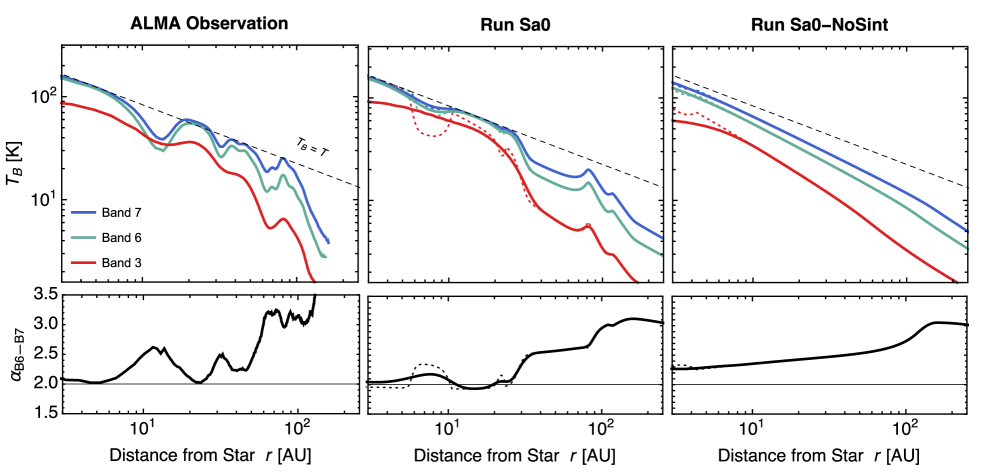
Figure 12.— Comparison between the ALMA observation and our fiducial model calculation Sa0. The left panels show the radial profiles of $T_{\rm B}$ at Bands 3, 6, and 7 and $\alpha_{\rm B6\textrm{--}B7}$ of the HL Tau disk obtained from the ALMA observation (same as Figure 1). The center and right panels are from simulation runs Sa0 and Sa0-NoSint. The simulated profiles are obtained by smoothing the raw simulation data (dotted curves) at the ALMA resolutions (see text for details). The dashes lines show $T_{\rm B}=T$, where $T$ is the gas temperature given by Equation (1).

Now we make more detailed comparisons between the simulation results and the ALMA observation of the HL Tau disk. We here smooth the radial profiles of the intensities $I_{\nu}$ from run Sa0 ($t=t_{\rm snap}$) at the ALMA resolutions as described in Section 4.6. In the center panels of Figure 12, the solid lines show the radial profiles of the brightness temperatures $T_{\rm B}$ and spectral slope $\alpha_{\rm B6\textrm{--}B7}$ obtained from the smoothed $I_{\nu}$. For comparison, $T_{\rm B}$ and $\alpha_{\rm B6\textrm{--}B7}$ from the raw $I_{\nu}$ are shown by the dotted lines. The left panels show the profiles from the ALMA observations (same as Figure 1). We also show in the right panels the results from the no-sintering run Sa0-NoSint to clarify the features of the sintering-indued structures.

After smoothing, the innermost emission dip lying at 6–11 AU has been partially smeared at 0.87 mm (Band 7) and 1.3 mm (Band 6). The emission dip in the smoothed images has a lower spectral slope than that in the raw images directly obtained from the simulation. This is a consequence of the frequency-dependent angular resolution: since Band 6 has a coarser resolution than Band 7, the emission dip seen at Band 6 is more significantly buried than that seen at Band 7, resulting in a decrease in the spectral slope after smoothing. At 2.9 mm (Band 3), the radial structure of $T_{\rm B}$ at $\lesssim 10$ AU has been significantly smoothed out.

We find that our simulation reproduces many observational features of the HL Tau disk. First, the simulation predicts a central emission peak that closely resembles the observed one. This central emission peak is associated with the ${\rm H_{2}O}$ sintering zone as shown in Figure 11. The radial extent of the simulated central peak is $\approx 6~{}{\rm AU}$, which is comparable to $\approx 8~{}{\rm AU}$ of the observed peak. The simulation perfectly reproduces the emission features of the central region: the magnitudes and radial slopes of $T_{\rm B}$ at all three ALMA Bands, and the millimeter spectral slope of $\alpha_{\rm B6\textrm{--}B7}\approx 2$. In our simulation, the spectral slope simply reflects the high optical thickness of the central region, having nothing to do with the optical properties of the aggregates in the region. Sintering plays an essential role in the buildup of the optically thick region; without sintering, the disk would be entirely optically thin at these bands as shown by run Sa0-NoSint (see the right panels of Figure 12). The fact that the central emission peak has a lower intensity at Band 3 than at Bands 6 and 7 is explained as a consequence of the lower spatial resolution ($\approx 10~{}{\rm AU}$) at Band 3, i.e., this compact emission is underresolved at this band.

The simulation also predicts two bright rings in the region of $\sim$ 10–30 AU that might be identified with the two innermost bright rings of HL Tau observed at $\sim 20~{}{\rm AU}$ and 40 AU. In our simulation, the two emission rings are associated with the sintering zones of ${\rm NH_{3}}$–${\rm CO_{2}}$–${\rm H_{2}S}$ (11–23 AU) and ${\rm C_{2}H_{6}}$ (24–33 AU). These rings are optically thick at Bands 6 and 7 (and therefore $\alpha_{\rm B6\textrm{--}B7}\approx 2$) and are optically thin at Band 3. These features are consistent with those of the two innermost bright rings of HL Tau. However, the separation of the predicted rings are much smaller than in the observed rings as we discuss below.

Farther out in the disk, the simulation predicts an optically thin emission peak at 80 AU associated with ${\rm CH_{4}}$ sintering. Its location coincides with the 80 AU bright ring in the ALMA image of HL Tau, and its brightness temperatures agree with those of the observed ring at all three wavelengths to within a factor of two. The simulation also predicts a less pronounced peak at 120 AU associated with ${\rm CO}$ sintering. As mentioned in Section 5.4, this 120 AU peak is much less pronounced than other inner peaks because this location is close to the outer edge of our modeled gas disk. Interestingly, the observed HL Tau disk also has one minor emission peak exterior to the 80 AU ring ($r\sim 97~{}{\rm AU}$; see ALMA Partnership et al. 2015).

The innermost dark ring seen at 6–11 AU in the simulated image is optically marginally thick and has $\alpha_{\rm B6\textrm{--}B7}>2$, consistent with the observed innermost dark ring at $\sim 13~{}{\rm AU}$. Our simulation also explains why this innermost emission dip is much shallower at Band 3 than at Bands 6 and 7: as mentioned above, this is simply because the spatial resolution at Band 3 is no high enough to distinguish the dark ring from the central emission peak.

However, there are some discrepancies between the prediction from the fiducial model and the observation of the HL Tau disk. For example, the second innermost ring predicted by the model, which is associated with the ${\rm C_{2}H_{6}}$ sintering zone, is about 10 AU interior to that observed by ALMA. For this reason, the dark ring just inside the ${\rm C_{2}H_{6}}$ sintering zone is much narrower than the second innermost dark ring of HL Tau extending from 30 AU to 40 AU. In addition, as we explain in detail in Section 6.3, the fiducial model predicts that dust particles are vertically well mixed in the gas disk, which seems to be inconsistent with the observations of HL Tau suggesting that large dust particles settle to the disk midplane (Kwon et al., 2011; Pinte et al., 2016). In the following section, we will examine if these discrepancies can be removed or alleviated by tuning the parameters in our model.

6. Parameter Study

The previous section has mainly focused on our fiducial simulation (run Sa0). We here study how the simulation results depend on the model parameters.

6.1. Gas Surface Density Slope

Since the gas density distribution of the HL Tau disk is unknown, it is important to quantify how strongly our results depend on the assumption about the gas density profile. We here present the results of two simulation runs Sa0-Lgam and Sa0-Hgam, in which we vary $\gamma$ in Equation (2) to 0.5 and 1.5, respectively. The other parameters are unchanged form the fiducial run.

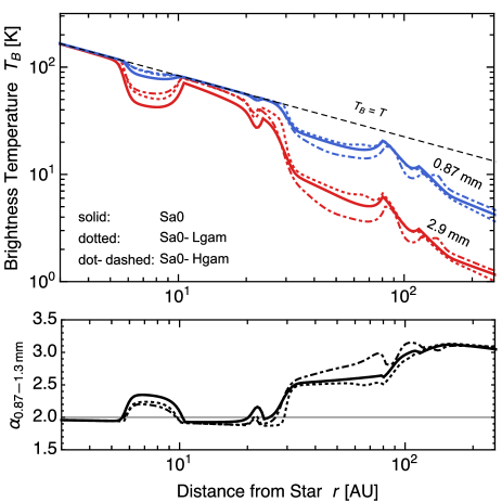
Figure 13.— Comparison between runs Sa0 (solid curves), Sa0-Lgam (dotted curves), Sa0-Hgam (dot-dashed curves). The upper panel shows the brightness temperatures $T_{\rm B}$ as a function of orbital distance $r$ at wavelengths 0.87 mm (blue curves) and 2.9 mm (red curves) at time $t=t_{\rm snap}$. The gas temperature profile $T$ (Equation (1)) is shown by the dashed line. The lower panel shows the opacity index at 0.87–1.3 mm.

Figure 13 compares the radial profiles of the brightness temperature and spectral slope at 0.87 mm and 2.9 mm from these runs with those from run Sa0. The three snapshots are taken at different times but still provide similar flux densities (see Table 3) because $t_{\rm snap}$ is defined as such. We find that the variation of $\gamma$ within the range 0.5–1.5 little affects the emission properties of the disk, with the variation of $T_{\rm B}$ within a factor of 2 and the variation of $\alpha_{\rm 0.87\textrm{--}1.3~{}mm}$ as small as $\lesssim 25\%$ at all $r$. This is mainly because the steady-state radial distribution of the dust surface density $\Sigma_{\rm d}$ is insensitive to $\gamma$. If we measure the aggregate size by St, the steady-state distribution of $\Sigma_{\rm d}$ is determined from Equation (25) with either ${\rm St}={\rm St}_{\rm drift}$ (Equation (30)) or ${\rm St}={\rm St}_{\rm frag}$ (Equation (32)). The $\gamma$ dependence of the radial dust flux $\dot{M}_{\rm d}$ is weak as long as we fix $M_{\rm disk}$ and $r_{\rm c}$. ${\rm St}_{\rm frag}$ depends on $\gamma$ only through $\eta\propto\gamma+1.8$ (for $T\propto r^{-0.57}$ and $r\ll r_{\rm c}$), and its variation is small as long as we vary $\gamma$ within the range 0.5–1.5. For ${\rm St}_{\rm drift}$, the dependence is less obvious from Equation (30), but it turns out that the weak $\gamma$ dependences of $\eta^{2}\Sigma_{\rm d}$ and $\dot{M}_{\rm d}$ partly cancel out in this equation.

6.2. Radial Variation of Turbulence

The radial distribution of turbulence strength $\alpha_{\rm t}$ is another important uncertainty in our simulations. Our fiducial model assume $\alpha_{\rm t}\propto\sqrt{r}$, which gives a turbulence-driven collision velocity nearly independent of $r$ ($\Delta v_{\rm t}\propto\sqrt{\alpha_{\rm t}}c_{\rm s}\propto\sqrt{\alpha_{\rm t}T}\propto r^{-0.035}$). In fact, a radially constant collision velocity is required in our model to simultaneously reproduce dark rings at small $r$ and bright rings at large $r$ simultaneously. To demonstrate this, we here consider two models in which $\alpha_{\rm t}$ is fixed to 0.03 and 0.1 at all $r$ (referred as models Sa0-Lalp and Sa0-Halp, respectively). These values correspond to the values of $\alpha_{\rm t}$ in the fiducial Sa0 model at $r\approx 10~{}{\rm AU}$ and $100~{}{\rm AU}$, respectively.

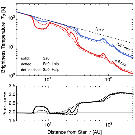
Figure 14.— Comparison between runs Sa0 (solid curves), Sa0-Lalp (dotted curves), Sa0-Halp (dot-dashed curves). The upper panel shows the brightness temperatures $T_{\rm B}$ as a function of orbital distance $r$ at wavelengths 0.87 mm (blue curves) and 2.9 mm (red curves) at time $t=t_{\rm snap}$. The gas temperature profile $T$ (Equation (1)) is shown by the dashed line. The lower panel shows the opacity index at 0.87–1.3 mm.

Figure 14 compares the result of fiducial run Sa0 with those of runs Sa0-Lalp and Sa0-Halp. We find that model Sa0-Lalp fails to produce an emission peak at $\approx 80~{}{\rm AU}$. This is because turbulence is too weak to cause fragmentation of sintered aggregates at that location. By contrast, model Sa0-Halp produces only shallow dips at $r\lesssim 30~{}{\rm AU}$. In this high-$\alpha_{\rm t}$ model, the maximum aggregate size at $r\lesssim 30~{}{\rm AU}$ is limited by turbulent fragmentation even in the non-sintering zones. The suppressed dust growth causes a slowdown of radial drift, which acts to fill the density dips in the non-sintering zones. Thus, a model assuming a high $\alpha_{\rm t}$ in outer regions and a low $\alpha_{\rm t}$ in inner regions best reproduces the observation of HL Tau.

Theoretically, $\alpha_{\rm t}$ that is lower at smaller $r$ has been expected for turbulence driven by the magnetorotational instability (MRI; Balbus & Hawley, 1991). Since the origin of the MRI is the coupling between the gas disk and magnetic fields, MRI turbulence tends to be weaker at locations where the ionization degree is lower. In protoplanetary disks, a lower ionization degree corresponds to a higher gas density and hence to a smaller orbital radius, because ionizing cosmic-rays or X-rays are attenuated at large column densities and because recombination is faster in denser gas (e.g., Sano et al., 2000; Bai, 2011).

6.3. Monomer Size and Dust Settling

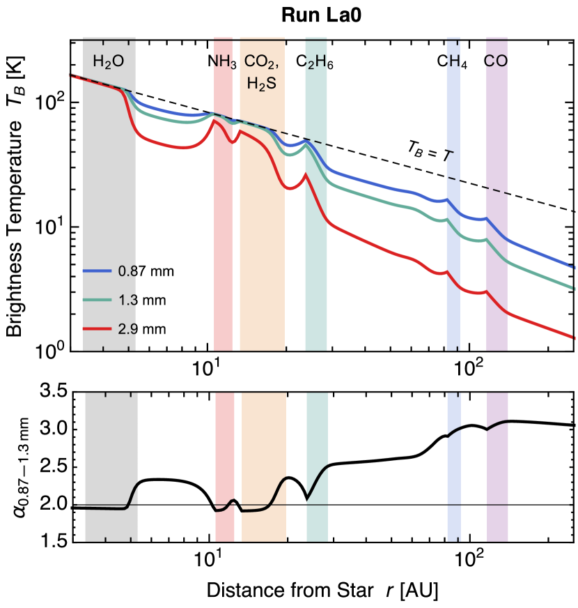
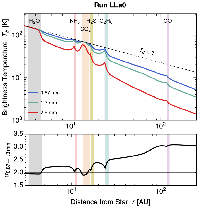
Figure 15.— Same as the right panels of Figure 11 but for models La0 (left panels) and LLa0 (right panels).

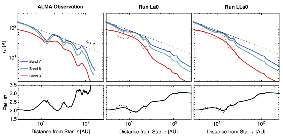
Figure 16.— Same as Figure 12, but for models La0-tuned (center panels) and LLa0-tuned (right panels).

As mentioned in Section 4.6, our calculations of dust thermal emission neglect the geometrical thickness of the dust subdisk. In reality, if a dust disk has an inclination of $\sim 45^{\circ}$ and a finite vertical extent $H_{\rm d}$, any radial structure of the disk emission is smeared out over this length scale in the direction of the minor axis of the disk image. Pinte et al. (2016) point out that the scale height of large dust particles in the HL Tau disk must be as small as $\sim 1~{}{\rm AU}$ at $r=100~{}{\rm AU}$ in order to be consistent with the well separated morphology of the bright rings observed by ALMA. Such a small dust scale height strongly indicates that dust settling has occurred in the gas disk; without settling, the dust scale height would be $\sim 10~{}{\rm AU}$ at 100 AU.

However, in our fiducial model, the settling of representative aggregates is severely prevented by turbulent diffusion. According to Equation (14), significant settling of dust particles ($H_{\rm d}\ll H_{\rm g}$) requires ${\rm St}\gg\alpha_{\rm t}$. This condition is not satisfied in fiducial run Sa0, because the value of ${\rm St}$ of the representative aggregates observed in the simulation is comparable to the value of $\alpha_{\rm t}$ assumed (see Figure 8(c)). In this run, $\alpha_{\rm t}$ is arranged to have a high value so that aggregates disrupt and pile up in the sintering zones. If turbulence were weak, sintered aggregates would not experience disruption as long as we maintain the assumption $\Delta v_{\rm frag,S}=20~{}{\rm m~{}s^{-1}}$.

One way to reconcile sintering-induced ring formation with dust settling in our model is to assume weaker turbulence and a lower fragmentation velocity. Within our dust model, a lower value of $\Delta v_{\rm frag}$ corresponds to a larger monomer size $a_{0}$ (see Equations (18) and (19)). However, aggregates made of larger monomers tend to be sintered less slowly as demonstrated in Section 3.4. To examine if there is a range of $a_{0}$ where the aggregates can experience settling and sintering simultaneously, we performed two simulations named La0 and LLa0. In run La0, we increase $a_{0}$ to $1~{}\micron$ while lowering $\alpha_{\rm t}$ to $10^{-3}(r/10~{}{\rm AU})^{1/2}$. Run LLa0 is a more extreme case of $a_{0}=4~{}\micron$ and $\alpha_{\rm t}=10^{-4}(r/10~{}{\rm AU})^{1/2}$. The other parameters are the same as in the fiducial run Sa0.

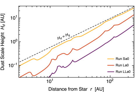
Figure 17.— Dust scale height $H_{d}$ versus orbital radius $r$ at time $t=t_{\rm snap}$ for runs Sa0 (black curve) and La0 (dashed curve). The dashed line shows the gas scale height $H_{\rm g}$.

Figure 15 shows the raw radial profiles of $T_{\rm B}$ and 0.87–1.3 mm spectral index at $t=t_{\rm snap}$ obtained from runs La0 and LLa0. The profiles after smoothing at the ALMA resolutions are shown in Figure 16. Note again that we neglect the geometric thickness of the dust disk when calculating $T_{\rm B}$. Indeed, the dust disks in models La0 and LLa0 are geometrically thin unlike in model Sa0 because turbulent diffusion is inefficient in these two models. We plot in Figure 17 the dust scale height $H_{\rm d}$ from Equation (14) as a function of $r$ for the three models. At $r=100~{}{\rm AU}$, we find $H_{\rm d}\approx 3~{}{\rm AU}$ for model La0 and $H_{\rm d}\approx 1~{}{\rm AU}$ for model LLa0. Models Sa0, La0 and LLa0 give similar results for the radial distribution of $T_{\rm B}$, particularly in inner disk regions. However, model LLa0 fails to produce an emission peak at 80 AU because the ${\rm CH_{4}}$ sintering zone completely disappears for $a_{0}=4~{}\micron$.

In summary, we find that dust settling gives a strong constraint on the turbulence strength and monomer grain size in the HL Tau disk. Dust settling and pileup occur simultaneously only if $10^{-4}<\alpha_{\rm t}\lesssim 10^{-3}$ and $1~{}\micron\lesssim a_{0}<4~{}\micron$. If $a_{0}\gtrsim 4~{}\micron$, sintering would be too slow to provide an appreciable emission peak at $\sim 80~{}{\rm AU}$. If $a_{0}\ll 1~{}\micron$, sintered aggregates would be disrupted only when $\alpha_{\rm t}\gg 10^{-3}$, but such a strong turbulence would inhibit dust settling.

Interestingly, the above results suggest the grains constituting the aggregates in the HL Tau disk are considerably larger than interstellar grains ($\lesssim 0.25~{}\micron$ in radius; e.g, Mathis et al. 1977). They are also larger than grains constituting interplanetary dust particles of presumably cometary origin (typically 0.1–0.5 $\micron$ in diameter; e.g., Rietmeijer 1993). However, such a large grain size is not excluded by the previous observations of HL Tau. The near-infrared scattered light images of the envelope of HL Tau are best reproduced by models that assume the maximum particle size of more or less $1~{}\micron$ (Lucas et al., 2004; Murakawa et al., 2008). Since the scattered light probes the envelope’s surface layer where coagulation is inefficient, the observed micron-sized particles might be monomers rather than aggregates.

6.4. Sublimation Energies

As mentioned in Section 5.5, the fiducial model does not fully explain the exact locations and widths of all major HL Tau rings. For example, the innermost dark ring predicted by model Sa0 lies somewhat closer to the central star than the observed one. If we define the position of the innermost dark ring as the location where $T_{\rm B}/T$ at Band 6 is maximized, the radius of the predicted innermost dark ring (8 AU) is $\approx 40$% smaller than that of the observed one (13 AU). Furthermore, the second innermost dark ring in model Sa0 is much narrower than that observed because the ${\rm C_{2}H_{6}}$ snow line lies very close to the ${\rm H_{2}S}$ sintering line. Of course, a different temperature profile would provide a different configuration of the sintering zones. However, as long as $T(r)$ is assumed to obey a single power law, it is generally impossible to move some of the sintering zones while unchanging the positions of the others. For example, a temperature profile slightly higher than Equation (1) would shift the ${\rm C_{2}H_{6}}$ sintering zone to 40 AU, but would at the same time shift the ${\rm CH_{4}}$ sintering zone to 100 AU. Moreover, a different $T(r)$ would make our prediction for the brightness temperatures in the optically thick regions less good.

However, the locations of the sintering zones depend not only on the gas temperature profile but also on the sublimation energies $L_{j}$ in $P_{{\rm ev},j}(T)$. As mentioned in Section 3.2, there is typically a $10\%$ uncertainty in the published data of $L_{j}$. In general, a 10% uncertainty in the sublimation energy causes a $\sim 10\%$ uncertainty in the sublimation temperature $T_{{\rm subl},j}$ because $P_{{\rm ev},j}$ is a function of the ratio $L_{j}/T$. Assuming the temperature profile given by Equation (1), we have $r_{{\rm snow},j}\propto T_{{\rm subl},j}^{-1.8}$ and hence $|\delta r_{{\rm snow},j}|/r_{{\rm snow},j}\approx 1.8|\delta T_{{\rm subl},j}|/T_{{\rm subl},j}\sim 2|\delta L_{j}|/L_{j}$, where $\delta L_{j}$, $\delta T_{{\rm subl},j}$, and $\delta r_{{\rm snow},j}$ denote the uncertainties of $L_{j}$, $T_{{\rm subl},j}$, and $r_{{\rm snow},j}$, respectively. Consequently, a $10\%$ uncertainty in $L_{j}$ leads to a $\sim 20\%$ uncertainty in the snow line location. Such an uncertainty can be significant because the separations of the observed rings are only a fraction of their radii.

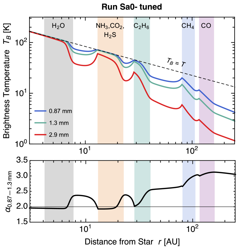
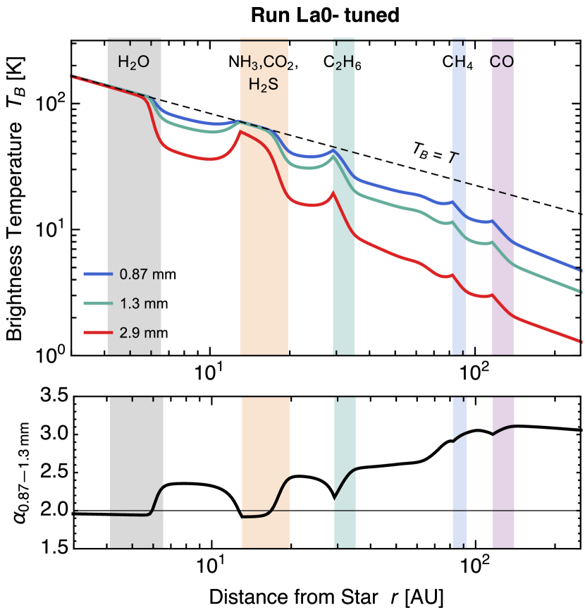
Figure 18.— Same as the right panels of Figure 11 but for runs Sa0-tuned (left panels) and La0-tuned (right panels).

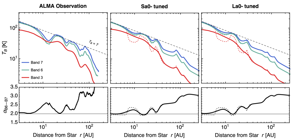
Figure 19.— Same as Figure 12, but for models Sa0-tuned (center panels) and La0-tuned (right panels), which adopt optimized sublimation energies for ${\rm H_{2}O}$, ${\rm NH_{3}}$, and ${\rm C_{2}H_{6}}$.

To demonstrate the potential importance of uncertainties in the sublimation energies, we performed two simulations named Sa0-tuned and La0-tuned. The parameters adopted in these simulations are the same as those in Sa0 and La0, respectively, except that the sublimation energies of ${\rm H_{2}O}$, ${\rm NH_{3}}$, and ${\rm C_{2}H_{6}}$ are lowered by 10% from our baseline values (see column 5 of Table 3.2). According to the estimate shown above, such modifications shift the sintering zones of these volatiles outward by $\sim 20\%$. The resulting radial profiles of $T_{\rm B}$ and $\alpha_{\rm 0.87\textrm{--}1.3~{}mm}$ before smoothing are shown in Figure 18. In model Sa0-tuned, the three innermost sintering zones are located at 4–8 AU (${\rm H_{2}O}$), 13–23 AU (${\rm NH_{3}}$–${\rm CO_{2}}$–${\rm H_{2}S}$), and 29–40 AU (${\rm C_{2}H_{6}}$) instead of 3–6 AU, 11–23 AU, and 24–33 AU as in model Sa0. Figure 19 shows the radial emission profiles after smoothing, which we compare with the ALMA observation. For the sake of comparison, we define the radii of the bright and dark rings by the orbital radii at which $T_{\rm B}/T$ at Band 6 is locally maximized and minimized, respectively. Then, the radii of four innermost bright/dark rings are found to be 13, 23, 32, and 38 AU for the observation, 9, 16, 24, and 30 AU for model Sa0-NoSint, and 9, 15, 24, and 29 AU for model La0-NoSint. Thus, model Sa0-NoSint reproduces the ring radii in the observed image to an accuracy of $\lesssim 30\%$, which is about 10% better than model Sa0. Model La0-NoSint is slightly less accurate with the maximum error of $35\%$, but is still 10% better than the original model La0. Furthermore, the second innermost dark ring in these models is much wider than that in model Sa0. As a consequence, the radial distribution of $\alpha_{\rm B6\textrm{--}B7}$ now has a clear peak structure at the position of this ring, and the peak value $\approx 2.3$ agrees with the observed value $\approx 2.5$ to within a relative error of 10%.

Thus, assuming sublimation energies of ${\rm H_{2}O}$, ${\rm NH_{3}}$, and ${\rm C_{2}H_{6}}$ that are only 10% lower than the baseline values significantly improves our predictions for the radial configuration of the dust rings. Interestingly, for ${\rm H_{2}O}$, ${\rm NH_{3}}$, the tuned values of the sublimation energies are more consistent with the results of recent experiments by Martín-Doménech et al. (2014) (5165 K for ${\rm H_{2}O}$, 2965 K for ${\rm NH_{3}}$) than our fiducial values. However, not every new data for sublimation energies improve our predictions. Martín-Doménech et al. (2014) also measured the sublimation energies of ${\rm CO_{2}}$ and ${\rm CO}$, and the measured values (2605 K for ${\rm CO_{2}}$, 890 K for ${\rm CO}$) are also lower than ours by about 10 %. A 10 % change in the sublimation energy of ${\rm CO_{2}}$ has little effect on the resulting ring patterns because the ${\rm CO_{2}}$ sintering zone partially overlaps with the sintering zones of ${\rm NH_{3}}$ and ${\rm H_{2}S}$. A 10 % decrease in the sublimation energy of ${\rm CO}$ shifts the ${\rm CO}$ sintering zone to 143–197 AU, which makes the correspondence between the CO sintering zone and the faint 97 AU ring of HL Tau (see Section 5.5) less good.

7. Discussion

7.1. Possible Effects of Bouncing

As mentioned in the introduction, sintered aggregates tend to bounce rather than stick when they collide at a velocity below the fragmentation threshold. For example, sintered aggregates made of 0.1 µm-sized icy grains bounce at $1~{}{\rm m~{}s^{-1}}\lesssim\Delta v\lesssim 20~{}{\rm m~{}s^{-1}}$ (Sirono 1999; S. Sirono, in preparation). This effect has been neglected in this study by simply applying Equation (15) to both sintered and unsintered aggregates. In principle, such a simplification causes an overestimate of the maximum size of aggregates in the sintering zones. However, this effect is expected to be minor because sintered aggregates grow only moderately even without the bouncing effect. To see this, we go back to the radial profile of the radius $a_{*}$ of the representative aggregates from run Sa0 already shown in Figure 8(a). Since the radial inward flow of the aggregates is nearly stationary (see Figure 8(d)), this figure shows how the size of individual representative aggregates evolve as they move inward. We find that $a_{*}$ is radially constant in the ${\rm CH_{4}}$ and ${\rm CO}$ sintering zones, meaning that the aggregates do not grow at all when they go through these zones. Appreciable growth of sintered aggregates occurs only in inner regions of the ${\rm H_{2}O}$ and ${\rm NH_{3}}$–${\rm CO_{2}}$–${\rm H_{2}S}$ sintering zones. However, even at these locations, the aggregate size increases only by a factor of less than two until they reach the inner edges of the sintering zones. Therefore, we can conclude that inclusion of bouncing collisions would little change the evolution of representative aggregates in the sintering zones.

7.2. Limitations of the Single Size Approach

Our single-size approach (Section 4.1) relies on the assumption that the mass budget of dust at each orbital radius is dominated by a single population of aggregates having mass $m=m_{*}(r)$. This assumption might be inadequate at the boundaries of sintering and non-sintering zones, around which two populations of aggregates of different characteristic sizes (i.e., sintered and unsintered aggregates) can coexist. However, this effect would only be important in the close vicinity of the boundaries because the sintering timescale is a steep function of $r$ and because the aggregates in our simulations do not drift faster than they collide with each other.

A probably more critical limitation of the single-size approach is that one has to assume the size distribution of fragments produced by the collisions of the mass-dominating aggregates. In this study, we have avoided detailed modeling of the fragmentation process by assuming a simple power-law fragment size distribution (Equation (20)) independently of the collision velocity of the largest aggregates. The assumed power-law distribution would reasonably approximate the true fragment size distribution when the collisions of the mass-dominating aggregates are highly disruptive. In fact, however, unsintered aggregates in our simulations do not experience catastrophic disruption since their collision velocity is always below the catastrophic disruption threshold $\Delta v_{\rm frag}$. For example, our fiducial run Sa0 shows that $\Delta m_{*}/m_{*}\approx 0.2$–$0.4$ in the non-sintering zones, which implies that fragments would carry away only a few tens of percent of the total mass of two colliding mass-dominating aggregates in these zones. Equation (20) might also overestimate the amount of fragments from sintered aggregates because they in reality bounce off rather than fragment at low collision velocities (see Section 7.1). Preliminary results of our aggregate collision simulations (S. Sirono 2015, in preparation) show that fragments from two colliding sintered aggregates carry away only a few percent of their total mass even when $\Delta v\approx\Delta v_{\rm frag}$.

Therefore, it important to assess how the predictions from our models depend on the amount of fragments assumed. We here consider a fragment size distribution that is similar to Equation (20) but assumes a reduced amount of fragments in the size range $a<a_{*}/10$,

$$N_{\rm d}^{\prime}(a)=\left\{\begin{array}[]{ll}Ca^{-3.5},&a_{*}/10<a<a_{*},\\ f_{\rm red}Ca^{-3.5},&a_{\rm min}<a<a_{*}/10,\\ 0,&{\rm otherwise},\end{array}\right.$$ (33)

where the factor $f_{\rm red}(<1)$ encapsulates the reduction of fragment production and $C$ is again determined by the condition $\int_{0}^{\infty}mN_{\rm d}^{\prime}(a){\rm d}a=\Sigma_{\rm d}$. We consider two values $f_{\rm red}=0.3$ and 0.03 based on the estimates for unsintered and sintered aggregates mentioned above.

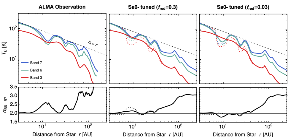
Figure 20.— Same as Figure 12, but for model Sa0-tuned with the modified fragment size distribution given by Equation (33). The center and right panels are for fragment reduction factor $f_{\rm red}=0.3$ (center panels) and 0.03 (right panels).

We now recalculate the radial profiles of $T_{\rm B}$ and $\alpha_{\rm B6\textrm{--}B7}$ for model Sa0-tuned using Equation (33) instead of Equation (20). The results are shown in the center and right panels of Figure 20. These together with the result for $f_{\rm red}=1$ (the center panels in Figure 19) show that both $T_{\rm B}$ and $\alpha_{\rm B6\textrm{--}B7}$ in the two innermost emission dips decrease as $f_{\rm red}$ is decreased. In these inner regions, the radius $a_{*}$ of the largest (mass-dominating) aggregates is significantly larger than millimeters, and therefore the fragments smaller than millimeters have a non-negligible contribution to the millimeter dust opacity. In this case, the opacity index $\beta_{\rm 0.87\textrm{--}1.3~{}mm}$ decreases toward zero, which is the value in the geometric optics limit, as the amount of the fragments decreases (see, e.g., Draine, 2006). This explains why a lower value of $f_{\rm red}$ leads to a lower value of the spectral slope in the optically thin inner dips where the relation $\alpha_{\rm 0.87\textrm{--}1.3~{}mm}\approx\beta_{\rm 0.87\textrm{--}1.3~{}mm}+2$ applies. In the case of $f_{\rm red}=0.03$, the spectral slope in the innermost emission dip falls below two due to the effect of the frequency-dependent angular resolution already mentioned in Section 5.5. We find that the results for $f_{\rm red}=0.3$ and $0.03$ better reproduce the observed depths of the two innermost emission dips than the result for $f_{\rm red}=1$. However, these low-$f_{\rm red}$ models yield poorer agreement with the observed value of $\alpha_{\rm B6\textrm{--}B7}$ in these emission dips. Varying the value of $f_{\rm red}$ within the range $0.03$–1 has no effect on the predictions for $T_{\rm B}$ and $\alpha_{\rm B6\textrm{--}B7}$ outside the two innermost emission dips. Taken together, we cannot judge at this point which value of $f_{\rm red}$ best reproduces the observed appearance of HL Tau. In any case, the effects of assuming lower values of $f_{\rm red}$ are not significant as long as $f_{\rm red}$ is higher than 0.3, the value we expect for unsintered aggregates in the dark rings.

7.3. Evolution of the Monomer Size Distribution and Possible Planetesimal Formation near the ${\rm H_{2}O}$ Sintering Zone

We have assumed that vapor transport within an aggregate, which drives sintering, does not alter the size of monomer grains. In reality, this is not true because the growth of necks must be compensated by the shrinkage of the bodies of monomers. Furthermore, if the monomers within an aggregate are not uniform in size, a small number of large monomers may grow, the phenomenon known as Ostwald ripening (see, e.g., Lifshitz & Pitaevskii 1981), while smaller ones may completely evaporate leaving silicate grains (Sirono, 2011a; Kuroiwa & Sirono, 2011). The evolution of the monomer size distribution is negligible in the sintering zones of minor volatiles like ${\rm NH_{3}}$ and ${\rm CH_{4}}$ (as noted in the introduction, sintering can still occur because the neck volume is much smaller than the monomer volume). However, this is not the case for water ice since it constitutes more than half of the monomer volume.

As pointed out by Kuroiwa & Sirono (2011), the evolution of the monomer size distribution due to water vapor transport would result in a decrease in the sticking efficiency of the icy aggregates. Kuroiwa & Sirono (2011) showed that water vapor transport within an aggregate produces a small number of large ice-rich monomers and a large number of small bare silicate monomers. Aggregates made of the two populations of monomers would be fragile, like sintered aggregates made of equally ice-coated grains, because the total binding energy ($\propto$ number of contacts) of the former would be determined by weak silicate–silicate contacts. These aggregates would experience catastrophic disruption and pile up near the ${\rm H_{2}O}$ snow line in a similar way to sintered aggregates.

In addition, the evaporation of small monomers could directly result in fragmentation of the icy aggregates. Sirono (2011a) demonstrated that an aggregate made of initially submicron-sized ${\rm H_{2}O}$ monomers breaks up into large detached monomers of radii $\sim 1$–10 ${\rm\mu m}$ (see also Kuroiwa & Sirono 2011). This spontaneous breakup would also produce a pileup of dust near the ${\rm H_{2}O}$ snow line, but the surface density contrast provided by this effect that could be much more significant than that by than sintering-induced fragmentation because the micron-sized monomers are much more strongly coupled to the disk gas than aggregates. Sirono (2011a) points out the dust surface density in the ${\rm H_{2}O}$ sintering zone can become high enough to trigger the formation of icy planetesimals via the gravitational instability (Goldreich & Ward, 1973; Sekiya, 1998; Youdin & Shu, 2002).

Thus, the evolution of the monomer size distribution due to vapor transport would further promote the fragmentation and accumulation of aggregates in the ${\rm H_{2}O}$ sintering zone. This may not affect the observational appearance of the HL Tau disk because the ${\rm H_{2}O}$ sintering zone is already optically thick even without the monomer size evolution. However, this could have a significant effect on planet(esimal) formation near the ${\rm H_{2}O}$ snow line.

7.4. Possible Effects of Porosity Evolution

We have neglected the evolution of the porosity of icy aggregates by assuming the fixed aggregate internal density of $0.24~{}{\rm g~{}cm^{-3}}$. In reality, the porosity of aggregates (much smaller than planetesimals) can vary greatly through collisions (e.g., Ormel et al., 2007; Suyama et al., 2008; Okuzumi et al., 2009), compression by gas drag (Kataoka et al., 2013b, a), and condensation and sintering of ${\rm H_{2}O}$ ice (again, minor volatile ices occupy only a small fraction of grain volume and are therefore negligible here). In the absence of the compaction due to condensation and sintering, the internal density of icy aggregates in protoplanetary disks can decline to as low as $10^{-4}$–$10^{-3}~{}{\rm g~{}cm^{-3}}$ (Okuzumi et al., 2012; Kataoka et al., 2013b).

The porosity evolution has two important effects on the evolution of icy aggregates. First, fluffy aggregates tend to grow to the size regime where the gas drag onto the aggregates is determined by Stokes’ law. This particularly occurs in inner regions of protoplanetary disks where the mean free path of the disk gas molecules is short. In the Stokes drag regime, the growth limit given by Equation (30) no longer applies because that limit assumes Epstein’s drag law. Okuzumi et al. (2012) found that fluffy aggregates that are subject to Stokes’ drag law grow fast enough to overcome the radial drift barrier. In a massive protoplanetary disk as considered in this study, icy aggregates break through the drift barrier and form icy planetesimals at $r\lesssim 10~{}{\rm AU}$ (see the bottom right panel of Kataoka et al. 2013a). Second, the millimeter absorption opacity of large porous aggregates is similar to that of small compact aggregates because $\kappa_{\rm d,\nu}$ can be approximated as a function of the product $\rho_{\rm int}a$ (Kataoka et al., 2014).

In this study, all these important effects have been neglected by fixing the aggregate porosity to a relatively low value. Rapid coagulation beyond the Epstein drag regime could strongly reduce the optical depth in the non-sintering zone lying at $r\sim 10~{}{\rm AU}$, where the radial drift barrier determines the maximum size of the relatively compact aggregates that we assumed in this study. This effect should be studied in detail in future work.

On the other hand, the above two effects are less important at $r\gtrsim 10~{}{\rm AU}$, where even the highly fluffy aggregates would grow within the Epstein drag regime. To show this, we first note that neither ${\rm St}_{\rm drift}$ (Equation (30)) nor ${\rm St}_{\rm frag}$ (Equation (32)) depends on $\rho_{\rm int}$ (note again that Epstein’s law is used in the derivation of Equation (30)). This means that porosity evolution has no effect on the maximum attainable Stokes number at each $r$, and therefore does not change the radial distribution of $\Sigma_{\rm d}$ since the radial advection velocity $v_{r}$ is a function of ${\rm St}$ (see Equation (10)). Porosity evolution does not change the dust absorption opacity $\kappa_{\rm d,\nu}$ either since the product $\rho_{\rm int}a_{*}$ is proportional to ${\rm St}$ in the Epstein regime (see Equation (9)). This is a natural consequence of the fact that both the stopping time in the Epstein regime and the absorption opacity are determined by the mass-to-area ratio $m/\pi a^{2}(\sim\rho_{\rm int}a)$ of the aggregates. Taken together, the radial distribution of the absorption optical depth $\tau_{\nu}\propto\kappa_{\rm d,\nu}\Sigma_{\rm d}$ is independent of the aggregate porosity as long as the aggregates grow within the Epstein drag regime.

Nevertheless, porosity evolution might have some important observational consequence in the outer disk region. The millimeter continuum emission from the HL Tau disk is known to be polarized in the direction roughly perpendicular to the disk major axis at a level of 0.9% in the average degree of polarization (Stephens et al., 2014). Yang et al. (2015) and Kataoka et al. (2015b) point out that self-scattering of thermal emission by dust rings (Kataoka et al., 2015a) can explain the polarization observation. However, this mechanism produces a degree of polarization of $\approx 1\%$ only when the size of the dust particles falls within a particular range. For example, if the particles are compact and their size distribution obeys our Equation (20), the self-scattering scenario is consistent with the observation only when the maximum particle size $a_{\rm max}$ ($=a_{*}$ in this study) is $\sim 0.1~{}{\rm mm}$ (Yang et al., 2015; Kataoka et al., 2015b), which is considerably smaller than the size of mass-dominating aggregates predicted in this study. In the compact particle model, a particle size larger than a millimeter is ruled out because the scattered emission would then be too weakly polarized (see also Kataoka et al., 2015a). By contrast, large but fluffy aggregates are known to produce a highly polarization scattered light like constituent monomers do (Min et al., 2016), and therefore might be able to explain the polarization observation of HL Tau.

7.5. Possible Effects of Condensation Growth

We have neglected the condensation growth of ice particles near the snow lines. In fact, a recent study by Ros & Johansen (2013) has shown that condensation growth can be effective at locations slightly outside the ${\rm H_{2}O}$ snow line. This effect might change our predictions for dust evolution near ${\rm H_{2}O}$ snow line, because condensation dominantly takes place on the smallest particles, i.e., monomers. If condensation dominates over sintering-induced fragmentation and bouncing, the regions slightly outside the snow lines would be seen as ${\it dark}$ rings at millimeter wavelengths as already pointed out by Zhang et al. (2015). However, it is unclear whether condensation growth becomes important for volatiles less abundant than ${\rm H_{2}O}$, like ${\rm CO}$ and ${\rm NH_{3}}$. To address this open question, we will incorporate condensation growth into our global dust evolution simulations in future work.

7.6. Sintering-induced Ring Formation in Other Objects?

Perhaps the strongest prediction from our model, as well as from the model of Zhang et al. (2015), is that the multiple dust rings may not be peculiar to the HL Tau disk. In principle, sintering-induced ring formation operates as long as the disk is not too depleted of dust (or not too old), the monomers are sufficiently small to cause rapid sintering, and turbulence is strong enough to cause disruption of sintered aggregates. If these conditions are satisfied, axisymmetric dust rings emerge slightly outside the snow lines of relatively major volatiles. An intriguing object in this context is TW Hya. For this system, the CO snow line has been indirectly detected at an orbital distance of $\sim 30$ AU (Qi et al., 2013), and furthermore, near-infrared scattered light images of the disk suggest the presence of two axisymmetric dust gaps at $\sim 80$ AU (Debes et al., 2013) and $\sim 20$ AU (Akiyama et al., 2015; Rapson et al., 2015). A latest ALMA observation has shown that there is also a gap in millimeter dust emission in the vicinity of the 20 AU scattered light gap (Nomura et al., 2015). The gaps at 80 AU and 20 AU could be associated with non-sintering zones exterior to and interior to the CO sintering zone, respectively. However, it is not obvious whether our ring formation mechanism directly applies to TW Hya because this object is known to be much older than HL Tau (at least 3 Myr; Vacca & Sandell 2011). This question should also be addressed in future work.

8. Conclusions

Motivated by the recent ALMA observations of the HL Tau disk, we have explored the possibility that sintering of icy dust aggregates might lead to the formation of multiple dust rings in a protoplanetary disk. Sintering is a particle fusion process that occurs when the temperature is slightly below the melting point. Sintered aggregates are generally harder but less sticky than unsintered aggregates. Therefore, if dust aggregates in a protoplanetary disk consist of various materials, their growth can be suppressed at different orbits corresponding to the sublimation fronts of different materials. This possibility was originally pointed out by Sirono (1999, 2011b), and here we have for the first time studied its effects on the global evolution of dust in a protoplanetary disk.

Following Sirono (2011b), we have regard aggregates as sintered if their sintering timescale is shorter than their collision timescale (Section 3.4). This criterion defines the “sintering zones” in which one of the volatile species included in the aggregates causes sintering. The temperature profile of the HL Tau disk has been modeled based on the millimeter intensity maps provided by the ALMA observations (ALMA Partnership et al., 2015) together with the assumption that the central emission peak and inner bright rings are optically thick at 1 mm (Section 2.1, Figure 1). Based on the aggregate collision simulations by Sirono & Ueno (2014), we have assumed that sintered aggregates have a maximum sticking velocity that is 60% lower than that for unsintered aggregates (Equations (18) and (19); Figure 5(a)). For both sintered and unsintered aggregates, we have regarded collisions at velocities higher than the threshold disruptive (Equation (15); Figure 5(b)).

Using the aggregate sintering model described above, we have simulated the global evolution of dust in the HL Tau disk for various sets of model parameters. As a first step toward more comprehensive modeling, we focused on the evolution of mass-dominating (largest) aggregates, and assumed a power-law size distribution for smaller aggregates when we convert the simulation data into radial profiles of millimeter dust emission. Key parameters in our model are the strength of turbulence ($\alpha_{\rm t}$), the size of monomers that constitute the aggregates ($a_{0}$), and the sublimation energies of the volatiles ($L_{j}$). The monomer size is relevant here because it controls the timescale of sintering (Equation (6)) and the fragmentation strength of dust aggregates (Equations (18) and (19)).

Our key findings are summarized as follows.

1. Because dust is gradually lost to the central star owing to radial drift, the total dust mass in the disk decreases with time (Section 5.1). For the total disk mass of $0.2~{}M_{\sun}$ and the initial dust-to-gas mass ratio of 0.01, our HL Tau disk models best reproduce the millimeter flux densities from the ALMA observations when the disk age in the models is chosen to be 0.1–0.5 Myr. This is consistent with the general belief that HL Tau is a young ($\lesssim$ 1 Myr) protoplanetary disk.

2. Dust aggregates pile up in the sintering zones due to the combined effect of radial drift and sintering-induced fragmentation (Section 5.2). In general, aggregates grow locally until either rapid radial drift or fragmentation starts to halt their growth. After that, the aggregates start to drift toward the central star at a velocity proportional to the maximum size. Sintered aggregates have a lower maximum size and hence a lower inward drift velocity than unsintered aggregates simply because the former tend to disrupt more easily upon collision. For this reason, aggregates tend to pile up in the sintering zones.

3. At millimeter wavelengths, the sintering zones are seen as bright rings because the dust surface density in the sintering zones is higher than in the non-sintering zones (Section 5.4). In particular, at the wavelengths of 0.87 mm and 1.3 mm, the three innermost sintering zones (which correspond to ${\rm H_{2}O}$, ${\rm NH_{3}}$–${\rm CO_{2}}$–${\rm H_{2}S}$, and ${\rm C_{2}H_{6}}$, respectively) are optically thick, producing a millimeter spectral index of $\approx 2$. The predicted spectral index and brightness temperatures are consistent with those of the central emission peak and two innermost bright rings of the HL Tau disk (Section 5.5). Our model also predicts an optically thin emission peak at $\approx 80$ AU, which is associated with the ${\rm CH_{4}}$ sintering zone, and two optically thin dark rings of a spectral slope of 2.3–2.5 at $\lesssim 40~{}{\rm AU}$, which are associated with the two innermost non-sintering zones. These are all consistent with the ALMA observation.

4. The sintering-induced ring patterns diminish as the disk becomes depleted of dust (Section 5.3). As the dust-to-gas mass ratio decreases, aggregates collide with each other less frequently, making their maximum size more severely limited by radial drift rather than fragmentation. The sintering-induced rings disappear once radial drift dominates over fragmentation even in the sintering zones. For a disk having the total mass of $0.2~{}M_{\sun}$, the characteristic radius of 150 AU, and the initial dust-to-gas mass ratio of 0.01, we find that the sintering-induced rings decay in 2 Myr. The ring patterns of HL Tau might be a sign of its youth.

5. Models that assume lower turbulence parameter $\alpha_{\rm t}$ toward the central star best reproduce the multiple ring structure of HL Tau (Section 6.2). If $\alpha_{\rm t}$ were radially constant, turbulence-driven collision velocity $\propto\sqrt{\alpha_{\rm t}T}$ would increase with decreasing radial distance $r$. In this case, either unsintered aggregates would fragment at small $r$, or sintered aggregates would fragment at large $r$. The former case does not reproduce dark rings at small $r$, while the latter case does not reproduce bright rings at large $r$. The radial dependence of $\alpha_{\rm t}$ suggested by our model is qualitatively consistent with the predictions from magnetohydrodynamical turbulence models.

6. The vertical extent the observed dust rings places a strong constraint on the turbulence strength and monomer size assumed in our model (Section 6.3). When $a_{0}\gg 1~{}\micron$, sintering would be too slow to induce dust ring formation. When $a_{0}\ll 1~{}\micron$, disruption of sintered aggregates would require turbulence that is too strong to allow dust settling to the midplane. If the macroscopic dust particles in the HL Tau disk must already have settled as suggested by previous studies (Kwon et al., 2011; Pinte et al., 2016), disk turbulence must be moderately weak ($10^{-4}<\alpha_{\rm t}\lesssim 10^{-3}$) and monomers must be micron-sized ($1~{}\micron\lesssim a_{0}<4~{}\micron$). The predicted monomer size might be consistent with the near-infrared observations of HL Tau that suggesting the presence of micron-sized grains on the surface of its circumstellar envelope (Lucas et al., 2004; Murakawa et al., 2008).

7. The exact locations and widths of the dust rings predicted by our model are subject to uncertainties in the vapor pressure data (Section 6.4). In general, a 10% uncertainty in the sublimation energy of a volatile species causes a $\sim 20\%$ uncertainty in the predicted location of the volatile’s sintering zone. We find that reducing the sublimation energies of ${\rm H_{2}O}$, ${\rm NH_{3}}$, and ${\rm C_{2}H_{6}}$ by only 10% from our fiducial values significantly improves our predictions for the observational appearance of the ring structures in an inner region of the HL Tau disk. The models using the tuned sublimation energies reproduce the radial positions of the HL Tau’s inner rings to an accuracy of $\lesssim 30\%$.

References

- Adachi et al. (1976) Adachi, I., Hayashi, C., & Nakazawa, K. 1976, Progress of Theoretical Physics, 56, 1756
- Akiyama et al. (2015) Akiyama, E., Muto, T., Kusakabe, N., et al. 2015, ApJ, 802, L17
- ALMA Partnership et al. (2015) ALMA Partnership, Brogan, C. L., Pérez, L. M., et al. 2015, ApJ, 808, L3
- Andrews et al. (2009) Andrews, S. M., Wilner, D. J., Hughes, A. M., Qi, C., & Dullemond, C. P. 2009, ApJ, 700, 1502
- Bai (2011) Bai, X.-N. 2011, ApJ, 739, 50
- Balbus & Hawley (1991) Balbus, S. A., & Hawley, J. F. 1991, ApJ, 376, 214
- Bauer et al. (1997) Bauer, I., Finocchi, F., Duschl, W. J., Gail, H.-P., & Schloeder, J. P. 1997, A&A, 317, 273
- Beckwith et al. (1990) Beckwith, S. V. W., Sargent, A. I., Chini, R. S., & Guesten, R. 1990, AJ, 99, 924
- Birnstiel et al. (2010) Birnstiel, T., Dullemond, C. P., & Brauer, F. 2010, A&A, 513, A79
- Birnstiel et al. (2012) Birnstiel, T., Klahr, H., & Ercolano, B. 2012, A&A, 539, A148
- Birnstiel et al. (2011) Birnstiel, T., Ormel, C. W., & Dullemond, C. P. 2011, A&A, 525, A11
- Blackford (2007) Blackford, J. R. 2007, Journal of Physics D Applied Physics, 40, 355
- Brauer et al. (2008) Brauer, F., Dullemond, C. P., & Henning, T. 2008, A&A, 480, 859
- Chokshi et al. (1993) Chokshi, A., Tielens, A. G. G. M., & Hollenbach, D. 1993, ApJ, 407, 806
- Collings et al. (2004) Collings, M. P., Anderson, M. A., Chen, R., et al. 2004, MNRAS, 354, 1133
- Collings et al. (2003) Collings, M. P., Dever, J. W., Fraser, H. J., McCoustra, M. R. S., & Williams, D. A. 2003, ApJ, 583, 1058
- Debes et al. (2013) Debes, J. H., Jang-Condell, H., Weinberger, A. J., Roberge, A., & Schneider, G. 2013, ApJ, 771, 45
- Dipierro et al. (2015) Dipierro, G., Price, D., Laibe, G., et al. 2015, MNRAS, 453, L73
- Dohnanyi (1969) Dohnanyi, J. S. 1969, J. Geophys. Res., 74, 2531
- Dominik & Tielens (1997) Dominik, C., & Tielens, A. G. G. M. 1997, ApJ, 480, 647
- Dong et al. (2015) Dong, R., Zhu, Z., & Whitney, B. 2015, ApJ, 809, 93
- Draine (2003) Draine, B. T. 2003, ApJ, 598, 1026
- Draine (2006) —. 2006, ApJ, 636, 1114
- Dubrulle et al. (1995) Dubrulle, B., Morfill, G., & Sterzik, M. 1995, Icarus, 114, 237
- Dzyurkevich et al. (2010) Dzyurkevich, N., Flock, M., Turner, N. J., Klahr, H., & Henning, T. 2010, A&A, 515, A70
- Estrada et al. (2016) Estrada, P. R., Cuzzi, J. N., & Morgan, D. A. 2016, ApJ, in press, arXiv:1506.01420
- Ferrier (1994) Ferrier, B. S. 1994, Journal of the Atmospheric Sciences, 51, 249
- Flock et al. (2015) Flock, M., Ruge, J. P., Dzyurkevich, N., et al. 2015, A&A, 574, A68
- Fouchet et al. (2010) Fouchet, L., Gonzalez, J.-F., & Maddison, S. T. 2010, A&A, 518, A16
- Garaud (2007) Garaud, P. 2007, ApJ, 671, 2091
- Goldreich & Ward (1973) Goldreich, P., & Ward, W. R. 1973, ApJ, 183, 1051
- Gonzalez et al. (2015) Gonzalez, J.-F., Laibe, G., Maddison, S. T., Pinte, C., & Ménard, F. 2015, MNRAS, 454, L36
- Gonzalez et al. (2012) Gonzalez, J.-F., Pinte, C., Maddison, S. T., Ménard, F., & Fouchet, L. 2012, A&A, 547, A58
- Guilloteau et al. (2011) Guilloteau, S., Dutrey, A., Piétu, V., & Boehler, Y. 2011, A&A, 529, A105
- Hartmann et al. (1998) Hartmann, L., Calvet, N., Gullbring, E., & D’Alessio, P. 1998, ApJ, 495, 385
- Hayashi et al. (1993) Hayashi, M., Ohashi, N., & Miyama, S. M. 1993, ApJ, 418, L71
- Haynes (2014) Haynes, W. M. 2014, CRC Handbook of Chemistry and Physics, 95th edn. (Boca Raton, FL: CRC press)
- Johansen et al. (2009) Johansen, A., Youdin, A., & Klahr, H. 2009, ApJ, 697, 1269
- Johnson et al. (1971) Johnson, K. L., Kendall, K., & Roberts, A. D. 1971, Royal Society of London Proceedings Series A, 324, 301
- Kanagawa et al. (2015) Kanagawa, K. D., Muto, T., Tanaka, H., et al. 2015, ApJ, 806, L15
- Kataoka et al. (2015a) Kataoka, A., Muto, T., Momose, M., Tsukagoshi, T., & Dullemond, C. P. 2015a, ArXiv e-prints, arXiv:1507.08902
- Kataoka et al. (2014) Kataoka, A., Okuzumi, S., Tanaka, H., & Nomura, H. 2014, A&A, 568, A42
- Kataoka et al. (2013a) Kataoka, A., Tanaka, H., Okuzumi, S., & Wada, K. 2013a, A&A, 557, L4
- Kataoka et al. (2013b) —. 2013b, A&A, 554, A4
- Kataoka et al. (2015b) Kataoka, A., Muto, T., Momose, M., et al. 2015b, ApJ, 809, 78
- Kitamura et al. (2002) Kitamura, Y., Momose, M., Yokogawa, S., et al. 2002, ApJ, 581, 357
- Kornet et al. (2001) Kornet, K., Stepinski, T. F., & Różyczka, M. 2001, A&A, 378, 180
- Kretke & Lin (2007) Kretke, K. A., & Lin, D. N. C. 2007, ApJ, 664, L55
- Krijt et al. (2015) Krijt, S., Ormel, C. W., Dominik, C., & Tielens, A. G. G. M. 2015, A&A, 574, A83
- Krijt et al. (2016) —. 2016, A&A, 586, A20
- Kuroiwa & Sirono (2011) Kuroiwa, T., & Sirono, S.-i. 2011, ApJ, 739, 18
- Kwon et al. (2011) Kwon, W., Looney, L. W., & Mundy, L. G. 2011, ApJ, 741, 3
- Kwon et al. (2015) Kwon, W., Looney, L. W., Mundy, L. G., & Welch, W. J. 2015, ApJ, 808, 102
- Laibe (2014) Laibe, G. 2014, MNRAS, 437, 3037
- Lambrechts & Johansen (2014) Lambrechts, M., & Johansen, A. 2014, A&A, 572, A107
- Lifshitz & Pitaevskii (1981) Lifshitz, E. M., & Pitaevskii, L. P. 1981, Physical Kinetics (Oxford: Pergamon)
- Lorén-Aguilar & Bate (2015) Lorén-Aguilar, P., & Bate, M. R. 2015, MNRAS, 453, L78
- Lucas et al. (2004) Lucas, P. W., Fukagawa, M., Tamura, M., et al. 2004, MNRAS, 352, 1347
- Luna et al. (2014) Luna, R., Satorre, M. Á., Santonja, C., & Domingo, M. 2014, A&A, 566, A27
- Martín-Doménech et al. (2014) Martín-Doménech, R., Muñoz Caro, G. M., Bueno, J., & Goesmann, F. 2014, A&A, 564, A8
- Mathis et al. (1977) Mathis, J. S., Rumpl, W., & Nordsieck, K. H. 1977, ApJ, 217, 425
- Men’shchikov et al. (1999) Men’shchikov, A. B., Henning, T., & Fischer, O. 1999, ApJ, 519, 257
- Meyer (1977) Meyer, B. 1977, Sulfur, energy, and environment (Elsevier Scientific Pub. Co.)
- Min et al. (2016) Min, M., Rab, C., Woitke, P., Dominik, C., & Ménard, F. 2016, A&A, 585, A13
- Moses et al. (1992) Moses, J. I., Allen, M., & Yung, Y. L. 1992, Icarus, 99, 318
- Mumma & Charnley (2011) Mumma, M. J., & Charnley, S. B. 2011, ARA&A, 49, 471
- Mundt et al. (1988) Mundt, R., Buehrke, T., & Ray, T. P. 1988, ApJ, 333, L69
- Murakawa et al. (2008) Murakawa, K., Oya, S., Pyo, T.-S., & Ishii, M. 2008, A&A, 492, 731
- Nomura et al. (2015) Nomura, H., Tsukagoshi, T., Kawabe, R., et al. 2015, ArXiv e-prints, arXiv:1512.05440
- Okuzumi & Hirose (2012) Okuzumi, S., & Hirose, S. 2012, ApJ, 753, L8
- Okuzumi et al. (2012) Okuzumi, S., Tanaka, H., Kobayashi, H., & Wada, K. 2012, ApJ, 752, 106
- Okuzumi et al. (2009) Okuzumi, S., Tanaka, H., & Sakagami, M.-a. 2009, ApJ, 707, 1247
- Ormel (2014) Ormel, C. W. 2014, ApJ, 789, L18
- Ormel & Cuzzi (2007) Ormel, C. W., & Cuzzi, J. N. 2007, A&A, 466, 413
- Ormel et al. (2007) Ormel, C. W., Spaans, M., & Tielens, A. G. G. M. 2007, A&A, 461, 215
- Paardekooper & Mellema (2004) Paardekooper, S.-J., & Mellema, G. 2004, A&A, 425, L9
- Paardekooper & Mellema (2006) —. 2006, A&A, 453, 1129
- Pinilla et al. (2012) Pinilla, P., Benisty, M., & Birnstiel, T. 2012, A&A, 545, A81
- Pinte et al. (2016) Pinte, C., Dent, W. R. F., Ménard, F., et al. 2016, ApJ, 816, 25
- Pollack et al. (1994) Pollack, J. B., Hollenbach, D., Beckwith, S., et al. 1994, ApJ, 421, 615
- Poppe (2003) Poppe, T. 2003, Icarus, 164, 139
- Qi et al. (2013) Qi, C., Öberg, K. I., Wilner, D. J., et al. 2013, Science, 341, 630
- Rapson et al. (2015) Rapson, V. A., Kastner, J. H., Millar-Blanchaer, M. A., & Dong, R. 2015, ApJ, 815, L26
- Rietmeijer (1993) Rietmeijer, F. J. M. 1993, Earth and Planetary Science Letters, 117, 609
- Ros & Johansen (2013) Ros, K., & Johansen, A. 2013, A&A, 552, A137
- Saito & Sirono (2011) Saito, E., & Sirono, S.-i. 2011, ApJ, 728, 20
- Sano et al. (2000) Sano, T., Miyama, S. M., Umebayashi, T., & Nakano, T. 2000, ApJ, 543, 486
- Sargent & Beckwith (1991) Sargent, A. I., & Beckwith, S. V. W. 1991, ApJ, 382, L31
- Sato et al. (2016) Sato, T., Okuzumi, S., & Ida, S. 2016, A&A, in press, arXiv:1512.02414
- Seizinger et al. (2013) Seizinger, A., Krijt, S., & Kley, W. 2013, A&A, 560, A45
- Sekiya (1998) Sekiya, M. 1998, Icarus, 133, 298
- Sirono (1999) Sirono, S. 1999, A&A, 347, 720
- Sirono (2011a) Sirono, S.-i. 2011a, ApJ, 733, L41
- Sirono (2011b) —. 2011b, ApJ, 735, 131
- Sirono & Ueno (2014) Sirono, S.-i., & Ueno, H. 2014, in COSPAR Meeting, Vol. 40, 40th COSPAR Scientific Assembly, 3110
- Stephens et al. (2014) Stephens, I. W., Looney, L. W., Kwon, W., et al. 2014, Nature, 514, 597
- Suyama et al. (2008) Suyama, T., Wada, K., & Tanaka, H. 2008, ApJ, 684, 1310
- Swinkels & Ashby (1981) Swinkels, F., & Ashby, M. 1981, Acta Metallurgica, 29, 259
- Takahashi & Inutsuka (2014) Takahashi, S. Z., & Inutsuka, S.-i. 2014, ApJ, 794, 55
- Takeuchi & Lin (2005) Takeuchi, T., & Lin, D. N. C. 2005, ApJ, 623, 482
- Tanaka et al. (1996) Tanaka, H., Inaba, S., & Nakazawa, K. 1996, Icarus, 123, 450
- Uribe et al. (2011) Uribe, A. L., Klahr, H., Flock, M., & Henning, T. 2011, ApJ, 736, 85
- Vacca & Sandell (2011) Vacca, W. D., & Sandell, G. 2011, ApJ, 732, 8
- Wada et al. (2013) Wada, K., Tanaka, H., Okuzumi, S., et al. 2013, A&A, 559, A62
- Wada et al. (2008) Wada, K., Tanaka, H., Suyama, T., Kimura, H., & Yamamoto, T. 2008, ApJ, 677, 1296
- Wada et al. (2009) —. 2009, ApJ, 702, 1490
- Warren (1984) Warren, S. G. 1984, Appl. Opt., 23, 1206
- Weidenschilling (1977) Weidenschilling, S. J. 1977, MNRAS, 180, 57
- Whipple (1972) Whipple, F. L. 1972, in From Plasma to Planet, ed. A. Elvius, 211
- White & Hillenbrand (2004) White, R. J., & Hillenbrand, L. A. 2004, ApJ, 616, 998
- Yamamoto et al. (1983) Yamamoto, T., Nakagawa, N., & Fukui, Y. 1983, A&A, 122, 171
- Yang et al. (2015) Yang, H., Li, Z.-Y., Looney, L., & Stephens, I. 2015, MNRAS, in press, arXiv:1507.08353
- Youdin (2011) Youdin, A. N. 2011, ApJ, 731, 99
- Youdin & Lithwick (2007) Youdin, A. N., & Lithwick, Y. 2007, Icarus, 192, 588
- Youdin & Shu (2002) Youdin, A. N., & Shu, F. H. 2002, ApJ, 580, 494
- Zhang et al. (2015) Zhang, K., Blake, G. A., & Bergin, E. A. 2015, ApJ, 806, L7
- Zhu et al. (2012) Zhu, Z., Nelson, R. P., Dong, R., Espaillat, C., & Hartmann, L. 2012, ApJ, 755, 6
- Zubko et al. (1996) Zubko, V. G., Mennella, V., Colangeli, L., & Bussoletti, E. 1996, MNRAS, 282, 1321