Comparing models of the periodic variations in spin-down and beam-width for PSR B1828-11

Abstract

We build a framework using tools from Bayesian data analysis to evaluate models explaining the periodic variations in spin-down and beam-width of PSR B1828-11. The available data consists of the time averaged spin-down rate, which displays a distinctive double-peaked modulation, and measurements of the beam-width. Two concepts exist in the literature that are capable of explaining these variations; we formulate predictive models from these and quantitatively compare them. The first concept is phenomenological and stipulates that the magnetosphere undergoes periodic switching between two meta-stable states as first suggested by Lyne et al.. The second concept, precession, was first considered as a candidate for the modulation of B1828-11 by Stairs et al.. We quantitatively compare models built from these concepts using a Bayesian odds-ratio. Because the phenomenological switching model itself was informed by this data in the first place, it is difficult to specify appropriate parameter-space priors that can be trusted for an unbiased model comparison. Therefore we first perform a parameter estimation using the spin-down data, and then use the resulting posterior distributions as priors for model comparison on the beam-width data. We find that a precession model with a simple circular Gaussian beam geometry fails to appropriately describe the data, while allowing for a more general beam geometry provides a good fit to the data. The resulting odds between the precession model (with a general beam geometry) and the switching model are estimated as $10^{2.7\pm 0.5}$ in favour of the precession model.

1 Introduction

The pulsar B1828-11 demonstrates periodic variability in its pulse timing and beam shape at harmonically related periods of 250, 500, and 1000 days. The modulations in the timing was first taken as evidence that the pulsar is orbited by a system of planets by Bailes et al. (1993). A more complete analysis by Stairs et al. (2000) concluded that the corresponding changes in the beam-shape would require at least two of the planets to interact with the magnetosphere, which does not seem credible. Instead the authors proposed that the correlation between timing data and beam-shape suggested the pulsar was undergoing free precession. If true, such a claim would require rethinking of the vortex-pinning model used to explain the pulsar glitches since the pinning should lead to much shorter modulation period than observed (Shaham, 1977), and fast damping of the modulation (Link, 2003).

The idea of precession for B1828-11 has been studied extensively in the literature: Jones & Andersson (2001) derived the observable modulations due to precession and noted that the electromagnetic spin-down torque will amplify these modulations. Link & Epstein (2001) fitted a torqued-precession model to the spin-down and beam-shape followed by Akgün et al. (2006) where a variety of shapes and the form of the spin-down torque were tested. All of these authors agree that precession is a credible candidate to explain the observed periodic variations: furthermore to explain the double-peaked spin-down modulations, the so-called wobble angle must be small while the magnetic dipole must be close to $\uppi/2$.

More recently Arzamasskiy et al. (2015) updated the previous estimates (based on a vacuum approximation) to a plasma filled magnetosphere. They also find that the magnetic dipole and spin-vector must be close to orthogonal, but solutions could exist where it is the wobble angle which is close to $\uppi/2$ while the magnetic dipole lies close to the angular momentum vector; we will not consider such a model here, but note it is a valid alternative which deserves testing.

The distinctive spin-down of B1828-11 was analysed by Seymour & Lorimer (2013) for evidence of chaotic behaviour. They found evidence that B1828-11 was subject to three dynamic equations with the spin-down rate being one governing variable. This further motivates the precession model since it results from applying Euler’s three rigid body equations to a non-spherical body (Landau & Lifshitz, 1969).

The precession hypothesis was challenged by Lyne et al. (2010) when reanalysing the data. They noted that in order to measure the spin-down and beam-shape with any accuracy required time averaging over periods $\sim 100$ days, smoothing out any behaviour acting on this time-scale. Motivated by the intermittent pulsar B1931+24, they put forward the phenomenological hypothesis that instead the magnetosphere is undergoing periodic switching between (at least) two metastable states. Such switching would result in correlated changes in the beam-width and spin-down rate. They returned to the data and instead of studying a time-averaged beam-shape-parameter as done by Stairs et al. (2000), they instead considered the beam-width at 10% of the observed maximum $W_{10}$. This quantity is time-averaged, but only for each observation lasting $\sim 1$hr. This makes $W_{10}$ insensitive to any changes which occur on time-scales shorter than an hour. If the meta-stable states last longer than this, $W_{10}$ will be able to resolve the switching. The relevant data was kindly supplied to us courtesy of Lyne et al. (2010), and is reproduced in Fig. 1. From these observations, Lyne et al. (2010) concluded that the individual measurements of $W_{10}$ for B1828-11 did in fact appear to switch between distinct high and low values, as opposed to a smooth modulation between the values, with this switching coinciding with the periodic changes in the spin-down. On this basis, they interpret the modulations of B1828-11 as evidence it is undergoing periodic switching between two magnetospheric states. When studying another pulsar which also displays double-peaked spin-down modulations, Perera et al. (2015) extended the switching model, as discussed in Sec. 3.2, to be capable of producing the double-peak spin-down rate; it is this modification of the switching model which we will be comparing with precession.

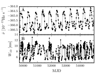
Figure 1: Observed data for PSR B1828-11 spanning from MJD 49710 to MJD 54980. In panel A we reproduce the spin-down rate with error-bars and in panel B the beam-width $W_{10}$ (for which no error bars were available). All data courtesy of Lyne et al. (2010).

In our view, it is not immediately clear by eye whether the data presented in Fig. 1 is sufficient to rule out or even favour either of the precession or switching interpretations. For this reason, in this work we develop a framework in which to evaluate models built from these concepts and argue their merits quantitatively using a Bayesian model comparison. We note that a distinction must be made between a conceptual idea, such as precession, and a particular predictive model built from it. As we will see, each concept can generate multiple models, and furthermore we could imagine using a combination of precession and switching, with the precession acting as the ‘clock’ that modulates the probability of the magnetosphere being in one state or the other, an idea developed by Jones (2012). The models considered here cover the precession and switching interpretations, but we do not claim the models to be the ‘best’ that these hypotheses could produce.

The rest of the work is organised as follows: in Sec. 2 we will describe the framework to fit and evaluate a given model, in Sec. 3 we will define and fit several predictive models from the conceptual ideas, and then in Sec. 4 we shall tabulate the results of the model comparison. Finally, the results are discussed in Sec. 5.

2 Bayesian Methodology

We now introduce a general methodology to compare and evaluate models for this form of data. The technique is well practised in this and other fields and so in this section we intend only to give a brief overview; for a more complete introduction to this subject see Jaynes (2003); Gelman et al. (2013); Sivia & Skilling (1996).

2.1 The odds-ratio and posterior probabilities

There are two issues that we wish to address. Firstly, given two models, how can one say which is preferred, and by what margin? Secondly, assuming a given model, what can be said of the probability distribution of the parameters that appear in that model?

We can address the first issue by making use of Bayes theorem for the probability of model $\mathcal{M}_{i}$ given some data:

$$P(\mathcal{M}_{i}|\textrm{data})=P(\textrm{data}|\mathcal{M}_{i})\frac{P(\mathcal{M}_{i})}{P(\textrm{data})}.$$ (1)

The quantity $P(\textrm{data}|\mathcal{M}_{i})$ in known as the marginal likelihood of model $\mathcal{M}_{i}$ given the data.

In general we cannot compute the probability given in equation (1) because we do not have an exhaustive set of models to calculate $P(\textrm{data})$. However, we can compare two models, say $A$ and $B$, by calculation of their odds-ratio:

$$\mathcal{O}=\frac{P(\mathcal{M}_{A}|\textrm{data})}{P\mathcal{M}_{B}|(\textrm{data})}=\frac{P(\textrm{data}|\mathcal{M}_{A})}{P(\textrm{data}|\mathcal{M}_{B})}\frac{P(\mathcal{M}_{A})}{P(\mathcal{M}_{B})}.$$ (2)

In the rightmost expression, the first factor is the ratio of the marginal likelihoods (also known as the Bayes factor) which we will discuss shortly, while the final factor reflects our prior belief in the two models. If no strong preference exists for one over the other, we may take a non-informative approach and set this equal to unity. We will follow this approach in what follows below.

We need to find a way of computing the marginal likelihoods, $P(\textrm{data}|\mathcal{M}_{i})$. To this end, consider a single model $\mathcal{M}_{i}$ with model parameters $\boldsymbol{\theta}$, and define $P(\textrm{data}|\boldsymbol{\theta},\mathcal{M}_{i})$ as the likelihood function and $P(\boldsymbol{\theta}|\mathcal{M}_{i})$ as the prior distribution for the model parameters. We can then perform the necessary calculations by making use of

$$P(\textrm{data}|\mathcal{M}_{i})=\int P(\textrm{data}|\boldsymbol{\theta},\mathcal{M}_{i})P(\boldsymbol{\theta}|\mathcal{M}_{i})d\boldsymbol{\theta}.$$ (3)

The likelihood function can also be used to explore the second issue of interest, by calculating the joint-probability distribution for the model parameters, also known as the posterior probability distribution:

$$P(\boldsymbol{\theta}|\textrm{data},\mathcal{M}_{i})=\frac{P(\textrm{data}|\boldsymbol{\theta},\mathcal{M}_{i})P(\boldsymbol{\theta}|\mathcal{M}_{i})}{P(\textrm{data}|\mathcal{M}_{i})}.$$ (4)

Note that the marginal likelihood $P(\textrm{data}|\mathcal{M}_{i})$ described above plays the role of a normalising factor in this equation.

In general the integrand of Eqn. (3) makes analytic, or even simple numeric integration difficult or impossible. This is the case for the probability model that we will use and so instead we must turn to sophisticated numerical methods. For this study we use Markov-Chain Monte-Carlo (MCMC) techniques which simulate the joint-posterior distribution for the model parameters up to the normalising constant

$$P(\boldsymbol{\theta}|\textrm{data},\mathcal{M}_{i})\propto P(\textrm{data}|\boldsymbol{\theta},\mathcal{M}_{i})P(\boldsymbol{\theta}|\mathcal{M}_{i}).$$ (5)

In particular we will use the Foreman-Mackey et al. (2013) implementation of the affine-invariant MCMC sampler (Goodman & Weare, 2010) to approximate the posterior density of the model parameters. Further details of our MCMC calculations can be found in appendix A.

Once we are satisfied that we have a good approximation for the joint-posterior density of the model parameters we discuss how to recover the normalising constant to calculate the odds-ratio in Sec. 4.

2.2 Signals in noise

We now need to build a statistical model to relate physical models for the spin-down and beam-width to the data observed in Fig. 1. To do this we will turn to a method widely used to search for deterministic signals in noise.

We assume our observed data $y^{\textrm{obs}}$ is a sum of a stationary zero-mean Gaussian noise process $n(t,\sigma)$ (here $\sigma$ is the standard deviation of the noise process) and a signal model $f(t|\mathcal{M}_{j},\boldsymbol{\theta})$ (where $\boldsymbol{\theta}$ is a vector of the model parameters) such that

$$y^{\textrm{obs}}(t_{i}|\mathcal{M}_{j},\boldsymbol{\theta},\sigma)=f(t_{i}|\mathcal{M}_{j},\boldsymbol{\theta})+n(t_{i},\sigma).$$ (6)

Given a particular signal model, subtracting the model from the data should, if the model and model parameters are correct, leave behind a Gaussian distributed residual - the noise. That is

$$y^{\textrm{obs}}(t_{i}|\mathcal{M}_{j},\boldsymbol{\theta},\sigma)-f(t_{i}|\mathcal{M}_{j},\boldsymbol{\theta})\sim N(0,\sigma).$$ (7)

The data, for either the spin-down or beam-width, consists of $N$ observations $(y^{\textrm{obs}}_{i},t_{i})$. For a single one of these observations, the probability distribution given the model and model parameters is

$$P(y_{i}^{\textrm{obs}}|\mathcal{M}_{j},\boldsymbol{\theta},\sigma)=\frac{1}{\sigma\sqrt{2\uppi}}\exp\left\{\frac{-\left(f(t_{i}|\mathcal{M}_{j},\boldsymbol{\theta})-y_{i}\right)^{2}}{2\sigma^{2}}\right\}.$$ (8)

The likelihood is the product of the $N$ probabilities

$$P(\mathbf{y}^{\mathrm{obs}}|\mathcal{M}_{j},\boldsymbol{\theta},\sigma)=\prod_{i=1}^{N}P(y_{i}^{\textrm{obs}}|\mathcal{M}_{j},\boldsymbol{\theta},\sigma),$$ (9)

where $\mathbf{y}^{\mathrm{obs}}$ denotes the vector of all the observed data.

In Sec. 3 we will define the physical models, $f(t|\mathcal{M}_{j},\boldsymbol{\theta})$, for the precession and switching interpretations; for now we recognise that once defined, we may calculate the likelihood of the data under the model using Eqn. (9).

2.3 Choosing prior distributions

In the previous section we have developed the likelihood function $P(\textrm{data}|\boldsymbol{\theta},\mathcal{M}_{j})$ for any arbitrary model producing a deterministic signal $f(t_{i}|\mathcal{M}_{j},\boldsymbol{\theta})$ in noise. To compare between particular models, using Eqn. (2), we must compute the marginal likelihood as defined in Eqn. (3) which requires a prior distribution $P(\boldsymbol{\theta}|\mathcal{M}_{j})$.

The choice of prior distribution is important in a model comparison since it can potentially have a large impact on the resulting odds-ratio. In general we want to use astrophysically informed priors wherever possible, or suitable uninformative (but proper) priors otherwise. However, the switching model presents a particular challenge in this respect, as its switching parameters (cf. Sec. 3.2) are ad-hoc and purely phenomenological, and were initially informed by the same data we are trying to test the models on. It is therefore important to avoid potential circularity in properly assessing the prior volume of its parameter space, which affects the relevant “Occam factor” for this model (e.g. see MacKay (2003)).

To resolve this, we will make use of the availability of two different and independent data sets: the spin-down and the beam-width data. First, we will perform parameter estimation using the spin-down data with astrophysical priors where possible and uniform priors based on crude estimates from the data otherwise. For the model parameters common to both the spin-down and beam-width models, we will use the posterior distributions from the spin-down data as prior distributions for the beam-width model. For the remaining beam-width parameters which are not common to both the spin-down and beam-width models we will use astrophysically-motivated priors. In this way we can do model comparisons based on the beam-width data using proper, physically motivated priors. In addition, this enforces consistency between the beam-width and spin-down solutions: for example constraining the two to be in phase.

An obvious alternative is to do the reverse and use the beam-width data to determine priors for the spin-down data. However, for both models, we found difficulties in obtaining good quality posteriors when conditioning on the beam-width data with uniform priors based on crude estimates. Specifically, we found the posteriors to be non-Gaussian and multimodal. To deal with this we would need to use a more sophisticated methodology than that discussed in appendix A. By contrast this is not the case when conditioning on the spin-down data first (results presented in Sec. 3). This is expected since, even by eye, we see that the spin-down data contains an easily visible ‘signal’, while the beam-width data is relatively ‘noisy’. For this work we are primarily interested in laying out the framework to perform model comparisons and either method should suffice and give the same solution. For now then, we will use the more straight-forward method of using the spin-down data to set priors for the beam-width.

3 Defining and fitting the models

In this section we will take each conceptual idea (precession or switching) and define a predictive signal model $f(t|\mathcal{M}_{j},\boldsymbol{\theta})$. Each concept may motivate multiple signal models: already we have seen the extension to the original Lyne et al. (2010) switching model by Perera et al. (2015). In this work we do not aim to exhaust all known models and are well aware that more models exist that have not yet been considered.

For each concept, we will first discuss the theoretical model, then discuss the choice of priors and finally the resulting posterior and posterior-predictive checks. For both these concepts we build models for both the spin-down and beam-width using the former to inform the priors for the latter as described in Sec. 2.3. Model comparisons will be made on the beam-width data only. In addition to these two concepts, we will also consider a noise-only model for the beam-width data.

It is worth stating that by using the signals-in-noise statistical model, we do not make any assumptions on the cause of the noise other than requiring it to be stationary and Gaussian (cf. Jaynes (2003)). Given the uncertain physics of neutron stars and the measurement of pulses, it seems likely the noise will contain contributions both from the neutron star itself, and from the measurement process, with the former dominating. We will add a subscript to the noise component $\sigma_{[\dot{\nu},W_{10}]}$ to distinguish between the two data sources.

3.1 Noise-only model

3.1.1 Defining the noise-only beam-width model

Before evaluating the precession and switching hypothesis, let us first consider a noise-only model. This will introduce some generic concepts and provide a benchmark against which to test other models. The noise-only model asserts that the beam-width data (as seen in panel B of Fig.1) does not contain any periodic modulation, but is the result of noise about a fixed beam-width: the signal model $f(t)=W_{10}$ is a constant.

We will not consider the spin-down data under such a hypothesis since it is the beam-width data alone that we will use to make model comparisons and it is clear by eye that such a model is incorrect.

3.1.2 Fitting the model to the beam-width data

For the noise-only model we have two parameters which require a prior: the constant beam-width $W_{10}$ and the noise $\sigma_{W_{10}}$. For the beam-width we will set a prior using astrophysical data on the period $P$ from the ATNF database (available at www.atnf.csiro.au/people/pulsar/psrcat, for a description see Manchester et al. (2005)). This value, $P^{\mathrm{ATNF}}=0.405043321630\pm 1.2\times 10^{-11}$ s, provides a strict upper bound on $W_{10}$, although typically integrated pulse profiles only occupy between 2% and 10% of the period (Lyne & Manchester, 1988). Therefore we will use a uniform prior on $[0,0.1P^{\mathrm{ATNF}}]$ for $\langle W_{10}\rangle$. The choice of 10% adds a degree of ambiguity into the model comparison since varying it will change the odds-ratio; we investigate this in Sec. 4.3.

For the noise parameter $\sigma_{W_{10}}$ we will use a prior $\textrm{Unif}(0,5)$ ms based on a crude estimate from the data. We must be careful here as by doing this we are in a sense using the data twice, but this will not introduce bias into the model comparison provided the same prior is applied for all beam-width models.

The MCMC simulations converge quickly to a normal distribution as shown in Fig. 2. Of note is the mode of $\sigma_{W_{10}}\sim 2$ ms; this is the Gaussian noise required to explain the variations in $W_{10}$ about a fixed mean. For other models, we hope to explain some of the variations with periodic modulation and the rest with Gaussian noise. So for these models we should expect $\sigma_{W_{10}}<2$ ms.

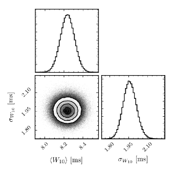
Figure 2: The estimated marginal posterior probability distributions for the noise-only model parameters of the beam-width data.

In Fig. 3 we plot the maximum posterior estimate (MPE) of the signal alongside the data, i.e. the model prediction when the parameters are set equal to the peak values of the posterior probability distributions. This figure demonstrates that, for the noise-only model, the observed $W_{10}$ has a mean value of approximately $8$ ms, then all the variations about this mean are due to the noise. In the following section we will develop models where at least some the variation is explained by periodic modulations.

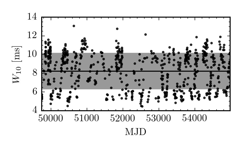
Figure 3: Posterior predictive check of the fit of the noise-only model posterior distribution to the data: the solid black line is the maximum posterior estimate (MPE), i.e. the model prediction when the parameters are set equal to the values corresponding to the peaks of the posterior probability distributions. The shaded region indicates the MPE of the 1-$\sigma_{W_{10}}$ noise about the beam-width model, black dots are the original data.

3.2 Switching model

The switching idea is phenomenological and we will build the model based on the modification of Lyne et al. (2010) by Perera et al. (2015): that is we assume the magnetosphere switches between two meta-stable states twice during a single period (the motivation for this is discussed in Sec. 3.2.1). For this work we will assume the switching to be deterministic, although improvements could be made by allowing the switching time to dither, or probabilistic variations in the switching states themselves; see Lyne et al. (2010) for some exploration of such ideas. This fully deterministic model captures the primary features without explaining the underlying physics, for example the cause of the switching. Both Jones (2012) and Cordes (2013) have worked to improve the physical motivations for the switching and provide a consistent picture. Nevertheless, in this work we choose to use the simple phenomenological model as a basis, which can be improved upon in future work.

3.2.1 Defining the spin-down rate model

The model proposed by Lyne et al. (2010) poses two states for the magnetosphere which we will label as $S_{1}$ and $S_{2}$. Then associated to each of these states is a corresponding spin-down rate $\dot{\nu}_{1}$ and $\dot{\nu}_{2}$. The smoothly varying spin-down that we observe is a result of the time-averaging process required to measure the spin-down rate. Lyne et al. (2010) suggested a square-wave-like switching with a duty rate measuring the fraction of time spent in one state compared to the other. They also proposed a dither in the switching period which will obscure the periodicity, and may give rise to low-frequency structure; we will not consider the dither in this work, but will investigate it in future work. While studying PSR B0919+06, which also demonstrates a double-peaked spin-down rate like B1828-11, the authors of Perera et al. (2015) realised that a (deterministic) switching model which flips once per cycle is incapable of explaining the double-peak observed in the spin-down rate (in particular that one peak is systematically smaller than the other). In order to explain this double-peaked structure, they propose that the mode-changes responsible for switching in the spin-down rate must be doubly-periodic: that is the spin-down rate changes state twice during a single cycle. Other modifications, such as introducing a third magnetospheric state, are possible, but in this work we will apply the Perera et al. (2015) switching model to B1828-11.

We now discuss the particular formulation of this model used in this analysis, firstly defining the underlying spin-down model and then the time-averaging process. To aid in this discussion we plot both the underlying spin-down model and time-average in Fig. 4 and gradually introduce each feature.

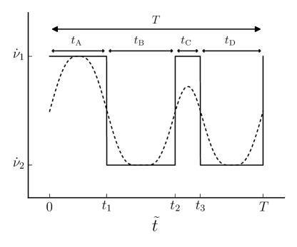
Figure 4: Schematic of the doubly-periodic spin-down rate model proposed by Perera et al. (2015). The solid line is the underlying spin-down evolution while the dashed line indicates the measured time-averaged quantity. In this instance, the time-average window is longer than $t_{\mathrm{C}}$, but shorter than the other three durations.

We begin by defining $\tilde{t}=(t-t_{\mathrm{ref}})+\phi_{0}T\mod(T)$ where $\phi_{0}\in[0,1]$ is an arbitrary phase offset and $t_{\mathrm{ref}}$ is a reference time. For all models in this study we will set $t_{\mathrm{ref}}=$ MJD 49621 to coincide with the epoch at which the ATNF database Manchester & Lyne (1977) records measurements for B1828-11. Then the function which generates the switching is

$$\dot{\nu}_{\mathrm{u}}(t)=\left\{\begin{array}[]{ccc}\dot{\nu}_{1}&\mathrm{if}&0<\tilde{t}<t_{1}\textrm{ or }t_{2}<\tilde{t}<t_{3}\\ \dot{\nu}_{2}&\mathrm{if}&t_{1}<\tilde{t}<t_{2}\textrm{ or }t_{3}<\tilde{t}<T\\ \end{array}\right.,$$ (12)

where the subscript ‘u’ denotes that this is the underlying spin-down model.

There are multiple ways to parametrize the switching times in the model. For the data analysis, we have chosen to parametrize by the total cycle duration $T$ and three of the segment durations $t_{\mathrm{A}}$, $t_{\mathrm{B}}$ and $t_{\mathrm{C}}$.

This model is subject to label-switching degeneracy in the choice of $\dot{\nu}_{1}$ and $\dot{\nu}_{2}$ and also between the various time-scales and initial phase $\phi_{0}$. This degeneracy may cause difficulties in the MCMC search algorithm, and we therefore fix this gauge freedom by specifying that $|\dot{\nu}_{1}|<|\dot{\nu}_{2}|$, $t_{\mathrm{A}}\geq t_{\mathrm{C}}$, and we require that $t_{\mathrm{A}}$ refers to a segment where $\dot{\nu}=\dot{\nu}_{1}$.

Based on a cursory inspection of the observed B1828-11 spin-down rate (see Fig. 1 panel A), it is clear that the secular second-order spin-down rate is non-zero. To model this we will include a constant $\ddot{\nu}$ in the underlying spin-down model

$$\dot{\nu}(t)=\dot{\nu}_{\mathrm{u}}(t)+\ddot{\nu}(t-t_{\mathrm{ref}})\,.$$ (13)

This gives the intrinsic spin-down rate of the pulsar which would be observed if measurements could be taken without time-averaging

To simulate the observed spin-down rate, we could time-average Eqn. (13) directly. Instead we choose to mimic the data collection process responsible for the time-averaging. Let us first discuss the data collection process as described by Lyne et al. (2010). Observers start with the time-of-arrival of pulsations, which is a measure of the pulsar rotational phase. Taking a 100 day window of data, starting at the earliest observation, a second-order Taylor expansion in the phase is fitted to the data yielding a measurement of $\dot{\nu}$. Then the processes is repeated, sliding the window in intervals of $25$ days over the whole data set. The measured $\dot{\nu}$ values at the centre of each window gives a time-averaged spin-down rate.

To mimic this data collection process, we first integrate Eqn. (13) twice to generate the phase and then repeat the above process. When integrating, we can ignore the arbitrary phase and frequency offsets since we discard them when calculating the spin-down rate. The resulting spin-down rates constitutes our signal model which is the time-average of Eqn. (13). A schematic representation of the sort of spin-down that is then found is given by the dotted curve in Figure Fig. 4. Clearly, the time-averaged spin-down is much smoother than than the underlying spin-down.

It is worth taking a moment to realise that the relation of the time-average spin-down to the underlying model $\dot{\nu}$ depends on both the segment durations and the length of the time average ($t_{\mathrm{ave}}=100$ days). For the $i^{th}$ segment, if the duration $t_{i}>t_{\mathrm{ave}}$ then the time-averaged spin-down will “saturate” and have a flat spot as in segment A of the illustration in Fig. 4. On the other hand, if $t_{i}<t_{\mathrm{ave}}$ then the maximum spin-down rate in this segment will be a weighted sum of the two underlying spin-down rates as in segment B of the illustration. The weighting is determined by the amount of time the underlying spin-down rate spends in each state during the time-average window.

3.2.2 Parameter estimation for the spin-down

In Table 1 we list the selected priors. For $\ddot{\nu}$ we define $\ddot{\nu}^{\tiny\mathrm{ATNF}}=(8.75\pm 0.09)\times 10^{-25}$ s^-3 (the value from the ATNF catalogue) and use a normal prior with this mean and standard deviation. In the tables we show the difference with respect to this value. For the remaining parameters we select uniform priors using crude estimates of the data in panel A of Fig. 1. As previously mentioned, this means we are using the data twice: once in setting up the priors and once for the fitting. Therefore it would be inappropriate to use the results in a model comparison and this is not our intention: we want to use the posterior distribution as a prior for the beam-width parameter estimation.

Table 1: Prior distributions for the spin-down switching model.

Parameter	Distribution	Units
$\dot{\nu}_{1}$	Unif(${\text{{-}}3.66}\times 10^{\textrm{-}13}$, ${\text{{-}}3.64}\times 10^{\textrm{-}13}$)	$\mathrm{s}^{\textrm{-}2}$
$\dot{\nu}_{2}$	Unif(${\text{{-}}3.67}\times 10^{\textrm{-}13}$, ${\text{{-}}3.66}\times 10^{\textrm{-}13}$)	$\mathrm{s}^{\textrm{-}2}$
$\ddot{\nu}$-$\ddot{\nu}^{\tiny\mathrm{ATNF}}$	$\mathcal{N}$(0, ${9.0}\times 10^{\textrm{-}27}$)	$\mathrm{s}^{\textrm{-}3}$
$T$	Unif(450, 550)	days
$t_{\mathrm{A}}$	Unif(0, 250)	days
$t_{\mathrm{B}}$	Unif(0, 250)	days
$t_{\mathrm{C}}$	Unif(0, 250)	days
$\phi_{0}$	Unif(0, 1)
$\sigma_{\dot{\nu}}$	Unif(0, ${1}\times 10^{\textrm{-}15}$)	$\mathrm{s}^{\textrm{-}2}$

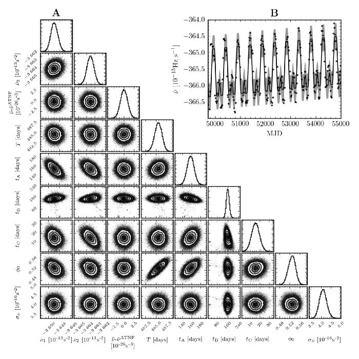
Figure 5: A: The estimated marginal posterior probability distribution for the Switching spin-down model parameters. B: Checking the fit of the model using the maximum posterior values to the data; see Fig. 3 for a complete description.

For the spin-down data under the switching model, the MCMC simulations converge quickly to unimodal and approximately Gaussian distributions. The distributions are plotted in Fig. 5A, and we summarise the results by their mean and standard-deviation in Table 2. In the case of parameters with uniform priors, this indicates that the data is informative and a well defined ‘best-fit’ has been selected. For $\ddot{\nu}$ the posterior has not departed significantly from the (informative) prior meaning that the data agrees with the prior.

Table 2: Posterior estimates for the spin-down switching model.

Parameter	Mean $\pm$ s.d.	Units
$\dot{\nu}_{1}$	${\text{{-}}3.6489}\times 10^{\textrm{-}13}$$\pm$${6.33}\times 10^{\textrm{-}17}$	$\mathrm{s}^{\textrm{-}2}$
$\dot{\nu}_{2}$	${\text{{-}}3.6635}\times 10^{\textrm{-}13}$$\pm$${4.44}\times 10^{\textrm{-}17}$	$\mathrm{s}^{\textrm{-}2}$
$\ddot{\nu}$-$\ddot{\nu}^{\tiny\mathrm{ATNF}}$	${\text{{-}}3.1051}\times 10^{\textrm{-}28}$$\pm$${9.0}\times 10^{\textrm{-}27}$	$\mathrm{s}^{\textrm{-}3}$
$T$	$485.52$$\pm$0.8649	days
$t_{\mathrm{A}}$	$157.75$$\pm$7.6587	days
$t_{\mathrm{B}}$	$159.71$$\pm$11.7798	days
$t_{\mathrm{C}}$	15.1379$\pm$4.3925	days
$\phi_{0}$	0.5278$\pm$0.0143
$\sigma_{\dot{\nu}}$	${4.0932}\times 10^{\textrm{-}16}$$\pm$${1.84}\times 10^{\textrm{-}17}$	$\mathrm{s}^{\textrm{-}2}$

To check that our fit is sensible, we plot the observed spin-down data in Fig. 5B alongside the maximum posterior estimate for the signal. The relative size of the noise component informs us how well the model fits the data: if $\sigma_{\dot{\nu}}$ is of a similar size to the variations in spin-down rate, then the model does poorly and we require a large noise component. In this case the noise-component is smaller than the variations in spin-down rate and the signal model explains most of the variations in the data.

Comparing the maximum posterior values of the four segment times to the baseline on which we time-average (fixed at 100 days) can give an insight into how the model has best fit the data. If we take the posterior of $t_{\mathrm{C}}$, we find it has a mean value of $\sim 15$ days which is significantly shorter than the baseline on which we time-average. For the other three segments, their durations are longer than this baseline. The reason that the fit in Fig. 5B has one maxima smaller than the other, is because the segment duration for that segment, $t_{\mathrm{C}}$, is shorter than the time-average baseline. This is expected and was precisely the motivation for using the model proposed by Perera et al. (2015); a switching model split into only two segments could not produce this feature.

3.2.3 Defining the beam-width model

For the beam-width, we assume that changes in the spin-down rate directly correlate to changes in this beam-width through changes in the beam geometry. Since we require the switching to be doubly-periodic for the spin-down to make sense, so we must require the beam-width to be doubly periodic. That is we define the beam-width model to be

$$W(t)\left\{\begin{array}[]{ccc}W_{1}&\mathrm{if}&0<\tilde{t}<t_{1}\textrm{ or }t_{2}<\tilde{t}<t_{3}\\ W_{2}&\mathrm{if}&t_{1}<\tilde{t}<t_{2}\textrm{ or }t_{3}<\tilde{t}<T\\ \end{array}\right..$$ (16)

Lyne et al. (2010) noted that the larger beam-widths tended to correlate with the lower (absolute) spin-down rate ($\dot{\nu}_{1}$ in our model). We could fix this by requiring that $W_{1}>W_{2}$ (recalling that we set $|\dot{\nu}_{1}|<|\dot{\nu}_{2}|$), but instead we will not implement such a constraint and allow the data to decide. As with the spin-down, to break the degeneracy in the times we will require again that $t_{\mathrm{A}}\geq t_{\mathrm{C}}$. We will not assume any secular changes in the beam-width for simplicity.

3.2.4 Parameter estimation for the beam-width

Having obtained a sensible fit to the spin-down data, we use the resulting posteriors (as summarised in Table 2) to inform our priors for the beam-width data. We can do this only for those parameters common to both the beam-width and spin-down predictions of the switching model: namely the four time-scales, and the phase-offset. We would like to relate the spin-down rates $\dot{\nu}_{1}$ and $\dot{\nu}_{2}$ to the beam-widths. However, the underlying physics is not understood, and so instead we will take a naive approach and set a prior on the beam-widths from astrophysical data.

For the beam-widths, $W_{1}$ and $W_{2}$, we will use the same prior as defined in Sec. 3.1.2 for the noise-only model: namely a uniform prior on $[0,0.1P^{\mathrm{ATNF}}]$ covering 10% of the spin-period. Using such a prior introduces some ambiguity into the model comparison as the result could be ‘tuned’ by varying the fraction $f$ of the spin-period used to set the uniform prior limits (here $f=0.1$). This issue is addressed in Sec. 4.3 where we find all sensible choices of $f$ lead to the same overall conclusion.

The final parameter which requires a prior distribution is the noise-component: as described in Sec. 3.1 we apply a prior to $\sigma_{W_{10}}$ using a crude estimate from the data; this is tabulated along with the other priors in Table 3.

Table 3: Prior distributions for the beam-width switching model. Parameters for which the prior is taken from spin-down posteriors are labelled by ^∗.

Parameter	Distribution	Units
$W_{1}$	Unif(0, 40.5000)	ms
$W_{2}$	Unif(0, 40.5000)	ms
$T$∗	$\mathcal{N}$($485.5$, 0.8649)	days
$t_{\mathrm{A}}$∗	$\mathcal{N}$($158.0$, 7.6587)	days
$t_{\mathrm{B}}$∗	$\mathcal{N}$($160.0$, 11.7798)	days
$t_{\mathrm{C}}$∗	$\mathcal{N}$(15.1379, 4.3925)	days
$\phi_{0}$∗	$\mathcal{N}$(0.5278, 0.0143)
$\sigma_{W_{10}}$	Unif(0, 5)	ms

We plot the posterior estimate in Fig. 6A which demonstrates non-Gaussianity and multimodal features in the segment times and the phase. This indicates the existence of multiple solutions which could explain the data. We note that the noise component $\sigma_{W_{10}}$ has a mode at 1.6 ms which is less than the 2ms required in the noise-only model. This indicates that some of the variability is being explained by the signal model.

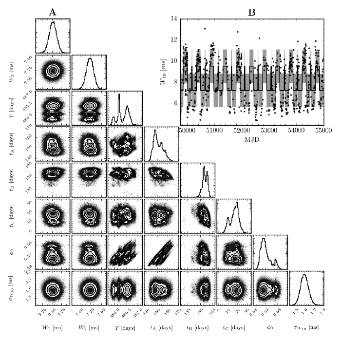
Figure 6: A: The estimated marginal posterior probability distribution for the Switching beam-width model parameters. B: Checking the fit of the model using the maximum posterior values to the data; see Fig. 3 for a complete description.

In Table 4 we summarise the posterior. We find that the posterior modes satisfy $W_{1}>W_{2}$: larger beam-widths are associated with the smaller absolute spin-down rates as found by Lyne et al. (2010).

Table 4: Posterior estimates for the beam-width switching model.

Parameter	Mean $\pm$ s.d.	Units
$W_{1}$	9.5166$\pm$0.0956	ms
$W_{2}$	7.2327$\pm$0.0830	ms
$T$	$485.04$$\pm$0.7286	days
$t_{\mathrm{A}}$	$150.98$$\pm$4.3909	days
$t_{\mathrm{B}}$	$155.29$$\pm$3.0598	days
$t_{\mathrm{C}}$	16.4134$\pm$4.5771	days
$\phi_{0}$	0.5409$\pm$${8.38}\times 10^{\textrm{-}3}$
$\sigma_{W_{10}}$	1.5964$\pm$0.0427	ms

Again we check the predictive power of our estimated posterior by plotting the MPE alongside the data in Fig. 6B. The fit to the data is not as good as the spin-down fit: by eye it is clear that most data points lie away from the signal model requiring a greater (relative) level of noise.

3.3 Precession model

We will now define the precession model and its predictions for the expected signal in the spin-down and beam-width data.

Classical free precession refers to the rotation of a rigid non-spherical body when there is a misalignment between its spin and rotation axes. For this work we will consider a biaxial star, acted upon by an electromagnetic torque as discussed in the next section. We will work with the angles defined in Jones & Andersson (2001): that is the star emits its EM radiation beam along the magnetic dipole $\mathbf{m}$ which makes an angle $\chi$ with the symmetry axis of the moment of inertia, and $\theta$ is the so-called wobble angle made between the symmetry axis and the angular momentum vector. We will consider the small-wobble angle regime where $\theta\ll 1$ since this is thought to be the most physical solution for B1828-11. Finally we define $P$ as the rotation period, and $\dot{P}$ its time derivative, where the small variations due to precession have been averaged over, and

$$\tau_{\mathrm{Age}}\equiv\frac{P}{\dot{P}}.$$ (17)

as a characteristic spin-down age.

3.3.1 Defining the spin-down rate model

Observers infer the spin-down rate by measuring the arrival times of pulsations. For a freely precessing star the spin-down rate is periodically modulated on a time-scale known as the free precession period, which we will denote as $\tau_{\mathrm{P}}$. This result is referred to as the geometric modulation (Jones & Andersson, 2001) since it is a geometric effect. Under the action of a torque the geometric effect persists, but an additional electromagnetic effect enters owing to torque variations (Cordes, 1993). The authors of Jones & Andersson (2001) and Link & Epstein (2001) studied both effects in the presence of a vacuum dipole torque (Davis & Goldstein, 1970) and agreed that the electromagnetic contributions dominate for B1828-11: we will therefore neglect the geometric effect. The precession model for B1828-11 has been developed by Akgün et al. (2006) where a non-vacuum dipole torque was considered and additionally by Arzamasskiy et al. (2015) where the effect of a plasma-filled magnetosphere was investigated. All of these are potential areas of improvement, but in this work we will restrict our focus to the simplest specification capable of explaining the observations. In particular, we will use a generalisation of the vacuum dipole torque to allow for a braking index $n\neq 3$, but retain the angular dependence; this ansatz may be written as

$$\dot{\nu}=-k\nu^{n}\sin^{2}\Theta,$$ (18)

where $k$ is a positive constant, and $\Theta$ is the polar angle between the dipole and the angular momentum vector as as calculated in Eqn. (52) of Jones & Andersson (2001). Then we calculate secular solutions in which $\Theta$ takes its fixed, time-averaged value. We denote by $\theta$ the angle between the symmetry axis of the moment of inertia and the angular momentum vector, and denote by $\chi$ the angle between the symmetry axis and the magnetic dipole m. We can then combine the secular solution with an expansion of $\sin^{2}\Theta$ in the small $\theta$ limit, to give a spin-down rate

$$\begin{split}\dot{\nu}(t)=\frac{1}{\tau_{\mathrm{Age}}P}&\left(-1+n\frac{1}{\tau_{\mathrm{Age}}}(t-t_{\mathrm{ref}})\right.\\ &+\theta\left.\left[2\cot\chi\sin\left(\psi(t)\right)-\frac{\theta}{2}\cos\left(2\psi(t)\right)\right]\right),\end{split}$$ (19)

where

$$\psi(t)=2\uppi\frac{t-t_{\mathrm{ref}}}{\tau_{\mathrm{P}}}+\psi_{0}.$$ (20)

As in the switching model, $t_{\mathrm{ref}}=\textrm{MJD }49621$. The first two terms are the secular spin-down rate and its first derivative. The term in the square brackets is the modulation and can be found from appropriate manipulation of Eqn. (58) and (73) in Jones & Andersson (2001), or Eqn. (20) in Link & Epstein (2001), aside from a factor of $\chi$ in the harmonic term which we believe to be a misprint.

For $\chi<\uppi/2$ the spin-down rate modulations are sinusoidal. When $\chi\approx\uppi/2$ (such that the star is nearly an orthogonal rotator), we will see a strong harmonic at twice the precession frequency. It is precisely this behaviour which is able to explain the doubly-peaked spin-down rate for B1828-11.

3.3.2 Parameter estimation for the spin-down

In Table 5 we list the priors selected for the spin-down precession model.

Table 5: Prior distributions for the spin-down precession model.

Parameter	Distribution	Units
$\tau_{\mathrm{Age}}$-$\tau_{\mathrm{Age}}^{\tiny\textrm{ATNF}}$	$\mathcal{N}$(0, 0.3169)	yrs
$n$-$n^{\tiny\textrm{ATNF}}$	$\mathcal{N}$(0, 0.1700)
$P$-$P^{\tiny\textrm{ATNF}}$	$\mathcal{N}$(0, ${1.2}\times 10^{\textrm{-}11}$)	s
$\tau_{P}$	Unif(450, 550)	days
$\theta$	Unif(0, 0.1)	rad
$\chi$	Unif($2\uppi/5$, $\uppi/2$)	rad
$\psi_{0}$	Unif(0, $2\uppi$)	rad
$\sigma_{\dot{\nu}}$	Unif(0, ${1}\times 10^{\textrm{-}15}$)	$\mathrm{s}^{\textrm{-}2}$

For $\tau_{\mathrm{P}}$ and $\sigma_{\dot{\nu}}$ we use a prior based on a crude estimate from the data. For the spin-down age, braking-index, and pulse period we use a normal prior taking the mean and standard deviation from B1828-11 measurements reported in the ATNF catalogue: the values are listed in Table 6. In the analysis, we present the posteriors of the difference to the means of these values for convenience.

Table 6: Measured and inferred values of the precession spin-down model parameters from the ATNF pulsar catalogue (Manchester et al., 2005), these are given at epoch MJD 49621

$P^{\mathrm{ATNF}}$	0.405043321630 $\pm 1.2\times 10^{-11}$ s
$n^{\mathrm{ATNF}}$	16.08 $\pm$ 0.17
$\tau_{\mathrm{Age}}^{\mathrm{ATNF}}$	213827.91 $\pm 0.32$  yrs

Finally for $\psi_{0}$ we give the full domain of possible values. Since our derivation of the signal models in Sec. 3.3 assumed the small wobble-angle regime $\theta\ll\chi$ and $\chi\sim\uppi/2$, we similarly restrict their uniform priors to the relevant range.

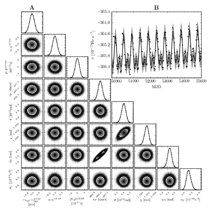
Figure 7: A: The estimated marginal posterior probability distribution for the precession spin-down model parameters. For the secular spin-down quantities, we show the difference with respect to the values as listed in table 6. B: Checking the fit of the model using the maximum posterior values to the data; see Fig. 3 for a complete description.

Running the MCMC simulations we plot the resulting posterior in Fig. 7 and provide a summary in Table 7. For all parameters the posterior distribution is Gaussian: in the case of parameters which we gave a uniform prior, this indicates that the spin-down data is informative. For the parameters using an informative prior (from the ATNF catalogue), the posterior and prior are similar, this indicates the data agrees with the prior, but does not significantly improve our estimates.

Table 7: Posterior estimates for the spin-down precession model. For the secular spin-down quantities, we report the posterior difference with respect to the values as listed in table 6.

Parameter	Mean $\pm$ s.d.	Units
$\tau_{\mathrm{Age}}$-$\tau_{\mathrm{Age}}^{\tiny\textrm{ATNF}}$	${7.461}\times 10^{\textrm{-}3}$$\pm$0.3159	yrs
$n$-$n^{\tiny\textrm{ATNF}}$	0.0199$\pm$0.1701
$P$-$P^{\tiny\textrm{ATNF}}$	${1.0436}\times 10^{\textrm{-}14}$$\pm$${1.19}\times 10^{\textrm{-}11}$	s
$\tau_{P}$	$485.56$$\pm$0.8188	days
$\theta$	0.0490$\pm$0.0020	rad
$\chi$	1.5517$\pm$0.0013	rad
$\psi_{0}$	3.8709$\pm$0.0697	rad
$\sigma_{\dot{\nu}}$	${4.0423}\times 10^{\textrm{-}16}$$\pm$${1.81}\times 10^{\textrm{-}17}$	$\mathrm{s}^{\textrm{-}2}$

In Fig. 7B we check the fit of the posterior for the spin-down data. The spin-down model fits to the data points well with only a small amount of noise required to explain the data.

The posterior distributions conditioned on the spin-down data (as summarised in Table 7) can be compared with the values reported in Table 2 of Link & Epstein (2001). When comparing it should be noted that we are considering a longer stretch of data which includes most, but not all of the period studied by Link & Epstein (2001). For the two angles $\chi$ and $\theta$, the fractional difference is 0.001 and 0.14 respectively while the precession periods differ by a fractional amount 0.05. Clearly the solution found here is similar to that found by Link & Epstein (2001).

3.3.3 Defining the beam-width model: Gaussian intensity

Modulation of the observed beam due to precession is a purely geometric effect. Fixing the beam-axis to coincide with the magnetic dipole $\mathbf{m}$ and following Jones & Andersson (2001), we define $\Theta$ and $\Phi$ as the polar and azimuthal angles of $\mathbf{m}$ with respect to a fixed Cartesian coordinate system with $z$ along the angular momentum vector J. The observer is fixed in the Cartesian coordinate system with a polar angle $\iota$ to J, and azimuth $\Phi_{\mathrm{obs}}$. The slow precessional motion of the spin-vector causes modulation in the angle $\Theta$:

$$\Theta(t)=\cos^{-1}\left(\sin\theta\sin\chi\sin\psi(t)+\cos\theta\cos\chi\right),$$ (21)

which, in the $\theta\ll 1$ limit is approximately

$$\Theta(t)\approx\chi-\theta\sin\psi(t).$$ (22)

Taking the plane containing the angular momentum vector and the observer, in Fig. 8 we demonstrate the range of motion of $\mathbf{m}$ over a precessional cycle by a gray shaded region. The region has a mean polar value of $\chi$ and a range of $2\theta$.

Figure 8: Illustration of the angles as the beam-axis $\mathbf{m}$ cuts the plane containing the observer and the angular momentum $\mathbf{J}$. The grey shaded region indicates the extent to which $\mathbf{m}$ varies over a precessional cycle.

For an observer fixed at an angle $\iota$ to J we define an impact parameter:

$$\Delta\Theta(t)=\Theta(t)-\iota,$$ (23)

which will vary in time with the precession period $\tau_{\mathrm{P}}$. This impact parameter determines how the observer’s line-of-sight cuts the emission beam; if $\Theta(t)$ varies due to changes in $\Delta\Theta(t)$, then the observer will measure the beam to vary on the slow precession time-scale. To help visualise the setup, in Fig. 9 we plot the unit sphere with points corresponding to the beam-axis $\mathbf{m}$ and the observer. For each of these we have added lines of latitude and longitude. Then we see that that $\Delta\Theta$ is the difference between the lines of latitude and we can also define $\Delta\Phi(t)=\Phi(t)-\Phi_{\textrm{obs}}$ as the difference in the lines of longitude.

Figure 9: The angular position of the observer and the magnetic dipole $\mathbf{m}$ on the unit sphere centered on the star; $\Delta\Theta$ and $\Delta\Phi$ are then the polar and azimuthal angles between them.

The analysis by Stairs et al. (2000) characterised the beam by a shape parameter. Link & Epstein (2001) used an expansion in $\Delta\Theta$ to model the beam-width and hence the shape-parameter. This allowed them to use their fit to the timing-data to infer the beam-geometry which they found to be hour-glass shaped; see their Figure 5 for a schematic illustration. The authors of Lyne et al. (2010) did not use a shape-parameter as it requires time-averaging over a longer base-line, something they wish to avoid in order to be able to observe the switching. Instead, they considered the beam-width at 10% of the maximum, $W_{10}$, which is measured on a shorter time-baseline ($\sim 1$ hr). If we want to use the beam-width to make a model comparison, we will require a model for $W_{10}$ that is not informed by the data.

The integrated pulse profile of B1828-11 (Fig. 4 of Lyne et al. (2010)) shows a single peak, often described as core emission (Lyne & Manchester, 1988). Since we do not have a detailed model of the emission mechanism, we will now consider the most rudimentary and natural beam geometry which fits this: a circularly symmetric (about the beam-axis) intensity which falls-of with a Gaussian function. Specifically, let us define $\Delta d$ as the central angle between the observer’s line-of-sight and the beam (this is the spherical distance between the two points marked in Fig. 9), then the intensity is

$$\mathcal{I}(t)=\mathcal{I}_{0}\exp\left(-\frac{\Delta d(t)^{2}}{2\rho^{2}}\right).$$ (24)

Here $\mathcal{I}_{0}$ is the intensity when observed directly along the dipole and $\rho$ measures the angular width of the beam. From the spherical law of cosines, for an observer located at $(\Phi_{\mathrm{obs}},\iota)$, we have

$$\Delta d(t) =\cos^{-1}\left[\cos\Theta(t)\cos\iota+\sin\Theta(t)\sin\iota\cos|\Delta\Phi(t)|\right].$$ (25)

The observer will see a maximum pulse intensity at $\Delta\Phi=0$, given by

$$\mathcal{I}_{\textrm{max}}=\mathcal{I}_{0}\exp\left(-\frac{\left(\Theta(t)-\iota\right)^{2}}{2\rho^{2}}\right).$$ (26)

Now let us recognise that $\Theta$ varies on the slow precession time-scale, while $\Phi$ varies on the rapid spin time-scale: a single pulse consists of $\Phi$ varying between $\Phi_{\mathrm{obs}}-\uppi$ and $\Phi_{\mathrm{obs}}+\uppi$. So over a single pulse, we can treat $\Theta$ as a constant. The pulse width $W_{10}$, as measured by observers, is the duration for which the pulse intensity is greater than 10% of the peak observed intensity. For a single pulse, we can define this duration as the period for which the inequality

$$\mathcal{I}>\mathcal{I}_{\textrm{max}}\frac{1}{10},$$ (27)

is satisfied. Substituting equations (24) and (26) into (27) and rearranging we find that

$$\cos(|\Delta\Phi(t)|)>\frac{\cos\Psi(t)-\cos\Theta(t)\cos\iota}{\sin\Theta(t)\sin\iota},$$ (28)

where

$$\Psi(t)=\sqrt{\left(\Theta(t)-\iota\right)^{2}+2\rho^{2}\ln\left(10\right)}.$$ (29)

Since we treat $\Theta$ as a constant over a single pulsation, we can also treat the whole right-hand-side of the inequality as a constant during each pulse.

Now consider a single rotation with the magnetic dipole starting and ending in the antipodal point to the observer’s position such that $\Delta\Phi(t)$ increases between $-\uppi$ and $\uppi$ during this rotation. Then inequality (28) measures the fraction of the pulse corresponding to the beam-width measurement. In terms of the rotation, we define $\delta\Phi$ as the angular width for which the inequality is satisfied and calculate it to be

$$\delta\Phi(t)=2\cos^{-1}\left(\frac{\cos\Psi(t)-\cos\Theta\cos\iota}{\sin\Theta\sin\iota}\right).$$ (30)

Then the beam-width is

$$W_{10}(t)=P\frac{\delta\Phi(t)}{2\uppi},$$ (31)

from which we arrive at

$$W_{10}(t)=\frac{P}{\uppi}\cos^{-1}\left(\frac{\cos\Psi(t)-\cos\Theta(t)\cos\iota}{\sin\Theta(t)\sin\iota}\right).$$ (32)

In order for the observer to measure the width at 10% of the maximum, the beam intensity must of course drop below this value before increasing again. In reality we typically observe pulse durations lasting for small fractions of the period, especially when they are close to orthogonal rotators (Lyne & Manchester, 1988).

To set a prior on $\rho$ we consider a special case in which the polar angle of the beam and the observer are at the equator ($\Theta=\iota=\uppi/2$). From our spin-down analysis, we know the first of these conditions is true for B1828-11 since $\chi$ is close to $\uppi/2$. The second condition is based on the assumption that the observer would not see a tightly pulsed beam if they are not close to the polar angle of the beam. In this special instance, inserting Eqn. (29) into Eqn. (32), the beam-width is

$$W_{10}\bigg{|}_{\Theta=\iota=\uppi/2}=\frac{P}{\uppi}\sqrt{2\ln 10}\rho.$$ (33)

To set a prior on $\rho$, we can equate this with the beam-widths used in the switching model, for which we set a uniform prior from $0$ to $0.1P^{\mathrm{ATNF}}$. To make an even-handed comparison we will therefore set a uniform prior on $\rho$ from 0 to

$$\frac{\uppi}{10\sqrt{2\ln 10}}\approx 0.15,$$ (34)

so that, for this special case, the prior range of $\rho$ corresponds exactly to the prior range of the beam-widths in the switching model. This prior range will change, but not by orders of magnitude when considering a system close to, but not exactly at, this special case. Therefore this prior assures that the model comparison does not introduce any significant bias into the model comparison.

3.3.4 Parameter estimation for the Gaussian beam-width model

We are in a position to fit the Gaussian beam model to the observed $W_{10}$ values. In Table 8 we list the priors taken from the spin-down fit along with three additional priors. For $\iota$ we choose a uniform prior in $\cos\iota$ on $[-1,1]$, this corresponds to allowing $\iota$ to range from $[0,\uppi]$ (the observer could be in either hemisphere); for $\rho$ we apply the prior from Eqn. (34); and for $\sigma_{W_{10}}$ we use a crude estimate based on the data (again we use the same prior for all three models).

Table 8: Prior distributions for the beam-width Gaussian precession model. Parameters for which the prior is taken from spin-down posteriors are labelled by ^∗.

Parameter	Distribution	Units
$\tau_{P}$∗	$\mathcal{N}$($485.6$, 0.8188)	days
$P$-$P^{\tiny\textrm{ATNF}}$ ∗	$\mathcal{N}$(${1.04}\times 10^{\textrm{-}14}$, ${1.19}\times 10^{\textrm{-}11}$)	s
$\theta$∗	$\mathcal{N}$(0.0490, 0.0020)	rad
$\chi$∗	$\mathcal{N}$(1.5517, 0.0013)	rad
$\psi_{0}$∗	$\mathcal{N}$(3.8709, 0.0697)	rad
$\rho$	Unif(0, 0.1500)	rad
$\cos(\iota)$	Unif(-1, 1)
$\sigma_{W_{10}}$	Unif(0, 5)	ms

Fitting Eqn. (32) to the data we discover that the Gaussian beam model is a poor fit to the data. In Fig. 10B the MPE shows that while the model is able to fit the averaged beam-width, it cannot simultaneously fit the amplitude of periodic modulations.

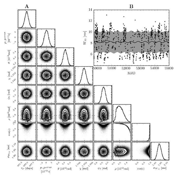
Figure 10: A: The estimated marginal posterior probability distribution for the Gaussian spin-down model parameters. B: Checking the fit of the model using the maximum posterior values to the data; see Fig. 3 for a complete description.

The posterior distribution (as seen in Fig. 10A) is Gaussian for all of the parameters except $\cos\iota$ for which it concentrates the probability at $\iota\approx 0$: the observer looks almost down the angular momentum vector. Since $\chi\approx\uppi/2$ and $\theta\ll 1$, for each pulsation the beam must therefore sweep out a cone with such a large opening angle it is close to a plane orthogonal to the rotation vector. Meanwhile the rotation vector is nearly parallel to the angular momentum, since $\theta\ll 1$. As a result, the beam remains approximately orthogonal to the observer for the entirety of each pulsation. We find this result difficult to believe on the grounds that the observer would not see tightly coliminated pulsed emission. For this reason, we conclude that the Gaussian beam-intensity fails to fit the data because the best-fit is unphysical. In retrospect, this result is not surprising since a Gaussian beam intensity is known to have a beam-width (as measured by $W_{10}$) which is independent of the impact angle as discussed by Akgün et al. (2006). This is a direct result of measuring the beam-width with respect to the observed maximum and the self-similar nature of the Gaussian intensity under changes in the impact parameter.

3.3.5 Refining the beam-width model: modified-Gaussian intensity

As we have demonstrated that the Gaussian beam is unable to explain both the observed variations and average beam-width we must now consider how it could be varied in a natural way which does explain the data. One suggestion from Akgün et al. (2006) is to impose a sharper cut-off, or introduce a conal component in addition to the Gaussian core emission. We will follow a slightly different path below, one which represents a less drastic modification of the beam profile.

The beam intensity described by Eqn. (24) is circularly symmetric about the beam axis as viewed on the surface of the sphere. In the context of the hollow-beam model (Radhakrishnan & Cooke, 1969), Narayan & Vivekanand (1983) found that pulsar beams can be elongated with the ratio of major to minor axis being $\sim 3$ for typical pulsars. B1828-11 does not fit into the hollow-beam model (having only a single core component), but nevertheless if the conal emission can be non-circular a generalisation of our core intensity would be to allow for an elliptical beam.

To consider non-symmetric geometries, let us take the planar limit of Eqn. (25) by applying small angle approximations in $\Delta d,\Delta\Theta$ and $\Delta\Phi$:

$$\Delta d(t)^{2}=\Delta\Theta(t)^{2}+\sin\Theta(t)\sin\iota\Delta\Phi(t)^{2}.$$ (35)

This corresponds to setting the observer close to $\mathbf{m}$ in Fig. 9.

Obviously $\Delta\Phi$ ranges over $[0,2\uppi]$ in each rotation, but when $\Delta\Phi$ is not small, the intensity vanishes rapidly due to the Gaussian beam shape Eqn. (26). Therefore, Eqn. (35) is a good approximation for the separation when the beam is pointing near to the observer, while away from this it is a poor approximation, but the intensity is negligible and so the differences are inconsequential.

We can now allow for an elliptical beam geometry by postulating the beam intensity to be

$$\mathcal{I}(t)=\mathcal{I}_{0}\exp\left(-\frac{-\Delta\Theta(t)^{2}}{2\rho_{1}^{2}}-\frac{(\sin\Theta(t)\sin\iota\Delta\Phi(t))^{2}}{2\rho_{2}^{2}}\right).$$ (36)

Then to calculate the beam-width, we first find the maximum:

$$\mathcal{I}_{\textrm{max}}=\mathcal{I}_{0}\exp\left(-\frac{-\Delta\Theta(t)^{2}}{2\rho_{1}^{2}}\right).$$ (37)

Solving for the beam-width we find

$$W_{10}(t)=\frac{P}{\uppi}\frac{\sqrt{2\ln 10}\rho_{2}}{\sin\Theta(t)\sin\iota},$$ (38)

which is independent of $\rho_{1}$, the latitudinal standard-deviation. The extra degree of freedom introduced in Eqn. (36) is irrelevant to the beam-width measure because $W_{10}$ is defined by the ratio of the intensity to that at the observed peak $\mathcal{I}_{\textrm{max}}$.

This loss of a degree of freedom means that Eqn. (38) is an equivalent to an expansion of Eqn. (32) in the planar limit (i.e. the non-circular nature introduced by Eqn. (36) does not manifest in the prediction for $W_{10}$) and so will suffer the same problems if fitted to the data. To further generalise our intensity model we will therefore modify the beam-geometry by allowing a varying degree of non-circularity. This is done by expanding the longitudinal standard deviation as

$$\rho_{2}(t)=\rho_{2}^{0}+\rho_{2}^{\prime\prime}\Delta\Theta(t)^{2}.$$ (39)

Note that we have neglected to include a linear term here, forcing the geometry to be longitudinally symmetric about the beam-axis. Preliminary studies began by fitting a linear term only (this giving a modulation at the frequency $1/\tau_{\mathrm{P}}$), but it was found that including a second-order term (which provides modulation at both $1/\tau_{\mathrm{P}}$ and $2/\tau_{\mathrm{P}}$) gave a better fit. Including both terms, we found that the data was unable to provide inference on both $\rho_{2}^{\prime}$ and $\rho_{2}^{\prime\prime}$ due to degeneracy. In light of this, we drop the first term, but keep the second, which we feel is the simplest model which is able to fit the data.

Solving for the beam-width (i.e. with Eqn. (39) substituted into Eqn. (36)) we obtain a signal model

$$W_{10}(t)=\frac{P}{\uppi}\sqrt{\frac{2\ln 10}{\sin\Theta(t)\sin\iota}}\left(\rho_{2}^{0}+\rho_{2}^{\prime\prime}\Delta\Theta(t)^{2}\right),$$ (40)

which we will refer to as the modified-Gaussian precession beam-width model.

3.3.6 Parameter estimation for the modified-Gaussian precession beam-width

For equation (40), we give the relevant prior distributions in Table 9. As in the previous Gaussian model, we let $\iota$ range over $[0,\uppi]$; for $\rho_{2}^{0}$, we apply the prior on intensity widths as given by Eqn. (34); and for $\rho_{2}^{\prime\prime}$ we will use a normal prior with zero mean favouring a Gaussian intensity. The standard-deviation of this prior can have a measurable impact on the inference: if it is too small then the degree of freedom introduced by Eqn. 39 is effectively removed. Instead we want to make it significantly larger than the (apriori unknown) posterior value of $\rho_{2}^{\prime\prime}$: this generates a so-called non-informative prior. To set the prior standard-deviation then, we need to provide a rough scale for what value $\rho_{2}^{\prime\prime}$ should have. To do this we will define our prior expectation such that

$$\rho_{2}(\Delta\Theta=\rho_{2}^{0})\sim 2\rho_{2}^{0},$$ (41)

which is to say we expect $\rho_{2}$ to increase by no more than a factor of order unity over angular distances of the beam-width comparable to $\rho_{2}^{0}$ (the beam-width when the observer cuts directly through the beam-axis). This amounts to assuming that the beam does not depart very far from circularity. Plugging this into Eqn. (39), we get

$$\rho_{2}^{\prime\prime}\sim\frac{1}{\rho_{2}^{0}}.$$ (42)

From this, we use the upper limit from the uniform prior on $\rho_{2}^{0}$ (as calculated in Eqn. (34)), to set the standard-deviation for $\rho_{2}^{\prime\prime}$ at $1/0.15\approx 7$. We also tested different choices of $\rho_{2}^{\prime\prime}$ and found that the posteriors and odds-ratios where robust to the choice, provided the standard-deviation did not exclude the posterior value reported in table 10.

Table 9: Prior distributions for the beam-width modified-Gaussian precession model. Parameters for which the prior is taken from spin-down posteriors are labelled by ^∗.

Parameter	Distribution	Units
$\tau_{P}$∗	$\mathcal{N}$($485.6$, 0.8188)	days
$P$-$P^{\tiny\textrm{ATNF}}$ ∗	$\mathcal{N}$(${1.04}\times 10^{\textrm{-}14}$, ${1.19}\times 10^{\textrm{-}11}$)	s
$\theta$∗	$\mathcal{N}$(0.0490, 0.0020)	rad
$\chi$∗	$\mathcal{N}$(1.5517, 0.0013)	rad
$\psi_{0}$∗	$\mathcal{N}$(3.8709, 0.0697)	rad
$\rho_{2}^{0}$	Unif(0, 0.1464)	rad
$\rho_{2}^{\prime\prime}$	$\mathcal{N}$(0, 6.8308)	rad${}^{\textrm{-}2}$
$\cos(\iota)$	Unif(-1, 1)
$\sigma_{W_{10}}$	Unif(0, 5)	ms

The MCMC simulations converge quickly to a Gaussian distribution as shown in Fig. 11A and the posterior is summarised in Table. 10. The model parameters common to the spin-down model do not vary significantly from the spin-down posterior: this indicates the two models are consistent. We find that $\iota$ is close to $\uppi/2$ as expected, $\rho_{2}$ is sufficiently small indicating a narrow pulse beam, but $\rho_{2}^{\prime\prime}$ has departed from its prior mean of zero. This confirms that our generalisation of the Gaussian intensity, Eqn. (39), is important in fitting the data.

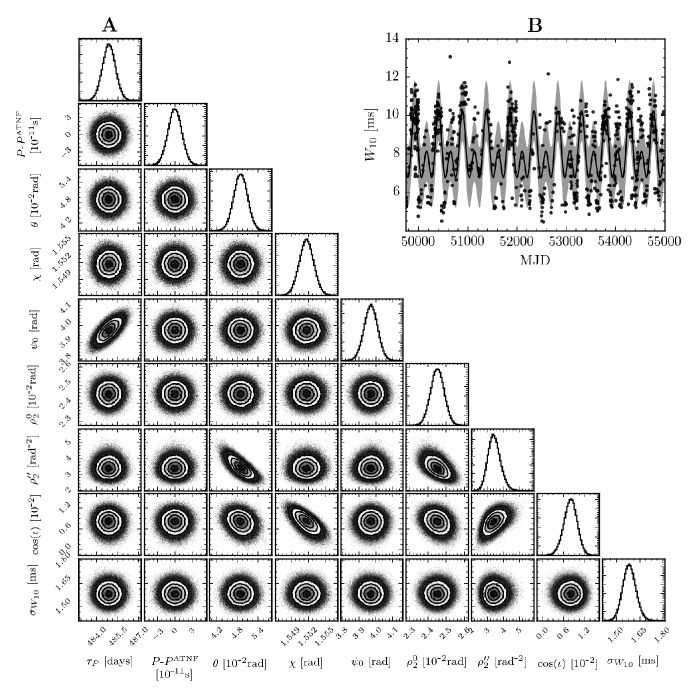
Figure 11: A: The estimated marginal posterior probability distribution for the modified-Gaussian precession beam-width model parameters. B: Checking the fit of the model using the maximum posterior values to the data; see Fig. 3 for a complete description.

Table 10: Posterior estimates for the beam-width modified-Gaussian precession model.

Parameter	Mean $\pm$ s.d.	Units
$\tau_{P}$	$484.87$$\pm$0.4706	days
$P$-$P^{\tiny\textrm{ATNF}}$	${\text{{-}}1.7719}\times 10^{\textrm{-}13}$$\pm$${1.19}\times 10^{\textrm{-}11}$	s
$\theta$	0.0490$\pm$0.0020	rad
$\chi$	1.5517$\pm$0.0013	rad
$\psi_{0}$	3.9701$\pm$0.0403	rad
$\rho_{2}^{0}$	0.0245$\pm$0.0004	rad
$\rho_{2}^{\prime\prime}$	3.4421$\pm$0.3878	rad${}^{\textrm{-}2}$
$\cos(\iota)$	${7.9326}\times 10^{\textrm{-}3}$$\pm$${1.9}\times 10^{\textrm{-}3}$
$\sigma_{W_{10}}$	1.5833$\pm$0.0422	ms

In Fig. 11B we perform the posterior predictive check plotting the MPE alongside the data. This demonstrates that the best-fit puts $\chi$ within $\theta$ of $\iota$ such that during the precessional cycle the beam-axis passes twice through observer’s location. This corresponds to the gray region in Fig. 8 intersecting the observer’s line-of-sight. When this happens, the modulation of the beam-width picks up a second harmonic at twice the precession frequency. The minima in Fig. 11B corresponds to the point in the precessional phase when the beam-axis point directly down the observer’s line-of-sight.

3.3.7 Recreating the beam-geometry

Since we have defined a beam-intensity in Eqn. (36) we can recreate the beam-geometry and pulse-shape from our MPE values. The data we have does not provide information about the latitudinal beam-shape parameter $\rho_{1}$; therefore we consider that there are a family of beam-geometries parametrized by $\rho_{1}=\lambda\rho_{2}^{0}$ where $\lambda$ is an arbitrary scale parameter and $\rho_{2}^{0}$ is the MPE value.

In figure 12 we pick four illustrative values for $\lambda$ and plot the resulting beam-geometry as contour lines at fixed fractions of the maximum beam intensity (which occurs at the origin). This demonstrates that the beam-geometry has an hour-glass shape in agreement with Link & Epstein (2001), although this becomes weaker with smaller values for $\lambda$.

In Fig. 12, a pulse corresponds to a horizontal cut through the intensity at fixed $\Delta\Theta$. Our posterior distribution, Fig. 11A, also provides information on how the observations cut through this beam-geometry. Under the precession hypothesis, the observer has a time-averaged $\Delta\Theta$ of $\chi-\iota$: this has been plotted as a horizontal dashed line in Fig. 12. Precession modulates $\Delta\Theta$ about this average value by $\pm\theta$; the observer’s line-of-sight through the beam therefore varies by $2\theta\approx 0.1$ rad over a precessional cycle. We have plotted a gray shaded region in Fig. 12 to show the extent, $\chi-\iota\pm\theta$, over which $\Delta\Theta$ varies during a precessional cycle.

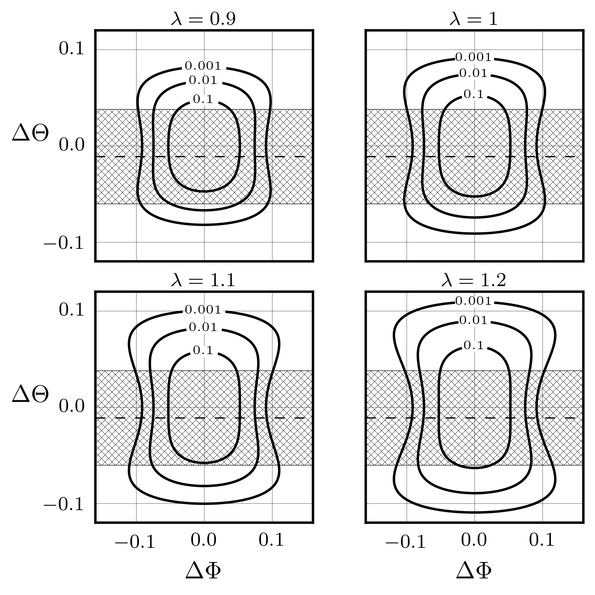
Figure 12: Recreating the beam geometry from the MPE of the modified-Gaussian precession beam-width model parameters for four different values of $\lambda$. Thick black lines indicate contour lines of the intensity function at fractions of the maximum intensity. The hatched area indicates the region of horizontal cuts (pulses) sampled by the observer: this has a mean, $\chi-\iota$, close to zero (marked by a dashed line) and varies by $\pm\theta$ about this mean.

We stress here that the contour lines cannot be used directly to measure the beam-width $W_{10}$. This is because $W_{10}$ is defined as the width at 10% of the peak intensity for that observed pulse and not the maximum intensity of the beam. The peak intensity for an observed pulse (a horizontal slice) is the intensity at $\Delta\Phi=0$ and it is with respect to this, which $W_{10}$ is measured.

By construction, the four beam geometries in Fig. 12 all produce the same $W_{10}$ behaviour as observed in Fig. 11B. The reason for this is that we have lost information on the total intensity by using $W_{10}$; other measurements of the beam-width could potentially yield more information and better constrain the beam geometry.

Fixing $\lambda=1$ we can also consider the variations in the pulse profile. In Fig. 13 we plot the normalised intensity for three values of $\Delta\Theta$ corresponding to the mean, and edges of the gray region in Fig. 12.

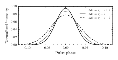
Figure 13: Recreating the pulse profiles for three particular slices through the beam using a fixed value of $\lambda=1$.

This figure shows that the narrow beam-widths occur when $\Delta\Theta$ is small, which, since $\chi$ is close to $\uppi/2$ coincide with the larger (absolute) spin-down rates. This agrees with the findings of Lyne et al. (2010) and this figure can be directly compared with panel C in Fig. 3 of that work.

4 Estimating the odds-ratio

4.1 Thermodynamic integration

Having checked that our MCMC simulations are a reasonable approximation to the posterior distribution we now calculate the marginal likelihood for each model and then their odds-ratio. To calculate the marginal likelihood we will use thermodynamic integration. This requires running $N$ parallel MCMC simulations and raising the likelihood to a power $1/T$ where $T$ is the ‘temperature’ of the chain. This method was originally proposed by Swendsen & Wang (1986) to improve the efficiency of MCMC simulations for multimodal distributions. In this work we use this method not to help with the efficiency of the simulations , but instead so that we can apply the method prescribed by Goggans & Chi (2004) to estimate the evidence as follows.

First we define the inverse temperature $\beta=1/T$, then let the marginal likelihood as a function of $\beta$ be

$$Z(\beta)=\int P(\textrm{data}|\boldsymbol{\theta})^{\beta}P(\boldsymbol{\theta})d\boldsymbol{\theta}.$$ (43)

When $\beta=1$, this gives exactly the marginal likelihood first defined in Eqn. (3). After some manipulation we see that

$$\frac{1}{Z}\frac{\partial Z}{\partial\beta}=\frac{\int\ln(P(\textrm{data}|\boldsymbol{\theta})P(\textrm{data}|\boldsymbol{\theta})^{\beta}P(\boldsymbol{\theta})d\boldsymbol{\theta}}{\int P(\textrm{data}|\boldsymbol{\theta})^{\beta}P(\boldsymbol{\theta})d\boldsymbol{\theta}}.$$ (44)

From this, we note that the right-hand-side is an average of the log-likelihood at $\beta$ and so

$$\frac{\partial}{\partial\beta}\left(\ln(Z)\right)=\langle\ln(P(\textrm{data}|\boldsymbol{\theta}))\rangle_{\beta}.$$ (45)

Using the likelihoods calculated in the MCMC simulations, we numerically integrate the averaged log-likelihood over $\beta$ which yields an estimation of the marginal likelihood. To be confident that the estimate is correct, we ensure that we use a sufficient number of temperatures and that they cover the region of interest.

4.2 Results

Applying the thermodynamic integration technique to all the models, we estimate the evidence for each model. Taking the ratio of the evidences gives us the Bayes factor and since we set the ratio of the prior on the models to unity, the Bayes factor is exactly the odds ratio (see Eqn. (2)).

We present the $\log_{10}\textrm{odds-ratio}$ between the models in Table 11. A positive value indicates that the data prefers model A over model B. Note that the error here is an estimate of the systematic error due to the choice of $\beta$ values (see Foreman-Mackey et al., 2013, for details).

Table 11: Tabulated log-odds-ratios for all models. ^∗By the precession model here we mean the precession with a modified Gaussian beam model as discussed in Sec. 3.3.5.

Model A	Model B	$\log_{10}(\textrm{odds-ratio})$
switching	noise-only	$57.4\pm 0.5$
precession∗	noise-only	$60.1\pm 0.5$
precession∗	switching	$2.7\pm 0.5$

This table allows quantitative discrimination amongst the models. The first two rows compare the switching and modified-Gaussian precession models against the noise-only model with the periodic modulating models being strongly preferred in both cases. Then in the last row we present the log-odds-ratio between the modified-Gaussian precession and switching model which shows that the data prefers the precession Modified Gaussian model by a factor $10^{2.7}$. Using the interpretation of Jeffreys (1998), the strength of this evidence can be interpreted as ‘decisive’ in favour of this precession model. For completeness, we also mention that the odds-ratio for the non-modified Gaussian model (which failed to fit the data in a physically meaningful way) against the noise-only model was $3.1\pm 0.6$.

4.3 Effect of the choice of prior

For both beam-widths in the switching model we used uniform priors on $[0,fP^{\mathrm{ATNF}}]$ with $f=0.1$ and these were transformed to also provide a fair prior on $\rho_{2}^{0}$ and $\rho_{2}^{\prime\prime}$. This choice of $f$ was taken from the upper limit quoted in Lyne & Manchester (1988) for typical values of the pulse width. Nevertheless, changing $f$ can have a measurable impact on the odds-ratio and so we will now study this effect.

To begin, we rewrite Eqn. (3), the marginal likelihood, by factoring out the $N$ parameters which have a uniform prior

$$P(\textrm{data}|\mathcal{M}_{i})=\frac{1}{\prod_{i}^{N}(b_{i}-a_{i})}\int P(\textrm{data}|\boldsymbol{\theta},\mathcal{M}_{i})P(\boldsymbol{\theta}^{*}|\mathcal{M}_{i})d\boldsymbol{\theta},$$ (46)

where by $P(\boldsymbol{\theta}^{*}|\mathcal{M}_{i}$) we mean the probability distribution of all remaining parameters which are not factored out, and $[a_{i},b_{i}]$ is the range for the $i^{th}$ uniform parameter. For the switching beam-width, the prefactor of this integral (factoring out the prior on $W_{1}$ and $W_{2}$) is $(fP^{\mathrm{ATNF}})^{-2}$: varying $f$ directly impacts the evidence for the switching model. For the precession model, we cannot factor the dependence on $f$ in the same way as we use a central normal prior on $\rho_{2}^{\prime\prime}$. We set the standard-deviation of this prior by applying Eqn. (42) so that it is inversely proportional to $f$. If both the prior on $\rho_{2}^{0}$ and $\rho_{2}^{\prime\prime}$ had been proportional to $f$ we would have an exact cancellation in the odds-ratio and hence no dependence on $f$. This is not the case and due to our prior on $\rho_{2}^{\prime\prime}$ the odds-ratio will depend on $f$.

To test the dependence, in Fig. 14 we plot the log odds-ratio as a function of $\log_{10}(f)$ (note that $f=0.1$ corresponds to the result in Table. 11). There are several features to understand. First, for $f\lesssim 0.024$ the odds-ratio rapidly grows, favouring precession; this is because for such small values of $f$ the beam-width switching prior excludes the values of $W_{1}$ required to fit the data. As a result the switching solutions are unnaturally disadvantaged compared to the precession solutions, such odds-ratios do not fairly compare the models.

For $0.024\lesssim f\lesssim 0.3$ the log-odds-ratio is approximately linear growing from $1.44$ when $f=0.24$ to $3.21$ when $f=0.3$. In this region the solutions for both models are supported by the prior in that it does not exclude or disfavour the posterior value. The variation in the odds-ratio results from changes in the prior volume of the switching model, the evidence for the precession model is constant in this region. Small $f$ values maximally constrains the prior volume for the switching model (without excluding posterior values) and hence give the greatest weight of evidence to switching and the smallest odds-ratios. For larger $f$ values the log of the prior volume grows linearly resulting in the observed growth.

For $f\gtrsim 0.3$ our choice of standard-deviation for $\rho_{2}^{\prime\prime}$ starts to disfavour the posterior value because it is inversely proportional to $f$. As a result the evidence for the precession model decreases faster than the loss of evidence for the switching model leading to the observed drop in the odds-ratio. In this case it is the precession solutions which are unnaturally disadvantaged by our choice of prior and so, as in the $f\lesssim 0.024$ case, we do not consider such odds-ratios as a fair comparison of the models.

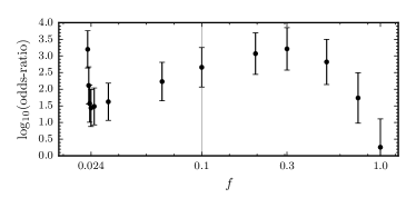
Figure 14: Dependence of the odds-ratio with $f$, the fraction of $P^{\mathrm{ATNF}}$ used to constrain the beam-width priors. The vertical line marks the choice of $f=0.1$ used in our model comparison based on the upper limit given by Lyne & Manchester (1988)

In summary the log-odds-ratio and hence our conclusion is robust to reasonable variations in $f$ from 0.05 to 0.5.

5 Discussion

In this work we are using a data set (provided by Lyne et al. (2010)) on the spin-down and beam-width of B1828-11 to compare models for the observed periodic variations. The two concepts under consideration are free precession and magnetospheric switching. In order to be quantitative, we built signal models for the beam-width and spin-down from these conceptual ideas. Using the spin-down data to create proper, physically motivated priors for the beam-width parameters, we then perform a Bayesian model comparison between the models asking “which model does the beam-width data support?". For the models considered here, the data most strongly supports a precession model with a modified-Gaussian beam geometry allowing for an elliptical beam where the ellipticity has a latitudinal dependence.

To be clear, this does not rule out the switching interpretation since we have not tested an exhaustive set of models—we can only compare between particular models. As an example we could imagine modifying the switching model such that either the switching times, or the magnetospheric states are probabilistic (or a combination of the two). Further we believe there is good grounds to develop models combining the precession and switching interpretation like those discussed in Jones (2012).

In addition to the data considered in this work, a number of high-time-resolution observations of B1828-11 were performed by the Parkes telescope, as discussed in Stairs et al. (2003). This data set shows interesting variability in beam width on short timescales of  O(100) pulses. While the qualitative "noisiness" of the beam-width data is already apparent from the current data-set (eg. see Fig.1), such high-time-resolution data could be very interesting to include in a more detailed future model comparison.

The process of fitting the models to the data and performing posterior predictive checks also provides a mechanism to evaluate the models. For both spin-down models the maximum posterior plots with the data (Figs. 5B and 7B) revealed a systematic failure to fit the second (slightly lower) minima. This suggests new ingredients could be introduced to both models to explain this.

The posteriors for the precession model indicate that B1828-11 is a near-orthogonal rotator and we observe it from close to the equatorial plane. If this is the case, and the two beams of the pulsar are symmetric about the origin, then we expect to see the second beam as an interpulse. Indeed, we discuss further in appendix B how during the precessional cycle we should expect the intensity of this second beam to dominate at certain phases. Since no such interpulse is reported, either the second beam is weaker, or the beams must have a kink of greater than $4.6\degr$ (see appendix B).

In this work we have developed the framework to evaluate models for the variations observed in B1828-11. This is not intended as an exhaustive review of all models, but rather a discussion on the intricacies that arise such as setting up proper and well-motivated priors. This work lays the groundwork for a more exhaustive test of all available models and can also be extended by improvements to the data sources.

Appendix A Procedure for MCMC parameter estimation

The procedure used to simulate the posterior distribution can determine the quality of the estimation. Therefore we will now set out an algorithmic method to ensure the our results are reproducible.

To estimate the posterior given a signal model and prior, we run two MCMC simulations: an initialisation and production. In the following the term walker refers to single chains in the MCMC simulation, the Foreman-Mackey et al. (2013) implementation runs a number of these in parallel for each simulation.

• For the initialisation run, we draw samples from the prior distribution to set the initial parameters for each walker. The simulation therefore has the chance to explore the entire parameter space. After a sufficient number of steps, the walkers will converge to the local maxima in the log-likelihood. By visually inspecting the data we determine the nature of the local maxima: in all cases a single maxima dominated such that, given a sufficient length of simulation, we expect all walkers to converge to this maxima. Alternatively we could have found multiple similarly strong maxima, in this case further analysis would be required. This was not found to be the case for any of the models in this analysis.

• For the second step we set the initial state of 100 walkers by uniformly dispersing them in a small range about the maximum-likelihood found in the previous step. The simulation proceeds from this initial state and we divide the resulting samples equally into two: discarding the first half as a so-called ‘burn-in’, we retain the second half as the production data used to estimate the posterior. The burn-in removes any memory of the artificial initialisation of the walkers at the start of this step.

Having run an MCMC simulation we check that the chains have properly converged (for a discussion on this see Gelman et al. (2013)). The MCMC simulations provide an estimate of the posterior densities for the model parameters. We will also perform ‘posterior predictive checks’ to ensure the posterior is a suitable fit to the data, i.e. we compare the data to the model prediction when the model parameters are set to the values corresponding to the peaks of the posterior probability distributions.

Appendix B Implications for the unobserved beam

The precession model developed here assumes the observer only ever sees one pole of the beam-axis, but in the canonical model we often imagine there is also emission from an opposite magnetic pole. In several pulsars this can be seen as an interpulse $180\degr$ out of phase from the main pulse (Lyne & Manchester, 1988; Maciesiak et al., 2011); these pulsars are generally found to be close to orthogonal rotators. No such interpulse is reported for B1828-11, we will now discuss the implications of this given the precession interpretation.

Let us imagine a scenario where the observer is in the northern (magnetic) hemisphere and label the beam protruding into their hemisphere (which they will see with the greater intensity due to the smaller angular separation) at the start of the thought experiment as the north pole. Then, when $\Theta<\uppi/2$, the north and south pole make angles $\Theta$ and $\uppi-\Theta$ respectively with the fixed angular momentum vector. Now we see that if, during the course of the precessional cycle, $\Theta>\uppi/2$ then the south pole will protrude into the northern hemisphere and the north pole into the southern hemisphere. Provided both poles are identical, but regardless of the details of the beam-geometry, at this time we must expect the observer to see the south pole at greater intensity than the north pole. An example of this is shown in Fig. 15, but note that the observer will see the greatest intensity from the south-pole half a rotation after this instance.

Our posterior distributions inform us that, if the precession interpretation is correct, we are in exactly this situation: $\Theta$ ranges from $85.8\degr$ to $92.3\degr$ over a precessional cycle so we should see the interpulse.

This is readily explained if the south pole is substantially weaker in intensity, or by the one-pole interpretation Manchester & Lyne (1977). Alternatively, it could be that the two beams are not diametrically opposed but are latitudinally ‘kinked’. In the later case we can put a lower bound on the kink angle by requiring that the polar angle of the south pole is always greater than that of the north (see Fig. 15). From our MPE this gives a lower bound of $4.6\degr$ for the polar kink angle. This latitudinal kink can be compared with the longitudinal kink of interpulses observed in other pulsars: often these are not found at exactly $180\degr$, but can deviate by 10’s of degrees (see the separation of interpulses for double-pole interpulses in Table 1. of Maciesiak et al. (2011)). Allowing for such kinks in both beams is a possible extension to the precessional model.

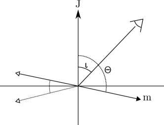
Figure 15: Extension to Fig. 8 adding in the south pole (demarked by a white triangle and solid line) for an instance in which the north pole is in the southern hemisphere. The dotted line with a white arrowhead is the ‘kinked’ beam. For clarity, the north and south poles are shown at times that differ by half a rotation period.

References

- Akgün et al. (2006) Akgün T., Link B., Wasserman I., 2006, MNRAS, 365, 653
- Arzamasskiy et al. (2015) Arzamasskiy L., Philippov A., Tchekhovskoy A., 2015, MNRAS, 453, 3540
- Bailes et al. (1993) Bailes M., Lyne A. G., Shemar S. L., 1993, in Phillips J. A., Thorsett S. E., Kulkarni S. R., eds, Astronomical Society of the Pacific Conference Series Vol. 36, Planets Around Pulsars. pp 19–30
- Cordes (1993) Cordes J., 1993, in Planets around pulsars. pp 43–60, http://adsabs.harvard.edu/full/1993ASPC...36...43C
- Cordes (2013) Cordes J. M., 2013, ApJ, 775, 47
- Davis & Goldstein (1970) Davis L., Goldstein M., 1970, The Astrophysical Journal, 159
- Foreman-Mackey et al. (2013) Foreman-Mackey D., Hogg D. W., Lang D., Goodman J., 2013, PASP, 125, 306
- Foreman-Mackey et al. (2014) Foreman-Mackey D., Price-Whelan A., Ryan G., Emily Smith M., Barbary K., Hogg D. W., Brewer B. J., 2014, triangle.py v0.1.1, doi:10.5281/zenodo.11020, http://dx.doi.org/10.5281/zenodo.11020
- Gelman et al. (2013) Gelman A., Carlin J. B., Stern H. S., Dunson D. B., Vehtari A., Rubin D. B., 2013, Bayesian data analysis. CRC press
- Goggans & Chi (2004) Goggans P. M., Chi Y., 2004, AIP Conference Proceedings, 707, 59
- Goodman & Weare (2010) Goodman J., Weare J., 2010, Communications in applied mathematics and computational science, 5, 65
- Jaynes (2003) Jaynes E. T., 2003, Probability theory: the logic of science. Cambridge university press
- Jeffreys (1998) Jeffreys H., 1998, The theory of probability. OUP Oxford
- Jones (2012) Jones D. I., 2012, MNRAS, 420, 2325
- Jones & Andersson (2001) Jones D. I., Andersson N., 2001, MNRAS, 324, 811
- Landau & Lifshitz (1969) Landau L. D., Lifshitz E. M., 1969, Mechanics. Pergamon press
- Link (2003) Link B., 2003, Physical Review Letters, 91, 101101
- Link & Epstein (2001) Link B., Epstein R. I., 2001, ApJ, 556, 392
- Lyne & Manchester (1988) Lyne A. G., Manchester R. N., 1988, MNRAS, 234, 477
- Lyne et al. (2010) Lyne A., Hobbs G., Kramer M., Stairs I., Stappers B., 2010, Science, 329, 408
- MacKay (2003) MacKay D. J., 2003, Information theory, inference and learning algorithms. Cambridge university press
- Maciesiak et al. (2011) Maciesiak K., Gil J., Ribeiro V. A. R. M., 2011, MNRAS, 414, 1314
- Manchester & Lyne (1977) Manchester R. N., Lyne A. G., 1977, MNRAS, 181, 761
- Manchester et al. (2005) Manchester R. N., Hobbs G. B., Teoh A., Hobbs M., 2005, The Astronomical Journal, 129, 1993
- Narayan & Vivekanand (1983) Narayan R., Vivekanand M., 1983, A&A, 122, 45
- Perera et al. (2015) Perera B. B. P., Stappers B. W., Weltevrede P., Lyne A. G., Bassa C. G., 2015, MNRAS, 446, 1380
- Radhakrishnan & Cooke (1969) Radhakrishnan V., Cooke D. J., 1969, Astrophys. Lett., 3, 225
- Seymour & Lorimer (2013) Seymour A. D., Lorimer D. R., 2013, MNRAS, 428, 983
- Shaham (1977) Shaham J., 1977, ApJ, 214, 251
- Sivia & Skilling (1996) Sivia D. S., Skilling J., 1996, Data analysis: a Bayesian tutorial. Oxford university press
- Stairs et al. (2000) Stairs I., Lyne A., Shemar S., 2000, Nature, 406, 484
- Stairs et al. (2003) Stairs I. H., Athanasiadis D., Kramer M., Lyne A. G., 2003, in Bailes M., Nice D. J., Thorsett S. E., eds, Astronomical Society of the Pacific Conference Series Vol. 302, Radio Pulsars. p. 249 (arXiv:astro-ph/0211005)
- Swendsen & Wang (1986) Swendsen R. H., Wang J.-S., 1986, Phys. Rev. Lett., 57, 2607