Wave phenomena of the Toda lattice with steplike initial data

Abstract.

We give a survey of the long-time asymptotics for the Toda lattice with steplike constant initial data using the nonlinear steepest descent analysis and its extension based on a suitably chosen $g$-function. Analytic formulas for the leading term of the asymptotic solutions of the Toda shock and rarefaction problems (including the case of overlapping background spectra) are given and complemented by numerical simulations. We provide an explicit formula for the modulated solution in terms of Abelian integrals on the underlying hyperelliptic Riemann surface.

1. Introduction

We are interested in the long-time behavior of an infinite particle chain with nonlinear nearest neighbor interactions when the chain is subjected to shock or rarefaction type initial conditions. The continuous spectrum of the underlying Lax operator consists of two intervals which might overlap and their mutual location produces essentially different types of asymptotic solutions. These wave phenomena were first discovered numerically in [11, 12], a rigorous investigation of the limiting behavior as $t\to\infty$ has been carried out so far only for special initial values [5, 13, 18]. This introductory article gives an overview of the new set of results on the Toda shock and rarefaction problems, in particular, we present the leading term of the long-time asymptotic solution for arbitrary steplike constant initial data. The mathematical proof is given in [10] and a forthcoming paper.

Consider the doubly infinite Toda lattice ([16, 17]) in Flaschka’s variables

(1.1) $$\begin{split}\dot{b}(n,t)&=2(a(n,t)^{2}-a(n-1,t)^{2}),\\ \dot{a}(n,t)&=a(n,t)(b(n+1,t)-b(n,t)),\end{split}$$

$(n,t)\in\mathbb{Z}\times\mathbb{R}$, where the dot denotes differentiation with respect to time. We study a steplike initial profile

(1.2) $$\begin{split}&a(n,0)\to a_{\ell},\quad b(n,0)\to b_{\ell},\quad\mbox{as $n\to-\infty$},\\ &a(n,0)\to a_{r}\quad b(n,0)\to b_{r},\quad\mbox{as $n\to+\infty$},\end{split}$$

where the left and right background Jacobi operators with constant coefficients $a_{\ell,r}>0$, $b_{\ell,r}\in\mathbb{R}$,

$$(H_{\ell,r}y)(n)=a_{\ell,r}y(n-1)+b_{\ell,r}y(n)+a_{\ell,r}y(n+1),\quad n\in\mathbb{Z},$$

have spectra in the following general location:

$$\sigma(H_{\ell})\neq\sigma(H_{r}).$$

Each of these spectra consist of one interval and in the literature so far, only background spectra of equal length (that is, when $a_{\ell}=a_{r}$) have been partly investigated. Under this assumption, there are two classical cases, distinguished by the conditions $\inf\sigma(H_{\ell})<\inf\sigma(H_{r})$ (the Toda shock problem) and $\inf\sigma(H_{\ell})>\inf\sigma(H_{r})$ (the Toda rarefaction problem). The Toda shock problem with non-overlapping background spectra was studied by Venakides, Deift, and Oba [18]. This case is depicted in Fig. 1, where the numerically computed solution corresponding to the step $b(n,0)=0$ if $n\geq 0$, $b(n,0)=-3$ if $n<0$, and $a(n,0)\equiv\frac{1}{2}$ is plotted at a frozen time $t=110$ for $500$ plotpoints around the origin. These data correspond to a pure step without solitons. In areas where the functions $n\mapsto a(n,t)$ and $n\mapsto b(n,t)$ seem to be continuous this is due to scaling, since we have plotted a large number of particles, and also due to the $2$-periodicity in space. So one can think of the two lines in the middle region as the even- and odd-numbered particles of the lattice.

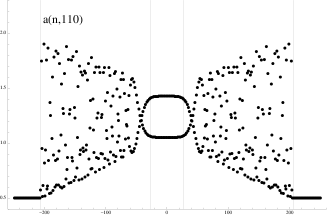
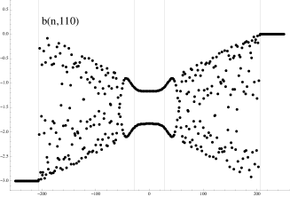
Figure 1. Toda shock problem at $t=110$ with non-overlapping background spectra of equal length, $\sigma(H_{\ell})=[-4,-2]$ and $\sigma(H_{r})=[-1,1]$.

There are five principal regions in the half plane $n/t$ divided by rays $\pm\xi_{cr}$, $\pm\xi_{cr}^{\prime}$, $\xi_{cr}^{\prime}<\xi_{cr}$, with transitional regions around the rays. The points $n_{cr}=\xi_{cr}\times 110$ are plotted as vertical lines to mark the different regions. In the middle region $|\frac{n}{t}|<\xi_{cr}^{\prime}$, the solution can be asymptotically described by a periodic Toda solution of period two, which was the main result of [18]. In the region $\frac{n}{t}>\xi_{cr}$, the solution is asymptotically close to the constant right background solution $(a_{r},b_{r})$, and in the domain $\frac{n}{t}<-\xi_{cr}$, it is close to the left background $(a_{\ell},b_{\ell})$. For the remaining region $\xi_{cr}^{\prime}<|\frac{n}{t}|<\xi_{cr}$, it was conjectured in [18] that the solution is asymptotically close to a modulated single-phase quasi-periodic solution, but despite some follow-up publications ([1, 2, 13]), this problem remained open. We give a precise analytical description of this solution in Sec. 3.1 and [10]. For the transitional regions around $\pm\xi_{cr}$, one can expect the appearance of asymptotic solitons (compare [4]), whereas the transitional regions around $\pm\xi_{cr}^{\prime}$ have not been studied yet from an analytical point of view. Soliton asymptotics in the region $|\frac{n}{t}|>\xi_{cr}$ have been described in [3] using the inverse scattering transform.

As for the Toda rarefaction problem, the only known result is by Deift, Kamvissis, Kriecherbauer, and Zhou [5], who considered non-overlapping background spectra in the case $t\to\infty$ with $n$ fixed, which corresponds to the transitional region around $0$ in Fig. 2. The other regions have not been studied until now, and we present the leading term of the asymptotic solutions in Sec. 3.2. The proof is deferred to a forthcoming paper.

Figure 2. Toda rarefaction problem with non-overlapping background spectra $\sigma(H_{\ell})=[2,4]$ and $\sigma(H_{r})=[-1,1]$.

In this review we allow any possible location for the intervals $\sigma(H_{\ell})$, $\sigma(H_{r})$. First of all, we extend the notion of Toda shock respectively rarefaction to include background spectra of different length, $a_{\ell}\neq a_{r}$. If they overlap, they have to satisfy (in addition to the conditions on the infima of the spectra) the condition $\sup\sigma(H_{\ell})\leq\sup\sigma(H_{r})$ for shock, or $\sup\sigma(H_{r})\leq\sup\sigma(H_{\ell})$ for rarefaction, respectively. Otherwise, if one background spectrum is embedded in the other, $\sigma(H_{\ell})\subset\sigma(H_{r})$ or $\sigma(H_{r})\subset\sigma(H_{\ell})$, it will produce mixed cases with a region where the solution is asymptotically close to a modulated two band Toda lattice solution and a second region where the asymptotic solution is given by a slope as in Fig. 2. These mixed cases are described in Sec. 4.3. Let us mention that the limiting behavior for a flat background $\sigma(H_{\ell})=\sigma(H_{r})$ is well understood by now, see the review article [15] for decaying and [14] for quasi-periodic background operators.

2. The Riemann–Hilbert problem for steplike constant background

Without loss of generality we choose $a_{r}=\frac{1}{2}$, $b_{r}=0$ as the right initial data by shifting and scaling the spectral parameter $\lambda$ in the isospectral problem $H(t)y=\lambda y$. Here $H(t)$ is the Jacobi operator associated with the coefficients $a(t),b(t)$. Suppose that the initial data (1.2) decay to their backgrounds exponentially fast (in the sense of [10]). Denote the spectra of the background operators by

$$I_{\ell}=\sigma(H_{\ell})=[b_{\ell}-2a_{\ell},b_{\ell}+2a_{\ell}],\quad I_{r}=\sigma(H_{r})=[-1,1].$$

The (absolutely) continuous spectrum of $H(t)$ consists of a part $(I_{\ell}\cup I_{r})\setminus(I_{\ell}\cap I_{r})$ of multiplicity one and a part $I_{\ell}\cap I_{r}$ of multiplicity two (if present). We assume for simplicity that $H$ has no eigenvalues, so no solitons are present.

The perturbed solution $(a,b)$ of (1.1), (1.2) can be computed via the inverse scattering transform (IST). The case without step ($H_{\ell}=H_{r}$) is well-known (see [16, 17]); the general steplike case applicable here has been analyzed in [8, 9]. To obtain the long-time asymptotics of this solution we use a modification of IST in the form of a Riemann–Hilbert problem (RHP) on the underlying Riemann surface formed by combining both background spectra. For example, for non-overlapping background spectra the Riemann surface associated with the square root

(2.1) $$P(\lambda)=-\sqrt{(\lambda^{2}-1)((\lambda-b_{\ell})^{2}-4a_{\ell})}$$

is $2$-sheeted over the complex plane where one changes sheets along the segments $I_{\ell}$ and $I_{r}$. The square root plays the role of the projection onto the complex plane. A point on the Riemann surface is denoted by $p=(\lambda,\pm)$, $\lambda\in\mathbb{C}$, with $p=(\infty,\pm)=\infty_{\pm}$. Let $\Sigma_{\ell}$ and $\Sigma_{r}$ be clockwise oriented contours around the cuts $I_{\ell}$ and $I_{r}$ on the upper sheet of the Riemann surface. The asymptotic solution can be read off from a vector-valued function $m$ defined on the upper sheet using the right scattering data,

$$m(p,n,t)=\begin{pmatrix}T(p,t)\psi_{\ell}(p,n,t)z^{n}(p),&\psi(p,n,t)z^{-n}(p)\end{pmatrix}.$$

Here $T(p,t)$ is the right transmission coefficient and $\psi$, $\psi_{\ell}$ are the Jost solutions of $H(t)y=\lambda y$ which asymptotically look like the free solutions of the background operators $H_{r}$ and $H_{\ell}$. The function $z(p)=\lambda-\sqrt{\lambda^{2}-1}$, $|z(p)|<1$, is the Joukovski transform of the spectral parameter $\lambda$. We extend $m$ to the lower sheet by the symmetry condition

$$m(p^{*})=m(p)\begin{pmatrix}0&1\\ 1&0\end{pmatrix},$$

where $p^{*}=(\lambda,-)$ is the flip image of $p=(\lambda,+)$ on the lower sheet. With this extension, the scattering relations between the Jost solutions translate to jump conditions for $m$ along $\Sigma_{\ell}$ and $\Sigma_{r}$. To formulate them, let $m_{+}(p)$ denote the limit of $m(\zeta)$ as $\zeta\to p$ from the positive side of $\Sigma$; the positive side is the one which lies to the left of $\Sigma$ as one traverses $\Sigma$ in the direction of its orientation. Similarly, $m_{-}(p)$ denotes the limit from the negative side of $\Sigma$. Then $m$ is holomorphic away from $\Sigma_{\ell}\cup\Sigma_{r}$ with jump condition $m_{+}(p,n,t)=m_{-}(p,n,t)v(p,n,t)$ and jump matrix

$$v(p,n,t)=\left\{\begin{array}[]{ll}\begin{pmatrix}1-|R(p)|^{2}&-\overline{R(p)}\mathrm{e}^{-2t\Phi(p,n/t)}\\[2.84526pt] R(p)\mathrm{e}^{2t\Phi(p,n/t)}&1\end{pmatrix},&\quad p\in\Sigma,\\[14.22636pt] \begin{pmatrix}0&-\overline{R(p)}\mathrm{e}^{-2t\Phi(p,n/t)}\\[2.84526pt] R(p)\mathrm{e}^{2t\Phi(p,n/t)}&1\end{pmatrix},&\quad p\in\Sigma_{r}\setminus\Sigma,\\[14.22636pt] \begin{pmatrix}\chi(p)\mathrm{e}^{t(\Phi_{+}(p,n/t)-\Phi_{-}(p,n/t))}&1\\[2.84526pt] 1&0\end{pmatrix},&\quad p\in\Sigma_{\ell}\setminus\Sigma,\end{array}\right.$$

where $\Sigma$ is the clockwise oriented contour around the spectrum of multiplicity two $I_{\ell}\cap I_{r}$ (if present). The function $m=(m_{1},m_{2})$ has positive limiting values as $p\to\infty_{\pm}$ satisfying $m_{1}(\infty_{\pm})m_{2}(\infty_{\pm})=1$. In the matrix elements of the jumps, $R(p)$ is the right reflection coefficient at $t=0$ and $\chi$ is the limit from the upper sheet $\Pi_{U}$ of the right transmission coefficient $T(x)$ at $t=0$,

$$\chi(p)=-\lim_{x\in\Pi_{U}\to p\in\Sigma_{\ell}}\sqrt{\frac{(x-b_{\ell})^{2}-4a_{\ell}^{2}}{x^{2}-1}}\ |T(x)|^{2}.$$

The phase function $\Phi$ is given on the closure of the upper sheet by

$$\Phi(p,n/t)=\frac{1}{2}\big{(}z(p)-z^{-1}(p)\big{)}+\frac{n}{t}\log z(p)$$

and continued as an odd function on the lower sheet with a jump on $\Sigma_{\ell}\setminus\Sigma$. The expansion of the first component of $m$ as $p\to\infty_{+}$ yields the precise connection to $a,b$,

$$m_{1}(p,n,t)=\prod_{j=n}^{\infty}2a(j,t)\Big{(}1+\frac{1}{\lambda}\ \sum_{m=n}^{\infty}b(m,t)\Big{)}+O\Big{(}\frac{1}{\lambda^{2}}\Big{)}.$$

If $H$ has eigenvalues, then $m$ is meromorphic away from $\Sigma_{\ell}\cup\Sigma_{r}$ with pole conditions

$$\operatorname{Res}_{p_{j}}m(p)=\lim_{p\to p_{j}}m(p)\begin{pmatrix}0&0\\ A_{j}&0\end{pmatrix},\quad\operatorname{Res}_{p_{j}^{*}}m(p)=\lim_{p\to p_{j}^{*}}m(p)\begin{pmatrix}0&A_{j}\\ 0&0\end{pmatrix},$$

where $p_{j}$ and $p_{j}^{*}$ denote the eigenvalue $\lambda_{j}$ on the upper and lower sheet and

$$A_{j}=\sqrt{p_{j}^{2}-1}\beta_{j}\mathrm{e}^{2t\Phi(p_{j},n,t)}.$$

Here $\beta_{j}$, $j=1,\dots,N$, are the right norming constants at time $t=0$.

One tries to find a factorization of the jump matrices in order to transform the initial RHP to an equivalent RHP with jump matrices close to constant matrices on contours for large $t$, which can be solved explicitly. The asymptotic solution for $a,b$ can then be read off using the expansion of $m$ at $\infty_{+}$. The crucial step in the nonlinear stationary phase method [7] is to reduce the given RHP to one or more RHPs localized at stationary phase points, which can be analyzed and controlled individually. However, the steplike case requires an extension of this method based on a suitably chosen $g$-function as first introduced in [6] which replaces the phase function $\Phi$. Since the jump contour of the limiting RHP depends on the slow variable $\xi=\frac{n}{t}$, this determines a special choice for the $g$-function. The expected asymptotic solution is finite band and corresponds to a modified Riemann surface which is ”truncated” with respect to the initial Riemann surface and moves with $\xi$. So we choose the $g$-function as a sum of Abel integrals such that the line $\mathop{\mathrm{Re}}g=0$ passes through the moving end of the truncated Riemann surface and such that the $g$-function approximates the phase function at infinity up to an additive constant. Then this $g$-function transforms the jump matrices in a way that allows us to factorize them and to get asymptotically constant matrices on contours. In the case of the Toda rarefaction problem with overlapping background spectra, the modified Riemann surface corresponds to just one interval, and we describe this simple dependence of the asymptotic solution in Sec. 4.2 in more detail.

3. Asymptotic solution for non-overlapping background spectra

3.1. Toda shock problem

Assume that the background spectra are in shock position and do not overlap, $b_{\ell}+2a_{\ell}<-1$. Fig. 3 depicts the numerically computed solution corresponding to the step $(a(n,0),b(n,0))=(\frac{1}{2},0)$ if $n\geq 0$ and $(a(n,0),b(n,0))=(a_{\ell},b_{\ell})$ if $n<0$ at $t=140$ with non-overlapping background spectra ($a_{\ell}=0.4$, $b_{\ell}=-2$).

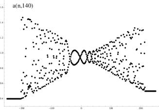
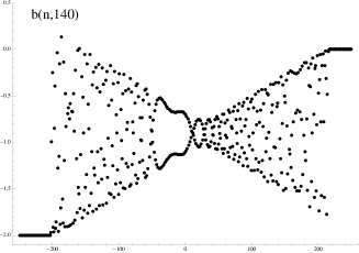
Figure 3. Numerically computed solution $a$ and $b$ of the Toda shock problem with $\sigma(H_{\ell})=[-2.8,-1.2]$ and $\sigma(H_{r})=[-1,1]$.

One can distinuish five principal regions in the half plane $n/t$ divided by rays $n_{cr}/t=\xi_{cr}$, where $\xi_{cr}$ is one of four critical points satisfying $\xi_{\ell}<\xi_{\ell}^{\prime}<\xi_{r}^{\prime}<\xi_{r}$ (compare also Fig. 5 at a later time $t=270$, where $n_{cr}=\xi_{cr}\times 270$ are plotted as vertical lines to mark the different regions). Analyzing the curve $\mathop{\mathrm{Re}}\Phi(\lambda,\xi)=0$ yields that the critical point $\xi_{r}$ is the solution of

(3.1) $$\int_{\inf I_{\ell}}^{-1}\frac{x+\xi_{r}}{\sqrt{x^{2}-1}}dx=0,\quad\xi_{r}=\frac{\sqrt{(-b_{\ell}+2a_{\ell})^{2}-1}}{\log(-b_{\ell}+2a_{\ell}+\sqrt{(-b_{\ell}+2a_{\ell})^{2}-1})},$$

the remaining points $\xi_{cr}$ are given in [10]. In the region $\xi>\xi_{r}$, the solution is asymptotically close to the constant right background solution $(\frac{1}{2},0)$, and in the domain $\xi<\xi_{\ell}$, it is close to the left background $(a_{\ell},b_{\ell})$.

In the domain $\xi_{r}^{\prime}<\xi<\xi_{r}$, we find a monotonic smooth function $\gamma(\xi)\in I_{\ell}$ such that $\gamma(\xi_{r}^{\prime})=\sup I_{\ell}$, $\gamma(\xi_{r})=\inf I_{\ell}$. When the parameter $\xi$ starts to decay from the point $\xi_{r}$, the point $\gamma(\xi)$ “opens” a band $[\inf I_{\ell},\gamma(\xi)]=I_{\ell}(\xi)$ (the Whitham zone). The intervals $I_{\ell}(\xi)$ and $I_{r}$ can be treated as the bands of a (slowly modulated) finite band solution of the Toda lattice, which turns out to give the leading asymptotic term of our solution with respect to large $t$. This finite band solution is modulated by the gradual lengthening of the lower band and defined uniquely by its initial divisor. We compute this divisor precisely via the values of the right transmission coefficient on the interval $I_{\ell}(\xi)$. Thus, in a vicinity of any ray $n/t=\xi$ the solution of (1.1)–(1.2) is asymptotically two band. This asymptotic term also can be treated as a function of $n$, $t$, and $\frac{n}{t}$ in the whole domain $t(\xi_{r}^{\prime}+\varepsilon)<n<t(\xi_{r}-\varepsilon)$. To obtain analytical formulas, one shows that for any $\xi\in(\xi_{r}^{\prime},\xi_{r})$ there exist $\gamma(\xi)\in I_{\ell}$ and $\mu(\xi)\in(\gamma(\xi),-1)$ satisfying

$$2a_{\ell}-b_{\ell}+\gamma(\xi)+2\mu(\xi)=-2\xi,\quad\int_{\gamma(\xi)}^{-1}\frac{\big{(}\lambda-\mu(\xi)\big{)}\big{(}\lambda-\gamma(\xi)\big{)}}{P(\lambda,\gamma)}d\lambda=0,$$

where

$$P(\lambda,\gamma)=-\sqrt{(\lambda^{2}-1)(\lambda-b_{\ell}+2a_{\ell})(\lambda-\gamma(\xi))}.$$

Then the $g$-function with the desired properties to transform the jump matrices is given by (see [10, Sec. 3])

$$g(p,\xi)=\int_{1}^{p}\frac{\big{(}\lambda-\mu(\xi)\big{)}\big{(}\lambda-\gamma(\xi)\big{)}}{P(\lambda,\gamma)}d\lambda.$$

Associated with the square root $P(\lambda,\gamma)$ is the ”truncated” Riemann surface $\mathbb{M}(\xi)$. Let $\zeta$ be the normalized holomorphic Abel differential (which depends on $\xi$) on $\mathbb{M}(\xi)$. The divisor $\rho(\xi)$ of the two band solution under consideration is uniquely defined by the following Jacobi inversion problem

$$\int_{\inf I_{\ell}}^{\rho(\xi)}\zeta=\int_{\inf I_{\ell}}^{\gamma(\xi)}\zeta-\frac{\mathrm{i}}{\pi}\int_{\inf I_{\ell}}^{\gamma(\xi)}\log|\chi|\zeta+\int_{\infty_{-}}^{\infty_{+}}\zeta.$$

Introduce the function

$$\underline{z}(n,t)=\int_{\inf I_{\ell}}^{\infty_{+}}\zeta-\int_{\inf I_{\ell}}^{\rho(\xi)}\zeta-n\int_{\infty_{-}}^{\infty_{+}}\zeta+\frac{t}{\pi\mathrm{i}}\int_{\inf I_{\ell}}^{\gamma(\xi)}\Omega_{0}-\Xi(\xi),$$

where $\Xi(\xi)$ is the Riemann constant and $\Omega_{0}$ is the normalized Abel differential of the second kind on $\mathbb{M}(\xi)$ with second order poles at $\infty_{-}$ and $\infty_{+}$. Let

$$\theta(v)=\sum_{m\in\mathbb{Z}}\exp\big{(}\pi\mathrm{i}m^{2}\tau+2\pi\mathrm{i}mv\big{)}$$

be the Riemann theta function of the surface $\mathbb{M}(\xi)$ and set

(3.2) $$\begin{split}b_{q}(n,t,\xi)&=\tilde{b}+\frac{1}{\Gamma}\,\frac{\partial}{\partial w}\log\left(\frac{\theta\big{(}\underline{z}(n-1,t)+w\big{)}}{\theta\big{(}\underline{z}(n,t)+w\big{)}}\right)\Big{|}_{w=0},\\ a^{2}_{q}(n,t,\xi)&=\tilde{a}^{2}\,\frac{\theta(\underline{z}(n-1,t))\theta(\underline{z}(n+1,t))}{\theta^{2}(\underline{z}(n,t))},\end{split}$$

which describe a classical two band Toda lattice motion corresponding to the bands $I_{\ell}(\xi)$ and $I_{r}$ with initial divisor $\rho(\xi)$ (compare [16, Sec. 9]). Here $\tilde{a}$, $\tilde{b}$ are the averages and $\Gamma=\int_{\mathfrak{a}}\zeta$. Then for $\xi\in(\xi_{r}^{\prime},\xi_{r})$ in the vicinity of any ray $n=\xi t$, the solution has the asymptotic behavior as $t\to+\infty$

$$a^{2}(n,t)=a^{2}_{q}(n,t,\xi)+o(1),\quad b(n,t)=b_{q}(n,t,\xi)+o(1).$$

A numerical comparison between the solution and the asymptotic formula is given in Fig. 4 (due to [10]). There we computed the two band Toda solution (blue) precisely via (3.2) for the pure step initial data and plotted it against the numerical solution (black) with the same initial data.

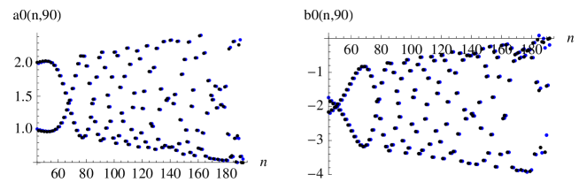
Figure 4. Comparison between the solution (black) and the asymptotic formula (blue) in the region $\xi_{r}^{\prime}<\xi<\xi_{r}$.

In the gap domain $\xi_{\ell}^{\prime}<\xi<\xi_{r}^{\prime}$, the asymptotic of the solution of (1.1)–(1.2) is described by a two band Toda lattice solution connected with one and the same intervals $I_{\ell}$ and $I_{r}$ and the initial divisor $\rho$ (or shift of the phase) defined by

$$\int_{\inf I_{\ell}}^{\rho}\zeta=\int_{\inf I_{\ell}}^{\sup I_{\ell}}\zeta-\frac{\mathrm{i}}{2\pi}\int_{\Sigma_{\ell}}\log|\chi|\zeta+\int_{\infty_{-}}^{\infty_{+}}\zeta$$

does not depend on the slow variable $\xi$. Here $\zeta$ is the normalized holomorphic Abel differential on the initial Riemann surface associated with $P(\lambda)$ (cf. (2.1)). Then the solution of (1.1)–(1.2) is asymptotically close to $a_{q}(n,t),b_{q}(n,t)$ constructed as above, but independent of $\xi$, as $t\to\infty$ uniformly in $n/t\in[\xi_{\ell}^{\prime}+\varepsilon,\xi_{r}^{\prime}-\varepsilon]$. For the comparison with the numerical solution in Fig. 5, we expressed $a_{q},b_{q}$ in terms of Jacobi’s elliptic functions (cf. [16, Sec. 9.3]). Note that if solitons were present in the gap between the background spectra, new two band solutions associated with $I_{\ell}$ and $I_{r}$ would appear to the left and to the right of each soliton, differing by a phase shift (see [10]). If the background spectra are of equal length, $a_{\ell}=\frac{1}{2}$, the solution $a_{q},b_{q}$ is periodic (Fig. 1 and [18]).

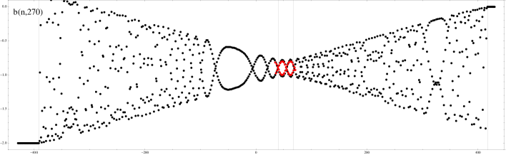
Figure 5. Comparison between the $b$ coefficient (black) of Fig. 3 at time $t=270$ and the asymptotic formula (red) in the region $\xi_{\ell}^{\prime}<\xi<\xi_{r}^{\prime}$.

In the second Whitham zone $\xi_{\ell}<\xi<\xi_{\ell}^{\prime}$, there is a monotonic smooth function $\gamma_{\ell}(\xi)\in I_{r}$ with $\gamma_{\ell}(\xi_{\ell})=\sup I_{r}$, $\gamma_{\ell}(\xi_{\ell}^{\prime})=\inf I_{r}$. The modulated finite band asymptotic here is local along the ray and defined by the intervals $I_{\ell}$, $[\gamma_{\ell}(\xi),\sup I_{r}]$, and an initial divisor.

3.2. Toda rarefaction problem

Consider the rarefaction problem without overlap of the background spectra, so let $\sup I_{r}=1<\inf I_{\ell}$.

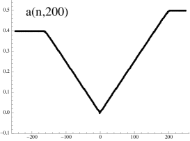
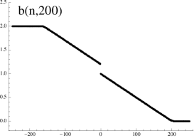
Figure 6. Toda rarefaction problem with non-overlapping background spectra $\sigma(H_{\ell})=[1.2,2.8]$, $\sigma(H_{r})=[-1,1]$; $a_{\ell}=0.4$, $b_{\ell}=2$, $a_{r}=\frac{1}{2}$, $b_{r}=0$.

As illustrated in Fig. 6, the $n/t$ plane splits into four main regions. In the domain $\xi>1$, the solution is asymptotically close to the constant right background solution $(\frac{1}{2},0)$ and in the domain $\xi<-2a_{\ell}$, it is close to the left background solution. For $\xi\in(0,1)$, the solution is asymptotically close to

(3.3) $$a^{2}(n,t)=\left(\frac{n}{2t}\right)^{2}+o(1),\quad b(n,t)=1-\frac{n}{t}+o(1).$$

In the domain $\xi\in(-2a_{\ell},0)$,

(3.4) $$a^{2}(n,t)=\left(\frac{n}{2t}\right)^{2}+o(1),\quad b(n,t)=b_{\ell}-2a_{\ell}-\frac{n}{t}+o(1).$$

The proof of these asymptotics will be provided in a forthcoming paper.

4. Asymptotic solution for overlapping background spectra

In this section we assume that the background spectra $I_{\ell}$ and $I_{r}$ overlap, which means that the Jacobi operator $H(t)$ has a nonempty spectrum of multiplicity two. The asymptotic solution on the region corresponding to this spectrum is given by the constant solution associated with the interval $[b_{\ell}-2a_{\ell},1]$ plus a dispersive tail which decays like $t^{-1/2}$,

(4.1) $$\begin{split}a^{2}(n,t)&=\big{(}(1-b_{\ell}+2a_{\ell})/4\big{)}^{2}+\mbox{oscillation},\\ b(n,t)&=(1+b_{\ell})/2-a_{\ell}+\mbox{oscillation}.\end{split}$$

The oscillatory tail is in agreement with the decaying case [15]. In particular, the asymptotic (4.1) holds true for any type of overlap of $I_{\ell}$ and $I_{r}$.

4.1. Toda shock problem with dispersive tail

Let the background spectra overlap such that $\inf I_{\ell}<-1<\sup I_{\ell}<1$. Then the $n/t$ plane splits into five different regions with boundary points

$$\xi_{\ell}<\frac{1-b_{\ell}-6a_{\ell}}{2}<\frac{b_{\ell}-2a_{\ell}+3}{2}<\xi_{r},$$

where $\xi_{r}$ and $\xi_{\ell}$ are the same as in Sec. 3.1. The boundary values are plotted in Fig. 7 as vertical lines. On the right Whitham zone, $(b_{\ell}-2a_{\ell}+3)/2<\xi<\xi_{r}$, the function $\gamma(\xi)\in[\inf I_{\ell},-1]$ exists and the asymptotic solution is the two band Toda lattice solution $a_{q}^{2},b_{q}$ with initial divisor $\rho(\xi)$ and bands $[\inf I_{\ell},\gamma(\xi)]$ and $I_{r}$ of Sec. 3.1. In the middle region corresponding to the spectrum of multiplicity two, the asymptotic solution is given by (4.1) which we illustrate by plotting the constant term of (4.1) as a horizontal line. This line is at $1.25$ for $a(n,90)$ and at $-1.5$ for $b(n,90)$. On the left Whitham zone, there exists a monotonic smooth function $\gamma_{\ell}(\xi)\in[\max I_{\ell},1]$ and the modulated two band Toda lattice asymptotic here is defined by the intervals $I_{\ell}$ and $[\gamma_{\ell}(\xi),1]$, and an initial divisor as before.

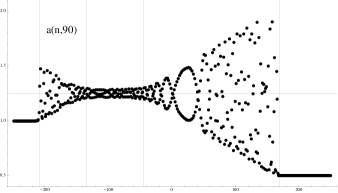
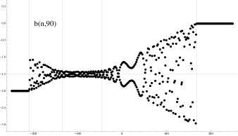
Figure 7. Toda shock with overlapping background spectra $\sigma(H_{\ell})=[-4,0]$ and $\sigma(H_{r})=[-1,1]$; $a_{\ell}=1$, $b_{\ell}=-2$.

4.2. Toda rarefaction problem with dispersive tail

Let the background spectra overlap such that $-1<\inf I_{\ell}<1<\sup I_{\ell}$. Then the $n/t$ plane splits into five regions with boundary points

$$-2a_{\ell}<\frac{b_{\ell}-2a_{\ell}-1}{2}<\frac{1-b_{\ell}+2a_{\ell}}{2}<1.$$

In Fig. 8, the slopes correspond to the spectra of multiplicity one, while the oscillating part is due to the spectrum of multiplicity two.

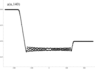
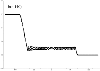
Figure 8. Toda rarefaction with overlapping background spectra $\sigma(H_{\ell})=[-0.9,1.5]$ and $\sigma(H_{r})=[-1,1]$; $a_{\ell}=0.6$, $b_{\ell}=0.3$.

For this problem the underlying Riemann surface of the $g$-function consists of just one interval, which continuously transforms from $I_{r}$ to $I_{\ell}$ as $\xi$ decreases from $+\infty$ to $-\infty$ and determines the leading term of the asymptotic solution, so let us describe this situation in more detail. The difficulty is to find the correct $g$-function which replaces the phase function $\Phi$ in the RHP. The $g$-function differs for each region with matching definitions at the respective boundary points. Let $\eta(\xi)$ be the point where the curve $\mathop{\mathrm{Re}}g=0$ crosses the real axis. As $\xi$ decreases, $\eta(\xi)$ increases from $-\infty$ to $+\infty$. For $\xi>1$, the Riemann surface corresponds to $I_{r}$ and the solution is asymptotically close to $(\frac{1}{2},0)$. When $\xi$ starts to decay from $1$, the point $\eta(\xi)=1-2\xi$ truncates $I_{r}$ to $[\eta(\xi),1]$ and the solution is asymptotically close to (3.3). When $\xi$ passes the second boundary point $(1-b_{\ell}+2a_{\ell})/2$, the point $\eta(\xi)$ passes $\inf I_{\ell}$ and the Riemann surface corresponds to $[\inf I_{\ell},1]$. The asymptotic solution is given by the constant solution with dispersive tail (4.1). When $\xi$ is at the third boundary point, $\eta(\xi)$ crosses $1$, and the interval starts to enlarge, $[\inf I_{\ell},\eta(\xi)]$, with $\eta(\xi)=b_{\ell}-2a_{\ell}-2\xi$. The solution is asymptotically close to (3.4). When $\xi$ passes $-2a_{\ell}$, $\eta(\xi)$ is at $\sup I_{\ell}$, and the Riemann surface corresponds to $I_{\ell}$, so the asymptotic solution is $(a_{\ell},b_{\ell})$.

4.3. Mixed cases of embedded background spectra

There are two cases to consider, either $I_{r}$ is embedded in $I_{\ell}$ or $I_{\ell}$ is a subset of $I_{r}$.

Case 1: Let $I_{r}\subset I_{\ell}$ (compare Fig. 9). The boundary points of the different regions are given by

$$-2a_{\ell}<\frac{b_{\ell}-2a_{\ell}-1}{2}<\frac{b_{\ell}-2a_{\ell}+3}{2}<\xi_{r},$$

with $\xi_{r}$ as in (3.1). The two band solution of the Whitham zone is defined by the intervals $[\inf I_{\ell},\gamma(\xi)]$ and $[-1,\sup I_{\ell}]$ with divisor $\rho_{e}(\xi)$, where the normalized holomorphic Abel differential used in the definition of $\rho_{e}(\xi)$ involves the square root $-\sqrt{(\lambda+1)((\lambda-b_{\ell})^{2}-4a_{\ell}^{2})(\lambda-\gamma)}$. In the middle region, the asymptotic is given by the constant solution (4.1) with dispersive tail and in the region $-2a_{\ell}<\xi<\frac{b_{\ell}-2a_{\ell}-1}{2}$, it is given by (3.4). For $\xi<-2a_{\ell}$ and $\xi>\xi_{r}$, the particles are close to the unperturbed lattice.

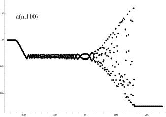
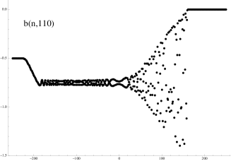
Figure 9. Mixed case with background spectrum $\sigma(H_{r})=[-1,1]$ embedded in $\sigma(H_{\ell})=[-2.5,1.5]$; $a_{\ell}=1$, $b_{\ell}=-\frac{1}{2}$.

Case 2: Let $I_{\ell}\subset I_{r}$. The boundary points of the different regions in Fig. 10 are given by

$$\xi_{cr}<\frac{1-b_{\ell}}{2}-3a_{\ell}<\frac{1-b_{\ell}}{2}+a_{\ell}<1,$$

where $\xi_{cr}$ is the solution of

$$\int_{\sup I_{\ell}}^{1}\frac{x-b_{\ell}+\xi_{cr}}{\sqrt{((x-b_{\ell})^{2}-4a_{\ell}^{2})}}dx=0.$$

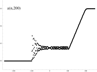
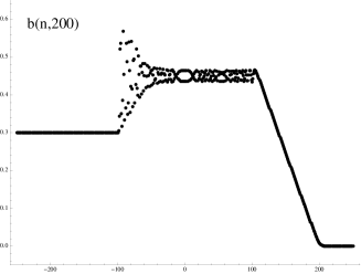
Figure 10. Mixed case with background spectrum $\sigma(H_{\ell})=[-0.1,0.7]$ embedded in $\sigma(H_{r})=[-1,1]$; $a_{\ell}=0.2$, $b_{\ell}=0.3$.

For $\xi>1$, the solution is asymptotically close to the right background solution, the interval corresponding to the underlying Riemann surface of the $g$-function is $I_{r}$. When $\eta(\xi)$ passes $-1$, $I_{r}$ is shortened to $[\eta(\xi),1]$ and the asymptotic solution is (3.3) until $\eta(\xi)$ passes $\inf I_{\ell}$. Then the Riemann surface corresponds to $[\inf I_{\ell},1]$ with asymptotic solution (4.1) until $\eta(\xi)$ crosses $\sup I_{\ell}$, at which point a gap opens and the surface corresponds to $I_{\ell}\cup{[\eta(\xi),1]}$. Hence for $\xi\in(\xi_{cr},\frac{1-b_{\ell}}{2}-3a_{\ell})$, the asymptotic solution is the two band Toda lattice solution associated with the bands $I_{\ell}$, $[\eta(\xi),1]$, and an initial divisor. Here $\eta(\xi)=1+2b_{\ell}-2\xi-2\mu(\xi)$ and the function $\mu(\xi)\in(\sup I_{\ell},\eta(\xi))$ is the solution of

$$\int_{\sup I_{\ell}}^{\eta(\xi)}\frac{(x-\mu(\xi))\sqrt{x-\eta(\xi)}}{\sqrt{((x-b_{\ell})^{2}-4a_{\ell}^{2})(x-1)}}dx=0.$$

When $\eta(\xi)$ crosses $1$ (as $\xi$ crosses $\xi_{cr}$), we are left with $I_{\ell}$.

Acknowledgment. The author is indebted to Iryna Egorova and the referee for constructive remarks. This work was supported by the Austrian Science Fund (FWF) under Grant No. V120.

References

- [1] A. M. Bloch and Y. Kodama, The Whitham equation and shocks in the Toda lattice, Proceedings of the NATO Advanced Study Workshop on Singular Limits of Dispersive Waves held in Lyons, July 1991, Plenum Press, New York, 1994.
- [2] A. M. Bloch and Y. Kodama, Dispersive regularization of the Whitham equation for the Toda lattice, SIAM J. Appl. Math. 52, 909–928 (1992).
- [3] A. Boutet de Monvel and I. Egorova, The Toda lattice with step-like initial data. Soliton asymptotics, Inverse Problems 16, No.4, 955–977 (2000).
- [4] A. Boutet de Monvel, I. Egorova, and E. Khruslov, Soliton asymptotics of the Cauchy problem solution for the Toda lattice, Inverse Problems 13, No.2, 223–237 (1997).
- [5] P. Deift, S. Kamvissis, T. Kriecherbauer, and X. Zhou, The Toda rarefaction problem, Comm. Pure Appl. Math. 49, No.1, 35–83 (1996).
- [6] P. Deift, S. Venakides, and X. Zhou, The collisionless shock region for the long time behavior of solutions of the KdV equation, Comm. Pure and Appl. Math. 47, 199–206 (1994).
- [7] P. Deift and X. Zhou, A steepest descent method for oscillatory Riemann–Hilbert problems, Ann. of Math. (2) 137, 295–368 (1993).
- [8] I. Egorova, J. Michor, and G. Teschl, Scattering theory for Jacobi operators with general steplike quasi-periodic background, Zh. Mat. Fiz. Anal. Geom. 4, No.1, 33–62 (2008).
- [9] I. Egorova, J. Michor, and G. Teschl, Inverse scattering transform for the Toda hierarchy with steplike finite-gap backgrounds, J. Math. Physics 50, 103522 (2009).
- [10] I. Egorova, J. Michor, and G. Teschl, Long-time asymptotics for the Toda shock problem: non-overlapping spectra, arXiv:1406.0720.
- [11] B. L. Holian and G. K. Straub, Molecular dynamics of shock waves in one-dimensional chains, Phys. Rev. B 18, 1593–1608 (1978).
- [12] B. L. Holian, H. Flaschka, and D. W. McLaughlin, Shock waves in the Toda lattice: Analysis, Phys. Rev. A 24, 2595–2623 (1981).
- [13] S. Kamvissis, On the Toda shock problem, Physica D 65, 242-266 (1993).
- [14] S. Kamvissis and G. Teschl, Long-time asymptotics of the periodic Toda lattice under short-range perturbations, J. Math. Phys. 53, No.7, 073706 (2012).
- [15] H. Krüger and G. Teschl, Long-time asymptotics of the Toda lattice for decaying initial data revisited, Rev. Math. Phys. 21, 61–109 (2009).
- [16] G. Teschl, Jacobi Operators and Completely Integrable Nonlinear Lattices, Math. Surv. and Mon. 72, Amer. Math. Soc., Rhode Island, 2000.
- [17] M. Toda, Theory of Nonlinear Lattices, 2nd enl. ed., Springer, Berlin, 1989.
- [18] S. Venakides, P. Deift, and R. Oba, The Toda shock problem, Comm. Pure Appl. Math. 44, No.8-9, 1171–1242 (1991).