Combustion waves in hydraulically resistant porous media in a special parameter regime

Abstract.

In this paper we study the stability of fronts in a reduction of a well-known PDE system that is used to model the combustion in hydraulically resistant porous media. More precisely, we consider the original PDE system under the assumption that one of the parameters of the model, the Lewis number, is chosen in a specific way and with initial conditions of a specific form. For a class of initial conditions, then the number of unknown functions is reduced from three to two. For the reduced system, the existence of combustion fronts follows from the existence results for the original system. The stability of these fronts is studied here by a combination of energy estimates and numerical Evans function computations and nonlinear analysis when applicable. We then lift the restriction on the initial conditions and show that the stability results obtained for the reduced system extend to the fronts in the full system considered for that specific value of the Lewis number. The fronts that we investigate are proved to be either absolutely unstable or convectively unstable on the nonlinear level.

^a ;

^b ,

AMS Classification: 35K57, 35B32, 35B36, 80A25, 35B40.

1. Introduction

Sivashinsky and his collaborators in [1] proposed a model describing combustion in inert porous media under condition of high hydraulic resistance,

(1) $$\begin{split}T_{t}-(1-\gamma^{-1})P_{t}&=\epsilon T_{xx}+YF(T),\\ P_{t}-T_{t}&=P_{xx},\\ Y_{t}&=\epsilon{\rm{Le}}^{-1}Y_{xx}-\gamma YF(T),\end{split}$$

where $Y$ is the scaled concentration of the reactant in the reaction zone, $P$ is the pressure, and $T$ is the temperature. The specific heat ratio $\gamma>1$, the Lewis number ${\rm{Le}}>0$, and the ratio of pressure and molecular diffusivities $\epsilon>0$ are physical characteristics of the fuel. The reaction rate $YF(T)$ may or may not have an ignition cut-off, that is, $F(T)=0$ on an interval $[0,T_{ign}]$ and $F(T)>0$ and increasing for $T>T_{ign}$. For $F(T)$ Lipschitz continuity is assumed everywhere, except at the ignition temperature $T=T_{ign}$. Papers [1, 2, 3] contain detailed explanations and the deduction of this system.

In [4] it is suggested to considered this system with initial conditions

$$T(0,x)=T_{0}(x),\quad Y(0,x)=1,\quad P(0,x)=0.$$

It is also assumed that $\epsilon$ is significantly smaller than other parameters, therefore a simplification of (1) is offered in the literature which is obtained by setting $\epsilon=0$,

(2) $$\begin{split}T_{t}-(1-\gamma^{-1})P_{t}&=YF(T),\\ P_{t}-T_{t}&=P_{xx},\\ Y_{t}&=-\gamma YF(T).\end{split}$$

We point out that the terms $\epsilon T_{xx}$ and $\epsilon{\rm Le}^{-1}Y_{xx}$ in (1) are singular perturbations, so results obtained for the system (2) should be dealt with caution, as singularly perturbed systems in general may support a behavior significantly different than one observed in the limiting system.

This paper is devoted to the study of the stability of traveling fronts in the system (1). Traveling fronts are solutions of the underlying PDE (1) that have a form $T(x,t)=T(\xi)$, $P(x,t)=P(\xi)$, $Y(x,t)=Y(\xi)$, with $\xi=x-ct$, where $c$ is the a priori unknown front speed, and that asymptotically connect distinct equilibria at $\pm\infty$. These solutions are sought as solutions of the traveling wave ODEs

$$-cT^{\prime}+c(1-\gamma^{-1})P^{\prime} = \epsilon T^{\prime\prime}+YF(T),$$

(3) $$P^{\prime\prime} = c(T^{\prime}-P^{\prime}),$$

$$cY^{\prime}+\epsilon Y^{\prime\prime} = \gamma YF(T),$$

that satisfy boundary-like conditions at $\pm\infty$ which we describe below.

Generally speaking, the equilibria of the system (1) are states where $YF(T)=0$, so they can be described as the states where there is no fuel $Y=0$, or as the cold states $T<T_{ign}$. From physical considerations two of the equilibria are of interest, the completely burnt state $P=1$, $T=1$, $Y=0$, and the unburnt state where all of the fuel is present $T=0$, $P=0$, $Y=1$. So we consider the system (1) together with the boundary conditions

$$\begin{split}P(-\infty)=1,\quad T(-\infty)=1,\quad Y(-\infty)=0,\\ T(+\infty)=0,\quad P(+\infty)=0,\quad Y(+\infty)=1.\end{split}$$

The existence and uniqueness of fronts in the system (2) has already been established in [6], under the assumption on the parameters $0<T_{ign}<1-\gamma^{-1}.$ Moreover, it is already known [7], that the front in (2) that satisfies the boundary conditions above is unique, up to translation. In [2] it is shown that as $\epsilon$ approaches $0$, the $\epsilon$-dependent fronts in (1) converge to the fronts of

$$-cT^{\prime}+c(1-\gamma^{-1})P^{\prime} = YF(T),$$

(4) $$P^{\prime\prime} = c(T^{\prime}-P^{\prime}),$$

$$cY^{\prime} = \gamma YF(T).$$

It is also known [8] that the solution in the limiting system (1) persists as a unique solution of speed of order $\rm O(1)$ of the system (1) with $0<\epsilon\ll 1$. We note that in [8] it is assumed that ${\rm{Le}}=1$, but this assumption can be removed because it does not affect the result of the paper in any way.

The stability of fronts in the system (2) has been addressed in [9]. There an Evans function approach was used to find parameter regimes where the front is absolutely unstable. In other words, it was shown that there are parameter regimes where small perturbations to the front grow exponentially fast, in the co-moving frame. More importantly, parameter regimes were found where the front is convectively unstable, which means that small perturbations to the front that are initially localized near the rest state $(P,T,Y)=(1,1,0)$ stay near that equilibrium.

To our knowledge, for no parameter values the stability of the traveling fronts in (1) (with $\epsilon>0$) has been yet addressed. We point out that since the perturbation with small $\epsilon$ is singular, the stability (instability) of a front in the limiting system (2) does not directly imply the stability (instability) of the front in (1), even when $\epsilon$ is very small. While we follow the same standard sequence of steps as we did in [9] for the case $\epsilon=0$, from a technical point of view our analysis is significantly different. Indeed, the case $\epsilon=0$ is a singular limit of Model (1) in the sense that the order of the system is reduced by two (in [9], the order is furthermore reduced by one by using special initial conditions). It is well known that properties of existence and stability in a singular limit do not have to hold in general, even when $\epsilon$ is small (see for example [20]). In this paper, we consider another singular limit for Model (1). This limit is obtained by choosing a particular value for the Lewis number, in the presence of a strictly positive $\epsilon$, and the initial conditions to satisfy (8) below. This choice reduces the order of Model (1) by two. One main difference with the limit $\epsilon=0$ studied in [9] is that in the reduction of Model (1) that we consider here the dimension of the linearization is larger, making the Evans function computation more complicated. Namely, we had to use the definition of the Evans function that involves the wedge product as opposed to the definition corresponding to a linear system with a one-dimensional stable manifold as in [9], which is simpler and less numerically sensitive because the Evans function is defined by the scalar product of two solutions. Moreover, the nature of the energy estimates computed in both papers is completely different. This is because the orders of the systems studied in [9] and here are not the same.

As one would expect, the numerical calculation of the Evans function assumes a more precise definition of the reaction term than the one given at the beginning of the introduction, therefore we base our analysis on the assumption [12] of a discontinuous reaction rate is

$$F_{d}(T)=\left\{\begin{array}[]{ll}\mathrm{exp}\left(Z\left\{\frac{T-h}{\sigma+(1-\sigma)T}\right\}\right),&T\geq T_{ign},\\ 0,&T<T_{ign},\end{array}\right.$$

where $Z>0$ is the Zeldovich number, and $0<\sigma<1$ is the ratio of the characteristic temperatures of fresh and burned reactant.

The discontinuity in the reaction term is often introduced in combustion models [10] to account for the fact that for low temperatures the reaction rate is many orders less than the reaction rate at high temperatures.

However, to work with a well-defined linear operator obtained by linearizing the reaction term about the continuous front, we follow the recipe given in [9] and consider a smooth $F$, which is defined like $F_{d}$ everywhere except for a small interval $(T_{ign},T_{ign}+2\delta)$ where the function is modified so as to go to zero in a smooth and monotonic fashion, for example, as

(5) $$F_{\delta}(v)=\left\{\begin{array}[]{ll}\mathrm{exp}\left(Z\left\{\frac{v-h}{\sigma+(1-\sigma)v}\right\}\right),&v\geq T_{ign}+2\delta,\\ \\ \mathrm{exp}\left(Z\left\{\frac{v-h}{\sigma+(1-\sigma)v}\right\}\right)\,H^{\delta}(v-T_{ign}-\delta),&T_{ign}\leq v<T_{ign}+2\delta,\\ \\ 0,&v<T_{ign},\end{array}\right.$$

where

$$H^{\delta}(x)=\begin{cases}\frac{1}{1+{e^{{\frac{4x\delta}{\delta^{2}-x^{2}}}}}},\;\;{\mbox{for}}\;\;|x|<\delta,\\ 1,\;\;\;\;\,\;\;\;\;\;\quad{\mbox{for}}\;\;x\geq\delta,\\ 0\;\;\;\;\;\;\;\;\;\;\;\,\quad{\mbox{for}}\;\;x\leq-\delta,\end{cases}$$

or some other smooth approximation of the Heaviside function $H$. In other words, $H^{\delta}$ is a function such that in the distributional sense $\lim_{\delta\rightarrow 0^{+}}H^{\delta}=H,$ and $H^{\delta}(x)=1$, for $x>\delta$, $H^{\delta}(x)=0$, for $x<-\delta$.

For numerical computations in sections  3 and 5, we choose $\delta$ small enough so that the front velocity in the system with $F_{\delta}$ is close to the velocity in the system with $F_{d}$.

It is known [9] that for the system with $\epsilon=0$ the front solution with $F=F_{\delta}$ converges as $\delta\rightarrow 0^{+}$ to the front of the system with the reaction rate given by $F_{d}$. The situation is more complicated when $\epsilon>0$. The fronts in the $\epsilon>0$ case exist for any $\delta\geq 0$. The proof is by construction and is based on geometric singular perturbation theory which guarantees continuity in $\delta$ as long as $F_{\delta}$ is smooth, i.e. for $\delta>0$. The existing analytic proof does not provide information about whether the family of fronts parametrized by $\delta>0$ in the limit at $\delta\to 0^{+}$ converge to the wave that exists in the system with discontinuous $F_{d}$. We check numerically that it is indeed the case by verifying that for small values of $\delta$, we obtain wavespeeds very close to the wavespeeds of the discontinuous case.

The stability results in their turn depend on the way the nonlinearity is smoothened and, in particular, the value of $\delta$, but we believe that the results that we obtain adequately reflect what the stability of fronts in the system (1) with a discontinuous reaction term will be.

This paper contains a study of the stability of the fronts in a reduced version of the system (1) which is described below. The reaction term is taken with $F=F_{\delta}$ given in (5).

2. Reduced model.

There are two different ways to reduce (1) that are discussed in literature. As we mentioned before, the standard reduction is based on setting $\varepsilon$ and $\varepsilon{\rm{Le}}^{-1}$ equal to $0$.

The other, different reduction, that is described below, is based on choosing a value of ${\rm{Le}}$ in a very specific way. The reduced version of (1) that is of interest to us here is suggested in [2, 4]. It is obtained as follows. The system (1) is equivalent to the system

$$u_{t}=u_{zz}+yF(hu+(1-h)v),$$

(6) $$v_{t}=\varepsilon v_{zz}+yF(hu+(1-h)v),$$

$$y_{t}=\varepsilon({{\gamma}}(1-\mu){{\rm{Le}}})^{-1}y_{zz}-yF(hu+(1-h)v),$$

which is obtained by introducing new variables $(u,v,y)$ via a linear transformation

$$\begin{split}T&=hu+(1-h)v,\\ P&=(1-\varepsilon)^{-1}u-\varepsilon(1-\varepsilon)^{-1}v,\\ Y&=y,\end{split}$$

where $h$ and $\varepsilon$ are defined as $\varepsilon=\epsilon\gamma(1-\mu)^{2}$, and $h=\mu/(1-\varepsilon)=\mu/(1-\epsilon(1-\mu)^{2})$, and

$$\mu=\frac{\sqrt{\gamma^{2}(\epsilon+1)^{2}-4\gamma\epsilon}+\gamma(\epsilon-1)}{2\gamma\epsilon},$$

and then rescaling of the independent variables

$$\tau=\gamma\,t,\;\;z=\sqrt{\gamma(1-\mu)}\,x.$$

The new parameters in the system (2) are assumed in [4] to have the following ranges: $\varepsilon\in(0,1)$ and $h\in(0,1)$. We note that for $\epsilon\ll 1$, $\mu\approx(\gamma-1)(\gamma-\epsilon)^{-1}$, and therefore $\varepsilon\approx\epsilon\gamma$, $h\approx(1-\epsilon)^{-1}(\gamma-1)(\gamma-\epsilon)^{-1}\approx 1-\gamma^{-1}+\rm{O}(\epsilon).$ In this paper we think of $\varepsilon$ as a small parameter and $h\in(0,1)$.

When ${{{\rm{Le}}^{-1}=\gamma(1-\mu)}}$, (2) reads

$$u_{t}=u_{zz}+yF(hu+(1-h)v),$$

(7) $$v_{t}=\varepsilon v_{zz}+yF(hu+(1-h)v),$$

$$y_{t}=\varepsilon y_{zz}-yF(hu+(1-h)v).$$

We think of ${{{\rm{Le}}^{-1}=\gamma(1-\mu)}}$ as singular, because in this case, if initially

(8) $$\begin{split}y(0,x)=1-v(0,x),\end{split}$$

then $y(t,x)=1-v(t,x)$ for any $t>0$, and $x\in\mathbb{R}$. Therefore the system (2) reduces to

(9) $$\begin{split}u_{t}&=u_{xx}+yF(hu+(1-h)(1-y)),\\ y_{t}&=\varepsilon y_{xx}-yF(hu+(1-h)(1-y)).\end{split}$$

So the system (9) is obtained by choosing a specific ${\rm{Le}}^{*}={\rm{Le}}(\mu,\gamma)$ in (1) and by considering a specific set of initial conditions (8).

In more general setting which does not require initial conditions of any specific form, using a new variable $g=v+y$, the system (2) may be rewritten as

$$u_{t}=u_{zz}+yF(hu+(1-h)v),$$

(10) $${{\color[rgb]{0,0,0}y_{t}=\varepsilon y_{zz}-yF(hu+(1-h)v),}}$$

$$g_{t}=\varepsilon g_{zz}.$$

This paper is devoted to the study of the stability of fronts in the reduced system (2). Our strategy is to establish stability results for the fronts in (9) first and then show in Section 7 that these results extend to the system (2). In other words, we first use the initial condition (8) to simplify our computations but we are able to lift this restriction (without any additional computations) by using the fact that System (2) differs from (9) only by the addition of the uncoupled equation $g_{t}=\varepsilon g_{zz}$.

We point out that considering a specific value of the Lewis number, which is here slightly above $1$ when $\epsilon$ is small, in some sense reminds us about a situation with a well-known combustion model [38, 39, 33, 37]

(11) $$\begin{split}u_{t}&=u_{xx}+yF(u),\\ y_{t}&=\frac{1}{{\rm{Le}}}y_{xx}-ZyF(u),\end{split}$$

where $Z$ is exothermicity parameter. When ${\rm{Le}}=1$, the system can be reduced in a straightforward way to one leading PDE, as $Zu+y$ then simply satisfy a heat equation. It is well known that, for some specific functions $F(u)$, ${\rm{Le}}=1$ is a bifurcation value of the Lewis number when a transition from a unique traveling wave (${\rm{Le}}>1$) solution to a multiple traveling solutions (${\rm{Le}}<1$) occurs [11]. To the knowledge of the authors there is no study of a similar role of the critical value of the Lewis number in (1).

3. Front Solution

After introducing the moving coordinate $\xi=x-ct$ in which the front is stationary, the system (9) becomes

(12) $$u_{t}= u_{\xi\xi}+cu_{\xi}+yF(hu+(1-h)(1-y)),$$

$$y_{t}= \varepsilon y_{\xi\xi}+cy_{\xi}-yF(hu+(1-h)(1-y)).$$

As we have discussed in the introduction there exists a value of $c$ such that (12) has a front solution, in other words there is a $(\widehat{u}(\xi),\widehat{y}(\xi))$ that solves

(13) $$u_{\xi\xi}+cu_{\xi}+yF(hu+(1-h)(1-y))=0,$$

$$\varepsilon y_{\xi\xi}+cy_{\xi}-yF(hu+(1-h)(1-y))=0,$$

and satisfies

(14) $$\begin{split}(u,y)\to(1,0)\text{ as }\xi\to-\infty,\\ (u,y)\to(0,1)\text{ as }\xi\to+\infty.\end{split}$$

Numerically, a solution to (13) satisfying boundary conditions (14) can be found as follows. We reduce the order of the system (13) by introducing the following variable

$$z=\frac{1}{c}\int_{\xi}^{\infty}yF({hu+(1-h)(1-y)}).$$

System (13) then becomes

$$u_{\xi\xi}+cu_{\xi}-cz_{\xi}=0,$$

$$\varepsilon y_{\xi\xi}+cy_{\xi}-cz_{\xi}=0,$$

which, after taking into account the boundary conditions (14), can be integrated to obtain

$$u_{\xi}+cu-cz=0,$$

$$\varepsilon y_{\xi}+cy-cz=c.$$

We then are left with the system

(15) $$u_{\xi} =c(z-u),$$

$$y_{\xi} =\frac{c}{\varepsilon}(1-y+z),$$

$$z_{\xi} =-\frac{1}{c}yF({hu+(1-h)(1-y)}),$$

with boundary conditions $(u,y,z)\to(1,0,1)$ as $\xi\to-\infty$, and $(u,y,z)\to(0,1,0)$ at $\xi\to\infty$. We are thus interested in the heteroclinic orbit that connects the the fixed points $(1,0,1)$ and $(0,1,0)$. There is one unstable direction at the point $(1,0,1)$. The corresponding eigenvalue and eigenvector are given by

$$\begin{split}&\mu=\frac{-c+\sqrt{c^{2}+4\varepsilon e^{(1-h)Z}}}{2\varepsilon},\\ \;\;\;&{{\color[rgb]{0,0,0}v_{u}=\left(1,\left(c(\varepsilon-1)\mu e^{-(1-h)Z}+1\right)/\varepsilon,\;\mu/c+2\right).}}\end{split}$$

To find the front solution we use a simple shooting method, that is we use initial conditions such that $\left(u(0)-1,v(0),z(0)-1\right)=\beta v_{u}$ for a small $\beta>0$. For given values of $\varepsilon$, $h$, $\sigma$, $\delta$, $T_{ign}$, and $Z$, we use such initial conditions and integrate System (15) using the numerical integrator ODE45 from MatLab for various values of $c$ (with the ODE45 absolute and relative error tolerances set to $10^{-15}$ and $10^{-5}$, respectively). We do this until an appropriate connection to the fixed point (0,1,0) is found. The $\beta$ is chosen small enough so that the speed $c$ appears to have converged, that is $c$ does not change substantially when $\beta$ is made smaller. We found that choosing $\beta$ to be $10^{-8}$ works well. Indeed, in all the cases treated in this article, we have checked that the percent change in the value of $c$ does not exceed 0.2% when $\beta$ is changed from $10^{-8}$ to $10^{-9}$.

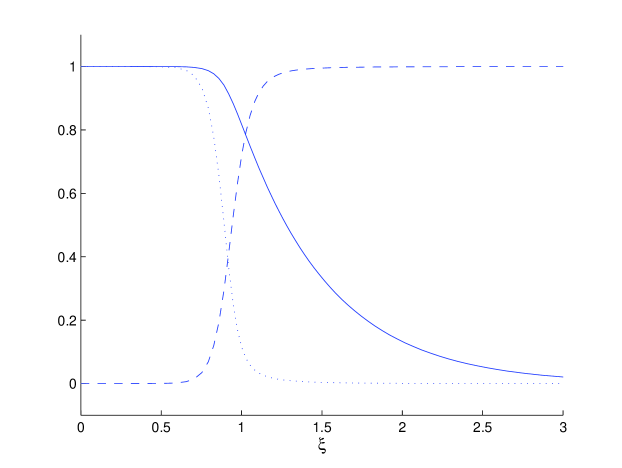
Figure 1. Front solution of the system (15) in the case $c=1.8588$, $\varepsilon=0.1$, $h=0.3$, $\sigma=0.25$, $\delta=0.0005$, and $T_{ign}=0.01$, and $Z=6$. The solid line corresponds to $u$, the dashed line to $y$, and the dotted line to $z$.

As an example of computation, Figure 1 shows the front solution as a function of $\xi$ in the case where $\varepsilon=0.1$, $h=0.3$, $\sigma=0.25$, $\delta=0.0005$, $T_{ign}=0.01$, and $Z=6$, which corresponds to the speed $c=1.8588$.

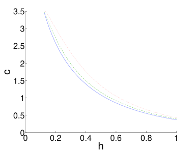
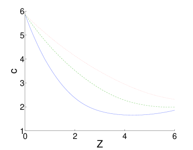
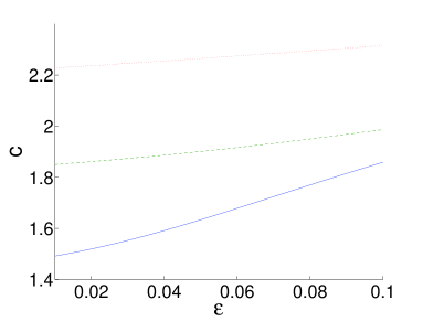
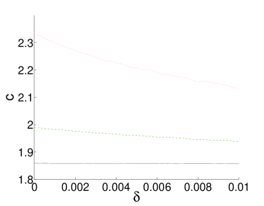
Figure 2. Plots showing the speed $c$ of the front as a function of the parameters (a) $h$ (with $\varepsilon=0.1$, $Z=6$, $\delta=0.0005$, and $T_{ign}=0.01$), (b) $Z$ (with $\varepsilon=0.1$, $h=0.3$, $\delta=0.0005$, and $T_{ign}=0.01$), (c) $\varepsilon$ (with $h=0.3$, $Z=6$, $\delta=0.0005$, and $T_{ign}=0.01$), and (d) $\delta$ (with $\varepsilon=0.1$, $h=0.3$, $Z=6$, and $T_{ign}=0.01$). In each graph, the solid line corresponds to $\sigma=0.25$, the dashed line to $\sigma=0.5$, and the dotted line to $\sigma=0.75$.

Figure 2 shows how the speed $c$ varies as a function of the various parameters. In particular, Figure 2 (d) shows $c$ as a function of $\delta$. The parameter $\delta$ is chosen so that the speed $c$ is close to the speed of the discontinuous system. For this purpose, we use $\delta=0.0005$ as we have checked that with $\delta=0.0005$, the percentage difference between the velocities of the smoothed and the discontinuous models do not exceed 2.2% in all the cases considered in this article.

4. Linearization

To analyze the stability of the front we consider the linearization of (12) about the front $(\widehat{u},\widehat{y})$. The eigenvalue problem for the linearized operator reads

(16) $$\lambda p =p_{\xi\xi}+cp_{\xi}+F_{w}({\widehat{w}})\,{\widehat{y}}\,(hp-(1-h)q)+F({\widehat{w}})q,$$

$$\lambda q =\varepsilon q_{\xi\xi}+cq_{\xi}-F_{w}({\widehat{w}})\,{\widehat{y}}\,(hp-(1-h)q)-F({\widehat{w}})q,$$

where $w=hu+(1-h)(1-y)$ and ${\widehat{w}}=w(\widehat{u},\widehat{y})$, and subscript $w$ denotes the derivative with respect to $w$. In a reaction-diffusion equation, a wave is spectrally stable in a space if the spectrum of (16) of the linearization of the system about the wave in that space is contained in the half-plane $\{\operatorname{\sf Re}\left(\lambda\right)\leq-\nu\}$ for some $\nu>0$ with the exception of a simple zero eigenvalue which is generated by the translational invariance.

4.1. Essential Spectrum

Let ${\mathcal{L}}$ be the operator defined by the right hand side of (16). To study the essential spectrum of ${\mathcal{L}}$ on the space $L^{2}$, we consider operators obtained by taking the limits of ${\mathcal{L}}$ at $\xi\to\pm\infty$, in other words, the operators obtained from ${\mathcal{L}}$ by inserting ${\widehat{y}}=1$, ${\widehat{w}}=0$, ${\widehat{y}}=0$, and ${\widehat{w}}=1$,

$${\mathcal{L}}_{\infty}=\begin{pmatrix}\frac{\mathrm{d}^{2}}{\mathrm{d}\xi^{2}}+c\frac{\mathrm{d}}{\mathrm{d}\xi}&0\\ 0&\varepsilon\frac{\mathrm{d}^{2}}{\mathrm{d}\xi^{2}}+c\frac{\mathrm{d}}{\mathrm{d}\xi}\end{pmatrix},\;\;{\mathcal{L}}_{-\infty}=\begin{pmatrix}\frac{\mathrm{d}^{2}}{\mathrm{d}\xi^{2}}+c\frac{\mathrm{d}}{\mathrm{d}\xi}&e^{(1-h)Z}\\ 0&\varepsilon\frac{\mathrm{d}^{2}}{\mathrm{d}\xi^{2}}+c\frac{\mathrm{d}}{\mathrm{d}\xi}-e^{(1-h)Z}\end{pmatrix}.$$

The spectra of the operators ${\mathcal{L}}_{\pm\infty}$ [13] is a set of curves that are included in the essential spectrum of ${\mathcal{L}}$. Moreover, the essential spectrum of ${\mathcal{L}}$ is bounded by these curves. One can find these curves from the linear dispersion relation obtained by using modes of the form $e^{\i\sigma\xi}$. This amounts to considering the quantities ${\mathcal{L}}_{\pm\infty}(\sigma)$ obtained from ${\mathcal{L}}_{\pm\infty}$ by replacing the derivative with respect to $\xi$ by $\sigma$, which in its turn implies that the spectra can be obtained by working with the equations ${\mbox{det}}\left({\mathcal{L}}_{\pm\infty}(\sigma)-\lambda I\right)=0$ (see [14] for details). It is found in [14] that since $\varepsilon<1$, the rightmost curve defined by (4.1) is $\lambda=-\varepsilon\sigma^{2}+\mathrm{i}c\sigma$, or

$$\operatorname{\sf Re}\left(\lambda\right)=-\frac{\epsilon}{c^{2}}\,\operatorname{\sf Im}\left(\lambda\right)^{2}.$$

The region to the right of this parabola and therefore the open left side of the complex plane (with the exception of the origin) can only contain point spectrum, i.e. eigenvalues with finite multiplicity.

On the other hand, the essential spectrum on the subspace of $L^{2}$ that consists of functions that decay on $+\infty$ faster than $e^{\alpha\xi}$ for some $\alpha>0$ lays strictly to the left of the imaginary axes. Indeed, substituting $(P,Q)=(p,q)e^{\alpha\xi}$ in (16) we see that the linear operators produced by the linearization about the equilibria are given by

$$\begin{split}{\mathcal{L}}_{\infty}(\alpha)&=\begin{pmatrix}\frac{\mathrm{d}^{2}}{\mathrm{d}\xi^{2}}+(c-2\alpha)\frac{\mathrm{d}}{\mathrm{d}\xi}+(\alpha^{2}-c\alpha)&0\\ 0&\varepsilon\frac{\mathrm{d}^{2}}{\mathrm{d}\xi^{2}}+(c-2\alpha)\frac{\mathrm{d}}{\mathrm{d}\xi}+(\epsilon\alpha^{2}-c\alpha)\end{pmatrix},\\ {\mathcal{L}}_{-\infty}(\alpha)&=\begin{pmatrix}\frac{\mathrm{d}^{2}}{\mathrm{d}\xi^{2}}+(c-2\alpha)\frac{\mathrm{d}}{\mathrm{d}\xi}+(\alpha^{2}-c\alpha)&e^{(1-h)Z}\\ 0&\varepsilon\frac{\mathrm{d}^{2}}{\mathrm{d}\xi^{2}}+(c-2\alpha)\frac{\mathrm{d}}{\mathrm{d}\xi}-e^{(1-h)Z}\ +(\varepsilon\alpha^{2}-c\alpha)\end{pmatrix}.\end{split}$$

Therefore on that weighted space, the right most boundary of the essential spectrum is given by $\lambda=-\varepsilon\sigma^{2}+\mathrm{i}(c-2\alpha)\sigma+(\alpha^{2}-c\alpha)$, or $\operatorname{\sf Re}\left(\lambda\right)=-\frac{\varepsilon}{(c-2\alpha)^{2}}\,\operatorname{\sf Im}\left(\lambda\right)^{2}+(\alpha^{2}-c\alpha).$ So as long as $0<\alpha<c/2$, the sign of the convection term $c-2\alpha$ is preserved and $\alpha^{2}-c\alpha<0$, the essential spectrum is to the left of the imaginary axis and its boundary has the same orientation as the boundary of the essential spectrum of the original problem.

4.2. The point spectrum.

Further in the paper, we are planning to use numerical Evans function calculation to look for unstable eigenvalues of (16). Before doing so, we first want to identify a bounded region where those eigenvalues may reside, or, in other words, to identify a subset of the right half-plane of the complex plane with a bounded complement where the unstable discrete eigenvalues are guaranteed to be absent. We accomplish this by obtaining a bound on eigenvalue $\lambda$ of the operator ${\mathcal{L}}$ under the assumption $\operatorname{\sf Re}\left(\lambda\right)\geq 0$. The following lemma holds for such $\lambda$.

Lemma 4.1.

(17) $$\begin{split}\operatorname{\sf Re}\left(\lambda\right)\int_{\mathbb{R}}|p|^{2}\,{\mbox{d}}\xi\leq h\int_{\mathbb{R}}F_{w}({\widehat{w}})\,{\widehat{y}}\,|p|^{2}\,{\mbox{d}}\xi+\int_{\mathbb{R}}(F({\widehat{w}})+(1-h)\,F_{w}({\widehat{w}})\,{\widehat{y}})\,\left(\frac{|q|^{2}}{4\epsilon_{1}}+\epsilon_{1}|p|^{2}\right)\,{\mbox{d}}\xi,\end{split}$$

and

(18) $$\begin{split}\left(\operatorname{\sf Re}\left(\lambda\right)+|\operatorname{\sf Im}\left(\lambda\right)|\right)\int_{\mathbb{R}}|p|^{2}\,{\mbox{d}}\xi&\leq\frac{c^{2}}{4}\int_{\mathbb{R}}|p|^{2}\,{\mbox{d}}\xi+h\int_{\mathbb{R}}F_{w}({\widehat{w}})\,{\widehat{y}}\,|p|^{2}\,{\mbox{d}}\xi\\ &+\int_{\mathbb{R}}\left({F({\widehat{w}})+(1-h)F_{w}({\widehat{w}})\,{\widehat{y}}}\right)\left(\frac{|q|^{2}}{2\epsilon_{1}}+\epsilon_{1}|p|^{2}\right)\,{\mbox{d}}\xi,\end{split}$$

for any real positive value of $\epsilon_{1}$.

Proof.

From the definition of $F$ it is easy to see that $F$ is a nondecreasing function of $w$ for all fixed $\sigma$ and $h$ in $[0,1]$, so its derivative is nonnegative. We multiply the first equation of (16) by $\overline{p}$ and we then integrate to obtain

(19) $$\lambda\int_{\mathbb{R}}|p|^{2}\,{\mbox{d}}\xi=c\int_{\mathbb{R}}p_{\xi}\overline{p}\,{\mbox{d}}\xi-\int_{\mathbb{R}}|p_{\xi}|^{2}\,{\mbox{d}}\xi-(1-h)\int_{\mathbb{R}}F_{w}({\widehat{w}})\,{\widehat{y}}\,q\,{\overline{p}}\,{\mbox{d}}\xi+\int_{\mathbb{R}}F({\widehat{w}})\,q\,{\overline{p}}\,{\mbox{d}}\xi+h\int_{\mathbb{R}}F_{w}({\widehat{w}})\,{\widehat{y}}\,|p|^{2}\,{\mbox{d}}\xi.$$

We take the real and imaginary parts of (19) to get

(20) $$\begin{split}\operatorname{\sf Re}\left(\lambda\right)\int_{\mathbb{R}}|p|^{2}\,{\mbox{d}}\xi=h\int_{\mathbb{R}}F_{w}({\widehat{w}})\,{\widehat{y}}\,|p|^{2}\,{\mbox{d}}\xi-\int_{\mathbb{R}}|p_{\xi}|^{2}\,{\mbox{d}}\xi+\int_{\mathbb{R}}\left(F({\widehat{w}})-(1-h){F_{w}({\widehat{w}})\,{\widehat{y}}}\right)\,\operatorname{\sf Re}\left(q\,{\overline{p}}\right)\,{\mbox{d}}\xi,\end{split}$$

and

(21) $$\begin{split}\operatorname{\sf Im}\left(\lambda\right)\int_{\mathbb{R}}|p|^{2}\,{\mbox{d}}\xi=-\mathrm{i}c\int_{\mathbb{R}}p_{\xi}\overline{p}\,{\mbox{d}}\xi+\int_{\mathbb{R}}\left(F({\widehat{w}})-(1-h){F_{w}({\widehat{w}})\,{\widehat{y}}}\right)\,\operatorname{\sf Im}\left(q\,{\overline{p}}\right)\,{\mbox{d}}\xi.\end{split}$$

Using Young’s inequality on (20), we obtain (17).

From (21), we get the following inequality

(22) $$\begin{split}|\operatorname{\sf Im}\left(\lambda\right)|\int_{\mathbb{R}}|p|^{2}\,{\mbox{d}}\xi\leq c\int_{\mathbb{R}}|p_{\xi}||{p}|\,{\mbox{d}}\xi+\int_{\mathbb{R}}\left(F({\widehat{w}})+(1-h){F_{w}({\widehat{w}})\,{\widehat{y}}}\right)\,|\operatorname{\sf Im}\left(q\,{\overline{p}}\right)|\,{\mbox{d}}\xi.\end{split}$$

Adding (20) and (22), we obtain

(23) $$\begin{split}\left(\operatorname{\sf Re}\left(\lambda\right)+|\operatorname{\sf Im}\left(\lambda\right)|\right)\int_{\mathbb{R}}|p|^{2}\,{\mbox{d}}\xi\leq c\int_{\mathbb{R}}|p_{\xi}||{p}|\,{\mbox{d}}\xi-\int_{\mathbb{R}}|p_{\xi}|^{2}\,{\mbox{d}}\xi+h\int_{\mathbb{R}}F_{w}({\widehat{w}})\,{\widehat{y}}\,|p|^{2}\,{\mbox{d}}\xi\\ +\int_{\mathbb{R}}\left(F({\widehat{w}})+(1-h){F_{w}({\widehat{w}})\,{\widehat{y}}}\right)\,\left(\operatorname{\sf Re}\left(q\,{\overline{p}}\right)+|\operatorname{\sf Im}\left(q\,{\overline{p}}\right)|\right)\,{\mbox{d}}\xi.\end{split}$$

Applying Young’s inequality ${c\,|p_{\xi}||p|\leq\frac{c^{2}|p|^{2}}{4}+|p_{\xi}|^{2}}$ to the first term of the RHS of (23) and using the fact that

$$\operatorname{\sf Re}\left(q\,{\overline{p}}\right)+|\operatorname{\sf Im}\left(q\,{\overline{p}}\right)|\leq\sqrt{2}|p||q|\leq\frac{|q|^{2}}{2\epsilon_{1}}+\epsilon_{1}|p|^{2},$$

we find (18). ∎

We next prove the following lemma.

Lemma 4.2.

(24) $$\begin{split}\operatorname{\sf Re}\left(\lambda\right)\int_{\mathbb{R}}|q|^{2}\,{\mbox{d}}\xi+\int_{\mathbb{R}}\left(F({\widehat{w}})-(1-h)F_{w}({\widehat{w}})\,{\widehat{y}}\right)|q|^{2}\,{\mbox{d}}\xi\leq h\int_{\mathbb{R}}F_{w}({\widehat{w}})\,{\widehat{y}}\,\left(\frac{|q|^{2}}{4\epsilon_{2}}+\epsilon_{2}|p|^{2}\right)\,{\mbox{d}}\xi,\end{split}$$

and

(25) $$\begin{split}\left(\operatorname{\sf Re}\left(\lambda\right)+|\operatorname{\sf Im}\left(\lambda\right)|\right)\int_{\mathbb{R}}|q|^{2}\,{\mbox{d}}\xi&\leq\frac{c^{2}}{4\varepsilon}\int_{\mathbb{R}}|q|^{2}\,{\mbox{d}}\xi+h\int_{\mathbb{R}}F_{w}({\widehat{w}})\,{\widehat{y}}\,\left(\frac{|q|^{2}}{2\epsilon_{2}}+\epsilon_{2}|p|^{2}\right)\,{\mbox{d}}\xi\\ &-\int_{\mathbb{R}}\left({F({\widehat{w}})-(1-h)F_{w}({\widehat{w}})\,{\widehat{y}}}\right)|q|^{2}\,{\mbox{d}}\xi,\end{split}$$

for any real positive value of $\epsilon_{2}$

Proof.

We multiply the second equation of (16) by $\overline{q}$, we integrate and get

(26) $$\lambda\int_{\mathbb{R}}|q|^{2}\,{\mbox{d}}\xi=c\int_{\mathbb{R}}q_{\xi}\overline{q}\,{\mbox{d}}\xi-\varepsilon\int_{\mathbb{R}}|q_{\xi}|^{2}\,{\mbox{d}}\xi-\int_{\mathbb{R}}\left(F({\widehat{w}})-(1-h)F_{w}({\widehat{w}})\,{\widehat{y}}\right)|q|^{2}\,{\mbox{d}}\xi-h\int_{\mathbb{R}}F_{w}({\widehat{w}})\,{\widehat{y}}\,p\,{\overline{q}}\,{\mbox{d}}\xi.$$

The real and imaginary parts of (26) are

(27) $$\begin{split}\operatorname{\sf Re}\left(\lambda\right)\int_{\mathbb{R}}|q|^{2}\,{\mbox{d}}\xi=-\varepsilon\int_{\mathbb{R}}|q_{\xi}|^{2}\,{\mbox{d}}\xi-\int_{\mathbb{R}}\left(F({\widehat{w}})-(1-h)F_{w}({\widehat{w}})\,{\widehat{y}}\right)|q|^{2}\,{\mbox{d}}\xi-h\int_{\mathbb{R}}F_{w}({\widehat{w}})\,{\widehat{y}}\,\operatorname{\sf Re}\left(p\,{\overline{q}}\right)\,{\mbox{d}}\xi.\end{split}$$

and

(28) $$\begin{split}\operatorname{\sf Im}\left(\lambda\right)\int_{\mathbb{R}}|q|^{2}\,{\mbox{d}}\xi=-\mathrm{i}c\int_{\mathbb{R}}q_{\xi}\overline{q}\,{\mbox{d}}\xi-h\int_{\mathbb{R}}F_{w}({\widehat{w}})\,{\widehat{y}}\,\operatorname{\sf Im}\left(p\,{\overline{q}}\right)\,{\mbox{d}}\xi.\end{split}$$

Using Young’s inequality on (27), we get (24).

From (28), we get the inequality

(29) $$\begin{split}|\operatorname{\sf Im}\left(\lambda\right)|\int_{\mathbb{R}}|q|^{2}\,{\mbox{d}}\xi\leq c\int_{\mathbb{R}}|q_{\xi}||{q}|\,{\mbox{d}}\xi+h\int_{\mathbb{R}}F_{w}({\widehat{w}})\,{\widehat{y}}\,\left|\operatorname{\sf Im}\left(p\,{\overline{q}}\right)\right|\,{\mbox{d}}\xi.\end{split}$$

Adding (27) and (29), we obtain

(30) $$\begin{split}\left(\operatorname{\sf Re}\left(\lambda\right)+|\operatorname{\sf Im}\left(\lambda\right)|\right)\int_{\mathbb{R}}|q|^{2}\,{\mbox{d}}\xi\leq c\int_{\mathbb{R}}|q_{\xi}||{q}|\,{\mbox{d}}\xi+h\int_{\mathbb{R}}F_{w}({\widehat{w}})\,{\widehat{y}}\,\left(\left|\operatorname{\sf Im}\left(p\,{\overline{q}}\right)\right|-\operatorname{\sf Re}\left(p\,{\overline{q}}\right)\right)\,{\mbox{d}}\xi\\ -\varepsilon\int_{\mathbb{R}}|q_{\xi}|^{2}\,{\mbox{d}}\xi-\int_{\mathbb{R}}\left(F({\widehat{w}})-(1-h)F_{w}({\widehat{w}})\,{\widehat{y}}\right)|q|^{2}\,{\mbox{d}}\xi.\end{split}$$

Applying Young’s inequality to $c|q||q_{\xi}|$ in the first term of the RHS of (30) in the form

$$c|q||q_{\xi}|\leq\frac{c^{2}|q|^{2}}{4\varepsilon}+\varepsilon|q_{\xi}|^{2},$$

and the fact that

$$\left|\operatorname{\sf Im}\left(q\,{\overline{p}}\right)\right|-\operatorname{\sf Re}\left(q\,{\overline{p}}\right)\leq\sqrt{2}|p||q|\leq\frac{|q|^{2}}{2\epsilon_{2}}+\epsilon_{2}|p|^{2},$$

we find (25). ∎

The following theorem holds.

Theorem 4.3.

If $\lambda\neq 0$ is an eigenvalue for (16) with nonnegative real part, then we have the following inequalities:

(31) $$\begin{split}\operatorname{\sf Re}\left(\lambda\right)\leq\left(3-\frac{3h}{2}\right)\sup_{\mathbb{R}}(F_{{w}}({\widehat{w}})\,{\widehat{y}})+\mathrm{exp}\left(Z(1-h)\right),\end{split}$$

and

(32) $$\begin{split}|\lambda|\leq\frac{c^{2}}{4}\max{\left\{1,\,\frac{1}{\varepsilon}\right\}}+\left(3-h\right)\sup_{\mathbb{R}}(F_{{w}}({\widehat{w}})\,{\widehat{y}})+\mathrm{exp}\left(Z(1-h)\right).\end{split}$$

Proof.

Multiplying (17) by $\theta$ and adding (24), we obtain

$$\begin{split}\operatorname{\sf Re}\left(\lambda\right)\int_{\mathbb{R}}(\theta|p|^{2}+|q|^{2})\,{\mbox{d}}\xi\leq\left((\theta+\epsilon_{2})\,h+\epsilon_{1}\theta(1-h)\right)\int_{\mathbb{R}}F_{w}({\widehat{w}})\,{\widehat{y}}\,|p|^{2}\,{\mbox{d}}\xi\\ +\left(1-h+\frac{h}{4\epsilon_{2}}+\frac{\theta(1-h)}{4\epsilon_{1}}\right)\int_{\mathbb{R}}F_{w}({\widehat{w}})\,{\widehat{y}}\,|q|^{2}\,{\mbox{d}}\xi+\\ \left(\frac{\theta}{4\epsilon_{1}}-1\right)\int_{\mathbb{R}}F({\widehat{w}})\,|q|^{2}\,{\mbox{d}}\xi+\epsilon_{1}\theta\int_{\mathbb{R}}F({\widehat{w}})|p|^{2}\,{\mbox{d}}\xi.\end{split}$$

Next we choose $\theta=4$ and $\epsilon_{1}=\epsilon_{2}=1$ and obtain

(33) $$\begin{split}\operatorname{\sf Re}\left(\lambda\right)\int_{\mathbb{R}}(4|p|^{2}+|q|^{2})\,{\mbox{d}}\xi\leq\left(\frac{h}{4}+1\right)\int_{\mathbb{R}}F_{w}({\widehat{w}})\,{\widehat{y}}\,4|p|^{2}\,{\mbox{d}}\xi\\ +\left(2-\frac{7h}{4}\right)\int_{\mathbb{R}}F_{w}({\widehat{w}})\,{\widehat{y}}\,|q|^{2}\,{\mbox{d}}\xi+\int_{\mathbb{R}}F({\widehat{w}})\,4|p|^{2}\,{\mbox{d}}\xi.\end{split}$$

Since $F$ is nondecreasing,

(34) $$\begin{split}\displaystyle{\sup_{x\in\mathbb{R}}\left(F({\widehat{w}})\right)=F(1)=\mathrm{exp}\left(Z(1-h)\right)}.\end{split}$$

The inequality (31) then follows from using (34) in (33).

We then multiply (18) by $\theta$ and add (25) to obtain

$$\begin{split}&\left(\operatorname{\sf Re}\left(\lambda\right)+|\operatorname{\sf Im}\left(\lambda\right)|\right)\int_{\mathbb{R}}\left(\theta|p|^{2}+|q|^{2}\right)\,{\mbox{d}}\xi\\ &\leq\frac{c^{2}}{4}\max{\left\{1,\,\frac{1}{\varepsilon}\right\}}\int_{\mathbb{R}}\left(\theta|p|^{2}+|q|^{2}\right)\,{\mbox{d}}\xi+\left(\frac{\theta}{2\epsilon_{1}}-1\right)\int_{\mathbb{R}}{F({\widehat{w}})}|q|^{2}\,{\mbox{d}}\xi\\ &+\epsilon_{1}\int_{\mathbb{R}}{F({\widehat{w}})}\,\theta\,|p|^{2}\,{\mbox{d}}\xi+\left(\frac{h\epsilon_{2}}{\theta}+h+(1-h)\epsilon_{1}\right)\int_{\mathbb{R}}F_{w}({\widehat{w}})\,{\widehat{y}}\,\theta\,|p|^{2}\,{\mbox{d}}\xi\\ &+\left(\frac{\theta(1-h)}{2\epsilon_{1}}+\frac{h}{2\epsilon_{2}}+1-h\right)\int_{\mathbb{R}}F_{w}({\widehat{w}})\,{\widehat{y}}\,|q|^{2}\,{\mbox{d}}\xi.\end{split}$$

Here, we choose $\theta=2$ and $\epsilon_{1}=\epsilon_{2}=1$ and get

$$\begin{split}&\left(\operatorname{\sf Re}\left(\lambda\right)+|\operatorname{\sf Im}\left(\lambda\right)|\right)\int_{\mathbb{R}}\left(2|p|^{2}+|q|^{2}\right)\,{\mbox{d}}\xi\leq\frac{c^{2}}{4}\max{\left\{1,\,\frac{1}{\varepsilon}\right\}}\int_{\mathbb{R}}\left(2|p|^{2}+|q|^{2}\right)\,{\mbox{d}}\xi\\ &+\int_{\mathbb{R}}{F({\widehat{w}})}\,2\,|p|^{2}\,{\mbox{d}}\xi+\left(\frac{h}{2}+1\right)\int_{\mathbb{R}}F_{w}({\widehat{w}})\,{\widehat{y}}\,2\,|p|^{2}\,{\mbox{d}}\xi+\left(2-\frac{3h}{2}\right)\int_{\mathbb{R}}F_{w}({\widehat{w}})\,{\widehat{y}}\,|q|^{2}\,{\mbox{d}}\xi.\end{split}$$

Finally, using (34), we obtain

$$\begin{split}\left(\operatorname{\sf Re}\left(\lambda\right)+|\operatorname{\sf Im}\left(\lambda\right)|\right)\leq\frac{c^{2}}{4}\max{\left\{1,\,\frac{1}{\varepsilon}\right\}}+\left(3-h\right)M+\mathrm{exp}\left(Z(1-h)\right).\end{split}$$

The fact that $|\lambda|\leq\operatorname{\sf Re}\left(\lambda\right)+|\operatorname{\sf Im}\left(\lambda\right)|$ when $\operatorname{\sf Re}\left(\lambda\right)\geq 0$ then implies (32). ∎

5. Linear Stability

The system (16) can be turned into a linear dynamical system of the form

(35) $$X^{\prime}=A(\xi,\lambda)\,X,$$

where $A$ is the $4\times 4$ following square matrix

(36) $$\begin{split}A(\xi,\lambda)=\left(\begin{array}[]{cccc}0&1&0&0\\ \lambda-h\,F_{w}({\widehat{w}})\,{\widehat{y}}&-c&(1-h)\,F_{w}({\widehat{w}})\,{\widehat{y}}-F({\widehat{w}})&0\\ 0&0&0&1\\ h\,F_{w}({\widehat{w}})\,{\widehat{y}}/\varepsilon&0&\left(\lambda+(1-h)\,F_{w}({\widehat{w}}){\widehat{y}}+F({\widehat{w}})\right)/\varepsilon&-c/\varepsilon\end{array}\right).\end{split}$$

The asymptotic behavior as $\xi\rightarrow\infty$ of the solutions to (35) is determined by the matrices

$${\mathcal{A}}^{\infty}(\lambda)=\lim_{\xi\rightarrow\infty}A(\xi,\lambda),$$

which is found by inserting the values ${\widehat{y}}=1$ and ${\widehat{w}}=0$ into (36)

(37) $$\begin{split}{\mathcal{A}}^{\infty}(\lambda)=\begin{pmatrix}0&1&0&0\\ \lambda&-c&0&0\\ 0&0&0&1\\ 0&0&\lambda/\varepsilon&-c/\varepsilon\end{pmatrix}.\end{split}$$

For $\operatorname{\sf Re}\left(\lambda\right)>0$, the matrix of ${\mathcal{A}}^{\infty}$ has two eigenvalues with negative real part. They are given by

(38) $$\mu_{1+}=-\frac{1}{2\varepsilon}(c+\sqrt{c^{2}+4\varepsilon\lambda}),\,\,\,\mu_{2+}=-\frac{1}{2}(c+\sqrt{c^{2}+4\lambda}),$$

and their corresponding eigenvectors are

$$v_{1+}=\left(0,0,1,\mu_{1+}\right)^{T},\;\;\;\;v_{2+}=\left(1,\mu_{2+},0,0\right)^{T}.$$

The asymptotic behavior as $\xi\rightarrow-\infty$ of the solutions to (35) is determined by the matrix

$$\begin{split}{\mathcal{A}}^{-\infty}(\lambda)=\lim_{\xi\rightarrow-\infty}A(\xi,\lambda),\end{split}$$

which is found by inserting the values ${\widehat{y}}=0$ and ${\widehat{w}}=1$ into (36)

(39) $$\begin{split}{\mathcal{A}}^{-\infty}(\lambda)=\begin{pmatrix}0&1&0&0\\ \lambda&-c&e^{(1-h)Z}&0\\ 0&0&0&1\\ 0&0&(\lambda+e^{(1-h)Z})/\varepsilon&-c/\varepsilon\end{pmatrix}.\end{split}$$

For $\operatorname{\sf Re}\left(\lambda\right)>0$, the matrix ${\mathcal{A}}^{-\infty}$ has two eigenvalues with positive real part. They are given by

(40) $$\begin{split}\mu_{1-}=-\frac{1}{2\varepsilon}\left(c-\sqrt{c^{2}+4\varepsilon\lambda+4\varepsilon e^{Z(1-h)}}\right),\quad\mu_{2-}=-\frac{1}{2}\left(c-\sqrt{c^{2}+4\lambda}\right),\end{split}$$

and their corresponding eigenvectors are

$$\begin{split}v_{1-}=&\left(1,\mu_{1-},\frac{(1-\varepsilon)(\lambda-c\,\mu_{1-})}{\varepsilon\,e^{Z(1-h)}}+\frac{1}{\varepsilon},{\frac{\left(\left({c}^{2}+\lambda\,\varepsilon\right)\left(1-\varepsilon\right)+\varepsilon\,e^{Z(1-h)}\right){\it\mu_{1-}}-c\left(\lambda+e^{Z(1-h)}\right)\left(1-\varepsilon\right)}{{\varepsilon}^{2}e^{Z(1-h)}}}\right)^{T},\\ v_{2-}=&\left(1,\,\mu_{2-},0,0\right)^{T}.\end{split}$$

As a consequence [16], the system (35) has two linearly independent solutions $X_{1+}$ and $X_{2+}$ converging to zero as $\xi\rightarrow\infty$ and two solutions $X_{1-}$ and $X_{2-}$ converging to zero as $\xi\rightarrow-\infty$, satisfying

$$\lim_{\xi\rightarrow\pm\infty}X_{i\pm}e^{-\mu_{i\pm}\xi}=v_{i\pm},\;\;i=1,2.$$

Clearly, a value of $\lambda$ is an eigenvalue for the problem (16) if and only if the space of solutions of (35) bounded as $\xi\rightarrow+\infty$, spanned by $\{X_{1+},\,X_{2+}\}$, and the space of solutions bounded as $\xi\rightarrow-\infty$, spanned by $\{X_{1-},\,X_{2-}\}$, have an intersection of strictly positive dimension. Those values of $\lambda$ can be located with the help of the Evans function [18, 20, 26, 17, 24, 19, 22, 25, 21, 23]. The Evans function is a function of the spectral parameter $\lambda$; it is analytic, real for $\lambda$ real, and it vanishes on the point spectrum of the problem (16). There are several definitions of the Evans function. For our purpose of numerical computations, we use the definition involving exterior algebra [27, 28, 29, 30, 31, 32, 34, 35, 33].

We are in the situation where the dimension of the system is $n=4$ and the dimensions of the stable and unstable manifolds are $n_{s}=n_{u}=2$. In such a case, we consider the wedge-space $\bigwedge^{2}({\mathbb{C}}^{4})$, the space of all two forms on ${\mathbb{C}}^{4}$. The induced dynamics of (35) on $\bigwedge^{2}({\mathbb{C}}^{4})$ can be written as

(41) $${U}^{\prime}={\bf A}^{(2)}(\xi,\lambda){U}.$$

Here the matrix ${A}^{(2)}$ is matrix generated by ${A}=\{a_{ij}\}$ on the wedge-space $\bigwedge^{2}({\mathbb{C}}^{4})$. Using the standard basis of $\bigwedge^{2}({\mathbb{C}}^{4})$,

(42) $$\begin{array}[]{l}{\bf\omega}_{1}={\bf e}_{1}\wedge{\bf e}_{2},\quad{\bf\omega}_{2}={\bf e}_{1}\wedge{\bf e}_{3},\quad{\bf\omega}_{3}={\bf e}_{1}\wedge{\bf e}_{4},\\ {\bf\omega}_{4}={\bf e}_{2}\wedge{\bf e}_{3},\quad{\bf\omega}_{5}={\bf e}_{2}\wedge{\bf e}_{4},\quad{\bf\omega}_{6}={\bf e}_{3}\wedge{\bf e}_{4},\end{array}$$

where $\left\{{\bf e}_{1},{\bf e}_{2},{\bf e}_{3},{\bf e}_{4}\right\}$ is the standard basis of ${\mathbb{C}}^{4}$, the matrix ${A}^{(2)}$ is given by

$${A}^{(2)}=\left(\begin{array}[]{ccccccccccc}a_{11}\!+\!a_{22}&&a_{23}&&a_{24}&&-a_{13}&&-a_{14}&&0\\ a_{32}&&a_{11}\!+\!a_{33}&&a_{34}&&a_{12}&&0&&-a_{14}\\ a_{42}&&a_{43}&&a_{11}\!+\!a_{44}&&0&&a_{12}&&a_{13}\\ -a_{31}&&a_{21}&&0&&a_{22}\!+\!a_{33}&&a_{34}&&-a_{24}\\ -a_{41}&&0&&a_{21}&&a_{43}&&a_{22}\!+\!a_{44}&&a_{23}\\ 0&&-a_{41}&&a_{31}&&-a_{42}&&a_{32}&&a_{33}\!+\!a_{44}\end{array}\right).$$

In our case, the asymptotic matrices are given by

$$\lim_{\xi\to\pm\infty}{A}^{(2)}(\xi,\lambda)=\left({\mathcal{A}}^{\pm\infty}\right)^{(2)},$$

where ${\mathcal{A}}^{\pm\infty}$ are as in (37) and (39). The eigenvalue of $\left({\mathcal{A}}^{\infty}\right)^{(2)}$ with the smallest real part is $\mu_{1+}+\mu_{2+}$ with eigenvector $v_{1+}\wedge v_{2+}$. The solution of (41) given by $U_{+}=X_{1+}\wedge X_{2+}$ then behaves as

$$\lim_{\xi\rightarrow\infty}U_{+}e^{-(\mu_{1+}+\mu_{1+})\xi}=w_{+}\equiv v_{1+}\wedge v_{2+}.$$

Similarly, the solution $U_{-}=X_{1-}\wedge X_{2-}$ behaves as

$$\lim_{\xi\rightarrow-\infty}U_{-}e^{-(\mu_{1-}+\mu_{-})\xi}=w_{-}\equiv v_{1-}\wedge v_{2-}.$$

This allows us to define the Evans function as

$$E(\lambda)\equiv{U}_{-}\wedge{U}_{+},$$

where $U_{\pm}$ are evaluated at some chosen value of $\xi$ (often taken to be $\xi=0$). If $U$ is written in components in the basis (42), then the Evans function is computed [28, 36, 30] as

$$E(\lambda)={{U}_{-}^{T}}\,\Sigma\,{U}_{+},$$

where ${\Sigma}$ is the matrix

$${\bf\Sigma}=\left[\begin{array}[]{ccccccccc}0&\hfill 0&\hfill 0&\hfill 0&\hfill 0&1\\ 0&\hfill 0&\hfill 0&\hfill 0&-1&0\\ 0&\hfill 0&\hfill 0&\hphantom{-}1&\hfill 0&0\\ 0&\hfill 0&\hphantom{-}1&\hfill 0&\hfill 0&0\\ 0&-1&\hfill 0&\hfill 0&\hfill 0&0\\ 1&\hfill 0&\hfill 0&\hfill 0&\hfill 0&0\end{array}\right].$$

The function $E(\lambda)$ will be analytic in the any region of the complex plane where the eigenvalues $\mu_{1+}+\mu_{2+}$ and $\mu_{1-}+\mu_{2-}$ are, respectively, the eigenvalues with smallest and largest real part of $\left({\mathcal{A}}^{\infty}\right)^{(2)}$ and $\left({\mathcal{A}}^{-\infty}\right)^{(2)}$. In view of the expressions for the eigenvalues given in (38) and (40), to define such a region, it suffices to implement the condition

(43) $$\operatorname{\sf Re}\left(\lambda\right)>-\frac{1}{4}\min{\left(1,\,\frac{1}{\varepsilon}\right)}.$$

To compute the Evans numerically, we choose a positive value $\xi=L$ at which the matrix given $A$ is suitably close to its asymptotic value ${\mathcal{A}}^{\infty}$. We then use ODE45 to integrate the system (41) backward from $\xi=L$ in the direction of the eigenvector $w_{+}$ and find $U_{+}$ (with the ODE45 absolute and relative error tolerances both set to $10^{-10}$). Additionally, in order to eliminate the exponential growth due to the eigenvalue with negative real part as we integrate from $\xi=L$, we modify the system (41) in the following way

(44) $$U^{\prime}=\left(A^{(2)}-(\mu_{1+}+\mu_{2+})I\right)\,U,$$

and use the initial condition $U(L)=w_{+}$. To find $U_{-}$, we integrate the following modified version of (41)

(45) $$U^{\prime}=\left(A^{(2)}-(\mu_{1-}+\mu_{2-})I\right)\,U,$$

frontward from $\xi=0$ with initial condition $U(0)=w_{-}$, (recall that $\xi=0$ is the value of $\xi$ from which the front was computed (see Section 3)). The Evans function then is taken to be the quantity ${{U}_{-}^{T}}\,\Sigma\,{U}_{+}$ evaluated at the value $\xi=\xi^{*}$ at which the front solution of (15) satisfies $u(\xi^{*})=y(\xi^{*})$ (in Figure 1, this corresponds to the value of $\xi$ at which the solid and dashed lines meet). Note that in the numerical computations, we choose the eigenvectors $w_{\pm}$ so that ${{w}_{-}^{T}}\,\Sigma\,{w}_{+}=1$. Note also that in our case, since $F(w)=0$ for $w<v_{ign}$, the matrix $A$ in (36) reaches the constant matrix $A^{\infty}$ for a finite positive value of $\xi$. When computing $X_{+}$, we thus choose the value of $L$ to be greater than the lowest value of $\xi$ satisfying ${\widehat{w}}(\xi)<T_{ign}$.

Since we are interested in the zeroes of the Evans function, the standard method is to compute the integral of the logarithmic derivative of the Evans function on a given closed curve and obtain the winding number of $E(\lambda)$ along that curve. In our case, the contour of integration is chosen so that it lies in the region defined by (43) and so that its interior encloses the intersection of the right side of the complex plane and the region defined by (32). For example, in the case $\varepsilon=0.1$, $h=0.3$, $Z=6$, $\sigma=0.25$, $\delta=0.0005$, and $T_{ign}=0.01$ we find the RHS of (32) to be $187.4478$ and $c$ to be $1.8588$. For the computation of the Evans function, we find that we can take $L$ to be 2.7786 and our numerical winding number computation then shows that the Evans function has no zeroes other than the one at the origin. Note that the eigenvalue at $\lambda=0$ is due to the translation invariance of the system (9). We have made the same computations for several values of $h$ and $\sigma$ between 0 and 1 (specifically for $h=0.3,0.6,0.9$ and $\sigma=0.25,0.5,0.75$), and for $Z=4,5,6$ (with $\varepsilon=0.1$, $\delta=0.0005$, and $T_{ign}=0.01$). Every time, we have found the eigenvalue at the origin to be the only one. This thus strongly suggests that there is a regime in which the front solution is spectrally stable, with the exception of essential spectrum touching the imaginary axis.

Note that there is a special parameter regime where $F$ in System (9) is a function of one variable only and where System (9) is related to a well-studied combustion model. As we explain below, this connection indicates that there are parameter regimes when the wave in (9) is unstable. Indeed, when $h=1$, $\sigma=0$, $\delta=T_{ign}=0$, the function $F$ in (5) reduces to $F=e^{-1/u}$ and System (9) can be scaled to the well studied case of the model (11). More precisely, if one uses the change of variables $\widetilde{u}=u/Z$, $\widetilde{y}=y$, $t=(Z/e^{Z})\widetilde{t}$, and $x=\sqrt{Z/e^{Z}}\,\widetilde{x}$, then system (9), becomes

(46) $$\begin{split}u_{t}&=u_{xx}+yF(u),\\ y_{t}&={{\color[rgb]{0,0,0}\varepsilon}}y_{xx}-ZyF(u).\end{split}$$

System (46) is a combustion model with large Lewis number ${\rm{Le}}=1/\varepsilon$ [38, 39, 33, 37] for which there is an instability occurring at about $Z=6.5$ for small $\varepsilon$ [40, 15, 33]. This instability is caused by a pair of conjugate eigenvalues crossing the imaginary axis to the right side of the complex plane [15, 33]. To obtain an example of instability in our model, we use the fact that we know an instability for System (46) above and the fact that System (9) is equivalent to System (46) for a specific set of parameter values. We consider sets of parameters close the values $h=1$, $\sigma=0$, $\delta=T_{ign}=0$ for which (9) is equivalent to System (46). Specifically, we consider the set of parameter values: $\varepsilon=0.01$, $h=1$, $\sigma=0$, $\delta=0.0005$, and $T_{ign}=0.01$ in System (9). In this case, we find a pair of eigenvalues $\lambda=\pm 0.1692\mathrm{i}$ when $Z=6.578$. These two eigenvalues move to the right side of the complex plane when $Z$ is increased. If we increase the value of $\varepsilon$ to 0.1, and keep the other parameters the same, the pair of eigenvalues occur for $Z=7.036$ at $\lambda=\pm 0.1088\mathrm{i}$. Note that in order to locate an eigenvalue, we use the fact that (as mentioned before) the integral of the logarithmic derivative of an analytic function $f$ along a closed curve $\Gamma$ can be used to obtained the number of zeroes inside that curve together with the fact that the integral

$$\frac{1}{2\pi\mathrm{i}}\oint_{\Gamma}\frac{zf^{\prime}}{f}dz$$

gives the sum of the zeroes inside $\Gamma$. We numerically compute these integrals to locate zeroes of the Evans function in a given domain. Generally, this technique is known as the method of moments [15, 41, 42]. However, since in our case we are only looking for one root at a time only, the use of the higher moments (where $z$ is replaced by $z^{n}$) is not necessary.

6. Convective instability.

As we showed above there are parameter regimes when the linearization of the system (12) around the front has no unstable discrete spectrum, but has essential spectrum that extends to imaginary axes. We have checked in Section  4.1 that this spectrum can be moved to the left of the imaginary axis by a weight $\rm e^{\alpha\xi}$, $\alpha>0$, therefore, on the linear level, the instability of the front is convective, i.e. perturbations to the front that are localized sufficiently close to its tail do not influence the dynamics near the interface of the front. In the frame moving with the front the perturbations are transported towards $-\infty$ and are guaranteed to grow no faster than the reciprocal of the exponential weight. In this section we study whether this is the case on the nonlinear level as well. More precisely, we show that Theorems 3.14 and 3.16 from [43] apply and describe their conclusions.

First, we check that the nonlinearity in (12) satisfies the conditions of the mentioned above theorems. Recall that the front $(\widehat{u}(\xi),\widehat{y}(\xi))$ satisfies boundary conditions $(u,y)\to(1,0)$ as $\xi\to-\infty$, and $(u,y)\to(0,1)$ as $\xi\to+\infty$. Theorems 3.14 and 3.16 from [43] are formulated for a system that supports a front that approaches the zero state at $-\infty$. Therefore we rewrite (12) in terms of a new variable $r=u-1$,

(47) $$r_{t}= r_{\xi\xi}+cr_{\xi}+yF(h(r+1)+(1-h)(1-y)),$$

$$y_{t}= \varepsilon y_{\xi\xi}+cy_{\xi}-yF(h(r+1)+(1-h)(1-y)).$$

This system has equilibria $(0,0)$ and $(-1,1)$. We write the reaction term of (47) in vector notation that are used in [43]

$$R(r,y)=\begin{pmatrix}yF(h(r+1)+(1-h)(1-y))\\ -yF(h(r+1)+(1-h)(1-y))\end{pmatrix}.$$

For the results of [43] to hold, function $R$ should be in $R\in C^{3}$, therefore here we do not consider the reaction term with a jump, but only the smooth version of it given by (5). It is easy to see that $R(r,0)\equiv 0$ for any $r$, so the linearization of the system (47) about the equilibrium $(0,0)$ has a triangular structure that implies that the evolution of the perturbation $\tilde{y}$ to the $y=0$ component is independent of the behavior of the perturbation $\tilde{r}$ to the $r=0$ component,

(48) $$\tilde{r}_{t}= \tilde{r}_{\xi\xi}+c\tilde{r}_{\xi}+F(1)\tilde{y},$$

$$\tilde{y}_{t}= \varepsilon\tilde{y}_{\xi\xi}+c\tilde{y}_{\xi}-F(1)\tilde{y}.$$

Let us turn our attention to the operator that is given by the right hand side of (48),

$$L\begin{pmatrix}\tilde{r}\\ \tilde{y}\end{pmatrix}=\begin{pmatrix}\partial_{\xi\xi}+c\partial_{\xi}&F(1)\\ 0&\varepsilon\partial_{\xi\xi}+c\partial_{\xi}-F(1)\end{pmatrix}\begin{pmatrix}\tilde{r}\\ \tilde{y}\end{pmatrix}.$$

For the theorems that we wish to apply, it is important that the linear operator $\varepsilon\partial_{\xi\xi}+c\partial_{\xi}-F(1)$ has strictly negative spectrum, and therefore the perturbation $\tilde{y}$ decays in time exponentially, and the operator $\partial_{\xi\xi}+c\partial_{\xi}$ generates a bounded semigroup on the space $L^{2}$.

The second set of conditions is concerned with the properties of the front and the linearization of (47) about it. We know from the geometric construction [8] that the front we consider converges to its rest states at exponential rates. We also know from Section 4.1 that the marginally stable essential spectrum is moved to the left of the imaginary axis by the weight $e^{\alpha\xi}$ for $0<\alpha<c/2$. We then choose $\alpha$ so small that each of the components of the derivative of the front $(\widehat{u\,}^{\prime}(\xi),\widehat{y\,}^{\prime}(\xi))$ belongs to the weighted Sobolev space $L_{\alpha}^{2}$ which for us is a space of functions $f$ such that $f(\xi)e^{\alpha\xi}\in L^{2}$.

Thus all of the hypothesis of theorems 3.14 and 3.16 from [43] hold.

Theorems 3.14 and Theorem 3.16 then imply a result which is similar to Theorems 6.1 and 6.2 in [9] which were obtained for a reduction of the original system corresponding to $\epsilon=0$ case. We refer the reader to [9] for the exact formulations and physical interpretations and here just give a description of the obtained for the System (12) results. Suppose that initially the perturbations to the front are small in both regular norm (either $H^{1}$ or $BUC$) and the weighted norm, then in the weighted norm the perturbations to all components of the front decay exponentially fast, in other words, the front is orbitally stable with asymptotic phase; in the regular norm, the perturbation to $y$ component decays exponentially in the norm without the weight, but the perturbation to the $u$ component stays only bounded. Theorem 3.16 in [43] implies that if the initial perturbation in addition are small in $L^{1}$-norm, then the perturbation to the $u$-component decays diffusively in $L_{\infty}$-norm. The similarity of the nonlinear stability results should not be surprising cresince the fronts considered here and in [9] correspond to different, singular reductions of the same system.

7. Discussion and conclusion

In this paper, we have considered Model (1) describing combustion in inert porous media under condition of high hydraulic resistance. This model can be scaled to System (2) and we were interested in traveling front solutions, whose existence and unicity was established in [6, 7]. Assuming that the Lewis number has the special value ${{{\rm{Le}}^{-1}=\gamma(1-\mu)}}$, the system can be written as (2). Furthermore, assuming that the initial conditions (8) hold, the system can be reduced to (9) (first obtained in [2, 4]). While our study focussed on this reduced system, we show below that the results obtained in this article still hold if (8) is not satisfied. Concerning the reduced system (9), we were interested in the stability analysis of the traveling front solutions which satisfy the boundary conditions (14). We have considered the eigenvalue problem arising from the linearization of the equations about the front solutions. However, in order to have a well-defined linear operator, we have opted for a smooth version of the reaction term (5) that can be made as close as desired to the discontinuous version given in (1). In a weighted version of $L^{2}$, the essential spectrum was shown to lie in the open left side of the complex plane. As far as the point spectrum goes, we have performed an energy estimate computation to obtain an upper bound on the modulus of any possible eigenvalue with non-negative real part. Using this bound, we have used a numerical winding number computation of the Evans function to show that there are parameter regimes for which there are no eigenvalues on the right side of the complex plane. Specifically, we have considered an array of values of $h$ and $\sigma$ between 0 and 1 ($h=0.3,0.6,0.9$ and $\sigma=0.25,0.5,0.75$) for $Z=4,5,6$, while keeping $\varepsilon=0.1$, $\delta=0.0005$, and $T_{ign}=0.01$. For the parameter regimes with no unstable discrete spectrum, we further have proved that the instability caused by the essential spectrum is convective, which means perturbations to the front that are localized sufficiently close to its tail do not influence the dynamics near the interface of the front.

We would now like to show how our results extend to the case where the initial condition (8) do not hold. Concerning the spectral stability, if we remove the initial condition given in (8) but still consider the value ${{{\rm{Le}}^{-1}=\gamma(1-\mu)}}$, then the system (2) becomes (2) and thus differs from the reduced system (9) by the addition of the heat equation $g_{t}=\varepsilon g_{xx}$. The eigenvalue problem corresponding to the heat equation has no point spectrum and its continuous spectrum is restricted to the open left side of the complex plane except for the point at the origin. As a consequence, the results obtained about the spectral stability obtained for the reduced system (9) still hold for the system (2) which is full system (2) (or (1)) in the special case where ${{{\rm{Le}}^{-1}=\gamma(1-\mu)}}$. For the nonlinear stability, we perform an analysis similar to that in Section 6. It is easy to see that theorems 3.14 and 3.16 from [43] are applicable to System (2) as well. We conclude that the time evolution of perturbations to the $u$ and $y$ components are the same as in reduced system (9). In case when initial perturbations to the front are small in both regular $H^{1}$ or $BUC$ norm and in the weighted norm, the additional, $g$ component stays bounded in the norm without the weight and decays exponentially in the weighted norm. Taking into account behavior of the perturbations to the $y$ component which decays exponentially in all norms, we can conclude that perturbations to the original $v$-component behave the same way as perturbations to $g$. If, in addition, initial perturbations are also small in $L^{1}$-norm, then the perturbations to $g$, and therefore $v$-components of the front not only stay bounded but also decay algebraically in $L_{\infty}$-norm.

We point out that the stability of the fronts in the full Model (1) for values of the Lewis number other than the one considered here is still an open question and will be a subject of our future research. As mentioned above, the cases of $\epsilon=0$ considered in our previous paper [9] is singular and the results obtained for that case do not imply that similar results have to hold for the Model (1) in general.

To conclude, in this paper we investigated the stability of fronts for a specific value of the Lewis number. To do so, we have first considered one of the known singular reductions of Model (1). The singular reduction considered here is based on choosing a special value of the Lewis number which is a parameter that is not present in the other singular perturbation of (1) studied in [9] (when $\epsilon=0$). Although the analysis follows the same sequence of steps as in [9] for stability analysis of fronts such as spectral stability and the proof of the nonlinear stability for marginally stable spectrum, from the technical point of view it is significantly different from the one performed in [9]. This can be easily understood by the fact that setting $\epsilon=0$ in (1) changes the nature of the system of PDEs since it reduces the order by 2. The results of this article show that the fronts that the full model (1) exhibits for ${{{\rm{Le}}^{-1}=\gamma(1-\mu)}}$ are indeed physical because they are in some sense stable.

Funding statement. This work was supported by the National Science Foundation through grants DMS-1311313 (A. Ghazaryan) and DMS-0908074 (S. Lafortune).

References

- [1] Brailovsky I, Goldshtein V, Shreiber I, Sivashinsky G. 1997 On combustion waves driven by diffusion of pressure, Combust. Sci. Tech., 124, 145-165.
- [2] Gordon P, Ryzhik L. 2006 Traveling fronts in porous media: existence and a singular limit, Proc. Roy. Soc. London Ser. A, 462, 1965-1985.
- [3] Brailovsky I, Kagan L, Sivashinsky GI. 2012 Combustion waves in hydraulically resisted systems, Phil. Trans. R. Soc. A 370, 625-646.
- [4] Gordon PV. 2007 Recent mathematical results on combustion in hydraulically resistant porous media, Math. Model. Nat. Phenom. 2 56-76.
- [5] Sivashinsky GI. 2002 Some developments in premixed combustion modeling, Proceedings of the Combustion Institute, 29, 1737-1761.
- [6] Dkhil F. 2004 Travelling wave solutions in a model for filtration combustion, Nonlinear Analysis 58, 395-415.
- [7] Gordon PV, Kamin S, Sivashinsky GI. 2002 On initiation of subsonic detonation in porous media combustion, Asymptot. Anal., 29, 309-321.
- [8] Ghazaryan A, Gordon P, Jones C. 2007 Traveling waves in porous media combustion: Uniqueness of waves for small thermal diffusivity, J. of Dynamics and Differential Equations 19, 951-966.
- [9] Ghazaryan A, Lafortune S, McLarnan P. 2015 Stability analysis for combustion fronts traveling in hydraulically resistant porous media, SIAM J. on Applied Mathematics
- [10] Khudyaev SI. 2003 Threshold Phenomena in Nonlinear Equations, Fizmatlit, Moscow, [in Russian].
- [11] Bonnet A, Larrouturou B, Sainsaulieu L. 1993 On the stability of multiple steady planar flames when the Lewis number is less than , Physica D: Nonlinear Phenomena 69, 345-352.
- [12] Williams F. 1985 Combustion theory. The fundamental theory of chemically reacting flow systems, Perseus Books, Reading, MA,.
- [13] Henry D. 1981 Geometric Theory of Semilinear Parabolic Equations, Springer-Verlag, New York.
- [14] Simon P, Merkin J, Scott S. 2006 Bifurcations in non-adiabatic flame propagation models, in: Focus on Combustion Research, S. Z. Jiang, ed., Nova Science, New York, 315-357.
- [15] Ghazaryan A, Humpherys J, Lytle J. 2013 Spectral behavior of combustion fronts with high exothermicity, SIAM J. on Appl. Math. 73, 422-437.
- [16] Coddington E, Levinson N. 1955 Theory of Ordinary Differential Equations, McGraw-Hill, New York; page 104.
- [17] Alexander J, Gardner R, Jones C. 1990 A topological invariant arising in the stability analysis of travelling waves, J. Reine Angew. Math. 410, 167-212.
- [18] Evans JW. 1975 Nerve axon equations. IV. The stable and unstable impulse, Indiana Univ. Math. J., 24, 1169-1190.
- [19] Gardner RA, Zumbrun K. 1998 The Gap Lemma and geometric criteria for instability of viscous shock profiles, Communications on Pure and Applied Mathematics LI, 0797-0855.
- [20] Jones CKRT. 1984 Stability of the travelling wave solution to the FitzHugh-Hagumo equation, Trans. AMS 286, 431-469.
- [21] Kapitula T, Rubin J. 2000 Existence and stability of standing hole solutions to complex Ginzburg-Landau equations, Nonlinearity 13, 77-112.
- [22] Kapitula T, Sandstede B. 1998 Stability of bright solitary-wave solutions to perturbed nonlinear Schrödinger equations, Physica D 124, 58-103.
- [23] Li YA, Promislow K. 2000 The mechanism of the polarizational mode instability in birefringent fiber optics, SIAM J. Math. Anal. 31, 1351-1373.
- [24] Pego R, Weinstein M. 1992 Eigenvalues, and instabilities of solitary waves, Phil. Trans. R. Soc. London A 340, 47-94.
- [25] Sandstede B. 2002 Stability of travelling waves, In: Handbook of Dynamical Systems II: Towards Applications, 983-1055, (B. Fiedler, ed.), Elsevier.
- [26] Yanagida E. 1985 Stability of fast traveling pulse solutions of the FitzHugh-Nagumo equations, J. Math. Biol. 22, 81-104.
- [27] Afendikov AL, Bridges TJ. 2001 Instability of the Hocking-Stewartson pulse and its implications for the three-dimensional Poiseuille flow, R. Soc. Lond. Proc. Ser. A Math. Phys. Eng. Sci. 457, 257-272.
- [28] Allen L, Bridges TJ. 2002 Numerical exterior algebra and the compound matrix method, Numer. Math. 92, 197-232.
- [29] Bridges TJ. 1999 The Orr-Sommerfeld equation on a manifold, R. Soc. Lond. Proc. Ser. A Math. Phys. Eng. Sci. 455, 3019-3040.
- [30] Bridges TJ, Derks G, Gottwald G. 2002 Stability and instability of solitary waves of the fifth-order KdV equation: A numerical framework, Physica D 172, 190-216.
- [31] Brin LQ. 2001 Numerical testing of the stability of viscous shock waves, Math. Comp. 70, 1071-1088.
- [32] Derks G, Gottwald GA. 2005 A robust numerical method to study oscillatory instability of gap solitary waves, SIAM J. Appl. Dyn. Syst. 4, 140-158.
- [33] Gubernov V, Mercer GN, Sidhu HS, Weber RO. 2003 Evans function stability of combustion waves, SIAM J. Appl. Math. 63, 1259-1275.
- [34] Ng B, Reid W. 1979 An initial-value method for eigenvalue problems using compound matrices, J. Comput. Phys. 30, 125-136.
- [35] Simon P, Kalliadasis S, Merkin J, Scott S. 2003 Evans function analysis of the stability of non-adiabatic flames, Combust. Theory Model. 7, 545-561.
- [36] Bridges TJ, Derks G. 1999 Hodge duality and the Evans function, Phys. Lett. A 251, 363-372.
- [37] Balasuriya S, Gottwald G, Hornibrook J, Lafortune S. 2007 High Lewis number combustion wavefronts: a perturbative Melnikov analysis, SIAM J. Appl. Math. 67, 464-486.
- [38] Barenblatt GI, Zel’dovich YB. 1971 Intermediate asymptotics in mathematical physics, Russian Math. Surveys 26, 45-61.
- [39] Varas F, Vega JM. 2002 Linear stability of a plane front in solid combustion at large heat of reaction, SIAM J. Appl. Math. 62, 1810-1822.
- [40] Weber RO, Mercer GN, Sidhu HS, Gray BF. 1997 Combustion waves for gases () and solids (), Proc. R. Soc. Lond. A 453, 1105-1118.
- [41] Bronski JC. 1986 Semiclassical eigenvalue distribution of the Zakharov-Shabat eigenvalue problem, Physica D 97, 376–397.
- [42] Overman II EA, McLaughlin DW, Bishop AR. 1986 Coherence and chaos in the driven damped Sine-Gordon equation: measurement of the soliton spectrum, Physica D 19, 1–41.
- [43] Ghazaryan A, Latushkin Yu, Schecter S. 2010 Stability of traveling waves for a class of reaction-diffusion systems that arise in chemical reaction models, SIAM J. Math. Anal., 42, 2434-2472.