Muon polarization in the MEG experiment:
predictions and measurements

Abstract

The MEG experiment makes use of one of the world’s most intense low energy muon beams, in order to search for the lepton flavour violating process $\mu^{+}\rightarrow{\rm e}^{+}\gamma$. We determined the residual beam polarization at the thin stopping target, by measuring the asymmetry of the angular distribution of Michel decay positrons as a function of energy. The initial muon beam polarization at the production is predicted to be $P_{\mu}=-1$ by the Standard Model (SM) with massless neutrinos. We estimated our residual muon polarization to be $P_{\mu}=-0.86\pm 0.02\leavevmode\nobreak\ {\rm(stat)}\leavevmode\nobreak\ {}^{+0.05}_{-0.06}\leavevmode\nobreak\ {\rm(syst)}$ at the stopping target, which is consistent with the SM predictions when the depolarizing effects occurring during the muon production, propagation and moderation in the target are taken into account. The knowledge of beam polarization is of fundamental importance in order to model the background of our ${\mu^{+}\to e^{+}\gamma}$ search induced by the muon radiative decay: $\mu^{+}\rightarrow{\rm e}^{+}\bar{\nu}_{\mu}\nu_{\rm e}\gamma$.

1 Introduction

Low energy muon physics experiments frequently use copious beams of “surface muons”, i.e. muons generated by pions decaying at rest close to the surface of the pion production target, such as those produced at meson factories (PSI and TRIUMF). In the Standard Model (SM) with massless neutrinos, positive (negative) muons are fully polarized, with the spin opposite (parallel) to the muon momentum vector, that is $P_{\mu}=-1$ for positive muons, at the production point; the muon polarization can be partially reduced by the muon interaction with the electric and magnetic fields of the muon beam line as well as with the muon stopping target. The degree of polarization at the muon decay point affects both the energy and angular distribution of the muon decay products i.e. Michel positrons and $\gamma^{\prime}s$ from the normal ${\mu^{+}\to e^{+}\nu\bar{\nu}}$ and radiative muon decay $\mu^{+}\rightarrow{\rm e}^{+}\bar{\nu}_{\mu}\nu_{\rm e}\gamma$. The muon decay products are an important background when searching for rare decays such as $\mu^{+}\rightarrow{\rm e}^{+}\gamma$; a precise knowledge of their distribution is therefore mandatory. We report on the determination of the residual muon polarization in the PSI $\pi$E5 PE5 channel and MEG beam line MEGdet from the data collected by the MEG experiment between $2009$ and $2011$. Clear signs of the muon polarization are visible in the Michel positron angular distribution; the measured polarization is in good agreement with a theoretical calculation (see Section 2) based on the SM predictions and on the beam line characteristics.

The MEG experiment at the Paul Scherrer Institute (PSI) PSI has been searching for the lepton flavour violating decay $\mu^{+}\rightarrow{\rm e}^{+}\gamma$ since 2008. Preliminary results were published in meg2009 ; meg2010 and meg2013 . The analysis of the MEG full data sample is under way and will soon be published. A detailed description of the experiment can be found in MEGdet . A high intensity surface muon beam ($\sim 3\times 10^{7}\mu^{+}/{\rm s}$), from the $\pi$E5 channel and MEG beam line, is brought to rest in a $205\leavevmode\nobreak\ {\rm\mu m}$ slanted plastic target, placed at the centre of the experimental set-up. The muon decay products are detected by a spectrometer with a gradient magnetic field and by an electromagnetic calorimeter. The magnetic field is generated by a multi-coil superconducting magnet (COBRA) thin-cable ; ootani_2004 , with conventional compensation coils; the maximum intensity of the field is $1.26\leavevmode\nobreak\ {\rm T}$ at the target position. The positron momenta are measured by sixteen drift chambers (DCH) Hildebrandt2010111 , radially aligned, and their arrival times by means of a Timing Counter (TC) Dussoni2010387 ; DeGerone:2011te ; DeGerone:2011zz , consisting of two scintillator arrays, placed at opposite sides relative to the muon target. The momentum vector and the arrival time of photons are measured in a $900$ liter C-shaped liquid xenon photon detector (LXe) Sawada2010258 ; Mihara:2011zza , equipped with a dense array of 846 UV-sensitive PMTs. A dedicated trigger system trigger2013 ; Galli:2014uga allows an efficient preselection of possible $\mu^{+}\rightarrow{\rm e}^{+}\gamma$ candidates, with an almost zero dead-time. The signals coming from the DCH, TC and LXe detectors are processed by a custom-made waveform digitizer system (DRS4) ritt_2004_nim ; Ritt2010486 operating at a maximum sampling speed close to $2\leavevmode\nobreak\ {\rm GHz}$. Several calibration tools are in operation, allowing a continuous monitoring of the experiment Baldini:2006 ; calibration_cw ; papa_2010 . Dedicated prescaled trigger schemes collect calibration events for a limited amount of time (few hours/week). A complete list of the experimental resolutions ($\sigma$’s) for energies close to the kinematic limit $m_{\mu}/2$ can be found in meg2013 ; the most relevant being: $\sim 340\leavevmode\nobreak\ {\rm keV}/c$ for the positron momentum, $\sim 10\leavevmode\nobreak\ {\rm mrad}$ for the positron zenith angle and $\sim 1$ and $\sim 3\leavevmode\nobreak\ {\rm mm}$ for the positron vertex along the two axes orthogonal to the beam direction.

The beam axis defines the $z$-axis of the MEG reference frame. The part of the detector preceeding the muon target is called the “UpStream” (US) side and that following the muon target is called the “DownStream” (DS) side. The zenith angle $\theta$ of the apparatus ranges from $\approx 60^{\circ}$ to $\approx 120^{\circ}$, with $\left(60^{\circ}-90^{\circ}\right)$ defining the DS-side and $\left(90^{\circ}-120^{\circ}\right)$ defining the US-side. The SM prediction is $P^{z}_{\mu}=-1$ for muons travelling along the positive $z$-axis.

2 Theoretical issues

The $\pi$E5 channel is a high-intensity low-energy pion and muon beam line in the $10\leavevmode\nobreak\ {\rm MeV}/c<p<120\leavevmode\nobreak\ \leavevmode\nobreak\ {\rm MeV}/c$ momentum range. Surface muons have a kinetic energy of $4.12\leavevmode\nobreak\ {\rm MeV}$ and a muon momentum of $\approx 29.79\leavevmode\nobreak\ {\rm MeV}/c$ and are produced fully polarized along the direction opposite to their momentum vector. Several depolarizing effects can reduce the effective polarization along the beam line. They are classified into three groups:

• effects at the production stage, close to and within the production target;

• effects along the beam line up to the stopping target;

• effects during the muon moderation and stopping process in the target.

2.1 Depolarization at the production stage

Since the angular divergence of the beam is not zero, the average muon polarization $P_{\mu}$ along the muon flight direction does not coincide with $P^{z}_{\mu}$ where $z$ is the direction of the muon beam (the beam acceptance at the source is $150\leavevmode\nobreak\ {\rm msr}$ and the angular divergence is $450\leavevmode\nobreak\ {\rm mrad}$ in the horizontal and $120\leavevmode\nobreak\ {\rm mrad}$ in the vertical direction).

One such depolarizing effect is due to the multiple scattering in the target, which modifies the muon direction leaving the spin unaffected. Surface muons have a maximum range in the carbon production target of $0.82\leavevmode\nobreak\ {\rm mm}$. The average broadening angle due to multiple scattering is then given by (see for instance Pifer ):

$$\langle\cos\alpha\rangle=1-21\frac{l}{X_{0}}\left[\left(\frac{30}{P}\right)^{0.5}-1\right],$$ (1)

where $P$ is the muon momentum in ${\rm MeV}/c$ and $l/X_{0}$ is the muon path in the target in units of carbon radiation lengths ($X_{0}=18.8\leavevmode\nobreak\ {\rm cm}$). We obtain $\langle\cos\alpha\rangle=0.997$, a contribution of less than $0.5\leavevmode\nobreak\ \%$.

A more important effect is due to “cloud muons”, i.e. muons originating from pion decays in flight, in or close to the production target, and accepted by the beam transport system. These muons have only a small net polarization due to their differing acceptance kinematics which leads to an overall reduction of the beam polarization, based on studies performed at LAMPF VanDyck:1979xr and measurements we made at the $\pi$E5 channel at PSI. The latter involved the fitting of a constant cloud muon content to the limited region of the measured muon momentum spectrum, around the kinematic edge at $\approx 29.79\leavevmode\nobreak\ {\rm MeV}/c$. This was cross-checked by direct measurements of negative cloud muons at the MEG central beam momentum of $28\leavevmode\nobreak\ {\rm MeV}/c$, where there is no surface muon contribution on account of the charge sign (muonic atom formation of stopped negative muons). The cloud muon content was found to be consistent from both measurements when taking the kinematics and cross-sections of positive and negative pions into account. This leads to an estimated depolarization of $\left(4.5\pm 1.5\leavevmode\nobreak\ \%\right)$, which is the single-most important effect at the production stage.

2.2 Depolarization along the beam line

The MEG beam line comprises of several different elements: quadrupole and bending magnets, fringing fields, an electrostatic separator, a beam transport solenoid and the COBRA spectrometer. The equation of motion of the muon spin $\vec{s}$ is described, even in a spatially varying magnetic field such as the COBRA spectrometer, by the Thomas equation Jackson :

$$\frac{d\vec{s}}{dt}=\frac{e}{mc}\vec{s}\times\left[\left(\frac{g}{2}-1+\frac{1}{\gamma}\right)\vec{B}-\left(\frac{g}{2}-1\right)\frac{\gamma}{\gamma+1}\left(\vec{\beta}\cdot\vec{B}\right)\vec{\beta}\right.$$ (2)

$$\left.-\left(\frac{g}{2}-\frac{\gamma}{\gamma+1}\right)\vec{\beta}\times\vec{E}\right],$$

where $\beta$, $e$ and $m$ are the muon velocity, electric charge and mass, $c$ is the speed of light, $\gamma=1/\sqrt{\left(1-\beta^{2}\right)}$, $g$ is the muon gyromagnetic factor and $\vec{B}$ and $\vec{E}$ are the electric and magnetic field vectors. In principle this equation is valid only for uniform fields, but it gives correct results even in our case since any effect due to the non-uniformity of the magnetic field is many orders of magnitude smaller than the Lorentz force in the weak gradient field of COBRA. From Eq. 2 we can obtain the time evolution of the longitudinal polarization, defined as the projection of the spin vector along the momentum vector, which is given by:

$$\frac{d\left(\vec{s}\cdot\vec{\beta}\right)}{dt}=-\frac{e}{mc}\vec{s}_{\perp}\cdot\left[\left(\frac{g}{2}-1\right)\vec{\beta}\times\vec{B}+\left(\frac{g\beta}{2}-\frac{1}{\beta}\right)\vec{E}\right],$$ (3)

where $\vec{s}_{\perp}$ is the projection of the spin vector in the plane orthogonal to the muon momentum. In this equation, the first contribution is due to the muon magnetic moment anomaly ($\frac{g-2}{2}\approx\frac{\alpha}{2\pi}$) and the second to the presence of an electric field. In the MEG beam line the first term is associated with the guiding elements (quadrupole and bending magnets), while the second term is associated with the electrostatic separator. The geometrical parameters of the beam elements and their field intensities are PE5 : for the deflecting magnets the length is $\approx 70\leavevmode\nobreak\ {\rm cm}$ and the vertical field is $\approx 0.15\leavevmode\nobreak\ {\rm T}$; for the electrostatic separator the length is $82\leavevmode\nobreak\ {\rm cm}$, the gap between the plates $19\leavevmode\nobreak\ {\rm cm}$ and the applied voltage $-195\leavevmode\nobreak\ {\rm kV}$. The COBRA spectrometer has a weak spatially varying magnetic field, which muons are subjected to while travelling on the US-side of the magnet, after being focused by the beam transport solenoid; the average vertical component of the COBRA magnetic field around the muon trajectory is of order of $0.025\leavevmode\nobreak\ {\rm T}$ and its contribution to the spin rotation is about one order of magnitude smaller than the one of the bending magnets. With these parameters we evaluated a spin rotation of $\approx 0.25^{\circ}$ due to the magnetic component and of $\approx 7^{\circ}$ due to the electrostatic component. Note that the longitudinal polarization is, by definition, referred to the muon velocity, while the polarization we are interested in is the one in the beam direction, our natural quantization axis. Therefore the spin rotation results in a depolarizing effect of $\approx 0.8\leavevmode\nobreak\ \%$; this is confirmed by a numerical integration of the Thomas and Lorentz equations along the MEG beam line.

2.3 Depolarization during the muon moderation and stopping processes.

The largest muon depolarization effect is expected to take place in the MEG muon stopping target. The behaviour of positive muons in matter is extensively discussed in the literature (for a review Brewer ). After a rapid moderation and thermalization of muons in matter, muonium ($\mu^{+}{\rm e^{-}}$) is formed and further thermalized by collisions. The muon polarization is unaffected during the muonium formation and thermalization and subsequent decay. Muonium interaction with the magnetic field in vacuum is described by a hyperfine Hamiltonian, which includes the muon-electron spin-spin interaction and the Larmor interaction of both spins with the external field. On the basis defined by the total spin $S$ and by its projection along the quantization axis $S_{Z}$, the muonium wavefunction is a superposition of a triplet state ($S=1$) and of a singlet state ($S=0$). If one assumes muons to be fully polarized in the longitudinal direction when they enter the target and electrons in the target to be unpolarized, the initial state of the muonium formation is a $50\leavevmode\nobreak\ \leavevmode\nobreak\ \%-50\leavevmode\nobreak\ \leavevmode\nobreak\ \%$ mixture of the state $\left(S=1,S_{Z}=-1\right)$ and the combination of $\left(S=1,S_{Z}=0\right)$ and $\left(S=0,S_{Z}=0\right)$. The coefficients of this combination and their time evolution can be calculated as functions of the ratio $x=B/B_{0}$, where $B$ is the external magnetic field and $B_{0}=0.1585\leavevmode\nobreak\ \leavevmode\nobreak\ {\rm T}$. While the $\left(S=1,S_{Z}=-1\right)$ component is a pure state and is constant, the other oscillates with time; one can calculate its time average, which translates into an average longitudinal polarization given by:

$$\langle P_{\parallel}\left(x\right)\rangle=\frac{1}{2}\left(1+\frac{x^{2}}{1+x^{2}}\right).$$ (4)

Since $x$ at the position of the MEG target is $x\approx 7.9$, we obtain an average residual polarization of $99.2\leavevmode\nobreak\ \%$: any depolarizing effect is quenched by the strong magnetic field. However, muons are propagating in a dense medium and not in vacuum; therefore the muonium interaction with the material medium should be taken into account, making a detailed calculation impossible. We therefore used available experimental data, i.e. direct measurements of the muon residual polarization after crossing different targets immersed in external magnetic fields. The MEG target is a layered structure of polyethylene and polyethylene terephthalate (PET), for which no direct measurement is available; we assume this material to behave like polyethylene Swanson ; Buhler1 ; Buhler2 .

With zero magnetic field, the residual muon polarization is $\left(67.1\pm 2.0\right)\leavevmode\nobreak\ \%$ and reaches $\approx 100\leavevmode\nobreak\ \%$ for increasing magnetic fields. Figure 1 shows the value of muon residual polarization as a function of the magnetic field intensity (adapted from Buhler2 ): the polarization saturates at $\approx 100\leavevmode\nobreak\ \%$ for a magnetic field intensity of $\approx 4\leavevmode\nobreak\ {\rm kG}$, while the central value of the COBRA magnetic field is $>12\leavevmode\nobreak\ {\rm kG}$.

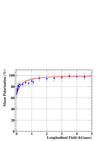
Figure 1: Muon residual polarization after the muons stop in a polyethylene target, as a function of the external magnetic field (adapted from Buhler2 ).

So, we can assume that even in our case the strong magnetic field quenches any depolarizing effect.

The last point to be addressed is that muons reach the target centre under different angles within a $\approx 1\times 1\leavevmode\nobreak\ {\rm cm}^{2}$ beam spot. This angular spread corresponds to an apparent depolarization, since $P_{\mu}$ does not coincide with $P^{z}_{\mu}$. Using the full MEG Monte Carlo (MC) simulation we evaluated that the angular divergence at the target corresponds to a cone of $<20^{\circ}$ opening angle, corresponding to $\approx 3\leavevmode\nobreak\ \%$ apparent depolarization.

2.4 Total depolarization

In conclusion, the main depolarizing effects are due to cloud muons and beam divergence. The average final polarization along the beam axis ($z$) is:

$$\langle P^{z}_{\mu}\rangle=\left(-0.91\pm 0.03\right),$$ (5)

where the systematic uncertainty takes into account the uncertainties in this computation. The various contributions are listed in Tab. 1.

Table 1: Summary of main depolarizing effects (%).

Source	(%)
Multiple scattering in the production target	0.3
Cloud muons	4.5
Muon transport along the beam line	0.8
Muon interactions with the MEG target	negligible
Muon angular spread at the target	3.0
Total	8.6

3 Expected Michel positron spectrum from polarized muons

The angular distribution of Michel positrons was calculated in detail by several authors including the effect of the electron mass and the first order radiative corrections kuno_2001 ; kinoshita_1959 ; Arbuzov:2001ui . The bidimensional energy-angular distribution for polarized $\mu^{+}$ decaying at rest, neglecting the electron mass, takes the following form:

$$\frac{d^{2}\Gamma\left(\mu^{+}\rightarrow{\rm e}^{+}\nu\bar{\nu}\right)}{dxd\cos\theta_{\rm e}}=\frac{{m_{\mu}}^{5}{G_{F}}^{2}}{192{\pi}^{3}}$$

$$x^{2}\left[F(x)+P_{\mu}\cos\theta_{\rm e}G(x)\right]$$

$$F(x) =f_{0}(x)+\frac{\alpha}{2\pi}f_{1}(x)+{\cal O}(\alpha^{2})$$

$$G(x) =g_{0}(x)+\frac{\alpha}{2\pi}g_{1}(x)+{\cal O}(\alpha^{2})$$

$$f_{0}(x) = \left(3-2x\right)\qquad g_{0}(x)=\left(2x-1\right)$$ (6)

where $P_{\mu}$ is the $\mu^{+}$ polarization along a selected axis, $x=2E_{{\rm e}^{+}}/m_{\mu}$ ($0\leq x\leq 1$) and $\theta_{\rm e}$ is the angle formed by the positron momentum vector and the polarization axis. Expressions for $f_{1}(x)$ and $g_{1}(x)$ neglecting the electron mass are available in kinoshita_1959 ; the MC simulations in the following are based on Eq. 6 including first order radiative corrections and neglecting the electron mass. Formulae incorporating the dependence on electron mass for all terms in Eq. 6 are presented in Arbuzov:2001ui .
We show in Fig. 2 the angular distribution from Eq. 6 in the range $60^{\circ}\div 120^{\circ}$ for different values of $x$.

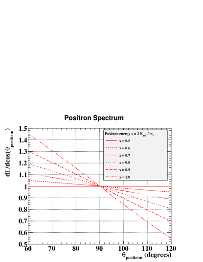
Figure 2: Angular distributions of Michel positrons referred to the $\mu^{+}$ spin direction for six different values of $x$, as given by Eq. 6. The vertical scale is in arbitrary units and normalized to $1$ for $\theta_{\rm e}=90^{\circ}$.

The differential decay width for $x=1$ at $\theta_{\rm e}=70^{\circ}$ is about twice that at $\theta_{\rm e}=110^{\circ}$. Inspection of Fig. 2 shows that detectable effects are expected in the MEG data sample, even if the MEG apparatus is not the best suited for polarization measurements due to the relatively small angular range, centred around $\theta_{\rm e}=90^{\circ}$.

4 Results of the measurement

4.1 Generalities

In the previous section we showed that polarization effects can be observed in the angular distributions of high-energy positrons from Michel decays. In addition to that, the distribution of high-energy photons from Radiative Muon Decay (RMD) is expected to be affected by the polarization; however its associated error is very large, because of the intrinsic uncertainties in the analysis method, mainly related to the determination of the photon emission angle, and because of the presence in this data sample of a large background of photons from other sources (e.g. bremsstrahlung, annihilation in flight, pile-up of lower energy gamma’s …). We will therefore disregard this item.

It is important to note that in Eq. 6 the quantization axis is the muon spin direction; however, surface muons are expected to be fully polarized in the backward direction, i.e. along the negative $z$-axis. Therefore, the polar angle $\theta$ in the MEG reference frame is related to $\theta_{\rm e}$ in Eq. 6 by $\theta=180^{\circ}-\theta_{\rm e}$. Hence, the excess in the theoretical angular distribution Eq. 6 for $\theta_{\rm e}<90^{\circ}$ corresponds to an excess for $\theta>90^{\circ}$ in the experimental angular distribution, i.e. on the US-side.

A very powerful way to study the muon polarization is to compare the energy spectra, integrated over the angular acceptance, on the US ($\left(dN/dE_{\rm e^{+}}\right)_{US}$) and on the DS ($\left(dN/dE_{\rm e^{+}}\right)_{DS}$) sides. In Fig. 3 we show the expected asymmetry between $45\leavevmode\nobreak\ {\rm MeV}$ and $53\leavevmode\nobreak\ {\rm MeV}$ as a function of positron energy $E_{\rm e^{+}}$ :

$$A\left(E_{\rm e^{+}}\right)=\frac{\left(\left(dN/dE_{\rm e^{+}}\right)_{US}-\left(dN/dE_{\rm e^{+}}\right)_{DS}\right)}{\left(\left(dN/dE_{\rm e^{+}}\right)_{US}+\left(dN/dE_{\rm e^{+}}\right)_{DS}\right)}$$ (7)

in the upper part and the ratio:

$$R\left(E_{\rm e^{+}}\right)=\frac{\left(dN/dE_{\rm e^{+}}\right)_{US}}{\left(dN/dE_{\rm e^{+}}\right)_{DS}}$$ (8)

in the lower part for three representative polarization values: $0$ (red dotted line), $-0.5$ (black dashed line) and $-1$ (blue continuous line). First order R.C. are taken into account and have a $\approx 0.3\,\%$ effect on both asymmetry and ratio.

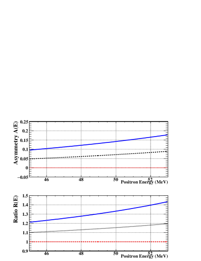
Figure 3: The asymmetry (7) (upper plot) and the ratio (8) (lower plot) as a function of the positron energy $E_{\rm e^{+}}$, for three representative polarization values: $0$ (red dotted line), $-0.5$ (black dashed line) and $-1$ (blue continuous line). All spectra are obtained by integrating the 2-D (energy, angle) distributions over the MEG angular range. The contribution of first order R.C. on both asymmetry and ratio is $\approx 0.3\,\%$ while those of higher order corrections and of neglecting the electron mass are even smaller.

4.2 Analysis of Michel positrons

Experimentally measured angular distributions are a result of the convolution of the expected theoretical distributions with the detector response, acceptance and thresholds, whose non-uniformities can mimic angular asymmetries or create fictitious ones. Topological requirements and quality cuts needed to define and fit charged particle tracks also introduce angle-dependent non-uniformities. In particular, the tracking algorithm has a lower efficiency for positrons emitted with small longitudinal momenta, resulting in a dip in the angular distribution of Michel positrons for $\theta\approx 90^{\circ}$ (see later Fig. 7). MEG positrons are mainly produced by muon decays in the stopping target, with a significant fraction ($\sim 20\leavevmode\nobreak\ \%$) decaying off-target, in beam elements or in the surrounding helium gas. However, this contribution can be minimized by requiring the reconstructed positron decay vertex to lie within the target volume. The fraction of the positrons decaying off-target and reconstructed on the target was evaluated by a complete MC simulation of the muon trajectory along the PSI/MEG beam line up to the stopping target and of the subsequent muon decay. This fraction was found to be smaller than 0.5% and can be considered as a source of systematic uncertainty assuming, very conservatively, the same effect on the polarization measurement. In summary, an analytical prediction of the experimental distribution is rather complicated; hence, we decided to measure the muon polarization by means of two different analysis strategies:

• in the first one, we compared the energy integrated experimental angular distribution of Michel positrons with that obtained by a detailed Geant3-based MC simulation of those events, as seen in the MEG detector, with the muon polarization as a free input parameter;

• in the second one, we measured the US-DS asymmetry $A\left(E_{\rm e^{+}}\right)$ and the ratio $R\left(E_{\rm e^{+}}\right)$ as a function of positron energy and fit them with the expected phenomenological forms, after unfolding the detector acceptance and response.

4.2.1 MC simulation

The MEG MC simulation is described in details in meg2009 and softwaretns . Michel positrons were generated in the stopping target (the full simulation of the muon beam up to the stopping target described above was not used since it is much slower and does not bring significant advantages in this case) with a minimum energy of $40\leavevmode\nobreak\ {\rm MeV}$ and a muon polarization $P_{\mu}$ varying between $0$ and $-1$ in steps of $0.1$. A smaller step size of $0.05$ was used between $-0.8$ and $-1$, close to the expected value (section 2). Separate samples of MC events were produced for each polarization value and the positron energy and direction were generated according to the theoretical energy-angle distribution corresponding to this polarization. Positrons were individually followed within the fiducial volume and their hits in the tracking system and on the timing counters were recorded; a simulation of the electronic chain converted these hits into anodic and cathodic signals which were processed by the same analysis algorithms used for real data. Modifications of the apparatus configuration during the whole period of data taking were simulated in detail, following the information recorded for each run in the experiment database. The position and spatial orientation of the target varied slightly each year, as well as trigger and acquisition thresholds, beam spot centre and size and the drift chamber alignment calibration constants. Some of the drift chambers suffered from instabilities, with a time scale from days to weeks, with their supply voltages finally set to a value smaller than nominal. The supply voltage variations, chamber by chamber, were also followed in the simulation on a run by run basis. However, voltage instabilities do not significantly affect the polarization measurement. Since drift chamber wires run along the $z$-axis, a non operating chamber produces the same effect on US and DS if the beam is perfectly centred on the target, while it gives a second order contribution to the US-DS asymmetry when the beam is not perfectly centred. The number of MC events generated using the global configuration (target position, alignment …) corresponding to a given year is proportional to the actual amount of data collected in that year.

4.2.2 Data sample

The data sample contains the events collected between $2009$ and $2011$ by a pre-scaled trigger requiring only a timing counter hit above the threshold (so called “trigger 22”). The analysis procedure requires an accurate pre-selection of good quality tracks: strict selection cuts are applied in order to single out tracks with good angular and momentum resolutions, well matched with at least one timing counter hit and with the decay vertex reconstructed within the target volume. A fiducial volume cut is included to avoid efficiency distorsions at the borders of the acceptance. The sample and the selection criteria are essentially those used to identify Michel events for the absolute normalization of the MEG data (see meg2010 ; meg2013 ). About $37k$ ($2009$), $65k$ ($2010$) and $115k$ ($2011$) positron tracks passed all selection cuts, for a total of about $2.1\times 10^{5}$ events. The same criteria were applied to the MC tracks; about $1.3\times 10^{5}$ events passed all selections for each polarization value.

4.2.3 Comparison between MC and data

The comparisons between the reconstructed positron vertex coordinates $x$, $y$ and $z$ for data (blue points) and MC (red line, normalized to the data) are shown in Fig. 4, top and bottom left; at the bottom right the same comparison for the reconstructed azimuthal angle $\phi$ at the positron emission point is shown.

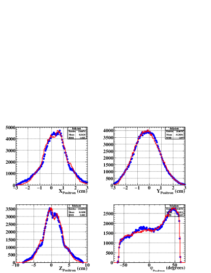
Figure 4: Comparison between the reconstructed vertex coordinates $x$, $y$ and $z$ and the azimuthal $\phi$ angle, for real (blue points) and simulated data (red line, normalized to the data). The polarization of the MC sample is $-0.85$; the distributions corresponding to different polarizations are almost identical.

We also show in Fig. 5 the comparison between data (blue points) and MC (red line) positron energy spectra on the US (left) and DS (right) sides. In the upper part of the figure we report the superimposed data and MC distributions, while in the lower part we show the ratios data/MC as a function of the positron energy (in ${\rm MeV}$). All spectra are corrected for the left-right correction factors which will be discussed in the next section.

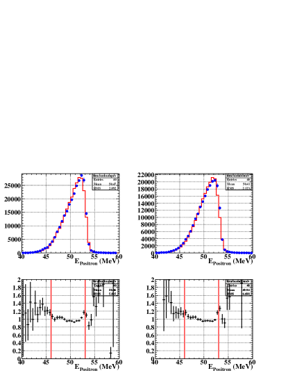
Figure 5: Upper plots: comparison between data (blue points) and MC (red line, normalized to the data) positron energy spectra for the US (left) and DS (right) sides. Lower plots: ratio data/MC as a function of positron energy for US (left) and DS (right) sides. The red vertical lines indicate the boundaries of the fitting region ($46\leavevmode\nobreak\ {\rm MeV}<E<53\leavevmode\nobreak\ {\rm MeV}$)

.

The red vertical lines in the bottom plots define the energy region where the polarization fit is performed ($46\leavevmode\nobreak\ {\rm MeV}<E<53\leavevmode\nobreak\ {\rm MeV}$). The agreement between data and MC is generally quite good for the spatial coordinates, while some ($<10\,\%$) discrepancies can be observed in the energy spectra and expecially in their ratios, even in the fit region. Data/MC ratios are consistent with unity for $48\leavevmode\nobreak\ {\rm MeV}<E<52\leavevmode\nobreak\ {\rm MeV}$, but exhibit some systematic differences close to the threshold ($E\approx 45-48\leavevmode\nobreak\ {\rm MeV}$) and in the upper edge ($E>52\leavevmode\nobreak\ {\rm MeV}$). Such discrepancies are due to the fact that the MC simulation is not able to perfectly reproduce the experimental energy resolution: for instance $\sigma_{E}\approx 340\leavevmode\nobreak\ {\rm keV}$ for data and $\approx 260\leavevmode\nobreak\ {\rm keV}$ for MC at $E=52.83\leavevmode\nobreak\ {\rm MeV}$. However, if one looks at both bottom plots together, one sees that the differences are clearly correlated; then, they tend to cancel out when one uses $A\left(E_{\rm e^{+}}\right)$ or $R\left(E_{\rm e^{+}}\right)$ as analysis tools. We also note that the differences are particularly relevant in the year $2010$ sample, when the beam centre was displaced with respect to the target centre by some ${\rm mm}$. (See section 4.2.7 dedicated to the analysis of systematic uncertainties.)

The general agreement between data and MC for all reconstructed variables demonstrates our ability to correctly simulate the behaviour of the apparatus.

4.2.4 Efficiency correction for MC and data

The efficiency for the full reconstruction of a positron event is composed of two parts: the absolute efficiency $\epsilon(Track)$ for producing a track satisfying all trigger and software requirements and the relative efficiency $\epsilon\left(TC\left|Track\right.\right)$ of having a TC hit, given a track. Both efficiencies are functions of the positron energy and emission angles and can be different on the US and DS sides because of intrinsic asymmetries of the experimental apparatus.

The $\epsilon\left(TC\left|Track\right.\right)$ efficiency was separately computed for MC and real events. In the case of MC this calculation is straightforward. In the more complicate case of real data, we selected positrons collected by a different pre-scaled trigger (so called “trigger 18”) requiring only loose conditions on the number and the topological sequence of fired drift chambers, and selected the fraction of tracks with an associated good TC hit within this sample. The MC and data $\epsilon\left(TC\left|Track\right.\right)$ efficiency matrices were then used to correct the $\theta$ angular distributions, $A\left(E_{\rm e^{+}}\right)$ and $R\left(E_{\rm e^{+}}\right)$.

The $\epsilon(Track)$ efficiency was extracted from MC by looking at the reconstructed $R\left(E\right)$ in the MC sample generated with $P_{\mu}=0$ and determining, year by year, an empirical correction function which makes this $R\left(E\right)$ always consistent with unity within the errors. We show in Fig. 6 the correction functions for $2009$ (red), $2010$ (black) and $2011$ (blue) samples.

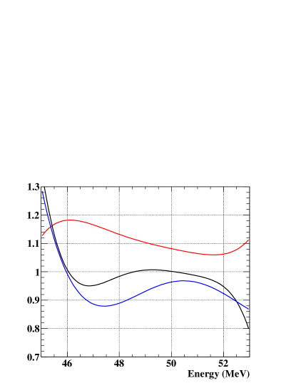
Figure 6: Empirical correction functions applied to make the ratio $R\left(E_{\rm e^{+}}\right)$ for MC events generated with null polarization consistent with unity. The red line is for $2009$, the black one for $2010$ and the blue line for $2011$ sample.

We then applied the same correction functions to all MC samples and we checked that the polarization values extracted by fitting $A\left(E_{\rm e^{+}}\right)$ and $R\left(E_{\rm e^{+}}\right)$ were consistent with those generated. The correction functions were also applied to the data since the good agreement between MC and data shown in Fig. 4 and 5 gives us confidence of the correct apparatus response to positron events.

4.2.5 Results of first strategy: angular distribution

In Fig. 7 the comparison between the angular distributions of real data (blue points) and of MC events (red line, normalized to the data), after inserting the matching efficiency corrections, as a function of $\theta$ angle for two different polarization values is shown: $P_{\mu}=0$ in the upper plot and $P_{\mu}=-0.85$ in the lower plot.

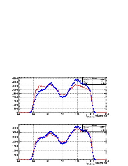
Figure 7: Comparison between the angular distributions for simulated (red line) and measured (blue points) Michel positrons; $P_{\mu}=0$ (upper plot) and $P_{\mu}=-0.85$ (lower plot). The polar angle $\theta$ is referred to the beam axis. Histograms are normalized to the data.

According to Eq. 6 and to the definition of $\theta$, we expect to observe an asymmetric distribution for large values of the polarization, with an excess on the US-side ($\theta>90^{\circ}$) and a symmetric distribution for null polarization. Fig. 7 shows a clear disagreement between data and MC for $P_{\mu}=0$ and a good agreement for $P_{\mu}=-0.85$. The simulation well reproduces the US-DS asymmetry observed in the data, as well as the dip for $\theta\approx 90^{\circ}$. Angular distributions for $P_{\mu}=-0.8$ and for $P_{\mu}=-0.9$ do not significantly differ from that shown for $P_{\mu}=-0.85$: the comparison between data and MC gives strong indications for a large polarization, $-\left(0.8-0.9\right)$, but it is not precise enough to single out a value of $P_{\mu}$, with its uncertainty.

4.2.6 Results of second strategy: US-DS asymmetry and ratio

A quantitative estimate of the polarization can be obtained by studying the angle-integrated energy distributions $\left(dN/dE\right)_{US}$ and $\left(dN/dE\right)_{DS}$ on the US and DS sides. Eq. 6 shows that the difference between the US and DS sides is due to the presence of a term proportional to $xP_{\mu}\cos\theta$. Since the sign of this term changes from US (where, according to our definition of polar angles, it is positive) to DS (where, with the same definition, it is negative), one expects that both the asymmetry $A\left(E_{\rm e^{+}}\right)$ and the ratio $R\left(E_{\rm e^{+}}\right)$ increase almost linearly with the positron energy. The slope of this dependence is $P_{\mu}\cos\theta$: one can therefore extract a polarization value by fitting the experimentally measured asymmetry and ratio and dividing the measured slope by the average value of $\langle\left|\cos\theta\right|\rangle=0.1762$ for the US and DS sections. However, since the angular acceptance is correlated with the energy, the averarge value of $\cos\theta$ is a function $\langle\cos\theta\left(E\right)\rangle$, which can be extracted directly from the data. Then, we replaced in the fitting formula the energy averaged value $\langle\left|\cos\theta\right|\rangle$ with $\langle\cos\theta\left(E\right)\rangle$, bin by bin (the differences between the energy dependent values and the energy averaged one are at $\pm 5\,\%$ level). The fit interval was restricted to $\left(46-53\right)\leavevmode\nobreak\ {\rm MeV}$ to minimize possible distorsions due to the energy-angle dependencies of the energy threshold and because Eq. 6 is meaningless for $E>52.83\leavevmode\nobreak\ {\rm MeV}$, i.e. $x>1$. The expected plots for $A\left(E_{\rm e^{+}}\right)$ and $R\left(E_{\rm e^{+}}\right)$ are shown in Fig. 3. The experimental $A\left(E_{\rm e^{+}}\right)$ and $R\left(E_{\rm e^{+}}\right)$ were separately determined year by year and summed. The fit results for the full data sample are shown in Fig. 8; the average value of the two fits is

$$P_{\mu}=-0.856\pm 0.021,$$ (9)

where the quoted error is only statistical.

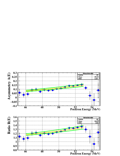
Figure 8: Fit of $A\left(E_{\rm e^{+}}\right)$ (upper plot) and of $R\left(E_{\rm e^{+}}\right)$ (lower plot) as a function of the positron energy. The experimental data are corrected, year by year, by the MC-based tracking efficiency functions and the fitting function for the $\langle\cos\theta\left(E\right)\rangle$ dependence. The green lines represent the $\pm 1\leavevmode\nobreak\ \sigma$ band, including both the statistic and the systematic uncertainties. The fitting functions are obtained from the distribution in Eq. 6.

The average $\chi^{2}/d.o.f.$ of the fits is $0.74$, mainly determined by the points close to the threshold. In both plots the yellow line represents the best fit, while the two green lines show the $\pm 1\leavevmode\nobreak\ \sigma$ band, obtained by adding or subtracting the sum of statistic and systematic uncertainties (see next section for the discussion of systematic uncertainties).

If we fit the polarization values year by year we obtain the results reported in Tab. 2, where again the quoted errors are only statistical.

Table 2: Results of the polarization fit year by year.

	$2009$	$2010$	$2011$	Global
$\langle P\rangle\pm\Delta P$	$0.85\pm 0.05$	$0.71\pm 0.05$	$0.92\pm 0.04$	$0.856\pm 0.021$
$\chi^{2}$/d.o.f.	$0.90$	$1.37$	$0.34$	$0.74$

The polarization value measured in $2010$ sample is significantly lower than in the other two years; however, the larger values of the $\chi^{2}$/d.o.f. suggests that this result is of lower quality and less reliable. The observed deviation in $2010$ data is discussed in the next section and is reflected in the associated systematic error.

In Fig. 9 we show the comparison between data (blue filled points) and MC generated with $P_{\mu}=-0.85$ (red open triangles) for $A\left(E_{\rm e^{+}}\right)$ (upper plot) and $R\left(E_{\rm e^{+}}\right)$ (lower plot) between $45$ and $55\leavevmode\nobreak\ {\rm MeV}$: the agreement is quite good everywhere in the selected energy interval.

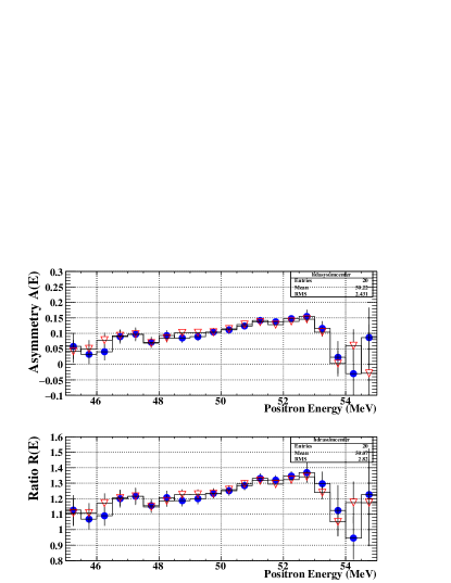
Figure 9: Comparison between data (blue filled points) and MC for $P_{\mu}=-0.85$ (red open triangles). $A\left(E_{\rm e^{+}}\right)$ (upper plot) and $R\left(E_{\rm e^{+}}\right)$ (lower plot) between $45$ and $55\leavevmode\nobreak\ {\rm MeV}$.

Note that the energy region above $53\leavevmode\nobreak\ {\rm MeV}$, where the data and MC errors are quite large, does not affect the result, since the fit was limited to $\left(46-53\right)\leavevmode\nobreak\ {\rm MeV}$. We checked that these results do not depend on the fitting interval by eliminating one bin at the lower bound and/or one bin at the upper bound: in all cases the fit results agreed with (9) within the statistical error.

4.2.7 Systematic uncertainties

Various systematic uncertainties can produce sizable effects on this measurement. We single out seven main possible sources: energy scale, angular bias, target position, MC-based efficiency corrections, threshold effects, higher order corrections, including the effect of finite electron mass, in the theoretical calculations and off-target muon decays. The first three affect the shape of the spectra on the US and DS sides and the evaluation of the relative efficiency $\epsilon\left(TC\left|Track\right.\right)$ from data; the fourth determines the absolute tracking efficiency; the fifth can alter the $A\left(E_{\rm e^{+}}\right)$ and $R\left(E_{\rm e^{+}}\right)$ fits in the bins close to the lower bound of the fit interval, the sixth can modifiy the fitting function and the seventh can alter the quality of the selected positron sample.

• Energy scale. The energy scale and resolution are determined in MEG, as discussed in meg2010 , by fitting the Michel positron energy spectrum with the convolution of the theoretical spectrum (including radiative corrections) of the detector acceptance and of a resolution curve, in the form of a partially constrained triple Gaussian shape. The position of the Michel edge, used as a reference calibration point, is determined with a precision of $\delta E_{\rm e^{+}}\sim 30\leavevmode\nobreak\ \leavevmode\nobreak\ {\rm keV}$. The effect of this uncertainty was evaluated by varying the reconstructed energy of our events by a factor $\left(1\pm\delta E_{\rm e^{+}}/\bar{E}_{\rm e^{+}}\right)$, where $\bar{E}_{\rm e^{+}}=52.83\leavevmode\nobreak\ {\rm MeV}$ is the position of the Michel edge, and repeating the analysis. The polarization value determined by the average of $A\left(E_{\rm e^{+}}\right)$ and $R\left(E_{\rm e^{+}}\right)$ fits increases by $0.0029$ when $\delta E_{\rm e^{+}}/\bar{E}_{\rm e^{+}}$ is added and decreases by $-0.0052$ when $\delta E_{\rm e^{+}}/\bar{E}_{\rm e^{+}}$ is subtracted.

• Angular bias. The angular resolution is determined by looking at tracks crossing the chamber system twice (double turn method), as discussed in meg2009 ; meg2010 . The uncertainty on the $\theta$ and $\phi$ scales varies between $1$ and $3\leavevmode\nobreak\ {\rm mrad}$. The effect of this uncertainty on the angular scale was (conservatively) evaluated by modifying both the reconstructed polar angles by $\pm 3\leavevmode\nobreak\ {\rm mrad}$ and repeating the analysis. The measured polarization decreases (increases) by $-0.013$ ($+0.025$).

• Target position. The target position with respect to the centre of the COBRA magnet is measured by means of an optical survey and checked by looking at the distribution of the positron vertex of reconstructed tracks. The discrepancies between the two methods are at the level of a fraction of a mm. Since in our analysis we require that the reconstructed positron vertex lies within the target ellipse, an error on the target position can alter the positron selection. We assumed a conservative estimate of a target position uncertainty of $\pm 1\leavevmode\nobreak\ {\rm mm}$ on all coordinates and, as previously, added or subtracted it and repeated the analysis. The effect was to decrease (increase) the polarization by $-0.022$ ($0.016$).

• MC-based corrections. The MC corrections, inserted to take into account the absolute tracking efficiency, are based on the position of the target as measured by the optical survey and on the nominal location of the beam centre. A variation of these parameters produces a variation on the correction functions, applied year by year to MC and data. We estimated the size of this effect by generating MC samples with a displaced beam and target ($\pm 1\leavevmode\nobreak\ {\rm mm}$ shift as previously) and null polarization and determined new tracking efficiency correction functions. Such functions were then applied to the data and MC: the measured polarization decreased (increased) by $-0.035$ ($0.036$).

• Threshold effects. The response of the MEG tracking system close to the momentum threshold ($E_{\rm e^{+}}\approx 45\leavevmode\nobreak\ {\rm MeV}$) depends in general on the polar angles and can be significantly distorted when the beam and target are not centred, causing fictitious differences between the US and DS sides. In 2010 the beam centre to target centre displacement was maximal, corresponding to more than $3\leavevmode\nobreak\ {\rm mm}$ in the horizontal plane and just over $3\leavevmode\nobreak\ {\rm mm}$ in the vertical plane, producing an asymmetric US-DS energy threshold, with the DS spectrum systematically higher than the US one for $E_{\rm e^{+}}<47\leavevmode\nobreak\ {\rm MeV}$. The beam and target displacement were introduced in the MC, but the simulation for $2010$ did not result in a good agreement with the data in the region close to the energy threshold. We then estimated the systematic effect due to the angular dependence of the energy threshold by removing the $2010$ sample from the fit: the polarization decreases by $-0.047$, a difference twice larger than the statistical error. The $\chi^{2}/d.o.f.$ of the fit improved a bit from $0.74$ to $0.71$. A better fit quality was observed also on MC events by removing the simulated data corresponding to the year $2010$ configuration.

• Higher order corrections to the theoretical formula in Eq. 6. The effect of second and higher order contributions and of taking into account the finite electron mass to the muon decay rate is discussed in some detail in Arbuzov:2002cn ; Arbuzov:2002pp ; Arbuzov:2002rp ; Arbuzov:2004wr . The conclusion is that they are smaller than the first order correction and therefore we can deduce that the effect of including them in Eq. 6 for extracting the polarization from Fig. 8 is not larger than the effect of the first order correction that is 0.3%. Hence this value can be assumed as a conservative estimation of the systematic error due to higher order corrections.

• Off-target muon decays. A conservative estimation of off-target muon decays as discussed in Sect. 4.2 is 0.5%, that is 0.004 on the polarization value.

The effects of the various systematic uncertainties and the global systematic uncertainty calculated by their addition in quadrature are reported in Tab.3.

Table 3: Main systematic uncertainties and their effect on polarization.

Source	($\Delta P$)
Energy scale	$\left(+0.0029,-0.0052\right)$
Angular scale	$\left(+0.025,-0.013\right)$
Target position	$\left(+0.016,-0.022\right)$
Tracking efficiency	$\left(+0.036,-0.035\right)$
Energy threshold	$-0.047$
Higher order corrections	$\pm 0.003$
Off-target decsy	$\pm 0.004$
Total (in quadrature)	$\left(+0.047,-0.064\right)$

Combining the fit results in (9) with the numbers reported in Tab.3 we can state that the muon residual polarization in the MEG experiment is:

$$P_{\mu}=-0.86\pm 0.02\leavevmode\nobreak\ {\rm(stat)}\leavevmode\nobreak\ {}^{+0.05}_{-0.06}\leavevmode\nobreak\ {\rm(syst)}.$$ (10)

5 Summary and conclusions

We measured the residual muon polarization $P_{\mu}$ in the MEG experiment by studying the energy-angle distribution of Michel positrons collected during three years of data taking. We obtained:

$$P_{\mu}=-0.86\pm 0.02\leavevmode\nobreak\ {\rm(stat)}\leavevmode\nobreak\ {}^{+0.05}_{-0.06}\leavevmode\nobreak\ {\rm(syst)}.$$ (11)

The measured value is in agreement with the value expected from calculation of the depolarizing effects due to the muon spin interactions during the production and the propagation through the apparatus up to the stopping target, based on the SM prediction of positive surface muons, produced fully polarized in the direction opposite to the beam direction. Moreover, the Michel positron angular distribution and the US - DS asymmetry of the positron energy spectra are well reproduced by a complete simulation of the positron detection in the MEG set-up when a muon polarization $P_{\mu}=-0.85$ is used as an input parameter in the MC calculation. This result is important to allow a precise calculation of the Radiative Muon Decay branching ratio and energy-angle distribution in the kinematic region where it represents a background source to the search for ${\mu^{+}\to e^{+}\gamma}$ and can be used as a tool for the absolute normalization of the MEG experiment.

6 Acknowledgements

We are grateful for the support and cooperation provided by PSI as the host laboratory and to the technical and engineering staff of our institutes. This work is supported by SNF grant 200021_137738 (CH), DOE DEFG02-91ER40679 (USA), INFN (Italy) and MEXT KAKENHI 22000004 and 26000004 (Japan). Partial support of the Italian Ministry of University and Research (MIUR) grant RBFR08XWGN, Ministry of University and Education of the Russian Federation and Russian Fund for Basic Research grants RFBR 14-22-03071 are acknowledged.

References

- [1] aea.web.psi.ch/beam2lines/beampie5.html.
- [2] J. Adam et al. The MEG detector for decay search. Eur. Phys. J. C, 73:2365, 2013.
- [3] https://www.psi.ch.
- [4] J. Adam et al. A limit for the decay from the MEG experiment. Nucl. Phys., B834:1–12, 2010.
- [5] J. Adam et al. New limit on the lepton-flavor violating decay . Phys. Rev. Lett., 107:171801, 2011.
- [6] J. Adam et al. New constraint on the existence of the decay. Phys. Rev. Lett., 110:201801, 2013.
- [7] A. Yamamoto et al. A thin superconducting solenoid magnet for particle physics. Appl. Supercond., IEEE Trans. on, 12:438–441, 2002.
- [8] W. Ootani, W. Odashima, S. Kimura, T. Kobayashi, Y. Makida, T. Mitsuhashi, S. Mizumaki, R. Ruber, and A. Yamamoto. Development of a thin-wall superconducting magnet for the positron spectrometer in the MEG experiment. Appl. Supercond., IEEE Trans. on, 14(2):568–571, June 2004.
- [9] M. Hildebrandt. The drift chamber system of the MEG experiment. Nucl. Instr. Methods Phys. Res., Sect. A, 623(1):111 – 113, 2010.
- [10] S. Dussoni and M. De Gerone and F. Gatti and R. Valle and M. Rossella and R. Nardó and P.W. Cattaneo. The Timing Counter of the MEG experiment: design and commissioning. Nucl. Instr. Methods Phys. Res., Sect. A, 617(1-3):387 – 390, 2010.
- [11] M. De Gerone, S. Dussoni, K. Fratini, F. Gatti, R. Valle, et al. Development and commissioning of the Timing Counter for the MEG Experiment. IEEE Trans. Nucl. Sci., 59:379–388, 2012.
- [12] M. De Gerone, S. Dussoni, K. Fratini, F. Gatti, R. Valle, et al. The MEG timing counter calibration and performance. Nucl.Instrum.Meth., A638:41–46, 2011.
- [13] R. Sawada. Performance of liquid xenon gamma ray detector for MEG. Nucl. Instr. Methods Phys. Res., Sect. A, 623(1):258 – 260, 2010.
- [14] Satoshi Mihara. MEG liquid xenon detector. J.Phys.Conf.Ser., 308:012009, 2011.
- [15] L. Galli, F. Cei, S. Galeotti, Magazzù C., D. Nicolò, G. Signorelli, and M. Grassi. An FPGA-based trigger system for the search of decay in the MEG experiment. J. Instrum., 8:P01008, 2013.
- [16] L. Galli, A. Baldini, P.W. Cattaneo, F. Cei, M. De Gerone, S. Dussoni, et al. Operation and performance of the trigger system of the MEG experiment. J. Instrum., 9:P04022, 2014.
- [17] S. Ritt. The DRS chip: cheap waveform digitizing in the GHz range. Nucl. Instr. Methods Phys. Res., Sect. A, 518(1-2):470–471, Feb 2004.
- [18] S. Ritt, R. Dinapoli, and U. Hartmann. Application of the DRS chip for fast waveform digitizing. Nucl. Instr. Methods Phys. Res., Sect. A, 623(1):486 – 488, 2010.
- [19] A. Baldini et al. A radioactive point-source lattice for calibrating and monitoring the liquid xenon calorimeter of the MEG experiment. Nucl. Instr. Methods Phys. Res., Sect. A, 565(2):589 – 598, 2006.
- [20] J. Adam et al. Calibration and monitoring of the MEG experiment by a proton beam from a Cockcroft–Walton accelerator. Nucl. Instr. Methods Phys. Res., Sect. A, 641:19–32, 2011.
- [21] A. Papa. Search for the lepton flavour violation in . The calibration methods for the MEG experiment PhD thesis, University of Pisa, 2010, Edizioni ETS.
- [22] A. E. Pifer. A high stopping density beam. Nucl. Instr. Methods Phys. Res., Sect. A, 135:39–46, 1976.
- [23] O.B. Van Dyck, E.W. Hoffman, R.J. Macek, G. Sanders, R.D. Werbeck, et al. ’Cloud’ and ’surface’ muon beam characteristics. IEEE Trans.Nucl.Sci., 26:3197–3199, 1979.
- [24] J. D. Jackson. Classical Electrodynamics. Wiley & Sons, 1998.
- [25] Brewer J. H., others in Hughes V. W., and C.S. Wu. Muon Physics, chapter vol III and I. Academic Press, New York, 1975.
- [26] R. A. Swanson. Depolarization of positive muons in condensed matter. Phys. Rev., 112(2):580–586, 1958.
- [27] A. Buhler et al. Measurements of muon depolarization in several materials. Nuovo Cimento, 39:824, 1965.
- [28] A. Buhler et al. Study of the quenching of muon depolarization in several materials as a function of externally applied magnetic fields. Nuovo Cimento, 39:812, 1965.
- [29] Y. Kuno and Y. Okada. Muon decay and physics beyond the standard model. Rev. Mod. Phys., 73(1):151–202, 2001.
- [30] T. Kinoshita and A. Sirlin. Radiative corrections to Fermi interactions. Phys. Rev., 113(6):1652–1660, 1959.
- [31] A.B. Arbuzov. First order radiative corrections to polarized muon decay spectrum. Phys. Lett., B524:99–106, 2002.
- [32] P.W. Cattaneo, F. Cei, R. Sawada, M. Schneebeli, and S. Yamada. The architecture of MEG simulation and analysis software. Eur. Phys. J. Plus, 126(7):1–12, 2011.
- [33] A.B. Arbuzov and K. Melnikov. O(alpha**2 ln(m(mu) / m(e)) corrections to electron energy spectrum in muon decay. Phys. Rev., D66:093003, 2002.
- [34] A.B. Arbuzov, A. Czarnecki, and A. Gaponenko. Muon decay spectrum: Leading logarithmic approximation. Phys. Rev., D65:113006, 2002.
- [35] A.B. Arbuzov. Higher order QED corrections to muon decay spectrum. JHEP, 03:063, 2003.
- [36] A.B. Arbuzov and E.S. Scherbakova. One-loop corrections to radiative muon decay. Phys. Lett., B597:285–290, 2004.