The asymptotics of the Struve function ${\bf H}_{\nu}(z)$ for large complex order and argument

Abstract

We re-examine the asymptotic expansion of the Struve function ${\bf H}_{\nu}(z)$ for large complex values of $\nu$ and $z$ satisfying $|\arg\,\nu|\leq\leavevmode\hbox{${\textstyle\frac{1}{2}}$}\pi$ and $|\arg\,z|<\leavevmode\hbox{${\textstyle\frac{1}{2}}$}\pi$. Watson’s analysis [4, §10.43] covers only the case of $\nu$ and $z$ of the same phase with $\nu/z$ in the intervals $(0,1)$ and $(1,\infty)$. The domains in the complex $\nu/z$-plane where the expansion takes on different forms are obtained.

Mathematics Subject Classification: 30E15, 33C10, 34E05, 41A60

Keywords: Struve function, asymptotic expansion, method of steepest descents

  

1.   Introduction

The Struve function ${\bf H}_{\nu}(z)$ is a particular solution of the inhomogeneous Bessel equation

$$\frac{d^{2}w(z)}{dz^{2}}+\frac{1}{z}\,\frac{dw(z)}{dz}+\biggl{(}1-\frac{\nu^{2}}{z^{2}}\biggr{)}\,w(z)=\frac{(\leavevmode\hbox{${\textstyle\frac{1}{2}}$}z)^{\nu-1}}{\surd\pi\,\Gamma(\nu+\leavevmode\hbox{${\textstyle\frac{1}{2}}$})}$$

which possesses the series expansion

$${\bf H}_{\nu}(z)=(\leavevmode\hbox{${\textstyle\frac{1}{2}}$}z)^{\nu+1}\sum_{n=0}^{\infty}\frac{(-)^{n}(\leavevmode\hbox{${\textstyle\frac{1}{2}}$}z)^{2n}}{\Gamma(n+\leavevmode\hbox{${\textstyle\frac{3}{2}}$})\Gamma(n+\nu+\leavevmode\hbox{${\textstyle\frac{3}{2}}$})}$$ (1.1)

valid for all finite $z$.

An integral representation, valid when $\Re(\nu)>-\leavevmode\hbox{${\textstyle\frac{1}{2}}$}$, is given by [4, p. 330] as

$$J_{\nu}(z)\pm i{\bf H}_{\nu}(z)=\frac{2(\leavevmode\hbox{${\textstyle\frac{1}{2}}$}z)^{\nu}}{\surd\pi\,\Gamma(\nu+\leavevmode\hbox{${\textstyle\frac{1}{2}}$})}\int_{0}^{1}e^{\pm izt}(1-t^{2})^{\nu-\frac{1}{2}}\,dt,$$

where $J_{\nu}(z)$ is the usual Bessel function. Upon replacement of the variable $t$ by $\pm iu$, we obtain

$${\bf H}_{\nu}(z)\pm iJ_{\nu}(z)=\frac{2(\leavevmode\hbox{${\textstyle\frac{1}{2}}$}z)^{\nu}}{\surd\pi\,\Gamma(\nu+\leavevmode\hbox{${\textstyle\frac{1}{2}}$})}\int_{0}^{\pm i}e^{-zu}(1+u^{2})^{\nu-\frac{1}{2}}\,du\quad(\Re(\nu)>-\leavevmode\hbox{${\textstyle\frac{1}{2}}$}).$$ (1.2)

The integration path corresponding to the upper sign in (1.2) can be deformed to pass along the positive real axis to $+\infty$ and back to the point $i$ along the parallel path $i+u$ ($0\leq u\leq\infty$). The contribution from the path $(i+\infty,i]$ is equal to $iH_{\nu}^{(2)}(z)$, where $H_{\nu}$ is the Hankel function; see [4, p. 166]. Thus we find the alternative representation [2, p. 292]

$${\bf H}_{\nu}(z)-Y_{\nu}(z)=\frac{2(\leavevmode\hbox{${\textstyle\frac{1}{2}}$}z)^{\nu}}{\surd\pi\,\Gamma(\nu+\leavevmode\hbox{${\textstyle\frac{1}{2}}$})}\int_{0}^{\infty}e^{-zu}(1+u^{2})^{\nu-\frac{1}{2}}\,du$$ (1.3)

valid for unrestricted $\nu$ and $|\arg\,z|<\leavevmode\hbox{${\textstyle\frac{1}{2}}$}\pi$, where $Y_{\nu}(z)$ denotes the Bessel function of the second kind.

Here we shall consider the asymptotic expansion of ${\bf H}_{\nu}(z)$ for large complex values of $\nu$ and $z$ satisfying $|\arg\,\nu|\leq\leavevmode\hbox{${\textstyle\frac{1}{2}}$}\pi$ and $|\arg\,z|<\leavevmode\hbox{${\textstyle\frac{1}{2}}$}\pi$. Values of $\arg\,z$ outside this range can be dealt with by means of the continuation formula

$${\bf H}_{\nu}(ze^{\pi mi})=e^{\pi mi(\nu+1)}\,{\bf H}_{\nu}(z),\qquad m=\pm 1,\pm 2\ldots$$

obtained from (1.1).

2.  Asymptotic expansion when $z>0$

We set

$$q:=\nu/z=\alpha+i\beta,\qquad\theta:=\arg\,z,\qquad\omega:=\arg\,q.$$

In view of (1.2) and (1.3), we are led to the consideration of the integral

$$\int_{C}e^{-|z|\tau}\frac{du}{\sqrt{1+u^{2}}}\qquad\tau:=e^{i\theta}\{u-q\log(1+u^{2})\},$$ (2.1)

where $C$ is a suitably chosen path in the $u$-plane.

Saddle points are situated at $d\tau/du=0$; that is, at the points

$$u_{\pm}=q\pm\sqrt{q^{2}-1}.$$

We shall refer to these saddles as $S_{1}$ (uuper sign) and $S_{2}$ (lower sign). Inversion of (2.1) in the form $u=\sum_{k=1}^{\infty}a_{k}(\tau e^{-i\theta})^{k}$, where $a_{0}=1$, shows that

$$\frac{1}{\sqrt{1+u^{2}}}\,\frac{du}{d\tau}=e^{-i\theta}\sum_{k=0}^{\infty}c_{k}(q)(\tau e^{-i\theta})^{k}$$

valid in a disc centered at $\tau=0$ of radius determined by the nearest singularity corresponding to the saddles $S_{1}$ or $S_{2}$ (or both). The values of the coefficients $c_{k}(q)$ ($0\leq k\leq 10$) are listed in Table 1; see also [1, p. 203].

Watson [4, §10.43] has considered the two cases (i) $q\in[1,\infty)$ and (ii) $q\in(0,1)$ when $z>0$ ($\theta=0$). The steepest descent paths emanating from the origin in the complex $u$-plane in these two cases are shown in Fig. 1; branch cuts have been taken along the segments of the imaginary axis $[\pm i,\pm\infty i)$. In case (i), the desired path $C$ consists of the real axis between the origin and the saddle $S_{2}$ and then either along the arc to the branch point at $u=i$ or along the arc to the branch point at $u=-i$. In case (ii), the path $C$ from the origin coincides with the positive real axis and passes to $+\infty$. In both cases $\tau$ increases monotonically from 0 to $+\infty$ as we traverse these paths.

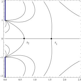
($a$)   ($b$)

Figure 1: The steepest paths when $\theta=0$: (a) when $q\in(1,\infty)$ and (b) when $q\in(0,1)$. The heavy dots indicate the saddle points and the heavy lines denote the branch cuts.

Table 1: The coefficients $c_{k}(q)$ for $0\leq k\leq 10$.

$k$	$c_{k}(q)$
0	$1$
1	$2q$
2	$6q^{2}-\leavevmode\hbox{${\textstyle\frac{1}{2}}$}$
3	$20q^{3}-4q$
4	$70q^{4}-\leavevmode\hbox{${\textstyle\frac{45}{2}}$}q^{2}+\leavevmode\hbox{${\textstyle\frac{3}{8}}$}$
5	$252q^{5}-112q^{3}+\leavevmode\hbox{${\textstyle\frac{23}{4}}$}q$
6	$924q^{6}-525q^{4}+\leavevmode\hbox{${\textstyle\frac{301}{6}}$}q^{2}-\leavevmode\hbox{${\textstyle\frac{5}{16}}$}$
7	$3432q^{7}-2376q^{5}+345q^{3}-\leavevmode\hbox{${\textstyle\frac{22}{3}}$}q$
8	$12870q^{8}-\leavevmode\hbox{${\textstyle\frac{21021}{2}}$}q^{6}+\leavevmode\hbox{${\textstyle\frac{16665}{8}}$}q^{4}-\leavevmode\hbox{${\textstyle\frac{1425}{16}}$}q^{2}+\leavevmode\hbox{${\textstyle\frac{35}{128}}$}$
9	$48620q^{9}-45760q^{7}+\leavevmode\hbox{${\textstyle\frac{139139}{12}}$}q^{5}-\leavevmode\hbox{${\textstyle\frac{1595}{2}}$}q^{3}+\leavevmode\hbox{${\textstyle\frac{563}{64}}$}q$
10	$184756q^{10}-196911q^{8}+61061q^{6}-\leavevmode\hbox{${\textstyle\frac{287287}{48}}$}q^{4}+\leavevmode\hbox{${\textstyle\frac{133529}{960}}$}q^{2}-\leavevmode\hbox{${\textstyle\frac{63}{256}}$}$

Then in case (i) we find

$$\int_{0}^{\pm i}e^{-zu}(1+u^{2})^{\nu-\frac{1}{2}}du=\int_{0}^{\infty}e^{-z\tau}\,\biggl{(}\frac{1}{\sqrt{1+u^{2}}}\,\frac{du}{d\tau}\biggr{)}d\tau\sim\sum_{k=0}^{\infty}\frac{c_{k}(q)\Gamma(k+1)}{z^{k+1}}$$

for $z\rightarrow+\infty$. Hence, for large real $\nu$ and $z$ with $\nu/z\in[1,\infty)$ (when the deformed path $C$ terminates at the branch points $u=\pm i$), we have from (1.2)

$${\bf H}_{\nu}(z)\pm iJ_{\nu}(z)\sim\frac{(\leavevmode\hbox{${\textstyle\frac{1}{2}}$}z)^{\nu-1}}{\sqrt{\pi}\Gamma(\nu+\leavevmode\hbox{${\textstyle\frac{1}{2}}$})}\,\sum_{k=0}^{\infty}\frac{c_{k}(q)\Gamma(k+1)}{z^{k}}~{},$$ (2.2)

respectively. Similarly, for $\nu/z\in(0,1)$ (when the path $C$ passes to $+\infty$ along the real axis), we have from (1.3)

$${\bf H}_{\nu}(z)-Y_{\nu}(z)\sim\frac{(\leavevmode\hbox{${\textstyle\frac{1}{2}}$}z)^{\nu-1}}{\sqrt{\pi}\Gamma(\nu+\leavevmode\hbox{${\textstyle\frac{1}{2}}$})}\,\sum_{k=0}^{\infty}\frac{c_{k}(q)\Gamma(k+1)}{z^{k}}~{}.$$ (2.3)

These are the results given in [4, §10.43]; see also the discussion in Section 3.

When $\nu$ is allowed to take on complex values with $z>0$, the steepest descent paths in Fig. 1 undergo a progressive change. Recalling that $q=\alpha+i\beta$, we find that as $\beta$ increases from zero when $\alpha\in(0,1)$ the steepest descent path from the origin $\Im\tau=0$ becomes increasingly deformed in the upper-half plane, until at a critical value $\beta=\beta^{*}$ this path connects with the saddle $S_{1}$. For example, when $\alpha=0.80$ the critical value is $\beta^{*}\doteq 0.143900$. Then, the path $\Im\tau=0$ passes to infinity when $\beta<\beta^{*}$, connects with $S_{1}$ when $\beta=\beta^{*}$ and approaches the branch point at $u=i$ (possibly spiralling onto different Riemann sheets) when $\beta>\beta^{*}$. An analogous transition occurs when $\beta<0$ at $\beta=-\beta^{*}$, with the saddle $S_{1}$ replaced by $S_{2}$. When $\alpha>1$, the steepest path $\Im\tau=0$ passes to $u=i$ when $\beta>0$, and to $u=-i$ when $\beta<0$, without undergoing any transition as $\beta$ increases.

The transitions that occur when $z>0$ and $|\arg\,\nu|\leq\leavevmode\hbox{${\textstyle\frac{1}{2}}$}\pi$ are summarised in Fig. 2(a). This shows the three curves in the complex $q$-plane, on which a transition takes place, that emanate from the point $P$ (corresponding to $q=1$). The curves in the upper and lower half-planes are conjugate curves with the third being the segment $[1,\infty)$ of the real $q$-axis. In the domain numbered 1 (between the conjugate curves and the imaginary $q$-axis), the path $C$ passes to $\infty$ and the expansion (2.3) applies. In the domain numbered 2, the path $C$ terminates at $u=+i$ and the expansion (2.2) applies with the upper sign; in the domain numbered 3, the terminal point is $u=-i$ and the expansion (2.2) applies with the lower sign. For $q$ situated on these curves the transition is associated with a Stokes phenomenon; see below.

3.  Asymptotic expansion for complex $z$

When $z$ is complex ($\theta\neq 0$) the transition curves in the sector of the $q$-plane given by $(-\leavevmode\hbox{${\textstyle\frac{1}{2}}$}\pi-\theta,\leavevmode\hbox{${\textstyle\frac{1}{2}}$}\pi-\theta)$ are $\theta$-dependent. In Fig.2(b)–(d) we show these curves for $\theta/\pi=0.10$, $0.20$ and $0.30$. The curves for $\theta<0$ are the conjugate of those for $\theta>0$. The point $P$ corresponds to the case when the steepest descent path from the origin connects with both saddles $S_{1}$ and $S_{2}$. The point labelled $Q$ is the intercept of the lower curve with the positive $q$-axis. Values of $q$ at $P$ and $Q$ are presented in Table 2 for different $\theta$.

Table 2: The coordinates of the triple point $P$ and the intercept $Q$ on the real $q$-axis as a function of $\theta$.

$\theta/\pi$	$P$	$Q$	$\theta/\pi$	$P$	$Q$
0	$1$	$1$	0.30	$1.08553+1.38238i$	$0.27561$
0.05	$0.96385+0.08606i$	$0.83360$	0.35	$1.36479+2.60425i$	$0.18575$
0.10	$0.93778+0.18745i$	$0.70952$	0.40	$2.36238+7.23955i$	$0.10710$
0.20	$0.93437+0.53249i$	$0.48057$	0.42	$3.72266+14.4826i$	$0.07942$
0.25	$0.97678+0.84047i$	$0.37449$	0.45	$16.4886+104.102i$	$0.04275$

As in the case $\theta=0$ in Fig. 2(a), for $q$-values in domain 1 the endpoint of the steepest descent path from the origin terminates at infinity, whereas those situated in domains 2 and 3 pass to the branch points (possibly spiralling onto adjacent Riemann surfaces) at $u=\pm i$, respectively. As one crosses one of these curves, say from domain 1 to domain 2, there is a change in the endpoint via a Stokes phenomenon. Examples of the steepest descent paths when $\theta=0.10\pi$ on the three curves labelled $PA$, $PB$ and $PC$ in Fig. 2(b), and at $P$, are shown in Fig. 3 demonstrating that on each curve the change of endpoint is associated with a Stokes phenomenon.

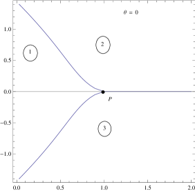
($a$)   ($b$)

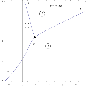
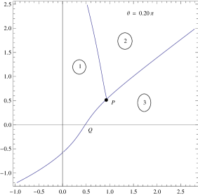
($c$)  ($d$)

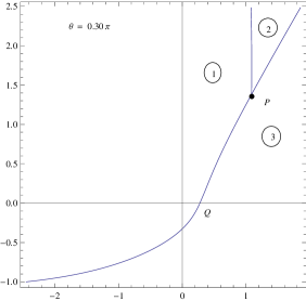
Figure 2: The domains in the sector of the $q$-plane bounded by $-\leavevmode\hbox{${\textstyle\frac{1}{2}}$}\pi-\theta<\omega<\leavevmode\hbox{${\textstyle\frac{1}{2}}$}\pi-\theta$ showing the termination points of the steepest descent path from the origin: (a) $\theta=0$, (b) $\theta=0.10\pi$, (c) $\theta=0.20\pi$ and (d) $\theta=0.30\pi$. The termination point in domain 1 is at infinity and that in domains 2 and 3 is at $\pm i$, respectively.

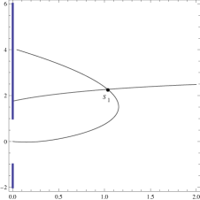
($a$)   ($b$)

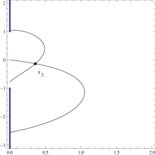
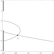
($c$)  ($d$)

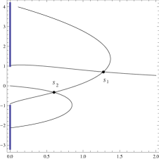
Figure 3: The steepest paths the through the saddles when $\theta=0.10\pi$: (a) on $PA$ with $q=0.60+0.95307i$, (b) on $PB$ with $q=1.40+0.39447i$, (c) on $PC$ with $q=0.40-0.42914i$ and (d) at $P$ with $q=0.93778+0.18745i$. The heavy lines denote the branch cuts.

4.  Numerical results

To verify these assertions, we carry out calculations using (2.2) and (2.3) for a series of values of $q\equiv\nu/z$ situated in different domains in Fig. 2. The results are presented in Table 3 which shows the absolute relative error in the computation of ${\bf H}_{\nu}(z)$. The values of the Bessel functions $J_{\nu}(z)$ and $Y_{\nu}(z)$ were evaluated with the in-built codes in Mathematica. In each case, the asymptotic series on the right-hand sides of (2.2) and (2.3) is optimally truncated; that is, at or just before the least term.

Table 3: The absolute relative error in the computation of ${\bf H}_{\nu}(z)$ from (2.2) and (2.3) when $z=40e^{i\theta}$.

	$\theta=0$		$\theta=0.10\pi$
$q=\nu/z$	Error	Endpoint	Error	Endpoint
$0.60$	$7.764\times 10^{-9}$	$\infty$	$9.556\times 10^{-9}$	$\infty$
$1.00$	$1.041\times 10^{-4}$	$\pm i$	$2.751\times 10^{-5}$	$-i$
$1.25$	$8.835\times 10^{-4}$	$\pm i$	$4.830\times 10^{-4}$	$-i$
$0.60+0.40i$	$2.355\times 10^{-6}$	$\infty$	$3.280\times 10^{-6}$	$\infty$
$1.00+0.60i$	$2.783\times 10^{-4}$	$+i$	$4.136\times 10^{-3}$	$+i$
$1.00-0.30i$	$7.342\times 10^{-5}$	$-i$	$5.000\times 10^{-5}$	$-i$

In [4, §10.43], Watson claims that (2.3) and (2.2) hold for $q\in(0,1)$ and $q\in[1,\infty)$, respectively, when $|\arg\,z|<\leavevmode\hbox{${\textstyle\frac{1}{2}}$}\pi$. Our calculations have shown that when $\arg\,z\neq 0$ with $q=\nu/z>0$ (that is, when $\nu$ and $z$ have the same phase), the expansion (2.3) holds for $q\in(0,Q)$ and the expansion (2.2) holds for $q\in[Q,\infty)$, where $Q\equiv Q(\theta)$ is tabulated in Table 2.