Overlapping group logistic regression with applications to genetic pathway selection

Abstract

Discovering important genes that account for the phenotype of interest has long been challenging in genomewide expression analysis. Analyses such as Gene Set Enrichment Analysis (GSEA) that incorporate pathway information have become widespread in hypothesis testing, but pathway-based approaches have been largely absent from regression methods due to the challenges of dealing with overlapping pathways and the resulting lack of available software. The R package grpreg is widely used to fit group lasso and other group-penalized regression models; in this study, we develop an extension, grpregOverlap, to allow for overlapping group structure using the latent variable approach proposed by Jacob et al. (2009). We compare this approach to the ordinary lasso and to GSEA using both simulated and real data. We find that incorporation of prior pathway information substantially improves the accuracy of gene expression classifiers, and we shed light on several ways in which hypothesis-testing approaches such as GSEA differ from regression approaches with respect to the analysis of pathway data.

Keywords: Overlapping group lasso; Penalized logistic regression; Gene set enrichment analysis; Pathway selection.

1 Introduction

Since the original proposal of the lasso by Tibshirani (1996), penalized regression methods for variable selection in high-dimensional settings have attracted considerable attention in modern statistical research. These methods have been extensively studied in theory and widely applied in practice. Most of the methods focus on selecting individual explanatory variables (or predictors). In many settings, however, predictors possess a group structure. Incorporating this grouping information into the modeling process has the potential to improve both the interpretability and accuracy of the model.

Consider first the linear regression problem with $J$ non-overlapping groups,

$$\mathbf{y}=\sum_{j=1}^{J}\mathbf{X}^{j}\bm{\beta}^{j}+\bm{\epsilon}$$ (1)

where $\mathbf{y}$ is an $n\times 1$ response vector, $\bm{\epsilon}\sim N_{n}(\mathbf{0},\sigma^{2}\mathbf{I})$, $\mathbf{X}^{j}$ is an $n\times K^{j}$ matrix corresponding to the $j$th group, $K^{j}$ is the number of elements in group $j$, and $\bm{\beta}^{j}$ is the associated $K^{j}\times 1$ coefficient vector. In (1), we take $\mathbf{y}$ to be centered, thereby eliminating the need for an intercept. To perform variable selection at the group level, Yuan and Lin (2006) proposed the group lasso estimator, defined as the value $\bm{\beta}$ minimizing

$$Q(\bm{\beta})=L(\bm{\beta}\mid\mathbf{y},\mathbf{X})+\lambda\sum_{j=1}^{J}\sqrt{K^{j}}\|\bm{\beta}^{j}\|$$ (2)

where $\|\cdot\|$ is the Euclidean ($l_{2}$) norm and $L(\bm{\beta}\mid\mathbf{y},\mathbf{X})$ is the loss function. For linear regression, the loss function is simply the residual sum of squares, i.e., $\|\mathbf{y}-\mathbf{X}\bm{\beta}\|^{2}/2n$. For other models, it can be any term that quantifies the fit of the model; for example, Meier et al. (2008) extended the group lasso selection to logistic regression by using the negative log-likelihood as the loss function. The second term in (2) is called the group lasso penalty or $l_{1}/l_{2}$ penalty since it is the weighted sum of the $l_{2}$ norms of the group coefficient vectors. The group lasso penalty leads to variable selection at the group level. That is, the coefficient estimates of the variables in the $j$th group will be all non-zero if group $j$ is selected and all zero otherwise.

An obvious limitation of the group lasso, however, is that it assumes that the groups do not overlap. This introduces a barrier to its application for many problems where variables may be included in more than one group. For instance, in the analysis of gene expression profiles, individual genes can be grouped into pathways, in which the collective action of several genes is required in order for the cell to carry out a complicated function. These pathways generally overlap with each other as one gene can play a role in multiple pathways.

In recent years, various pathway-based approaches have been proposed for analyzing gene expression data (Nam and Kim, 2008). One key assumption of these methods is that weak expression changes in individual genes are coordinated and can be combined in groups to produce stronger signals. Hence, by incorporating prior pathway information, these approaches aim to identify differentially expressed pathways, instead of individual genes. Compared to traditional single-gene tests, pathway-based tests often lead to higher statistical power and better biological interpretation. Among the pathway-testing approaches, Gene Set Enrichment Analysis (GSEA, Mootha et al., 2003; Subramanian et al., 2005) has been widely used. The hypothesis testing framework has certain limitations for pathway analysis, however, such as the inability to account for the effect of multiple genes simultaneously, and it is not well-suited to using gene expression and pathway data to predict biological outcomes (Goeman and Bühlmann, 2007).

On the other hand, pathway-based approaches have been largely absent from regression methods due to the challenges of dealing with overlapping pathways in regression models. To address this issue, Jacob et al. (2009) proposed a latent group lasso approach for variable selection with overlapping groups, making it possible to perform pathway selection under the general linear modeling framework.

In this paper, we formulate the overlapping group logistic regression model for pathway selection, and compare this overlapping group lasso (OGLasso) approach to both the ordinary lasso and GSEA via both simulation and real data studies. The paper is organized as follows. In Section 2, we review the overlapping group lasso approach, and construct the overlapping group lasso model. In addition, we give a brief introduction to GSEA, along with some discussions. In Section 3, we first compare the ordinary lasso and OGLasso in terms of model accuracy with simulated data. Then we examine the group selection accuracy of OGLasso and GSEA under different simulation settings. In addition, we provide two real data studies in Section 4. We conclude the paper with final discussions in Section 5.

In addition, we have provided a publicly available implementation of the overlapping group lasso method described in this article through the R package grpregOverlap. This package serves as an extension of the R package grpreg, which provides a variety of functions for fitting penalized regression models involving grouped predictors, but requires those groups to be non-overlapping.

2 Methods

2.1 Overlapping group lasso

Suppose the $p$ predictors $\{x_{1},x_{2},\ldots,x_{p}\}$ are assigned into $J$ possibly overlapping groups (i.e., a given predictor $x_{i}$ may be included in more than one group). The group lasso estimator (2) does not necessarily select groups in this overlapping setting. For example, suppose $p=3$ and $J=2$, with one covariate shared between the two groups: group “A” and group “B”, with group A truly related to the outcome. If group B is not selected, then all of its coefficients are zero, even though one coefficient also appears in group A. Thus, group A is only partially selected. This problem is greatly exacerbated as the groups grow in size and complexity, and is described in greater detail in Jenatton et al. (2011).

To select entire groups of covariates in the overlapping setting, Jacob et al. (2009) proposed the overlapping group lasso, formulated as

$$\begin{split}\min_{\bm{\beta}}\;Q(\bm{\beta})&=L(\bm{\beta}\mid\mathbf{y},\mathbf{X})+\lambda\sum_{j=1}^{J}\sqrt{K^{j}}\|\bm{\gamma}^{j}\|\\ \textrm{subject to }\bm{\beta}&=\sum_{j=1}^{J}\bm{\gamma}^{j},\end{split}$$ (3)

where $\{\bm{\gamma}^{j}\}^{J}_{j=1}$ are $J$ so-called latent coefficient vectors. The collection of latent vectors $\bm{\gamma}^{j}=(\gamma_{1}^{j},\gamma_{2}^{j},\ldots,\gamma_{p}^{j})^{\prime}$ satisfies $\sum_{j=1}^{J}\bm{\gamma}^{j}=\bm{\beta}$, and $\gamma_{k}^{j}=0$ if $x_{k}$ does not belong to group $j$, with $\gamma_{k}^{j}\neq 0$ otherwise.

The idea of model (3) is to decompose the original coefficient vector into a sum of group-specific latent effects. This decomposition allows us to apply the group lasso penalty to the latent vectors $\{\bm{\gamma}^{j}\}^{J}_{j=1}$, which do not overlap, instead of the original, overlapping coefficients. Consequently, when a latent vector $\bm{\gamma}^{j}$ is selected, all covariates in group $j$ will be selected, even if some members of the group are also involved in unselected groups.

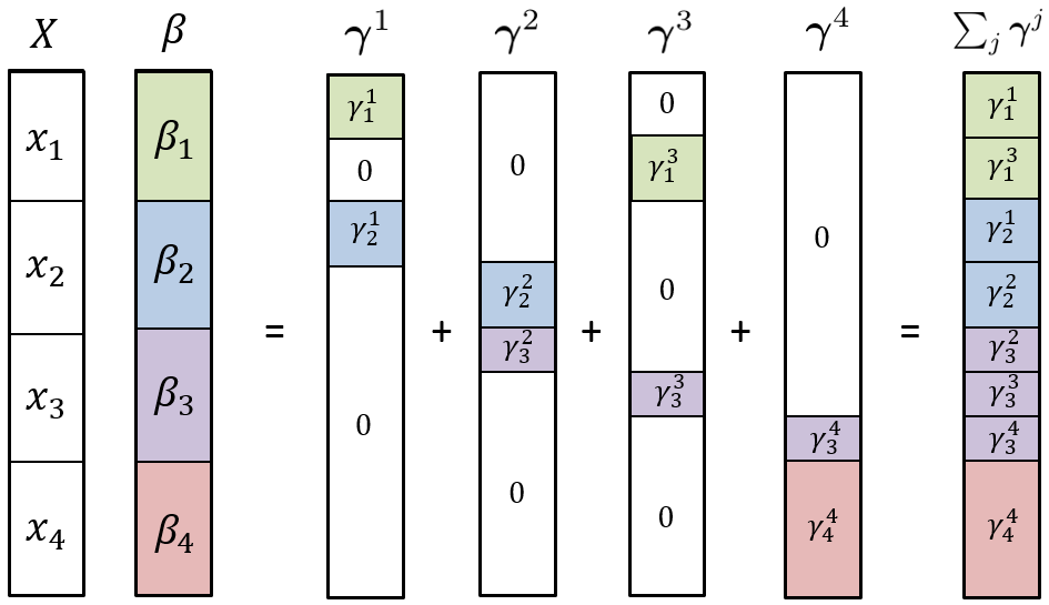
Figure 1: The coefficient decomposition of overlapping group lasso.

Figure 1 illustrates the coefficient decomposition mechanism stated above. Suppose that there are 4 variables $x_{1},x_{2},x_{3},x_{4}$ that are included in four groups, $S^{1}=\{x_{1},x_{2}\},\,S^{2}=\{x_{2},x_{3}\},\,S^{3}=\{x_{1},x_{3}\},\,S^{4}=\{x_{3},x_{4}\}$, where $S^{j}$ denote the set of variables in group $j$. Since $x_{1}$ is in both group 1 and 3, $\beta_{1}$ is thus decomposed into $\gamma_{1}^{1}+\gamma_{1}^{3}$. Likewise, $\beta_{3}$ is decomposed into $\gamma_{3}^{2}+\gamma_{3}^{3}+\gamma_{3}^{4}$, and so on. Suppose group 1 is the sole truly nonzero group in this example. The overlapping group lasso model can select $\bm{\gamma}^{1}$, thereby indirectly selecting $\beta_{1}$ and $\beta_{2}$ and eliminating $\beta_{3}$ and $\beta_{4}$ since they do not appear in group 1. Note that the original group lasso cannot accomplish this – if group 3 is eliminated, then predictor 1 is eliminated as well since it belongs to group 3.

Based on the coefficient decomposition, model (3) can be transformed into a new minimization problem (Obozinski et al., 2011) with respect to $\bm{\gamma}$:

$$\min_{\bm{\gamma}}\;Q(\bm{\gamma})=L(\bm{\gamma}\mid\mathbf{y},\,\widetilde{\mathbf{X}})+\lambda\sum_{j=1}^{J}\sqrt{K^{j}}\|\bm{\gamma}^{j}\|.$$ (4)

Here, $\bm{\gamma}$ in principle consists of all elements of $\bm{\gamma}^{j}$, although in practice one can leave off the zero elements as they have no effect on the objective function. The new design matrix $\widetilde{\mathbf{X}}$ is constructed by duplicating the columns of overlapped variables in the raw design matrix $\mathbf{X}$, where appropriate, to match the elements of $\bm{\gamma}$. The equivalence of the loss functions $L(\bm{\beta}\mid\mathbf{y},\mathbf{X})$ and $L(\bm{\gamma}\mid\mathbf{y},\,\widetilde{\mathbf{X}})$ can be seen by observing that $\mathbf{X}\bm{\beta}=\mathbf{X}\sum_{j}\bm{\gamma}^{j}=\widetilde{\mathbf{X}}\bm{\gamma}$.

The implication of (4) is that the overlapping group lasso problem is equivalent to a classical group lasso in an expanded, non-overlapping space. This is of considerable practical convenience, as it allows us to solve (4) using computationally efficient algorithms that have previously been developed for the group lasso (Breheny and Huang, 2015).

2.2 Overlapping group logistic regression

It is relatively straightforward to extend (4) to models other than linear regression; in this section, we describe its application to penalized logistic regression in the presence of overlapping groups. Here, $\mathbf{y}$ is the response vector of binary entries, and the intercept $\beta_{0}$ cannot be removed by centering $\mathbf{y}$. For convenience, we assume the first column of the design matrix $\mathbf{X}$ is the unpenalized column of 1’s for the intercept $\beta_{0}$, and denote $\mathbf{x}_{i}=(1,x_{i1},\ldots,x_{ip})^{\prime}$ for $i=1,\ldots,n$. Correspondingly, we denote $\bm{\beta}=(\beta_{0},\beta_{1},\ldots,\beta_{p})^{\prime}$. The logistic regression model is

$$\textrm{Pr}(y_{i}=1\mid\mathbf{x}_{i})=\pi_{i}=\frac{\exp(\mathbf{x}_{i}^{\prime}\bm{\beta})}{1+\exp(\mathbf{x}_{i}^{\prime}\bm{\beta})}.$$ (5)

The corresponding loss function is the (scaled) negative log-likelihood function,

$$L(\bm{\beta}\mid\mathbf{y},\mathbf{X})=-\frac{1}{n}\sum_{i=1}^{n}\{y_{i}(\mathbf{x}_{i}^{\prime}\bm{\beta})-\log(1+\exp(\mathbf{x}_{i}^{\prime}\bm{\beta}))\}.$$

We can then duplicate the columns of the overlapped covariates, expanding the design matrix to $\widetilde{\mathbf{X}}$ as described previously, and construct the overlapping group logistic regression model in the same fashion as model (4), with

$$L(\bm{\gamma}\mid\mathbf{y},\,\widetilde{\mathbf{X}})=-\frac{1}{n}\sum_{i=1}^{n}\{y_{i}(\widetilde{\mathbf{x}}_{i}^{\prime}\bm{\gamma})-\log(1+\exp(\widetilde{\mathbf{x}}_{i}^{\prime}\bm{\gamma}))\}$$ (6)

where $\widetilde{x_{i}}^{\prime}$ is the $i$th row of the expanded design matrix $\widetilde{\mathbf{X}}$, and the first element of $\bm{\gamma}$ is the unpenalized intercept $\beta_{0}$.

2.3 Gene set enrichment analysis (GSEA)

Among the hypothesis-testing approaches for pathway selection, GSEA stands out due to its relative simplicity and for preserving the gene-gene dependencies that occur in real biological data (Tamayo et al., 2012).

The procedure of GSEA (Subramanian et al., 2005) starts with ranking the $p$ genes by the correlation, $r_{j}$, between each gene and the phenotype. Then a test statistic, the enrichment score (ES), is calculated for each gene set by walking down the ranked gene list and accumulating the correlation information: increasing ES by $|r_{i}|^{\alpha}/\sum_{j\in S}|r_{j}|^{\alpha}$ if gene $i$ is included in gene set $S$; decreasing ES by $1/(p-|S|)$ otherwise. Here $\alpha$ is a pre-specified exponent parameter. When $\alpha=1$, ES corresponds to the normalized Kolmogorov-Smirnov statistic. Next, the significance level of the ES is assessed by a permutation test. Finally, the significance of the gene sets is determined by controlling the false discovery rate (FDR).

Though widely used, GSEA also has several limitations. First, GSEA may be biased in favor of larger gene sets by systematically assigning those gene sets higher ES (Damian and Gorfine, 2004); Second, it implicitly assumes genes within the same gene set show coordinated (i.e., either all positive or all negative) associations with the phenotype, making it less likely to detect sets in which the genes are heterogeneous with respect to the direction of association with the phenotype (Dinu et al., 2007).

There are inherent differences between GSEA and the proposed overlapping group logistic regression method in the sense that GSEA treats the phenotype as fixed and gene expression as random, while regression-based methods do the opposite. Thus, GSEA tends to be more appropriate in settings where the phenotype can be directly manipulated by the experiment (e.g., knockout mice), while regression is more appropriate in observational settings (e.g., predicting patient outcomes). Nevertheless, there are many situations in which either method could reasonably be used, and therefore, it is of interest to compare the selection properties of the two approaches.

3 Simulation studies

In all of the simulation studies, we use the term “null group” to denote a group whose coefficients are all equal to zero in the true model, and “true group” to denote a group with all non-zero coefficients in the true model. In addition, we refer to $\|\bm{\gamma}^{j}\|$ as the effect of group $j$, and $\gamma_{k}^{j}$ as the latent effect of covariate $k$ in group $j$.

3.1 Overlapping group lasso vs. ordinary lasso

We start by comparing the overlapping group lasso (OGLasso) with the ordinary lasso in terms of estimation and prediction accuracy. We use root mean squared error (RMSE) to measure estimation accuracy and misclassification error (ME) to measure prediction accuracy, defined as follows:

$$\text{RMSE}=\sqrt{\frac{1}{p}\sum_{k=1}^{p}(\beta_{k}-\hat{\beta}_{k})^{2}}~{};\quad\text{ME}=\frac{\text{\# incorrectly classified}}{\text{Sample size}}$$

It should be noted that we compute ME based on a new response vector generated by the same design matrix for each replication. Specifically, given a design matrix $\mathbf{X}$, two response vectors $\mathbf{y}$ and $\mathbf{y}^{*}$ are simulated. The data $\{\mathbf{X},\mathbf{y}\}$ is used to fit the model, and its prediction accuracy is tested on data $\{\mathbf{X},\mathbf{y}^{*}\}$.

We consider two simulations with different settings described as follows.

Setting 1: Synthetic data. We begin with synthetic data where there are 15 groups of covariates. All covariate values are simulated independently from a standard Gaussian distribution. The group sizes and overlap structure are presented below.

ID: $1\quad 2$ $3$ $4\quad 5$ $6$ $7\quad 8$ $9$ $10\quad 11$ $12$ $13\quad 14$ $15$ Size: $\underbrace{10\quad 10}_{3}$ $10$ $\underbrace{10\quad 10}_{3}$ $10$ $\underbrace{10\quad 10}_{3}$ $10$ $\underbrace{10\quad 10}_{3}$ $10$ $\underbrace{10\quad 10}_{3}$ $10$

The number underneath the brace is the number of members shared between those two groups. For example, group 1 contains 10 members, as does group 2, but the two groups contain only 17 unique predictors, as 3 predictors are present in both groups. As a result, the total dimension in this setting is $p=135$. By design, groups 1, 4, 7, 10, and 13 are set to be true groups. The sample size is set to be $n=50$ to be consistent with that in Setting 2 as below.

Setting 2: Real data. For this simulation, a real gene expression profile data set in the p53 study (Subramanian et al., 2005) is used as the design matrix to mimic the complicated correlation and overlapping structures in real biomedical applications. This design matrix is fixed for each independent replication. Here, the sample size $n=50$, the number of genes $p=4301$, and the number of pathways (groups) is 308; a more detailed description of the study is given in Section 4. We chose 5 pathways, with sizes 15, 16, 20, 26, and 40, to represent the true groups in this simulation. The number of overlaps between the 5 pathways ranges from 0 to 9.

In both of the two above settings, the true group effect of each of the 5 true groups is set to be equal, and the latent effects are also set to be equal within each true group. In this way, the true coefficient vector is uniquely specified. Then given the design matrix, the responses are generated according to (5) for each independent replication. The true group effect is varied from 1 to 5 to simulate different magnitudes of signals.

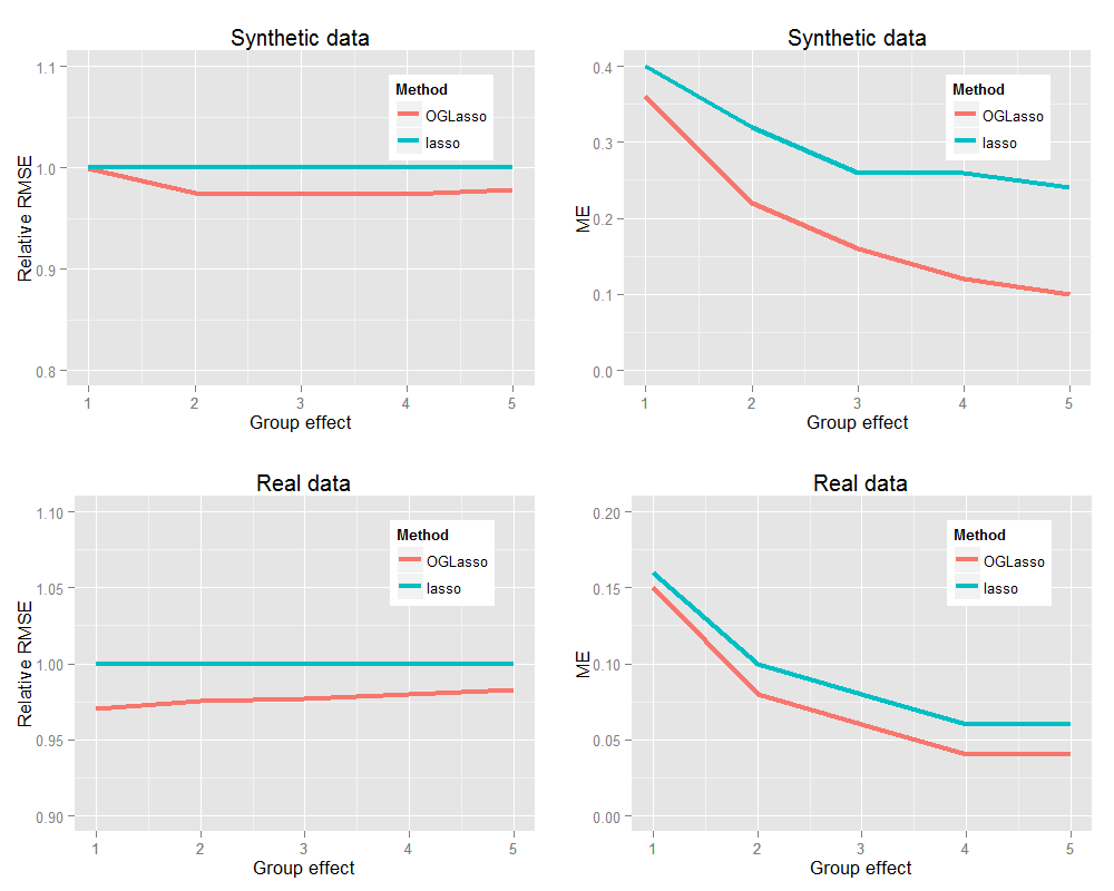
Figure 2: Accuracy of OGLasso and ordinary lasso with respect to the magnitude of the group effect. Top two panels summarize results for the Synthetic data simulation, while bottom two panels are for the Real data simulation. Left panels: Median RMSE relative to ordinary lasso over 500 replications. Right panels: Median ME over 500 replications.

Figure 2 illustrates the estimation and prediction accuracy of the proposed grouped variable selection method, as compared to the ordinary lasso, for both settings. The top two panels show results for the synthetic data simulation, while the bottom two panels are for the real data simulation. The left panels illustrate the median RMSE relative to ordinary lasso over 500 replications, while the right panels compare the methods in terms of ME. OGLasso consistently achieves a lower median RMSE than that of the lasso in both synthetic and real data simulations. As expected, the misclassification error by both methods decreases as the coefficient magnitude increases. More interestingly, the misclassification error by OGLasso can be substantially lower than that of ordinary lasso. In the synthetic data simulation, for example, the misclassification error by OGLasso is more than 10% lower than that of ordinary lasso when the group effect is 4. The two methods are more similar in terms of predictive accuracy on the real data, where the dimensionality is much higher and correlation structure more complicated. Nevertheless, the prediction accuracy can still be improved by around 2% with OGLassso compared to ordinary lasso.

3.2 Overlapping group lasso vs. GSEA

In this section, we use simulated data to compare the selection properties of the overlapping group lasso against GSEA in a variety of different settings. Because OGLasso and GSEA do not estimate the same quantities and GSEA does not produce predictions, the only way to compare them is with respect to selection accuracy. To ensure a fair comparison, we use each method to select a fixed number of groups. We then evaluate the group selection accuracy by the true discovery rate (TDR):

$$\text{TDR}=\frac{\text{\# of true groups selected}}{\text{\# of groups selected}},$$

where the # of groups selected was fixed at 5 (i.e., each method was used to identify the five most important-looking groups). In each of the following simulations, the results are based on sample size $n=100$ and averaged over 500 independent replications.

Setting 3: Unequal group size. First, we investigate the performance of the two approaches when group sizes are unequal. In this simulation, the design matrix consists of 15 groups with all covariate values simulated independently from a standard Gaussian distribution. The group sizes and overlap structure are shown below.

ID: $1\quad 2$ $3$ $4\quad 5$ $6$ $7\quad 8$ $9$ $10\quad 11$ $12$ $13\quad 14$ $15$ Size: $\underbrace{3\quad 3}_{1}$ $3$ $\underbrace{6\quad 6}_{2}$ $6$ $\underbrace{9\quad 9}_{3}$ $9$ $\underbrace{15\quad 15}_{5}$ $15$ $\underbrace{24\quad 24}_{8}$ $24$

The overlap here is designed to be 1/3 of the size of overlapped groups. As a result, the total dimension in this setting is $p=152$. Moreover, groups 1, 4, 7, 10, and 13 are set to be true groups with $\|\bm{\gamma}^{j}\|=5$, and the others are null groups with $\bm{\gamma}^{j}=\mathbf{0}$. The latent effects are again set to be equal within each true group.

Table 1: The mean (standard error) of TDR and average size of selected groups of OGLasso and GSEA over 500 replications.

Method TDR Average size OGLasso 0.77 (0.01) 8.8 (0.1) GSEA 0.79 (0.01) 11.0 (0.1)

Table 1 summarizes the mean TDR and size of selected groups for the overlapping group Lasso and GSEA over 500 replications. The two methods are comparable in terms of TDR, while the average size of selected groups from GSEA is slightly larger.

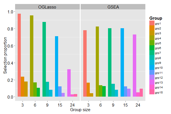
Figure 3: Comparison of the proportion of each group being selected over 500 replications.

The proportion of each group selected is depicted in Figure 3. OGLasso tends to favor groups with smaller size, while GSEA has roughly an equal probability of selecting a true group regardless of its size. This is understandable, as regression-based methods have a built-in mechanism for encouraging parsimony, unlike GSEA. Whether this preference for smaller groups is desirable or not depends on the application and the scientific goals of the study.

Setting 4: Heterogeneous gene effects. Previous studies have shown that GSEA is less likely to detect sets of genes containing both positive and negative associations with the phenotype (Dinu et al., 2007). This is because, by pooling together correlations, GSEA assumes that the genes in a set have a coordinated effect – i.e., that they all act in the same direction. In this simulation, we examine this aspect of GSEA further and demonstrate that the exhibition of heterogeneous effects among genes in a set deteriorates the statistical power of GSEA.

We employ the same configuration as in Setting 1 of Section 3.1 for the design matrix (except that the sample size here is $n=100$), but specify the true coefficient values in a different manner. Specifically, we draw the true latent coefficients $\gamma_{k}^{j}$ for each true group from a Unif($\mu-\sigma,\mu+\sigma$) distribution. Here $\sigma$ is a parameter that controls the degree of heterogeneity (or variability) of the gene effects. The larger $\sigma$ is, the more heterogeneous the effects are. In this simulation, we vary $\sigma$ to examine the effect of heterogeneity on the TDR of each method.

On a technical note, it must be pointed out that varying $\sigma$ will also change the group effect, $\|\bm{\gamma}^{j}\|$. To suppress this possibly confounding effect, we adjust $\mu$ along with $\sigma$ so that the (root-mean-square) group effect remains constant. Specifically, choosing $\mu=\sqrt{\frac{5}{2}-\frac{1}{3}\sigma^{2}}$ results in a constant $\sqrt{\mathbb{E}(\|\bm{\gamma}^{j}\|^{2})}=5$ for all values of $\sigma$.

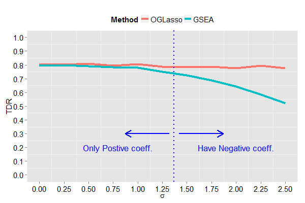
Figure 4: Comparison of OGLasso and GSEA in terms of TDR as a function of heterogeneity parameter $\sigma$. The blue dotted line indicates $\sigma=1.37$, after which negative coefficients can occur by design. The mean values over 500 replications are displayed.

Figure 4 compares OGLasso and GSEA in terms of TDR as a function of $\sigma$. OGLasso is essentially unaffected by heterogeneity: it detects approximately 4 out of the 5 true groups regardless of the magnitude of heterogeneity. In contrast, the TDR of GSEA decreases as $\sigma$ increases. This effect is apparent even when all genes in a group have a consistent direction, although the effect is much more significant for $\sigma>1.37$, at which point it is possible for genes within a true group to have opposite directions.

Setting 5: Correlation among genes. In this simulation, we assess how correlation among genes affects group selection. We use the same settings for the groups and overlap structure as in Setting 1, where $p=135$. The true coefficients are fixed so that the group effect $\|\bm{\gamma}^{j}\|=5$ for each true group, and that all latent effects $\gamma_{k}^{j}$ within a true group $j$ are equal. In this setting, covariates are no longer independent, but are instead simulated from a multivariate Gaussian distribution with mean $\mathbf{0}$ and variance $\bm{\Sigma}$. We impose a block-diagonal covariance structure with 5 compound-symmetric blocks, as shown below:

$$\bm{\Sigma}=\begin{bmatrix}\Sigma&&&&\\ &\Sigma&&&\\ &&\Sigma&&\\ &&&\Sigma&\\ &&&&\Sigma\end{bmatrix},\text{where }\Sigma=\begin{bmatrix}1&\rho&\cdots&\rho\\ \rho&1&\cdots&\rho\\ \vdots&\vdots&\ddots&\vdots\\ \rho&\rho&\cdots&1\\ \end{bmatrix}_{27\times 27}$$

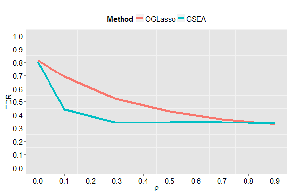
Figure 5: Comparison of OGLasso and GSEA in terms of TDR as a function of pairwise correlation $\rho$. The mean values over 500 replications are displayed.

Figure 5 compares OGLasso and GSEA in terms of TDR as a function of pairwise correlation $\rho$. As expected, TDR of both methods decreases as the correlation among genes increases. However, GSEA is much more strongly affected by correlation than the overlapping group lasso. For example, as $\rho$ increases from 0 to 0.1, the TDR of GSEA drops from around 0.8 to 0.45. This ability – to adjust for correlation between pathways – is one of the primary potential advantages of a regression-based approach over a hypothesis-testing approach, which is limited to considering a single pathway at a time.

4 Real data studies

In this section, we analyze the data from two gene expression studies reported in Subramanian et al. (2005), one involving the mutational status of p53 in cell lines and the other involving the prognosis of lung cancer patients.

The p53 study aims to identify pathways that correlated with the mutational status of the gene p53, which regulates gene expression in response to various signals of cellular stress. The p53 data  (Olivier et al., 2002) consist of 50 cell lines, 17 of which are classified as normal and 33 of which carry mutations in the p53 gene. To be consistent with the analysis in Subramanian et al. (2005), 308 gene sets that have size between 15 and 500 are included in our analysis. These gene sets contain a total of 4301 genes.

The lung cancer data (Beer et al., 2002) contains gene expression profiles in 86 tumor samples, out of which 24 are classified as “poor” outcome and the remaining as “good” outcome. The data sets are preprocessed in the same fashion as in the p53 study, resulting in 258 gene sets that contain a total of 3256 genes. Compared to the p53 data, the lung cancer data show much weaker signals: no individual gene is found to be significant in a conventional single-gene analysis.

We first compare the OGLasso to the ordinary lasso in terms of prediction accuracy. For each method, 10-fold cross-validation was used to choose the regularization parameter $\lambda$.

Table 2: Real data studies: 10 fold cross-validated misclassification error (ME) for different models. “Baseline” is the intercept-only model.

Method p53 study lung cancer study Baseline 0.34 0.28 lasso 0.26 0.30 OGLasso 0.20 0.27

Indeed, as shown in Table 2, the incorporation of pathway information into the regression model produces more accurate predictions in both studies. In the p53 study, where the signals are relatively strong, the misclassification error of the ordinary lasso is 8% lower than that of the intercept-only model. The OGLasso, however, can further lower the error by an additional 6%. In the lung cancer study, due to a small signal-to-noise ratio, the ordinary lasso performed even worse than the intercept-only model. The OGLasso, however, was able to improve on the predictions of the intercept-only model, albeit only slightly.

We now turn to comparing the pathways selected by OGLasso and GSEA. Again, 10-fold cross-validation is used to select $\lambda$ for OGLasso, while a FDR cutoff of 0.25 was used to select pathways with GSEA. Table 3 lists the number of pathways, the number of total genes and number of unique genes in those selected pathways by OGLasso and GSEA. In both studies, GSEA selects more pathways than OGLasso, especially in the lung cancer study (21 vs. 3). Moreover, in agreement with our earlier simulation results, GSEA selects substantially larger pathways than OGlasso. For example, in the lung cancer study the average pathway size for GSEA is 820/21=39 genes, while the average size for OGLasso is only 51/3=17 genes.

Table 3: Real data studies: number of selected pathways (# Pathways), number of total genes (# Total Genes), and number of unique genes (# Unique Genes) in selected pathways by OGLasso and GSEA.

Method p53 study lung cancer study # Pathways # Total # Unique # Pathways # Total # Unique Genes Genes Genes Genes OGLasso 3 46 44 3 51 50 GSEA 6 139 105 21 820 629

Table 4 presents a summary of pathway selection results in the p53 study that sheds light on the nature of the pathways selected by each approach. Naturally, both approaches identify the “p53Pathway” as being associated with p53 mutation status. However, GSEA also selects pathways “radiation_sensitivity”, which shares 9 genes with “p53Pathway”, “p53hypoxiaPathway” (7 shared genes), and “P53_UP” (5 shared genes). From a regression perspective, these four pathways are largely redundant, and the three unselected pathways carry no additional useful information beyond that already contained in the p53 pathway. On the other hand, OGLasso selects one pathway, “ck1Pathway”, not identified by GSEA. Although the ck1 pathway has a weaker marginal relationship with p53 mutation status than the hsp27 and p53 pathways, the information it contains is largely independent of the other pathways included in the model (no overlaps with the hsp27 and p53 pathways), potentially shedding light on novel p53 relationships that would not be apparent from the GSEA approach.

Table 4: The p53 study: pathways selected by OGLasso and GSEA with FDR $\leq 0.25$.

Pathway label Size FDR $q$ value GSEA OGLasso hsp27Pathway 15 $<.001$ ✓ ✓ p53hypoxiaPathway 20 $<.001$ ✓ p53Pathway 16 $<.001$ ✓ ✓ radiation_sensitivity 26 $0.078$ ✓ P53_UP 40 $0.013$ ✓ rasPathway 22 $0.171$ ✓ ck1Pathway 15 $0.500$ ✓

The biological interpretations of the pathways selected in the lung cancer study are less clear due to the weaker signals and more complicated biological outcome. Nevertheless, there are some interesting similarities and differences here as well. Of the three gene sets selected by OGLasso, one pathway (ceramide) is also selected by GSEA. The other two gene sets, although not selected by GSEA, contain a fair amount of overlap with GSEA-selected sets. For example, OGLasso selects the Fas pathway while GSEA selects the p53 pathway. However, both pathways are involved in apoptosis, and 6 genes are shared between the two pathways. The simulation studies of Section 3.2 suggest that differences in the size, heterogeneity, or correlation patterns of these pathways provide an explanation for why OGLasso prefers the Fas pathway to the p53 pathway.

5 Discussion

Pathway-based approaches for analyzing gene expression data have become increasingly popular in recent years. Most methods have approached the problem from a multiple hypotheses testing perspective. However, the overlapping group lasso approach proposed by Jacob et al. (2009) allows the incorporation of pathway information into regression models as well.

In this paper, we present evidence that the incorporation of pathway information can substantially improve the accuracy of gene expression classifiers. Furthermore, we provide open-source software, publicly available at cran.r-project.org, for fitting the overlapping group lasso models described in this paper.

Finally, this paper provides, to our knowledge, the only systematic comparison of overlapping group lasso methods with the GSEA approach. There is a fundamental difference between the two methods: GSEA carries out independent tests of each gene set, while the overlapping group lasso is a regression method that considers the effect of all pathways simultaneously. We show that, while there is broad agreement between the two, substantial differences between the approaches may arise with respect to pathway size, heterogeneity of gene effects, and correlations between gene sets. These factors, along with the goals and design of the study, should be carefully considered when deciding upon an approach to data analysis.

References

- Beer et al. (2002) David G Beer, Sharon LR Kardia, Chiang-Ching Huang, Thomas J Giordano, Albert M Levin, David E Misek, Lin Lin, Guoan Chen, Tarek G Gharib, Dafydd G Thomas, et al. Gene-expression profiles predict survival of patients with lung adenocarcinoma. Nature medicine, 8(8):816–824, 2002.
- Breheny and Huang (2015) Patrick Breheny and Jian Huang. Group descent algorithms for nonconvex penalized linear and logistic regression models with grouped predictors. Statistics and Computing, 25(2):173–187, 2015. ISSN 0960-3174. doi: 10.1007/s11222-013-9424-2. URL http://dx.doi.org/10.1007/s11222-013-9424-2.
- Damian and Gorfine (2004) Doris Damian and Malka Gorfine. Statistical concerns about the gsea procedure. Nature genetics, 36(7):663–663, 2004.
- Dinu et al. (2007) Irina Dinu, John D Potter, Thomas Mueller, Qi Liu, Adeniyi J Adewale, Gian S Jhangri, Gunilla Einecke, Konrad S Famulski, Philip Halloran, and Yutaka Yasui. Improving gene set analysis of microarray data by sam-gs. BMC bioinformatics, 8(1):242, 2007.
- Goeman and Bühlmann (2007) Jelle J Goeman and Peter Bühlmann. Analyzing gene expression data in terms of gene sets: methodological issues. Bioinformatics, 23(8):980–987, 2007.
- Jacob et al. (2009) Laurent Jacob, Guillaume Obozinski, and Jean-Philippe Vert. Group lasso with overlap and graph lasso. In Proceedings of the 26th Annual International Conference on Machine Learning, pages 433–440. ACM, 2009.
- Jenatton et al. (2011) Rodolphe Jenatton, Jean-Yves Audibert, and Francis Bach. Structured variable selection with sparsity-inducing norms. The Journal of Machine Learning Research, 12:2777–2824, 2011.
- Meier et al. (2008) Lukas Meier, Sara van de Geer, and Peter B hlmann. The group lasso for logistic regression. Journal of the Royal Statistical Society. Series B (Statistical Methodology), 70(1):pp. 53–71, 2008. ISSN 13697412. URL http://www.jstor.org/stable/20203811.
- Mootha et al. (2003) Vamsi K Mootha, Cecilia M Lindgren, Karl-Fredrik Eriksson, Aravind Subramanian, Smita Sihag, Joseph Lehar, Pere Puigserver, Emma Carlsson, Martin Ridderstrle, Esa Laurila, et al. Pgc-1-responsive genes involved in oxidative phosphorylation are coordinately downregulated in human diabetes. Nature genetics, 34(3):267–273, 2003.
- Nam and Kim (2008) Dougu Nam and Seon-Young Kim. Gene-set approach for expression pattern analysis. Briefings in bioinformatics, 9(3):189–197, 2008.
- Obozinski et al. (2011) Guillaume Obozinski, Laurent Jacob, and Jean-Philippe Vert. Group lasso with overlaps: the latent group lasso approach. arXiv preprint arXiv:1110.0413, 2011.
- Olivier et al. (2002) Magali Olivier, Ros Eeles, Monica Hollstein, Mohammed A Khan, Curtis C Harris, and Pierre Hainaut. The iarc tp53 database: new online mutation analysis and recommendations to users. Human mutation, 19(6):607–614, 2002.
- Subramanian et al. (2005) Aravind Subramanian, Pablo Tamayo, Vamsi K Mootha, Sayan Mukherjee, Benjamin L Ebert, Michael A Gillette, Amanda Paulovich, Scott L Pomeroy, Todd R Golub, Eric S Lander, et al. Gene set enrichment analysis: a knowledge-based approach for interpreting genome-wide expression profiles. Proceedings of the National Academy of Sciences of the United States of America, 102(43):15545–15550, 2005.
- Tamayo et al. (2012) Pablo Tamayo, George Steinhardt, Arthur Liberzon, and Jill P Mesirov. The limitations of simple gene set enrichment analysis assuming gene independence. Statistical methods in medical research, page 0962280212460441, 2012.
- Tibshirani (1996) Robert Tibshirani. Regression shrinkage and selection via the lasso. Journal of the Royal Statistical Society. Series B (Methodological), 58(1):pp. 267–288, 1996. ISSN 00359246. URL http://www.jstor.org/stable/2346178.
- Yuan and Lin (2006) Ming Yuan and Yi Lin. Model selection and estimation in regression with grouped variables. Journal of the Royal Statistical Society: Series B (Statistical Methodology), 68(1):49–67, 2006.