Modeling and Simulation for Fluid–Rotating Structure Interaction

Abstract

In this paper, we study a dynamic fluid-structure interaction (FSI) model for an elastic structure that is immersed and spinning in the fluid. We develop a linear constitutive model to describe the motion of a rotational elastic structure which is suitable for the application of arbitrary Lagrangian-Eulerian (ALE) method in FSI simulation. Additionally, a novel ALE mapping method is designed to generate the moving fluid mesh while the deformable structure spins in a non-axisymmetric fluid channel. The structure velocity is adopted as the principle unknown to form a monolithic saddle-point system together with fluid velocity and pressure. We discretize the nonlinear saddle-point system with mixed finite element method and Newton’s linearization, and prove that the derived saddle-point problem is well-posed. The developed methodology is applied to a self-defined elastic structure and a realistic hydro-turbine under a prescribed angular velocity. Both illustrate the satisfactory numerical results of an elastic structure that is deforming and rotating while interacting with the fluid. The numerical validation is also conducted to demonstrate the modeling consistency.

Keywords: Fluid-rotating structure interaction, arbitrary Lagrangian Eulerian (ALE) method, monolithic algorithm, mixed finite element method, linear elasticity, master-slave relations.

1 Introduction

Fluid-structure interaction (FSI) problem remains as the one of the most challenging problems in the computational mechanics and the computational fluid dynamics. Researchers have conducted various studies on certain types of FSI problems (such as fluid-rigid body interaction [41, 18, 17, 28, 33], fluid with non-rotational structure [25, 44, 13, 14, 37, 49], FSI with stationary fluid domain [20, 51, 52, 50]). However, there is a dearth of practical models on the FSI problems involving a structure that rotates and deforms, i.e., an elastic rotor. The development of mathematical model and numerical methodology is critical in practice for large-scale advanced FSI simulation involving an elastic rotor, as it largely benefits and guides the design, evaluation and prediction of various applications, such as the hydro-turbines, jet engine, and the artificial heart pump. Therefore, it is of great significance for us to develop an efficient and accurate mathematical model and numerical method to handle the fluid-structure interaction involving a rotational and deformable structure motion.

The difficulties associated with simulating the rotational structure in FSI stem from the fact that the simulations rely on the coupling of two distinct descriptions: the Lagrangian description for the solid and the Eulerian coordinate for the fluid. The arbitrary Lagrangian Eulerian (ALE) method [25, 30, 29, 36, 42] copes with this difficulty by adapting the fluid mesh to accomadate the deformations of the solid on the interface. By using ALE method, the meshes of fluid and structure are conforming on the interface if the Lagrangian structure mesh is moved to the Eulerian one following ALE mapping. This is important since the degrees of freedom on the interface are naturally shared by both fluid and structure, which facilitates the implementation of our discretization. However, ALE method has a severe drawback, i.e., when the structure has a large displacement or deformation, ALE mapping may very likely distort the fluid mesh. Even the most advanced and best-tuned ALE-based scheme cannot perform well without re-meshing. And, if the re-meshing is employed to produce the fluid mesh, then the number of mesh nodes and/or elements over different time levels can no longer be guaranteed to be the same, and thus the interpolations of variables between every two adjacent time steps are unavoidable, resulting in a time-consuming and even unstable geometrical process, especially in the case of high dimension. As a matter of fact, it is difficult to directly apply ALE method to fluid-rotating structure +interaction problems.

Many approaches have been proposed to deal with rotational structure in FSI problems. Several of these approaches model the wind turbine rotor [9, 8, 27, 7, 6] by coupling the finite element method (FEM) for fluid dynamics, the isogeometric analysis (IGA) for structure mechanics, and the non-conforming discretization on the interface of fluid and structure. To apply ALE approach, they introduce an artificial cylindrical buffer zone to enclose the rotor inside, and let the mesh of the sliding cylindrical interface using weakly enforcement of continuity of solution fields, and introduce extra unknowns and/or penalties to reinforce the continuity on the interface by means of, e.g., Lagrange multiplier or discontinuous Galerkin (DG) method. Shear-slip method [11, 12, 9] was introduced to locally reconnect the mesh in order to keep the mesh quality when the structure is undergoing translation or rotation.

In this paper, we develop a new ALE method to produce a body-fitted moving fluid mesh that is conforming with the rotational and deformable structure mesh on the interface. And, to make our ALE method work for the elastic rotor that is immersed in the fluid, we first derive a linear structure equation that involves the rotational matrix from the nonlinear structure model based upon a decomposition of structure displacement into two components of rotation and deformation. In addition to that, we define an artificial cylindrical buffer zone in the fluid domain to embrace the elastic rotor inside and rotate together on the same axis of rotation with the same angular velocity. If the fluid channel is non-axisymmetric, we then need to find out the relative motion information between the rotational fluid subdomain (the cylindrical buffer zone) and the stationary fluid subdomain (the rest part of fluid domain) by matching the grid on the sliding interface, and define them into our new ALE mapping. Finally, we develop a very stable and easily attainable ALE method for the generation of a rotational and deformable fluid mesh that matches with the structure mesh on the interface.

Next, with the velocity instead of the displacement as the principle unknown of structure, we define a monolithic saddle-point system for the studied FSI problem, and further a monolithic algorithm to solve the coupled fluid and structure equations. We prove the well-posedness of the discrete linear saddle-point system resulting from mixed finite element discretization and Newton’s method. Numerical experiments are carried out for a self-defined elastic rotor and a realistic hydro-turbine to illustrate that our developed structure model and ALE-based monolithic method are efficient and stable for the FSI problem involving an elastic rotor. A numerical validation is also conducted to demonstrate the consistency of our developed rotational structure model with respect to the different structure parameters.

The paper is organized as follows. In Sections 2-4, we first define the general governing equations, interface conditions and boundary conditions of the FSI problem, and their weak formulations along with the ALE techniques, then we introduce the monolithic weak formulation of FSI. In Section 5, we develop an approximate formulation of the constitutive equation for the rotating structure. Then, we define a new ALE mapping for an elastic rotor that is immersed in the fluid in Section 6, and a monolithic numerical discretization in Section 7, where, we also analyze the well-posedness of the resulting discrete saddle-point system. In Section 8, we describe our monolithic algorithm in detail. Then we show some numerical experiments and conduct the numerical validations in Section 9. We draw the conclusions and outline the future works in Section 10.

2 Modeling of the fluid-structure interaction (FSI) problem

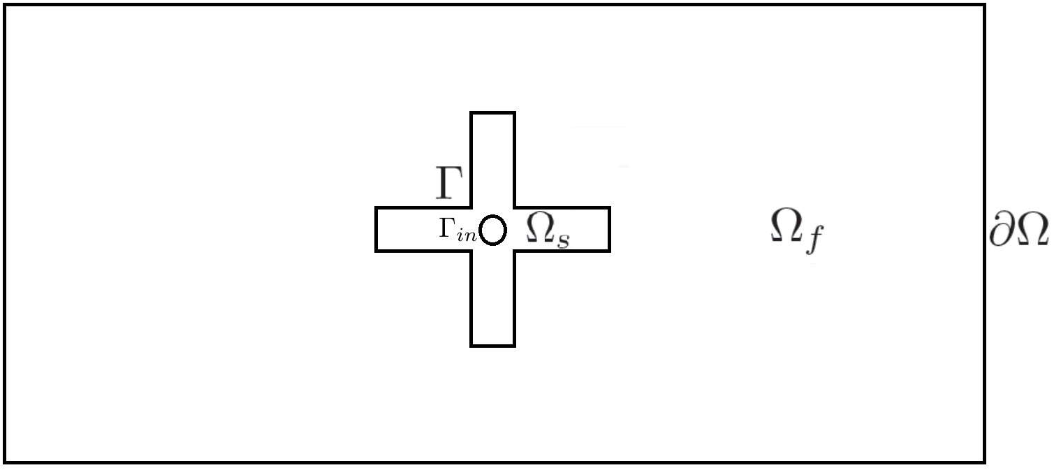
Figure 1: A schematic domain of FSI involving an elastic rotor $\Omega_{s}$ in 2D

As shown in Fig. 1, we consider an elastic rotor $\Omega_{s}(t)$ which is immersed in the fluid domain $\Omega_{f}(t)$, and spins around its rigid axis of rotation displayed as an inner circle $\Gamma_{in}$. $\Omega_{f}(t)\cap\Omega_{s}(t)=\emptyset$. Denote the whole domain as $\bar{\Omega}(t)=\bar{\Omega}_{f}(t)\cup\bar{\Omega}_{s}(t)\subset\mathbb{R}^{d}\ (d=2,3)$, and the interface of fluid and structure as $\Gamma(t)=\partial\Omega_{s}(t)\cap\partial\Omega_{f}(t)$. We use $\partial_{t}$ to denote the time derivative $\frac{\partial}{\partial t}$ in the rest of this paper.

For any position $\hat{\bm{x}}\in\hat{\Omega}=\Omega(0)$, we denote by $\bm{x}(\hat{\bm{x}},t)\in\Omega(t)$ its position at time $t$. $\bm{x}(\hat{\bm{x}},t)$ is usually called flow map. We can also use $\bm{x}(\hat{\bm{x}},t)$ to denote the flow map: $\hat{\bm{x}}\mapsto\bm{x}(\hat{\bm{x}},t)$. Then for given $t>0$, $\bm{x}(\cdot,t)$ is a diffeomorphism from $\Omega(0)$ to $\Omega(t)$. For $({\hat{\bm{x}}},t)\in\hat{\Omega}\times[0,T]$, we introduce the following variables in Lagrangian coordinates : the displacement $\hat{\bm{u}}({{\hat{\bm{x}}}},t)={\bm{x}}({\hat{\bm{x}}},t)-{\hat{\bm{x}}}$, and the velocity $\displaystyle\hat{\bm{v}}({\hat{\bm{x}}},t)=\partial_{t}\hat{\bm{u}}(\hat{\bm{x}},t)$. Using the relationship $\bm{x}=\bm{x}(\hat{\bm{x}},t)$, we also introduce the velocity in Eulerian coordinates: ${\bm{v}}({\bm{x}},t)=\hat{\bm{v}}({\hat{\bm{x}}},t)$. The symmetric part of the gradient of velocity is denoted by $\displaystyle\bm{\epsilon}(\bm{v})=(\nabla\bm{v}+(\nabla\bm{v})^{T})/2.$

For the sake of brevity of the notation, in the rest of this paper we omit the temporal variable $t$ in those notations which are defined in Eulerian coordinates, i.e., $\phi=\phi(t)$, and use $\hat{\phi}$ to denote those variables which are defined in Lagrangian coordinates, i.e., $\hat{\phi}=\phi(0)$ .

Fluid motion

The fluid is assumed to be Newtonian and incompressible. It is described by the following conservations of momentum and mass, i.e., Navier-Stokes equations, in terms of the fluid velocity $\bm{v}_{f}$ and pressure $p_{f}$ in Eulerian description.

$$\left\{\begin{aligned} \rho_{f}(\partial_{t}\bm{v}_{f}+\bm{v}_{f}\cdot\nabla\bm{v}_{f})&=\nabla\cdot\bm{\sigma}_{f}+\bm{g}_{f},&\quad\text{in }\Omega_{f},\\ \nabla\cdot\bm{v}_{f}&=0,&\quad\text{in }\Omega_{f},\\ \end{aligned}\right.$$ (1)

where

$$\bm{\sigma}_{f}=-p_{f}\bm{I}+2\mu_{f}\bm{\epsilon}(\bm{v}_{f}),$$

$\rho_{f}$ denotes the density of the fluid, $\mu_{f}$ the dynamic viscosity of the fluid, and $\bm{g}_{f}$ the external body force of the fluid.

Structure motion

The structure is assumed to be compressible. It is described by the following conservations of momentum and mass, i.e., the dynamic structure equations in terms of the structure velocity $\bm{v}_{s}$ in Eulerian description.

$$\left\{\begin{aligned} \rho_{s}(\partial_{t}\bm{v}_{s}+\bm{v}_{s}\cdot\nabla\bm{v}_{s})&=\nabla\cdot\bm{\sigma}_{s}+\bm{g}_{s},&\quad\text{in }\Omega_{s},\\ \partial_{t}\rho_{s}+\nabla\cdot(\rho_{s}\bm{v}_{s})&=0,&\quad\text{in }\Omega_{s},\\ \end{aligned}\right.$$ (2)

where $\rho_{s}$ denotes the density of the structure, and $\bm{g}_{s}$ the external body force of the structure. We define the Cauchy stress tensor of the structure $\bm{\sigma}_{s}$ as follows by changing variables for the structure equations from Eulerian coordinate to Lagrangian coordinate. We then have the following structure equation defined in Lagrangian system in terms of the structure displacement $\hat{\bm{u}}_{s}$ in the initial (reference) domain $\hat{\Omega}_{s}$.

$$\hat{\rho}_{s}\partial_{tt}\hat{\bm{u}}_{s} =\nabla\cdot(\bm{J}\bm{\sigma}_{s}\bm{F}^{-T})+\hat{\bm{g}}_{s}, \quad\text{in }\hat{\Omega}_{s}$$ (3)

where $\bm{F}({\hat{\bm{x}}},t)=\partial{\bm{x}}/\partial{\hat{\bm{x}}}=\bm{I}+\nabla_{{\hat{\bm{x}}}}\hat{\bm{u}}_{s}$ is the deformation gradient tensor, $\displaystyle\bm{J}({\hat{\bm{x}}},t)=det({\bm{F}}({\hat{\bm{x}}},t))$, $\hat{\rho}_{s}=\bm{J}\rho_{s}$, and $\hat{\bm{g}}_{s}=\bm{J}\bm{g}_{s}$. The derivation of (3) will be further shown in Section 3.

We introduce the first Piola-Kirchhoff stress tensor $\bm{P}_{s}$, defined as $\bm{P}_{s}=\bm{J}\bm{\sigma}_{s}\bm{F}^{-T}$, to simplify the stress form in (3). Further, $\bm{P}_{s}=\bm{F}\bm{S}$, where $\bm{S}$ is called the second Piola-Kirchhoff stress tensor, and thus defined as $\bm{S}=\bm{J}\bm{F}^{-1}\bm{\sigma}_{s}\bm{F}^{-T}$. Hence, the Cauchy stress tensor $\bm{\sigma}_{s}$ can be defined as

$$\bm{\sigma}_{s}(x)=\bm{J}^{-1}\bm{F}\bm{S}\bm{F}^{T},$$

which can be further specified based upon the constitutive law of a given structure material, i.e., its the second Piola-Kirchhoff stress tensor $\bm{S}$.

If we select the nonlinear St. Venant-Kirchhoff (STVK) material as the material of elastic rotor that is popularly adopted in the problems of hydro-turbine, wind-turbine and etc, we have the constitutive law of STVK material as follows [43, 38]

$$\bm{S}=2\mu_{s}\mathcal{E}+\lambda_{s}(tr\mathcal{E})\bm{I},$$

where, $\mathcal{E}$ is the Green-Lagrangian finite strain tensor, defined as

$$\mathcal{E}=(\bm{F}^{T}\bm{F}-\bm{I})/2=\frac{1}{2}\left(\nabla_{{\hat{\bm{x}}}}\hat{\bm{u}}_{s}+(\nabla_{{\hat{\bm{x}}}}\hat{\bm{u}}_{s})^{T}+(\nabla_{{\hat{\bm{x}}}}\hat{\bm{u}}_{s})^{T}\nabla_{{\hat{\bm{x}}}}\hat{\bm{u}}_{s}\right),$$

$\lambda_{s}=\frac{E\nu}{(1+\nu)(1-2\nu)}$ is the Lamé’s first parameter, and $\mu_{s}=\frac{E}{2(1+\nu)}$ is the shear modulus, here $E$ and $\nu$ denote the Young’s modulus and Poisson’s ratio, respectively. Hence, we can particularly define

$$\bm{\sigma}_{s}(x)=\frac{1}{\bm{J}}\bm{F}(2\mu_{s}\mathcal{E}+\lambda_{s}(tr\mathcal{E})\bm{I})\bm{F}^{T}.$$

Then, the structure equation (3) can be rewritten as the following form for STVK material, in particular.

$$\hat{\rho}_{s}\partial_{tt}\hat{\bm{u}}_{s}=\nabla\cdot(2\mu_{s}{\bm{F}}{\mathcal{E}}+\lambda_{s}(tr{\mathcal{E}}){\bm{F}})+\hat{\bm{g}}_{s}.$$ (4)

Apparently, (4) is a nonlinear equation. In Section 5, we will develop a linearized model, which is an approximation to (4) under the assumption of small deformation, specifically for a deformable structure undergoing a large rotation.

Interface conditions

Suppose the no-slip type boundary conditions hold on the interface of the fluid and structure, i.e., both velocity and normal stress are continuous across the interface $\Gamma$. The interface conditions on $\Gamma$ can be defined as follows in Eulerian description.

$$\bm{v}_{f}=\bm{v}_{s}=\partial_{t}\bm{u}_{s}, \text{on }\Gamma,$$ (5)

$$\bm{\sigma}_{f}\bm{n}_{f}+\bm{\sigma}_{s}\bm{n}_{s}=0, \text{on }\Gamma,$$ (6)

where $\bm{n}_{f}$ and $\bm{n}_{s}$ are the unit normal vector to the interface $\Gamma$ from the fluid and from the structure, respectively.

Boundary conditions

To fully define the boundary conditions other than the interface conditions, we split the outer boundary of fluid to two types: $\partial\Omega_{f}\backslash\Gamma=\Gamma_{D,f}\cup\Gamma_{N,f}$ and $\Gamma_{D,f}\cap\Gamma_{N,f}=\emptyset$, where, $\Gamma_{D,f}$ represents a part of the outer boundary of fluid on which Dirichlet boundary condition is imposed, and $\Gamma_{N,f}$ represents the rest part on which Neumann boundary condition is defined. Similarly, we split the outer boundary of structure as $\partial\hat{\Omega}_{s}\backslash\hat{\Gamma}=\hat{\Gamma}_{D,s}\cup\hat{\Gamma}_{N,s}$ and $\hat{\Gamma}_{D,s}\cap\hat{\Gamma}_{N,s}=\emptyset$.

The Dirichlet and Neumann boundary conditions for fluid and structure are given as follows

$$\bm{v}_{f}=\bm{v}_{D,f}, \text{on }\Gamma_{D,f},$$ (7)

$$\hat{\bm{u}}_{s}=\hat{\bm{u}}_{D,s}, \text{on }\hat{\Gamma}_{D,s},$$ (8)

$$\bm{\sigma}_{f}\bm{n}_{f}=\bm{g}_{N,f}, \text{on }\Gamma_{N,f},$$ (9)

$$\bm{\sigma}_{s}\bm{n}_{s}=\hat{\bm{g}}_{N,s}, \text{on }\hat{\Gamma}_{N,s}.$$ (10)

where, $\bm{v}_{D,f}(\bm{x},t),\ \hat{\bm{u}}_{D,s}(\hat{\bm{x}},t),\ \bm{g}_{N,f}(\bm{x},t),\ \hat{\bm{g}}_{N,s}(\hat{\bm{x}},t)$ are all prescribed. For example, Dirichlet boundary conditions for fluid can be the inflow boundary condition at the inlet and no-slip boundary condition on the wall. Dirichlet boundary conditions for structure can be used when it is clamped to the boundary. With $\bm{g}_{N,f}=0$, the Neumann boundary condition is adopted for fluid as the stress free boundary condition at the outlet of flow channel. Neumann boundary condition is employed for structure in FSI when the structure embraces the fluid inside and is imposed an external force on its outer boundary.

In our case studied in this paper, the structure is immersed in the fluid, thus Neumann boundary condition is not applied to the structure, i.e., $\hat{\Gamma}_{N,s}=\emptyset$. And, $\hat{\Gamma}_{D,s}=\Gamma_{in}$, on which $\hat{\bm{u}}_{D,s}$ is given if a rotation is prescribed. Later in this paper, we use the structure velocity, $\hat{\bm{v}}_{s}$, as the principle unknown instead of $\hat{\bm{u}}_{s}$, noting that $\hat{\bm{v}}_{s}=\partial_{t}\hat{\bm{u}}_{s}$. Then the corresponding Dirichlet boundary condition is changed as

$$\hat{\bm{v}}_{s}=\partial_{t}\hat{\bm{u}}_{D,s},\mbox{ on }\hat{\Gamma}_{D,s}.$$ (11)

Initial conditions

The following initial conditions hold for fluid and structure equations which are defined on the time interval $[0,T]$, with $T>0$.

$$\begin{array}[]{ll}\bm{v}_{f}(0)=\bm{v}^{0}_{f}(\bm{x}),&\text{in }\Omega_{f}\\ \hat{\bm{u}}_{s}(0)=\hat{\bm{u}}_{s}^{0}(\hat{\bm{x}}),\ \hat{\bm{v}}_{s}(0)=\hat{\bm{v}}_{s}^{0}(\hat{\bm{x}}),&\text{in }\hat{\Omega}_{s},\end{array}$$ (12)

where $\hat{\bm{u}}_{s}^{0}(\hat{\bm{x}})$, $\hat{\bm{v}}_{s}^{0}(\hat{\bm{x}})$, and $\bm{v}_{f}^{0}(\bm{x})$ are all prescribed.

3 Weak formulation of the FSI problem

Now we derive the weak formulations of the FSI problem. First, for any given domain $\Omega\subset\mathbb{R}^{d}$, we define the $H^{1}$ space of vector functions as

$${\mathbf{H}}^{1}(\Omega)=(H^{1}(\Omega))^{d}.$$

Moreover, define

$${\mathbf{H}}^{1}_{0}(\Omega_{f}) :=\{\bm{u}\in{\mathbf{H}}^{1}(\Omega_{f})|\bm{u}=0,\text{ on }\partial\Omega\cap\partial\Omega_{f}\},$$

$${\mathbf{H}}^{1}_{0}(\hat{\Omega}_{s}) :=\{\bm{u}\in{\mathbf{H}}^{1}(\hat{\Omega}_{s})|\bm{u}=0,\text{ on }\partial\hat{\Omega}\cap\partial\hat{\Omega}_{s}\},$$

$${\mathbf{H}}^{1}_{0}(\hat{\Omega}_{f}) :=\{\bm{u}\in{\mathbf{H}}^{1}(\hat{\Omega}_{f})|\bm{u}=0,\text{ on }\partial\hat{\Omega}\cap\partial\hat{\Omega}_{f}\}.$$

Let us define the following Sobolev spaces:

$$\mathbb{V} :=\{(\bm{v}_{f},\hat{\bm{v}}_{s})\in{\mathbf{H}}^{1}_{0}(\Omega_{f})\times{\mathbf{H}}^{1}_{0}(\hat{\Omega}_{s})\text{ such that }\bm{v}_{f}\circ\bm{x}(\hat{\bm{x}},t)=\hat{\bm{v}}_{s},\text{ on }\hat{\Gamma}\},$$ (13)

$$\mathbb{Q} :=L^{2}(\Omega_{f}).$$

In order to formulate the FSI problem weakly, we use test functions defined in $\Omega$, With the test function $\bm{\phi}\in(H_{0}^{1}(\Omega))^{d}$, we first write the weak formulations of the fluid and structure equations, respectively, as follows.

$$\int_{\Omega_{f}}\rho_{f}D_{t}\bm{v}_{f}\bm{\phi}d\bm{x}+\int_{\Omega_{f}}\bm{\sigma}_{f}:\bm{\epsilon}(\bm{\phi})d\bm{x}-\int_{\Gamma}\bm{\sigma}_{f}\bm{n}_{f}\cdot\bm{\phi}d\bm{x}=\int_{\Omega_{f}}\bm{g}_{f}\bm{\phi}d\bm{x},$$

$$\int_{\Omega_{s}}\rho_{s}D_{t}\bm{v}_{s}\bm{\phi}d\bm{x}+\int_{\Omega_{s}}{\bm{\sigma}}_{s}:\bm{\epsilon}(\bm{\phi})d\bm{x}-\int_{\Gamma}{\bm{\sigma}}_{s}\bm{n}_{s}\cdot\bm{\phi}d\bm{x}=\int_{\Omega_{s}}\bm{g}_{s}\bm{\phi}d\bm{x},$$

where $D_{t}\bm{\psi}=\partial_{t}\bm{\psi}+\bm{\psi}\cdot\nabla\bm{\psi}$.

We add up these two equations and cancel the boundary integral terms because of the interface condition (6), resulting in

$$\int_{\Omega_{f}}\rho_{f}D_{t}\bm{v}_{f}\bm{\phi}d\bm{x}+\int_{\Omega_{f}}\bm{\sigma}_{f}:\bm{\epsilon}(\bm{\phi})d\bm{x}+\int_{\Omega_{s}}\rho_{s}D_{t}\bm{v}_{s}\bm{\phi}d\bm{x}+\int_{\Omega_{s}}{\bm{\sigma}}_{s}:\bm{\epsilon}(\bm{\phi})d\bm{x}=\int_{\Omega_{f}}\bm{g}_{f}\bm{\phi}d\bm{x}+\int_{\Omega_{s}}\bm{g}_{s}\bm{\phi}d\bm{x}.$$

By a change of coordinates $\bm{x}=\bm{x}(\hat{\bm{x}},t),$ the stress term of structure part can be rewritten in Lagrangian coordinates

$$\int_{\Omega_{s}}{\bm{\sigma}}_{s}:\bm{\epsilon}(\bm{\phi})d\bm{x}=\int_{\hat{\Omega}_{s}}\hat{\bm{\sigma}}_{s}:\nabla_{\hat{\bm{x}}}\hat{\bm{\phi}}\bm{F}^{-1}\bm{J}d\hat{\bm{x}}=\int_{\hat{\Omega}_{s}}(\bm{J}\hat{\bm{\sigma}}_{s}\bm{F}^{-T}):\nabla_{\hat{\bm{x}}}\hat{\bm{\phi}}d\hat{\bm{x}},$$

where $\hat{\bm{\phi}}(\hat{\bm{x}},t)=\bm{\phi}(\bm{x}(\hat{\bm{x}},t),t)$ and $\hat{\bm{\sigma}}_{s}(\hat{\bm{x}},t)={\bm{\sigma}}_{s}(\bm{x}(\hat{\bm{x}},t),t)$. We also change the coordinates for the inertial term and the body force term, we then get the following weak form of FSI problem.

$$\int_{\Omega_{f}}\left(\rho_{f}D_{t}\bm{v}_{f}\bm{\phi}+\bm{\sigma}_{f}:\bm{\epsilon}(\bm{\phi})\right)d\bm{x}+\int_{\hat{\Omega}_{s}}\left(\hat{\rho}_{s}\partial_{tt}\hat{\bm{u}}_{s}\hat{\bm{\phi}}+\bm{P}_{s}:\nabla_{\hat{\bm{x}}}\hat{\bm{\phi}}\right)d\hat{\bm{x}}=\int_{\Omega_{f}}\bm{g}_{f}\bm{\phi}d\bm{x}+\int_{\hat{\Omega}_{s}}\hat{\bm{g}}_{s}\hat{\bm{\phi}}d\hat{\bm{x}},$$ (14)

which holds for any $\bm{\phi}\in\mathbb{V}$. Here, as shown in (3) in Section 2, we also derive the first Piola-Kirchhoff stress tensor $\bm{P}_{s}=\bm{J}\hat{\bm{\sigma}}_{s}\bm{F}^{-T}$, the density of the structure $\hat{\rho}_{s}(\hat{\bm{x}},t)=\bm{J}(\hat{\bm{x}},t)\rho_{s}(\bm{x}(\hat{\bm{x}},t),t)$, and the external body force $\hat{\bm{g}}_{s}(\hat{\bm{x}},t)=\bm{J}(\hat{\bm{x}},t)\bm{g}_{s}(\bm{x}(\hat{\bm{x}},t),t)$. By the conservation of mass, $\hat{\rho}_{s}$ is independent of $t$.

Thus, we are able to define the weak formulations of FSI as follows. Find $\bm{v}_{f}$, $p$ and $\hat{\bm{u}}_{s}$, satisfying (7), (8), and (12) such that for any given $t>0$, the following equations hold for any $(\bm{\phi},\hat{\bm{\phi}})\in\mathbb{V}$ and $q\in\mathbb{Q}$

$$\left\{\begin{aligned} (\hat{\rho}_{s}\partial_{tt}\hat{\bm{u}}_{s},\hat{\bm{\phi}})_{\hat{\Omega}_{s}}+\left(\rho_{f}D_{t}\bm{v}_{f},\bm{\phi}\right)_{\Omega_{f}}+(\bm{P}_{s}(\hat{\bm{u}}_{s}),\nabla\hat{\bm{\phi}})_{\hat{\Omega}_{s}}&+(\bm{\sigma}_{f},\bm{\epsilon}(\bm{\phi}))_{\Omega_{f}}\\ &=(\hat{\bm{g}}_{s},\hat{\bm{\phi}})+(\bm{g}_{f},\bm{\phi}),\\ (\nabla\cdot\bm{v}_{f},q)_{\Omega_{f}}&=0,\\ \bm{v}_{f}\circ\bm{x}(\hat{\bm{x}},t)&=\partial_{t}\hat{\bm{u}}_{s},\quad\text{on }\hat{\Gamma}.\\ \end{aligned}\right.$$ (15)

where, the pair $(\cdot,\cdot)_{\Omega}$ stands for the $L^{2}$-inner product on a domain $\Omega$, and $\nabla{\bm{\phi}}=\nabla_{\bm{x}}\bm{\phi},\ \nabla\hat{\bm{\phi}}=\nabla_{\hat{\bm{x}}}\hat{\bm{\phi}}$.

The above weak formulation shows that, on the continuous level, the continuity of velocity of fluid and structure across the interface is enforced in the definition of Sobolev space $\mathbb{V}$. However, on the discrete level, we only need one set of degrees of freedom of velocity to be shared by fluid and structure on the interface. To that end, first of all, a conforming mesh across the interface is needed, which is guaranteed by ALE method. Secondly, we need to merge the two sets of degrees of freedom of velocity arising from both fluid and structure on the interface to be one set only, which can be done by means of the so-called “Master-Slave Relation” technique. Thus, we no longer have any redundant degrees of freedom to eliminate, nor the need of Lagrange multiplier to enforce the continuity of velocity. We will further discuss this technique combining with ALE method in the next section.

4 Application of ALE method to the FSI problem

Due to the interaction between fluid and structure, we need to solve Navier-Stokes equations on a moving fluid domain. Re-meshing is always an option for a moving domain but it introduces extra computational cost and needs the interpolation to transfer the data between different time steps. Another frequently used approach is so-called the arbitrary Lagrangian-Eulerian (ALE) method, with which the moving fluid mesh sticks to the moving structure mesh and is updated by preserving the number of mesh nodes always the same, thus no interpolation occurs. The essential idea of ALE method is to formulate and solve the fluid problem on a deforming mesh, which deforms with the structure at the interface and then the fluid mesh is smoothed within the fluid domain. First introduced for finite element discretizations of the incompressible fluids in [30, 19], the ALE method provides an approach to find the fluid mesh that can fit the moving fluid domain $\Omega_{f}$. This mapping is a diffeomorphism on the continuous level, and we use piecewise polynomials to approximate it on the discrete level. We assume that the mesh motion is piecewise linear in the rest of this paper in order to make sure the updated mesh by ALE mapping remains a undistorted triangular mesh.

We denote the image of $\hat{\Omega}_{f}$ under the piecewise linear map $\bm{x}_{h,f}$ by $\Omega_{f}^{n}$. $\Omega_{f}^{n}$ is triangulated by a moving mesh with respect to time, denoted by $T_{h}(\Omega_{f}^{n})$. Note that $\Omega_{f}^{n}$ is assumed to be a polygonal domain in 2D, and a polyhedral domain in 3D. There are two main ingredients in the ALE approach:

1. Define how the grid is moving with respect to time such that it matches the structure displacement at the fluid-structure interface.

2. Define how the material derivatives are discretized on the moving grid.

Given the structure trajectory $\bm{x}(\hat{\bm{x}},t)$ defined on $\hat{\Gamma},$ the moving grid can be described by a diffeomorphism $\mathcal{A}(\cdot,t):\hat{\Omega}_{f}\mapsto\Omega_{f}$ that satisfies

$$\left\{\begin{aligned} \mathcal{A}(\hat{\bm{x}},t)&=\hat{\bm{x}},&\text{ on }&\partial\hat{\Omega}_{f}\cap\partial\hat{\Omega},\\ \mathcal{A}(\hat{\bm{x}},t)&=\bm{x}(\hat{\bm{x}},t),&\text{ on }&\hat{\Gamma}.\\ \end{aligned}\right.$$ (16)

ALE mappings satisfying (16) are by no means unique. In the interior of $\hat{\Omega}_{f}$, the ALE mapping can be “arbitrary”. One popular approach to uniquely determine $\mathcal{A}$ is to solve a partial differential equation

$$\mathcal{L}\mathcal{A}=0,\quad\mbox{in }\hat{\Omega}_{f}.$$ (17)

A popular choice for the operator $\mathcal{L}$ is the Laplacian, $\mathcal{L}=-\Delta$. For more choices of formulating the ALE mapping equation, we refer to [10, 19] and references therein.

With the ALE technique, we can reformulate the fluid momentum equation on a moving fluid domain as follows

$$\rho_{f}\partial^{\mathcal{A}}_{t}\bm{v}_{f}+\rho_{f}((\bm{v}_{f}-\bm{w})\cdot\nabla)\bm{v}_{f}=\nabla\cdot\bm{\sigma}_{f}+\bm{g}_{f},$$ (18)

where, $\bm{w}=\partial_{t}\mathcal{A}\circ\mathcal{A}^{-1}$ denotes the velocity of fluid mesh, and

$$\partial^{\mathcal{A}}_{t}\bm{v}_{f}|_{(\bm{x},t)}:=\partial_{t}\bm{v}_{f}+(\bm{w}\cdot\nabla)\bm{v}_{f}$$

is called ALE material derivative.

In particular, we define the discretization of the ALE material derivative on the moving grid as follows

$$\partial^{\mathcal{A}}_{t}\bm{v}_{f}\approx\frac{\bm{v}_{f}(\bm{x},t_{n})-\bm{v}_{f}(\mathcal{A}_{n-1}\circ A_{n}^{-1}(\bm{x}),t_{n-1})}{\Delta t},$$ (19)

where, $\mathcal{A}_{n-1}\circ\mathcal{A}_{n}^{-1}(\bm{x})$ is the location of $\bm{x}$ at $t=t_{n-1}$ before it is moved by ALE mesh motion. For example, if $\mathcal{A}\circ\mathcal{A}_{n}^{-1}(\bm{x})$ is a mesh node at $t=t_{n-1}$, the ALE mesh motion moves it to $\bm{x}$ at $t=t_{n}$, which is a mesh node at $t=t_{n}$. Thus the interpolation between the meshes on different time levels is avoided.

In order to precisely fulfill the kinematic interface condition (5) and apply the Master-Slave Relation, we need to reformulate the structure equation in terms of the structure velocity $\hat{\bm{v}}_{s}$ instead of its displacement $\hat{\bm{u}}_{s}$ in (15). We use the following relation of $\hat{\bm{v}}_{s}$ and $\hat{\bm{u}}_{s}$

$$\hat{\bm{v}}_{s}=\partial_{t}\hat{\bm{u}}_{s},\,\text{ or },\,\hat{\bm{u}}_{s}=\hat{\bm{u}}_{s}^{0}+\int_{0}^{t}\hat{\bm{v}}_{s}(\tau)d\tau$$ (20)

to reformulate (15), and rewrite the kinematic condition (5) in reference configuration as

$$\hat{\bm{v}}_{s}({\hat{\bm{x}}})=\bm{v}_{f}(\mathcal{A}({\hat{\bm{x}}},t)),\quad\text{on}\ \hat{\Gamma}.$$

Thus the Master-Slave Relation can be efficiently applied since both master and slave DOFs are simply equal to each other at the same mesh node on the interface. In addition, we introduce an equivalent ALE mapping for the displacement of fluid mesh $\mathcal{A}_{\bm{u}}(\hat{\bm{x}},t)=\mathcal{A}(\hat{\bm{x}},t)-\hat{\bm{x}}(\hat{\bm{x}},t)$, satisfying

$$-\Delta\mathcal{A}_{\bm{u}} =0, \text{ in }\hat{\Omega}_{f}$$ (21)

$$\mathcal{A}_{\bm{u}} =0, \text{ on }\partial\hat{\Omega}_{f}\cap\partial\hat{\Omega},$$ (22)

$$\mathcal{A}_{\bm{u}} =\hat{\bm{u}}_{s}, \text{ on }\hat{\Gamma}.$$ (23)

The resulted new weak formulation is thus defined as follows with ALE mapping, the structure velocity $\hat{\bm{v}}_{s}$ in the structure equation, and ALE material derivative in the fluid equation. Find $\bm{v}_{f},\hat{\bm{v}}_{s},p,\mathcal{A}_{\bm{u}}$, satisfying (5), (7), (11) and (12), such that for any given $t>0$, the following system of equations hold for $\forall(\hat{\bm{\phi}},\bm{\phi})\in\mathbb{V},q\in\mathbb{Q},\xi\in{\mathbf{H}}^{1}_{0}(\hat{\Omega}_{f})$

$$\left\{\begin{aligned} (\hat{\rho}_{s}\partial_{t}\hat{\bm{v}}_{s},\hat{\bm{\phi}})_{\hat{\Omega}_{s}}+({\bm{P}}_{s}(\hat{\bm{u}}_{s}^{0}+\int_{0}^{t}\hat{\bm{v}}_{s}(\tau)d\tau),\nabla\hat{\bm{\phi}})_{\hat{\Omega}_{s}}&+(\rho_{f}\partial^{\mathcal{A}}_{t}{\bm{v}}_{f},\bm{\phi})_{\Omega_{f}}\\ +(\rho_{f}({\bm{v}}_{f}-\bm{w})\cdot\nabla{\bm{v}}_{f},\bm{\phi})_{\Omega_{f}}+({\bm{\sigma}}_{f},\bm{\epsilon}(\bm{\phi}))_{\Omega_{f}}&=(\hat{\bm{g}}_{s},\hat{\bm{\bm{\phi}}})+(\bm{g}_{f},\bm{\bm{\phi}}),\\ (\nabla\cdot{\bm{v}}_{f},q)_{\Omega_{f}}&=0,\\ (\nabla\mathcal{A}_{\bm{u}},\nabla\xi)_{\hat{\Omega}_{f}}&=0,\\ \mathcal{A}_{\bm{u}}&=\hat{\bm{u}}_{s}^{0}+\int_{0}^{t}\hat{\bm{v}}_{s}(\tau)d\tau,\mbox{ on }\hat{\Gamma}.\\ \end{aligned}\right.$$ (24)

For the simplicity of notation, in what follows, we suppose $\bm{g}_{f}=\hat{\bm{g}}_{s}=0$ by assuming no external body force is acted on the fluid and structure.

5 Remodeling of the rotational elastic structure

In this section, we attempt to develop a new model for an elastic rotor with large rotation and small deformation, which, simultaneously, is suitable for the implementation of ALE method for FSI problems which involve the rotation as well as the deformation in the structure.

From (4) we know that the equation of an elastic structure that follows the constitutive law of STVK material and is spinning around the axis of rotation, $\Gamma_{in}$, is specifically defined as

$$\hat{\rho}_{s}\partial_{tt}\hat{\bm{u}}_{s}=\nabla\cdot\bm{P}_{s}=\nabla\cdot(\lambda_{s}(tr{\mathcal{E}}){\bm{F}}+2\mu_{s}{\bm{F}}{\mathcal{E}})$$ (25)

with the following boundary condition

$$\hat{\bm{u}}_{s}={\bm{x}}-{{\hat{\bm{x}}}}=(R(\theta)-{\bm{I}})({{\hat{\bm{x}}}}-\hat{\bm{x}}_{0}),~{}~{}\mbox{ on }\Gamma_{in},$$ (26)

where $R(\theta)$ is the rotational matrix depending on the angle of rotation $\theta(t)$. For instance, let us specify a case in which the axis of rotation is $z$-axis, then

$$R(\theta)=\left(\begin{array}[]{rrr}\cos\theta&-\sin\theta&0\\ \sin\theta&\cos\theta&0\\ 0&0&1\\ \end{array}\right).$$ (27)

For the sake of brevity, in what follows, we just use $R$ to denote the rotational matrix.

Here we consider a hyperelastic structure such as the SVTK material for which the deformation can be still small while a large rotation occurs. The key idea is that we can decompose the structure motion into the rotational part and the deformation part [47, 21]. Suppose ${{\hat{\bm{x}}}}_{0}$ is a point on the axis of rotation, we can decompose the trajectory of each material particle as follows by using the rotational matrix $R$ arising from the boundary condition (26),

$${\bm{x}}-{{\hat{\bm{x}}}}_{0}=R({{\hat{\bm{x}}}}+\hat{\bm{u}}_{d}-{{\hat{\bm{x}}}}_{0}),$$ (28)

where $\hat{\bm{u}}_{d}$ is the local deformation displacement in the reference configuration, it does not contain any information of the rotation, thus $\hat{\bm{u}}_{d}=0$ on $\Gamma_{in}$. Hence, the total structure displacement, $\hat{\bm{u}}_{s}$, can be decomposed as

$$\hat{\bm{u}}_{s}={\bm{x}}-{{\hat{\bm{x}}}}=(R-{\bm{I}})({{\hat{\bm{x}}}}-\hat{\bm{x}}_{0})+R\hat{\bm{u}}_{d}=\hat{\bm{u}}_{\theta}+R\hat{\bm{u}}_{d},$$ (29)

where $\hat{\bm{u}}_{\theta}=(R-{\bm{I}})({{\hat{\bm{x}}}}-{{\hat{\bm{x}}}}_{0})$ is referred to as the rotational part of the structure displacement.

From (28) we obtain the deformation gradient tensor ${\bm{F}}=R({\bm{I}}+{\mathbf{H}}),\text{ where }{\mathbf{H}}=\nabla\hat{\bm{u}}_{d}$. Then, the Green-Lagrangian finite strain tensor ${\mathcal{E}}=({\bm{F}}^{T}{\bm{F}}-{\bm{I}})/2=({\mathbf{H}}+{\mathbf{H}}^{T}+{\mathbf{H}}^{T}{\mathbf{H}})/2.$ Thus the first Piola-Kirchhoff stress in (25), $\bm{P}_{s}={\bm{F}}(\lambda_{s}(tr{\mathcal{E}})\bm{I}+2\mu_{s}{\mathcal{E}})$, leads to a function of ${\mathbf{H}}$ as follows

$$\bm{P}_{s}({\mathbf{H}})=R({\bm{I}}+{\mathbf{H}})\left(\frac{\lambda_{s}}{2}tr({\mathbf{H}}+{\mathbf{H}}^{T}+{\mathbf{H}}^{T}{\mathbf{H}})\bm{I}+\mu_{s}({\mathbf{H}}+{\mathbf{H}}^{T}+{\mathbf{H}}^{T}{\mathbf{H}})\right).$$

Since we only consider a small deformation, i.e. ${\mathbf{H}}\approx 0$, we then conduct a linear approximation for the above equation by Taylor expansion around the non-deformable configuration ${\mathbf{H}}=0$, resulting in

$$\bm{P}_{s}\approx\frac{1}{2}\lambda_{s}R((tr{\mathbf{H}})\bm{I}+(tr{\mathbf{H}}^{T})\bm{I})+\mu_{s}R({\mathbf{H}}+{\mathbf{H}}^{T})=R(\lambda_{s}tr(\epsilon(\hat{\bm{u}}_{d})){\bm{I}}+2\mu_{s}\epsilon(\hat{\bm{u}}_{d})),$$ (30)

where $\epsilon(\hat{\bm{u}}_{d})=(\nabla\hat{\bm{u}}_{d}+(\nabla\hat{\bm{u}}_{d})^{T})/2$ is the linear approximation of ${\mathcal{E}}(\hat{\bm{u}}_{d})$. Therefore, we attain the linear approximation for the stress tensor in Lagrangian description,

$$\hat{\bm{\sigma}}_{s}=\bm{P}_{s}\approx R(\lambda_{s}tr(\epsilon(\hat{\bm{u}}_{d})){\bm{I}}+2\mu_{s}\epsilon(\hat{\bm{u}}_{d})).$$

We may equivalently rewrite $\hat{\bm{\sigma}}_{s}=R{\bm{D}}\epsilon(\hat{\bm{u}}_{d})$, where ${\bm{D}}_{ijkl}=2\mu_{s}\delta_{ik}\delta_{jl}+\lambda_{s}\delta_{ij}\delta_{kl}$ is a fourth order tensor and ${\bm{D}}\epsilon(\hat{\bm{u}}_{d})$ is the contraction of ${\bm{D}}$ and $\epsilon(\hat{\bm{u}}_{d})$, i.e. $({\bm{D}}\epsilon(\hat{\bm{u}}_{d}))_{ij}=\sum_{kl}{\bm{D}}_{ijkl}(\epsilon(\hat{\bm{u}}_{d}))_{kl}.$

Thus, (25) is approximated by

$$\hat{\rho}_{s}\partial_{tt}\hat{\bm{u}}_{s}=\nabla\cdot\left(R(\lambda_{s}tr(\epsilon(\hat{\bm{u}}_{d})){\bm{I}}+2\mu_{s}\epsilon(\hat{\bm{u}}_{d}))\right)=\nabla\cdot(R{\bm{D}}\epsilon(\hat{\bm{u}}_{d})),$$ (31)

which can be treated as a linear elasticity model of the elastic rotor, noting that the right hand side of (31) is linear with respect to $\hat{\bm{u}}_{d}$.

Next, we reformulate (31) in terms of an unique principle unknown $\hat{\bm{u}}_{s}$. Due to (29), we have $R\hat{\bm{u}}_{d}=\hat{\bm{u}}_{s}-\hat{\bm{u}}_{\theta}$, thus $\epsilon(\hat{\bm{u}}_{d})=\epsilon(R^{T}\hat{\bm{u}}_{s})-\epsilon(R^{T}\hat{\bm{u}}_{\theta})$. Note that $\hat{\bm{u}}_{\theta}=(R-{\bm{I}})({{\hat{\bm{x}}}}-{{\hat{\bm{x}}}}_{0})$, then ${\bm{D}}\epsilon(R^{T}\hat{\bm{u}}_{\theta})={\bm{D}}\epsilon((\bm{I}-R^{T})(\hat{\bm{x}}-{{\hat{\bm{x}}}}_{0}))$. Therefore, we attain the following equation of the elastic structure in terms of $\hat{\bm{u}}_{s}$ only,

$$\hat{\rho}_{s}\partial_{tt}\hat{\bm{u}}_{s}-\nabla\cdot(R{\bm{D}}\epsilon(R^{T}\hat{\bm{u}}_{s})) = -\nabla\cdot(R{\bm{D}}\epsilon((R^{T}-\bm{I})(\hat{\bm{x}}_{0}-\hat{\bm{x}}))).$$ (32)

It is assumed that the structure only rotates on the axis of rotation, i.e., the inner boundary $\Gamma_{in}$. Then, with a given rotational matrix $R$, the admissible solution set for $\hat{\bm{u}}_{s}$ is defined as follows

$${\mathbf{H}}_{R}^{1}(\hat{\Omega}_{s})=\{\hat{\bm{u}}\in{\mathbf{H}}^{1}(\hat{\Omega}_{s})|\hat{\bm{u}}(\hat{\bm{x}})=(R-\bm{I})(\hat{\bm{x}}-\hat{\bm{x}}_{0}),~{}\hat{\bm{x}}\in\Gamma_{in}\}.$$

By (29), $\hat{\bm{u}}\in{\mathbf{H}}_{R}^{1}(\hat{\Omega}_{s})$ can be decomposed into the rotational part $\hat{\bm{u}}_{\theta}=(R-{\bm{I}})({{\hat{\bm{x}}}}-{{\hat{\bm{x}}}}_{0})$ and the deformation part $\hat{\bm{u}}_{d}\in{\mathbf{H}}^{1}_{0}(\hat{\Omega}_{s})$ such that

$$\hat{\bm{u}}=R\hat{\bm{u}}_{d}+(R-\bm{I})(\hat{\bm{x}}-\hat{\bm{x}}_{0}).$$ (33)

It is obvious that given any $\hat{\bm{u}}\in{\mathbf{H}}_{R}^{1}(\hat{\Omega}_{s})$, there exists a unique $\hat{\bm{u}}_{d}\in{\mathbf{H}}_{0}^{1}(\hat{\Omega}_{s})$ such that (33) holds.

Assume that $R$ is given for $t\in[0,T]$, then the weak formulation of (32) can be defined as follows, $\forall t\in[0,T]$, find $\hat{\bm{u}}_{s}(t)\in{\mathbf{H}}_{R}^{1}(\hat{\Omega}_{s})$ such that $\forall\hat{\bm{\phi}}\in({H}_{0}^{1}(\hat{\Omega}_{s}))^{d}$

$$\noindent(\hat{\rho}_{s}\partial_{tt}\hat{\bm{u}}_{s},\hat{\bm{\phi}})_{\hat{\Omega}_{s}}+({\bm{D}}\epsilon(R^{T}\hat{\bm{u}}_{s}),\epsilon(R^{T}\hat{\bm{\phi}}))_{\hat{\Omega}_{s}}=({\bm{D}}\epsilon((\bm{I}-R^{T})({{\hat{\bm{x}}}}-\hat{\bm{x}}_{0})),\epsilon(R^{T}\hat{\bm{\phi}}))_{\hat{\Omega}_{s}}+\int_{\hat{\Gamma}}\bm{g}_{inf}\hat{\bm{\phi}}\ ds,$$ (34)

where, the stiffness term on the left hand side of (34) is symmetric positive definite, and $\bm{g}_{inf}$ on the right hand side is the interface force from fluid, which will be canceled in the weak form of FSI due to the continuity of normal stress on the interface of fluid and structure. We conclude that the weak formulation (34) can also be derived based on the linear elasticity equation on the rotational configuration, as demonstrated at below.

Let $\hat{\Omega}$ be the reference configuration of elasticity. Suppose the material undergoes a large rotation along with a small deformation. At time $t$, the rotational matrix is given as $R$. Without loss of generality, let $\hat{\bm{x}}_{0}=0$. Define

$$\hat{\Omega}_{R}:=\{\hat{\bm{x}}_{R}=R\hat{\bm{x}},\hat{\bm{x}}\in\hat{\Omega}\},$$

which is the rotational configuration. It is known that when formulating the equation in $\hat{\Omega}_{R}$, we can just use the linear elasticity. When formulating the equation on $\hat{\Omega}$, however, the linearization is more complicated. Now we want to show that we can obtain the same equation by formulating it in different configurations.

Recall the decomposition of displacement in $\hat{\Omega}$:

$$\hat{\bm{u}}_{s}=(R-\bm{I})\hat{\bm{x}}+R\hat{\bm{u}}_{d}=\hat{\bm{u}}_{\theta}+\hat{\bm{u}}_{R},$$

where, $\hat{\bm{u}}_{R}:=R\hat{\bm{u}}_{d}$ is the unknown of the linear elasticity equation defined in $\hat{\Omega}_{R}$. Note that we use the subscript $R$ for the variables defined in $\hat{\Omega}_{R}$, and subscript free for those variables defined in $\hat{\Omega}$. To simplify the notation, we do not distinguish between $f(\hat{\bm{x}})$ and $f(R\hat{\bm{x}})$.

First, we look at the stress term in the weak form,

$$\left(2\mu_{s}\epsilon_{R}(\hat{\bm{u}}_{R})+\lambda_{s}tr(\epsilon_{R}(\hat{\bm{u}}_{R}))\bm{I},\nabla_{R}\bm{\phi}\right)_{\hat{\Omega}_{R}}$$

$$= \left(\mu_{s}(\nabla_{R}\hat{\bm{u}}_{R}+(\nabla_{R}\hat{\bm{u}}_{R})^{T})+\lambda_{s}tr(\nabla_{R}\hat{\bm{u}}_{R}+(\nabla_{R}\hat{\bm{u}}_{R})^{T})\bm{I}/2,\nabla_{R}\bm{\phi}\right)_{\hat{\Omega}_{R}}$$

$$= \left(\mu_{s}(\nabla\hat{\bm{u}}_{R}R^{T}+(\nabla\hat{\bm{u}}_{R}R^{T})^{T})+\lambda_{s}tr(\nabla\hat{\bm{u}}_{R}R^{T}+(\nabla\hat{\bm{u}}_{R}R^{T})^{T})\bm{I}/2,\nabla\bm{\phi}R^{T}\right)_{\hat{\Omega}}$$

$$= \left(\mu_{s}(\nabla\hat{\bm{u}}_{R}+R(\nabla\hat{\bm{u}}_{R})^{T}R)+\lambda_{s}tr(R^{T}\nabla\hat{\bm{u}}_{R}+(R^{T}\nabla\hat{\bm{u}}_{R})^{T})R/2,\nabla\bm{\phi}\right)_{\hat{\Omega}}$$

$$= \left(R[\mu_{s}(\nabla(R^{T}\hat{\bm{u}}_{R})+(\nabla(R^{T}\hat{\bm{u}}_{R}))^{T})+\lambda_{s}tr(\nabla(R^{T}\hat{\bm{u}}_{R})+(\nabla(R^{T}\hat{\bm{u}}_{R}))^{T})\bm{I}/2],\nabla\bm{\phi}\right)_{\hat{\Omega}}$$

$$= \left(R[2\mu\epsilon(\hat{\bm{u}}_{d})+\lambda_{s}tr(\epsilon(\hat{\bm{u}}_{d}))\bm{I}],\nabla\bm{\phi}\right)_{\hat{\Omega}}.$$

This stress term is the same as that shown in (31). Meanwhile, we have the following inertia term in the rotational configuration

$$(\hat{\rho}_{s}\partial_{tt}\hat{\bm{u}}_{R},\bm{\phi})_{\Omega_{R}}.$$

Because the rotational configuration is a non-inertial reference frame, for the sake of force equilibrium, the following centrifugal force shall be added to the equation

$$(\hat{\rho}_{s}\partial_{tt}\hat{\bm{u}}_{\theta},\bm{\phi})_{\Omega_{R}}.$$

Thus we can recover the inertia term in (34) given that

$$(\hat{\rho}_{s}\partial_{tt}\hat{\bm{u}}_{R},\bm{\phi})_{\Omega_{R}}+(\hat{\rho}_{s}\partial_{tt}\hat{\bm{u}}_{\theta},\bm{\phi})_{\Omega_{R}}=(\hat{\rho}_{s}\partial_{tt}\hat{\bm{u}}_{s},\bm{\phi})_{\hat{\Omega}}.$$

We have, therefore, shown the equivalence with the derivation of the equation (34).

After updating the structure equation with the linear elasticity involving the rotation, we have the following new weak formulation of the FSI system with a rotational elastic structure. Find $\bm{v}_{f},\hat{\bm{v}}_{s},p,\mathcal{A}_{\bm{u}}$, satisfying (5), (7), (11), and (12), such that for any given $t>0$, the following equations hold for $\forall(\hat{\bm{\phi}},\bm{\phi})\in\mathbb{V},q\in\mathbb{Q},\xi\in{\mathbf{H}}^{1}_{0}(\hat{\Omega}_{f})$

$$\left\{\begin{aligned} (\hat{\rho}_{s}\partial_{t}\hat{\bm{v}}_{s},\hat{\bm{\phi}})_{\hat{\Omega}_{s}}+({\bm{D}}\epsilon(R^{T}(\hat{\bm{u}}_{s}^{0}+\int_{0}^{t}\hat{\bm{v}}_{s}(\tau)d\tau)),\epsilon(R^{T}\hat{\bm{\phi}}))_{\hat{\Omega}_{s}}&+(\rho_{f}\partial^{\mathcal{A}}_{t}{\bm{v}}_{f},\bm{\phi})_{\Omega_{f}}\\ +(\rho_{f}({\bm{v}}_{f}-\bm{w})\cdot\nabla{\bm{v}}_{f},\bm{\phi})_{\Omega_{f}}+({\bm{\sigma}}_{f},\bm{\epsilon}(\bm{\phi}))_{\Omega_{f}}&=({\bm{D}}\epsilon((\bm{I}-R^{T})({{\hat{\bm{x}}}}-\hat{\bm{x}}_{0})),\epsilon(R^{T}\hat{\bm{\phi}}))_{\hat{\Omega}_{s}},\\ (\nabla\cdot{\bm{v}}_{f},q)_{\Omega_{f}}&=0,\\ (\nabla\mathcal{A}_{\bm{u}},\nabla\xi)_{\hat{\Omega}_{f}}&=0,\\ \mathcal{A}_{\bm{u}}&=\hat{\bm{u}}_{s}^{0}+\int_{0}^{t}\hat{\bm{v}}_{s}(\tau)d\tau,\mbox{ on }\hat{\Gamma}.\\ \end{aligned}\right.$$ (35)

6 The modified ALE method for an elastic rotor immersed in the fluid

In this section, we develop a modified ALE method to deal with the elastic rotor that is immersed in a non-axisymmetric fluid domain. Roughly speaking, we first introduce an artificial cylindrical buffer zone $\Omega_{rf}$ in the fluid domain which embraces the elastic rotor $\Omega_{s}$ inside and rotates together on the same axis of rotation and with the same angular velocity, and name the remaining region in $\Omega_{f}$ as the stationary fluid subdomain, denoted by $\Omega_{sf}$, thus $\Omega_{f}=\Omega_{sf}\cup\Omega_{rf}$. Denote the interface between $\Omega_{rf}$ and $\Omega_{sf}$ by $\Gamma_{rs}$, i.e., $\Gamma_{rs}=\partial\Omega_{rf}\cap\partial\Omega_{sf}$. On the other hand, we measure the relative motion of each pair of mesh nodes on $\Gamma_{rs}$, and add up the difference of motion to the mesh nodes on $\partial\Omega_{rf}$. Thus, the mesh in $\bar{\Omega}_{rf}$ needs to be updated all the time in the numerical computation in order to conform with the mesh in $\Omega_{s}$ through the interface of $\Omega_{rf}$ and $\Omega_{s}$, $\Gamma$, and with the mesh in $\Omega_{sf}$ through the interface $\Gamma_{rs}$ , as shown in Fig. 2.

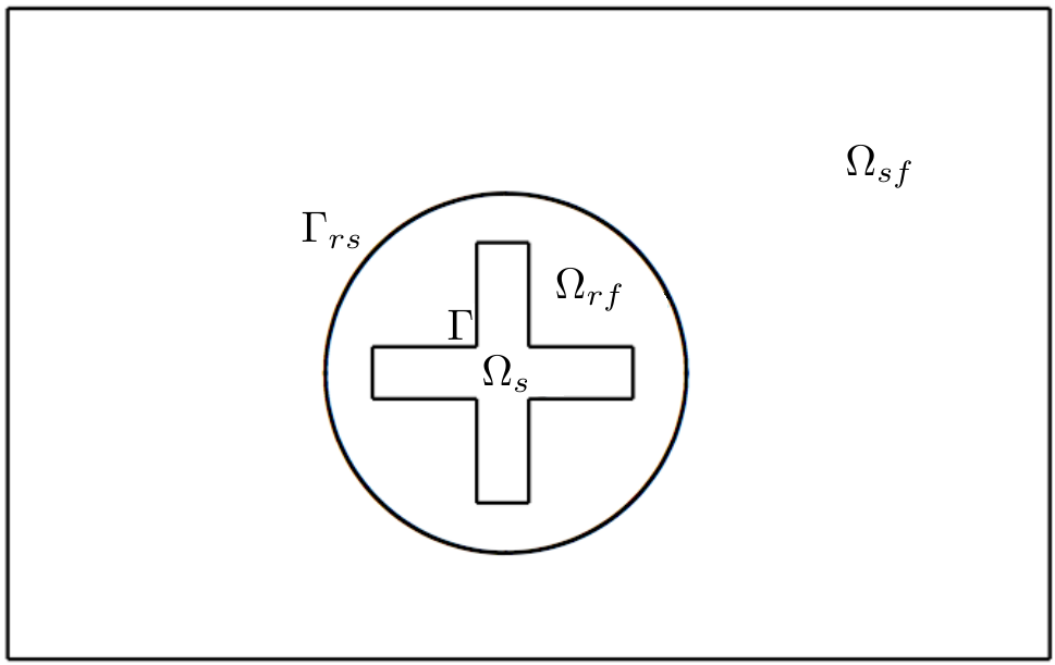
Figure 2: The cylindrical buffer zone $\Omega_{rf}$ that embraces an elastic rotor $\Omega_{s}$

For the sake of brevity, we use a 2D example to show the idea of how to use ALE method to generate the fluid mesh in fluid domain $\Omega_{f}$. Different from the traditional ALE approach, the modified ALE method only moves the mesh nodes in the rotational fluid buffer zone $\Omega_{rf}$. We handle the fluid mesh motion in a similar fashion as we do for the structure, i.e., decomposing the displacement to the rotational part and the deformation part: $\hat{\bm{u}}_{s}=\hat{\bm{u}}_{\theta}+R\hat{\bm{u}}_{d}$. In particular, we decompose $\mathcal{A}_{\bm{u}}$, the displacement of the rotational fluid mesh defined in $\hat{\Omega}_{rf}$, into two parts: the rotational part $\hat{\bm{u}}_{\theta}$ and the deformation part $\mathcal{A}_{D}$, i.e.,

$$\mathcal{A}_{\bm{u}}=\hat{\bm{u}}_{\theta}+\mathcal{A}_{D},$$

where, $\hat{\bm{u}}_{\theta}=(R-{\bm{I}})({{\hat{\bm{x}}}}-{{\hat{\bm{x}}}}_{0})$ is the rotational displacement of the mesh which is determined by the given rotational matrix, $R$, defined on the axis of rotation $\Gamma_{in}$. In addition, we also need the rotational fluid mesh to be conforming with the rotational and deformable structure mesh from inside, and with the stationary fluid mesh from outside. The deformation displacement, $\mathcal{A}_{D}$, serves on this purpose by moving the mesh according to the structure deformation displacement, $\hat{\bm{u}}_{s}-\hat{\bm{u}}_{\theta}$, on the interface $\hat{\Gamma}$, and by locally moving the mesh nodes on the interface $\hat{\Gamma}_{rs}:=\partial\hat{\Omega}_{rf}\cap\partial\hat{\Omega}_{sf}$ to properly match with the stationary fluid mesh. Namely, we let $\mathcal{A}_{D}$ satisfy the following modified ALE mapping

$$\left\{\begin{aligned} -\Delta\mathcal{A}_{D}&=0,&\mbox{in }\hat{\Omega}_{rf},\\ \mathcal{A}_{D}&=\hat{\bm{u}}_{s}-\hat{\bm{u}}_{\theta},&\mbox{on }\hat{\Gamma},\\ \mathcal{A}_{D}&=\hat{\bm{u}}_{m},&\mbox{on }\hat{\Gamma}_{rs},\\ \end{aligned}\right.$$ (36)

where, $\hat{\bm{u}}_{m}$ needs to be defined such that each sliding mesh node on $\hat{\Gamma}_{rs}$ from the side of $\hat{\Omega}_{rf}$ matches with a fixed mesh node on $\hat{\Gamma}_{rs}$ from the other side of $\hat{\Omega}_{sf}$ by locally moving for such amount of displacement $\hat{\bm{u}}_{m}$ on $\hat{\Gamma}_{rs}$.

Now using Fig. 3 we illustrate how to find such small displacement $\hat{\bm{u}}_{m}$ in two dimensional case. The interface is locally shown as a straight line just for an illustration purpose. In practice, the curved interface is approximated by piecewise line segments in 2D or piecewise triangular slice in 3D. The technique shown here is applicable to the general cases with piecewise line segments/triangular slices.

Figure 3: Re-matching grid points on the interface of $\Omega_{rf}$

Let $\{N_{i}^{r}\}_{i=0}^{m-1}$ be coordinates of boundary nodes from $\partial\Omega_{rf}$ and $\{N_{i}^{st}\}_{i=0}^{m-1}$ the counterpart from $\partial\Omega_{sf}$. After $\Omega_{rf}$ is rotated, we assume $N_{0}^{r}$ falls in between $N_{K-1}^{st}$ and $N_{K}^{st}$. Then we can choose the following mapping between the nodes:

$$N_{i}^{r}\mapsto N_{[K+i]_{m}}^{st}.$$

Here $[m]_{n}$ denotes the modulo operation. $\hat{\bm{u}}_{m}$ can be correspondingly defined on $\{N_{i}^{r}\}$:

$$\hat{\bm{u}}_{m}(x)=N_{[K+i]_{m}}^{st}-N_{i}^{r},\quad\mbox{if }x=N_{i}^{r}.$$

On $\hat{\Gamma}\backslash\{N_{i}^{r}\}$, $\hat{\bm{u}}_{m}$ is defined by linear interpolation of the nodal values. Since each boundary node from $\partial\Omega_{rf}$ has a nearby node from $\partial\Omega_{sf}$ to match, the magnitude of $\hat{\bm{u}}_{m}$ is bounded by mesh diameter. Therefore it will not cause problems for ALE mapping. Note that it is also possible to match $N_{i}^{r}$ with $N^{st}_{[K+i-1]_{m}}$. The choice depends on practical considerations like mesh quality.

Via this approach, the ALE mapping preserves the mesh quality, and, under the mapping, the rotational fluid mesh still conforms with the stationary fluid mesh in $\Omega_{sf}$ through $\Gamma_{rs}$, and with the rotational structure mesh in $\Omega_{s}$ through $\Gamma$. The modified ALE method we propose here moves the mesh in the entire rotational fluid domain $\Omega_{rf}$ to accommodate the displacement of mesh through the interfaces, thus a better mesh quality can be attained in a relatively global fashion in $\Omega_{rf}$ in contrast with the shear-slip method which only moves the mesh within the shear-slip layer [11, 12].

Remark 1.

We cannot simply match each of the nodes from $\partial\Omega_{rf}$ with their nearest node from $\partial\Omega_{sf}$ since it may cause hanging nodes and degenerate elements. We need to move all the interface nodes clockwise uniformly, or counterclockwise uniformly.

Remark 2.

In 3D, the treatment needed for the rotational fluid mesh is much more sophisticated. In order to let it rotate, the buffer zone is chosen as a cylinder when viewed from outside. On the top and bottom of this cylindrical fluid domain, a natural analogue of two dimensional case is to generate a mesh that is radially symmetric about the axis of rotation, thus it can match with the meshes in the stationary fluid domain by a similar way shown in Figure 3. However, the radially symmetric meshes result in higher aspect ratios of the meshes near the axis of rotation (See Figure 5). Without the radial symmetry, it may be difficult to let the meshes match on the interface. This dilemma was addressed in [12].

7 Numerical discretizations

In this section we introduce a full discretizations for the weak forms of FSI model. We discretize the temporal derivative with the characteristic finite difference scheme (19) based upon the moving mesh and on the time interval $[0,T]$, which is divided into

$$0=t_{0}<t_{1}<...<t_{N}=T.$$

In the space dimension, we adopt the mixed finite element method to discretize the saddle-point problem (35), where, we denote $\mathbb{V}_{h}\subset\mathbb{V}$, $\mathbb{Q}_{h}\subset\mathbb{Q}$ and $\mathbb{W}_{h}\subset H_{0}^{1}(\hat{\Omega}_{f})$ for the finite element spaces of velocity, pressure and the fluid mesh displacement $\mathcal{A}_{\bm{u}}$, respectively.

7.1 A monolithic mixed finite element approximation

Suppose all the necessary solution data from the last time step, ${\bm{v}}_{f}^{n-1}$, $\hat{\bm{v}}_{s}^{n-1},\ \hat{\bm{u}}_{s}^{n-1}$, $w^{n-1}$, $\mathcal{A}^{n-1}$, are known, and so is the mesh on the last time step $\mathbb{T}_{h}^{n-1}$, given as $\mathbb{T}_{h}^{n-1}=\mathbb{T}_{sf,h}\cup\mathbb{T}_{rf,h}^{n-1}\cup\hat{\mathbb{T}}_{s,h}$, where $\hat{\mathbb{T}}_{s,h}$ is the Lagrangian structure mesh in $\hat{\Omega}_{s}$ which is always fixed, $\mathbb{T}_{sf,h}$ is the mesh in the stationary fluid domain $\Omega_{sf}$ which is also fixed, and $\mathbb{T}_{rf,h}$ is the mesh in the rotational fluid domain $\Omega_{rf}$ which needs to be computed all the time. In addition, we discretize (20) in the time interval $[t_{n},t_{n+1}]$ with the trapezoidal quadrature rule, as

$$\hat{\bm{u}}_{s}^{n}=\hat{\bm{u}}_{s}^{n-1}+\frac{\Delta t}{2}(\hat{\bm{v}}_{s}^{n}+\hat{\bm{v}}_{s}^{n-1}).$$ (37)

Then a monolithic mixed finite element discretization within a fixed-point iteration for both fluid and structure equations can be defined as follows. Let $\bm{w}^{n,0}=\bm{w}^{n-1}$, $\mathbb{T}_{f,h}^{n,0}=\mathbb{T}_{f,h}^{n-1}$, find ${\bm{v}}_{f}^{n,j},\ \hat{\bm{v}}_{s}^{n,j},\ p^{n,j},\mathcal{A}_{\bm{u}}^{n,j}\ (j=1,\ 2,\cdots\text{until convergence})$, satisfying (5), (7), (11), (12), (22) and (23), $\forall(\bm{\phi},\hat{\bm{\phi}})\in\mathbb{V}_{h},q\in\mathbb{Q}_{h},\xi\in\mathbb{W}_{h}$, such that

$$\left\{\begin{array}[]{l}\left(\rho_{f}\frac{{\bm{v}}_{f}^{n,j}-{\bm{v}}_{f}^{n-1}}{\Delta t},\bm{\phi}\right)_{\Omega_{f}^{n,j-1}}+\left(\rho_{f}({\bm{v}}_{f}^{n,j}-\bm{w}^{n,j-1})\cdot\nabla{\bm{v}}_{f}^{n,j},\bm{\phi}\right)_{\Omega_{f}^{n,j-1}}+\left(\mu_{f}\epsilon({\bm{v}}_{f}^{n,j}),\epsilon(\bm{\phi})\right)_{\Omega_{f}^{n,j-1}}\\ -\left(p^{n,j},\nabla\cdot\bm{\phi}\right)_{\Omega_{f}^{n,j-1}}+\left(\rho_{s}\frac{\hat{\bm{v}}_{s}^{n,j}-\hat{\bm{v}}_{s}^{n-1}}{\Delta t},\hat{\bm{\phi}}\right)_{\hat{\Omega}_{s}}+\frac{\Delta t}{2}\left({\bm{D}}\epsilon((R^{n})^{T}\hat{\bm{v}}_{s}^{n,j}),\epsilon((R^{n})^{T}\hat{\bm{\phi}})\right)_{\hat{\Omega}_{s}}=\\ -\frac{\Delta t}{2}\left({\bm{D}}\epsilon((R^{n})^{T}\hat{\bm{v}}_{s}^{n-1}),\epsilon((R^{n})^{T}\hat{\bm{\phi}})\right)_{\hat{\Omega}_{s}}-\left({\bm{D}}\epsilon((R^{n})^{T}\hat{\bm{u}}_{s}^{n-1}),\epsilon((R^{n})^{T}\hat{\bm{\phi}})\right)_{\hat{\Omega}_{s}}\\ +\left({\bm{D}}\epsilon((I-(R^{n})^{T})({{\hat{\bm{x}}}}-{{\hat{\bm{x}}}}_{0})),\epsilon((R^{n})^{T}\hat{\bm{\phi}})\right)_{\hat{\Omega}_{s}},\\ \left(\nabla\cdot{\bm{v}}_{f}^{n,j},q\right)_{\Omega_{f}^{n,j-1}}=0,\\ (\nabla\mathcal{A}_{\bm{u}}^{n,j},\nabla\xi)_{\hat{\Omega}_{f}}=0,\\ \bm{w}^{n,j}=\frac{\mathcal{A}_{\bm{u}}^{n,j}-\mathcal{A}_{\bm{u}}^{n-1}}{\Delta t},\quad\mathbb{T}_{f,h}^{n,j}=\mathbb{T}_{f,h}^{n-1}+\mathcal{A}_{\bm{u}}^{n,j}.\end{array}\right.$$ (38)

where, $R^{n}$ is the rotational matrix at time $t_{n}$ given on the axis of rotation $\Gamma_{in}$. To obtain a higher mesh quality from the ALE mapping, the practical experiences show that a linear anisotropic elasticity equation can produce more shape-regular mesh with high quality than the harmonic mapping (21) since we can increase the stiffness of small elements to prevent them from being distorted [35].

The only nonlinear term in (38) is the convection term $(\rho_{f}{\bm{v}}_{f}^{n,j}\cdot\nabla{\bm{v}}_{f}^{n,j},\bm{\phi})$ in the first equation, which can be linearized by using Newton’s method as

$$(\rho_{f}{\bm{v}}_{f}^{n,j}\cdot\nabla{\bm{v}}_{f}^{n,j},\bm{\phi})\leftarrow(\rho_{f}{\bm{v}}_{f}^{n,j,k-1}\cdot\nabla{\bm{v}}_{f}^{n,j,k},\bm{\phi})+(\rho_{f}{\bm{v}}_{f}^{n,j,k}\cdot\nabla{\bm{v}}_{f}^{n,j,k-1},\bm{\phi})$$

$$-(\rho_{f}{\bm{v}}_{f}^{n,j,k-1}\cdot\nabla{\bm{v}}_{f}^{n,j,k-1},\bm{\phi}),\text{ for }k=1,2,\cdots\text{ until convergence}.$$

If we employ $P_{1}$-$P_{1}$ type mixed finite elements to discretize (38), then the pressure stabilization term, $\delta h^{2}\left(\nabla p^{n,j},\nabla q\right)$, which was originally derived from the Galerkin/least-square scheme [45, 15, 31], needs to be added to the second equation of (38), i.e. the mass equation, in order to obtain a stable solution of velocity and pressure. The stabilization parameter $\delta h^{2}$ can be chosen as $\frac{\delta_{0}h^{2}}{\mu_{f}}$, and $0<\delta_{0}<1$ is an appropriately tuned parameter. Comparing with other stable mixed elements such as $P_{2}$-$P_{1}$ (Taylor-Hood) element, $P_{1}$-$P_{1}$ element with pressure stabilization can save a great deal of computational cost with an acceptable accuracy, especially for the realistic three-dimensional FSI problems.

In addition, if the Reynolds number of fluid is large, then the convection term in the momentum equation of fluid turns out to be dominating, the streamline-upwind/Petrov-Galerkin scheme [34] may be used to achieve a stable and convergent solution, namely, an extra term as follows needs to be added to the momentum equation

$$\frac{\delta_{SUPG}h}{\|{\bm{v}}_{f}^{n,j}-\bm{w}^{n,j-1}\|_{\infty}}\left(({\bm{v}}_{f}^{n,j}-\bm{w}^{n,j-1})\cdot\nabla{\bm{v}}_{f}^{n,j},({\bm{v}}_{f}^{n,j}-\bm{w}^{n,j-1})\cdot\nabla\bm{\phi}\right)$$

with an appropriately tuned parameter $\delta_{SUPG}$.

7.2 Well-posedness of the discrete linear system

If Stokes-stable finite element pairs are used to discretize the velocity and pressure, then a robust block preconditioners can be developed following the approach in [49]. We consider the linearization of (38) and use the notation convention from [49], where $\bm{v}=(\bm{v}_{f},\hat{\bm{v}}_{s})$; namely, the velocity has two component: the fluid velocity in Eulerian coordinates and structure velocity in Lagrangian coordinates. We assume that the discretized function space $\mathbb{V}_{h}$ and $\mathbb{Q}_{h}$ are Stokes stable. For the brevity, we also assume that the stationary fluid domain vanishes, i.e. all of the fluid domain is the rotational fluid domain. The technique to be shown here can be applied to the general cases without any essential difficulty.

We consider the linearization of the fluid-structure equations of (38). Note that the ALE mesh motion is not included in the equations under consideration. Define

$$a(\bm{v},\bm{\phi})= \frac{1}{\Delta t}(\rho_{f}\bm{v}_{f},\bm{\phi}_{f})_{\Omega_{f}}+\frac{1}{\Delta t}(\hat{\rho}_{s}\hat{\bm{v}}_{s},\hat{\bm{\phi}}_{s})_{\hat{\Omega}_{s}}+(\mu_{f}\epsilon(\bm{v}_{f}),\epsilon(\bm{\phi}_{f}))_{\Omega_{f}}$$

$$+\Delta t(D\epsilon(R^{T}\hat{\bm{v}}_{s}),\epsilon(R^{T}\hat{\bm{\phi}}_{s}))_{\hat{\Omega}_{s}},$$

$$c(\bm{v},\bm{\phi})= \int_{\Omega_{f}}\rho_{f}(\bm{w}\cdot\nabla)\bm{v}_{f}\cdot\bm{\phi}_{f}+\int_{\Omega_{f}}\rho_{f}(\bm{v}_{f}\cdot\nabla)\bm{z}\cdot\bm{\phi}_{f},$$

and

$$b(\bm{v},p)=(\nabla\cdot\bm{v}_{f},p)_{\Omega_{f}}.$$

$a(\cdot,\cdot)$ are the symmetric terms on the velocity field. $c(\cdot,\cdot)$ are nonsymmetric terms due to linearization. $\bm{w}$ and $\bm{z}$ are given functions based on previous iteration steps. Then the momentum and continuity equations in (38) can be formulated as follows:

Find $\bm{v}\in\mathbb{V}_{h}$ and $p\in\mathbb{Q}_{h}$ such that

$$\left\{\begin{aligned} &\tilde{a}(\bm{v},\bm{\phi})+b(\bm{\phi},p)&=&(\tilde{\bm{g}},\bm{\phi}),&\forall&\bm{\phi}\in\mathbb{V}_{h},\\ &b(\bm{v},q)&=&0,&\forall&q\in\mathbb{Q}_{h},\\ \end{aligned}\right.$$ (39)

where $\tilde{a}(\bm{v},\bm{\phi})=a(\bm{v},\bm{\phi})+c(\bm{v},\bm{\phi})$ and $\tilde{\bm{g}}$ denotes the summation of all the known terms after linearization in the first equation of (38). Note that we rescale the pressure by multiplying $-1$ such that the problem can be formulated as a symmetric saddle point problem. This variational problem is very similar to those studied in [49]. The only difference is the elastic stress term, where $R$ is added due to the rotation of the structure. However, the well-posedness can still be proved in a similar way.

It is well-known that (39) is well-posed if the following conditions can be verified [23]

• $$\tilde{a}(\cdot,\cdot)\mbox{ is bounded and coercive in }\mathbb{Z}_{h}:=\{\bm{v}\in\mathbb{V}_{h}|(\nabla\cdot\bm{v},q)=0,\forall q\in\mathbb{Q}_{h}\},$$ (40)

• $$b(\cdot,\cdot)\mbox{ is bounded }$$ and satisfies the inf-sup condition (41)

  $$\inf_{p\in\mathbb{Q}_{h}}\sup_{\bm{v}\in\mathbb{V}_{h}}\frac{b(\bm{v},p)}{\|\bm{v}\|_{V}\|p\|_{Q}}\geq\beta>0.$$

Here $\|\cdot\|_{V}$ and $\|\cdot\|_{Q}$ are given norms of $\mathbb{V}_{h}$ and $\mathbb{Q}_{h}$, respectively. Similar to [49], we define

$$\|\bm{v}\|_{V}^{2} :=a(\bm{v},\bm{v})+r\|\mathcal{P}_{h}\nabla\cdot\bm{v}_{f}\|_{0,\Omega_{f}}^{2},\quad\forall\bm{v}\in\mathbb{V}_{h},$$

$$\|q\|^{2}_{Q} :=r^{-1}\|q\|^{2}_{0},\quad\forall q\in\mathbb{Q}_{h},$$

where, $\mathcal{P}_{h}$ represents the $L^{2}$ projection from $\mathbb{Q}$ to $\mathbb{Q}_{h}$, and $r=\max\{1,\mu_{f},\rho_{f}{\Delta t}^{-1},\hat{\rho}_{s}{\Delta t}^{-1},{\Delta t}\mu_{s},{\Delta t}\lambda_{s}\}$.

First, we have the following lemma from [49]. Let $\mathbb{V}_{h,f}$ be the discrete fluid velocity space, and $\bm{x}(\hat{\bm{x}},t)$ denotes the fluid mesh motion. In fact, $\bm{x}(\hat{\bm{x}},t)$ is the total mesh displacement of the fluid computed by ALE mapping: $\mathcal{A}_{\bm{u}}=\hat{\bm{u}}_{\theta}+\mathcal{A}_{D}$.

Lemma 1.

Assume that $\bm{x}(\hat{\bm{x}},t)$ is continuous and satisfies

$$\bm{x}(\hat{\bm{x}},t)|_{\tau}\in\mathcal{P}_{1},~{}~{}\forall\tau\in T_{h}(\hat{\Omega}_{s})~{}~{}\mbox{ and }\inf_{\hat{\bm{x}}\in\hat{\Omega}_{s}}\det(\nabla_{\hat{\bm{x}}}\bm{x}(\hat{\bm{x}},t))>0,$$

and that the finite element pair $(\mathbb{V}_{h,f},\mathbb{Q}_{h})$ for the fluid variables satisfies that

$$\inf_{q\in\mathbb{Q}_{h}}\sup_{\bm{v}_{f}\in\mathbb{V}_{h,f}}\frac{(\nabla\cdot\bm{v}_{f},q)_{\Omega_{f}}}{\|\bm{v}_{f}\|_{1}\|q\|_{0}}\geq\beta>0.$$ (42)

Then the following inf-sup condition holds

$$\inf_{q\in\mathbb{Q}_{h}}\sup_{\bm{v}\in\mathbb{V}_{h}}\frac{b(\bm{v},q)}{\|\bm{v}\|_{1}\|q\|_{0}}\geq\frac{\beta}{\alpha_{0}^{d/2+1}\alpha_{1}},$$ (43)

where

$$\alpha_{0}=\max\left\{\sup_{\hat{\bm{x}}\in\hat{\Gamma}}\|(\nabla_{\hat{\bm{x}}}\bm{x}(\hat{\bm{x}},t))\|_{2},1\right\},\quad\alpha_{1}=\max\left\{\sup_{\hat{\bm{x}}\in\hat{\Gamma}}\left\{\det(\nabla_{\hat{\bm{x}}}\bm{x}(\hat{\bm{x}},t))^{-1}\right\},1\right\}.$$ (44)

The following theorem shows that (39) is well-posed under certain conditions.

Theorem 1.

Assume the following conditions:

• Time step size ${\Delta t}$ is small enough such that the following inequality holds:

  $$C_{K}\left({\Delta t}\rho_{f}/\mu_{f}\right)^{1/2}\|\bm{w}\|_{\infty}+{\Delta t}\|\nabla\bm{z}\|_{\infty}\leq c_{0}<1,$$ (45)

  where $0<c_{0}<1$ is a constant. Here $C_{K}$ is a constant such that $\|\nabla\bm{u}_{f}\|\leq C_{K}\|\epsilon(\bm{u}_{f})\|$ holds for $\forall\bm{u}_{f}$. Moreover, $\|\bm{w}\|_{\infty}=\mbox{ess sup}_{\bm{x}\in\Omega_{f}}\|\bm{w}(\bm{x})\|_{2}$, $\|\nabla\bm{z}\|_{\infty}=\mbox{ess sup}_{\bm{x}\in\Omega_{f}}\|\nabla\bm{z}(\bm{x})\|_{2}$

• The assumptions in Lemma 1 hold.

• At a given time step $t^{n}$, $\alpha_{0},\alpha_{1}$ and $c_{0}$ are independent of material and discretization parameters.

Then, under the norms $\|\cdot\|_{V}$ and $\|\cdot\|_{Q}$ the variational problem (39) at the given time step $t^{n}$ is uniformly well-posed with respect to material and discretization parameters.

Proof.

We prove this theorem by verifying the Brezzi’s conditions (40) and (41). First we verify the boundedness of $\tilde{a}(\cdot,\cdot)$ and its coercivity in $\mathbb{Z}_{h}$. By definition, we first have

$$a(\bm{v},\bm{\phi})\leq \|\bm{v}\|_{V}\|\bm{\phi}\|_{V},\quad \forall\bm{v},\bm{\phi}\in\mathbb{V}_{h},$$

$$a(\bm{v},\bm{v})\geq \|\bm{v}\|_{V}^{2},\quad \forall\bm{v}\in\mathbb{V}_{h}.$$

Based on the first assumption (45), $c(\cdot,\cdot)$ is a small perturbation. This can be shown by the following estimates:

$$\int_{\Omega_{f}}\rho_{f}(\bm{w}\cdot\nabla)\bm{u}_{f}\cdot\bm{v}_{f}\leq C_{K}\left(\frac{{\Delta t}\rho_{f}}{\mu_{f}}\right)^{1/2}\|\bm{w}\|_{\infty}\|\bm{u}\|_{V}\|\bm{v}\|_{V},$$

$$\int_{\Omega_{f}}\rho_{f}(\bm{u}_{f}\cdot\nabla)\bm{z}\cdot\bm{v}_{f}\leq{\Delta t}\|\nabla\bm{z}\|_{\infty}\|\bm{u}\|_{V}\|\bm{v}\|_{V},$$

$$c(\bm{u},\bm{v})\leq\left(C_{K}\left({\Delta t}\rho_{f}/\mu_{f}\right)^{1/2}\|\bm{w}\|_{\infty}+{\Delta t}\|\nabla\bm{z}\|_{\infty}\right)\|\bm{u}\|_{V}\|\bm{v}\|_{V}\leq c_{0}\|\bm{u}\|_{V}\|\bm{v}\|_{V}.$$ (46)

Then we have the boundedness and coercivity of $\tilde{a}(\bm{v},\bm{\phi})=a(\bm{v},\bm{\phi})+c(\bm{v},\bm{\phi})$:

$$\tilde{a}(\bm{v},\bm{v})\geq (1-c_{0})\|\bm{v}\|_{V}^{2},\quad \forall\bm{v}\in\mathbb{Z}_{h},$$ (47)

$$\tilde{a}(\bm{v},\bm{\phi})\leq (1+c_{0})\|\bm{v}\|_{V}\|\bm{\phi}\|_{V},\quad \forall\bm{v},\bm{\phi}\in\mathbb{V}_{h}.$$

The boundedness of $b(\cdot,\cdot)$ is shown by

$$b(\bm{v},q)\leq\|\mathcal{P}_{h}\nabla\cdot\bm{v}\|_{0,\Omega_{f}}\|q\|_{0}\leq r^{1/2}\|\mathcal{P}_{h}\nabla\cdot\bm{v}\|_{0,\Omega_{f}}r^{-1/2}\|q\|_{0}\leq\|\bm{v}\|_{V}\|q\|_{Q}.$$ (48)

Therefore, we only need to prove the inf-sup condition of $b(\cdot,\cdot)$.

Since we have

$$\|\epsilon(R^{T}\hat{\bm{v}}_{s})\|^{2}\leq C\|\nabla(R^{T}\hat{\bm{v}}_{s})\|^{2}=C\|\nabla\hat{\bm{v}}_{s}\|^{2},$$

the following inequality holds

$$\|\bm{v}\|_{V}\leq Cr^{1/2}\|\bm{v}\|_{1,\Omega},\quad\forall\bm{v}\in\mathbb{V}_{h}.$$ (49)

Lemma 1 indicates that

$$\inf_{q\in\mathbb{Q}_{h}}\sup_{\bm{v}\in\mathbb{V}_{h}}\frac{(\nabla\cdot\bm{v},q)_{\Omega_{f}}}{\|\bm{v}\|_{V}\|q\|_{Q}}\geq\frac{C}{\alpha_{0}^{d/2+1}\alpha_{1}}.$$

Since $\alpha_{0}$ and $\alpha_{1}$ are independent of material and discretization parameters, the inf-sup constant is uniformly bounded below. Therefore, we have shown that (39) is uniformly well-posed with respect to material and discretization parameters. ∎

Remark 3.

Based on the well-posedness shown above, we can also derive robust block preconditioners for the coupled fluid-structure equations as [49]. However, we do not elaborate on this topic in this paper, as the mixed finite element we employ for the numerical experiments in Section 9 is the $P_{1}$-$P_{1}$ type with the pressure stabilization in order to save the huge computational cost in 3D. It is an unstable finite element pair without any stabilization. Robust block preconditioners for $P_{1}$-$P_{1}$ discretization of FSI with the pressure stabilization is part of the future work we will consider. In our numerical experiments, we adopt some commonly used block preconditioners for saddle-point problems, more details of which will be shown in the next section.

8 Algorithm description

In this section, we describe a monolithic algorithm involving a relaxed fixed point iteration for the FSI simulation at the current $n$-th time step. Roughly speaking, we conduct a fixed-point iteration between the coupled system of fluid-structure equations and the ALE mapping equation, where, the fluid-structure coupling system is solved together, i.e., in the monolithic fashion. Basically, we solve the coupled equations of fluid and structure on a known mesh ${\mathbb{T}}_{f,h}\cup\hat{\mathbb{T}}_{s,h}$ by a nonlinear iteration until convergence, where, ${\mathbb{T}}_{f,h}$ is the fluid mesh updated from the previous iteration step, and ${\mathbb{T}}_{s,h}$ is the fixed structure mesh. Then, we update the fluid mesh ${\mathbb{T}}_{f,h}$ by solving ALE mapping based upon the new solution of structure velocity on the interface $\Gamma$, and so on. Continue this fixed-point iteration until the fluid mesh converges. Then we march to the next time step. Details are shown in Algorithm 1, where the rotation matrix $R$, depending on the time only, is given if the angular velocity is prescribed on the axis of rotation for the case of active rotation. Whereas, in the case of passive rotation, $R$ is unknown and depends on both space and time, needs to be updated at each iteration step. We leave the passive rotation case as another part of our future work.

On the $n$-th time step, let $\bm{w}^{n,0}=\bm{w}^{n-1}$, $\mathbb{T}_{f,h}^{n,0}=\mathbb{T}_{f,h}^{n-1}$.

for $j=1,2,\cdots$ until convergence do

1. Solve (38) for $({\bm{v}}_{f}^{n,j},p^{n,j},\hat{\bm{v}}_{s}^{n,j})$.

2. Compute $\hat{\bm{u}}_{s}^{n,j}$ with (37).

3. Compute $\hat{\bm{u}}_{\theta}^{n,j}=(R^{n}-{\bm{I}})({{\hat{\bm{x}}}}-{{\hat{\bm{x}}}}_{0})$.

4. Find $\hat{\bm{u}}_{m}^{n,j}$ on $\Gamma_{rs}$ by the searching scheme shown in Section 6.

5. Update the displacements on the interface:

   $$\hat{\bm{u}}_{s,*}^{n,j}=(1-\omega)\hat{\bm{u}}_{s}^{n,j-1}+\omega\hat{\bm{u}}_{s}^{n,j},\quad\mbox{on }\hat{\Gamma},$$

   $$\hat{\bm{u}}_{\theta,*}^{n,j}=(1-\omega)\hat{\bm{u}}_{\theta}^{n,j-1}+\omega\hat{\bm{u}}_{\theta}^{n,j},\quad\mbox{on }\hat{\Gamma},$$

   where, $\omega\in(0,1]$ is the relaxation number.

6. Solve ALE mapping equation (36) for $\mathcal{A}_{D}^{n,j}$ with $\hat{\bm{u}}_{s,*}^{n,j}-\hat{\bm{u}}_{\theta,*}^{n,j}$ and $\hat{\bm{u}}_{m}^{n,j}$ as the Dirichlet boundary conditions on $\hat{\Gamma}$ and $\hat{\Gamma}_{rs}$, respectively.

7.  

   Calculate the total fluid mesh displacement $\hat{\bm{u}}_{f}^{n,j}$ with $\hat{\bm{u}}_{f}^{n,j}=\hat{\bm{u}}_{\theta,*}^{n,j}+\mathcal{A}_{D}^{n,j}$, with which the rotational fluid mesh, $\mathbb{T}_{rf,h}^{n,j}$, is updated as $\mathbb{T}_{rf,h}^{n,j}=\mathbb{T}_{rf,h}^{n-1}+\hat{\bm{u}}_{f}^{n,j}$.

Update the fluid mesh velocity $\bm{w}^{n,j}$ by $\bm{w}^{n,j}=\frac{\hat{\bm{u}}_{f}^{n,j}-\hat{\bm{u}}_{f}^{n-1}}{\Delta t}$. 9.   Check if the iteration converges. If not, let $j\leftarrow j+1$, and continue the iteration. If yes, let $n\leftarrow n+1$, and march to the next time step.

Algorithm 1 ALE method for FSI involving an elastic rotor

In Algorithm 1, the most time consuming part is to solve (38), an efficient and robust linear solver is crucial to speed up the simulation. In the following we briefly introduce the preconditioning technique we used in our solver. For the convenience of notation, we denote the linear system of the coupled fluid-structure system as

$$\left(\begin{array}[]{cc}A&B^{T}\\ B&-C\end{array}\right)\left(\begin{array}[]{c}v\\ p\\ \end{array}\right)=\left(\begin{array}[]{c}f\\ 0\\ \end{array}\right),$$ (50)

where, $v$ and $p$ are the vectors corresponding to velocity and pressure, respectively. The block matrices $A$ and $B$ arise from the corresponding discretizations of the bilinear forms $\tilde{a}(\cdot,\cdot)$ and $b(\cdot,\cdot)$, respectively. The nonzero block $C$ is from the pressure stabilization if the $P_{1}$-$P_{1}$ mixed element is used, otherwise $C=\emptyset$.

We use the flexible GMRes as the iterative solver for the coupled system with a block triangular preconditioner $P$, which is an approximation of

$$\left(\begin{array}[]{cc}A&0\\ B&-S\end{array}\right)^{-1},$$

where $S:=C+B\mbox{diag}(A)^{-1}B^{T}$ is an approximation of the Schur complement $C+BA^{-1}B^{T}$. We define the action of $\mathbb{P}$ as follows. Given $\binom{f}{g}$, we obtain $\binom{v}{p}=\mathbb{P}\binom{f}{g}$ by the following procedure.

1. Solve $Av=f$ using the algebraic multigrid preconditioned GMRes. In particular, we use the unsmoothed aggregation AMG with ILU and Gauss-Seidel smoothers.

2. Solve $Sp=-g+Bv$ using the algebraic multigrid preconditioned GMRes. Here we use the unsmoothed aggregation AMG with the Gauss-Seidel smoother.

There are extensive literature on fast solvers for the monolithic FSI simulation. We refer to [24, 1, 2, 22, 46, 16, 3, 4, 5, 48, 49] for details. In particular, when stable mixed finite element pairs are used, we can develop robust block preconditioners based on the well-posedness shown in Theorem 1. (See [49].)

Remark 4.

Because of the simultaneous solution of both fluid and structure in the monolithic method, the interface conditions are naturally enforced. Therefore, the resulting algorithm is much more stable than partitioned algorithms. Especially, the partitioned method turns out to be unconditionally unstable with an explicit scheme, or to be a oscillating iteration with questionable convergence when an implicit scheme is used, if the densities of fluid and structure become comparable or if the domain has a slender shape. Such phenomenon is also called the added-mass effect [39, 40, 32, 26], which the monolithic algorithm can completely avoid.

9 Numerical experiments

To verify the correctness and efficiency of our proposed model and numerical methods, we first introduce a simplified three-dimensional hydro-turbine with the shape of a curving cross immersed in the laminar flow which is fully developed in a straight open channel. As shown in Fig. 4, the cross lies close to the inlet and rotates about its rigid axis of rotation in the plane. Its axis of rotation is parallel with the flow direction, thus it faces to the incoming flow and may deform to some extent due to the fluid impact. The geometrical and physical parameters of this model problem are given in Table 1. The hydro-turbine rotor is simulated under the prescribed steady incoming flow, which is described as a parabolic velocity function at the inlet with the maximum value of 1.5 m/s, and the prescribed angular velocity at the axis of rotation of rotor $\Gamma_{in}$, of 1 rad/s. The incoming flow at inlet and the angular velocity at $\Gamma_{in}$ are responsible for the Dirichlet boundary conditions of fluid velocity and structure velocity, respectively. In addition, the no-slip boundary condition is applied to the wall, and do-nothing boundary condition is applied to the fluid velocity at the outlet.

Table 1: Geometrical, physical and operating parameters

$Parameters/properties$ $Symbol$ $Value$ $Unit$ Modeling domain dimensions Channel length $L_{\text{channel}}$ $0.5$ m Channel width (height) $W_{\text{channel}}$ $0.2$ m Cross length $L_{\text{cross}}$ 0.1 m Cross width $W_{\text{cross}}$ 0.015 m Cross thickness $T_{\text{cross}}$ 0.05 m Physical and transport parameters Dynamic viscosity of fluid $\mu_{f}$ 1.0 kg/(m$\cdot$s) Density of fluid $\rho_{f}$ 1000 kg/m³ Density of structure $\rho_{s}$ 1280 kg/m³ Young’s modulus $E$ $2.5\times 10^{6}$ Pa Poisson’s ratio $\nu$ 0.384 Operating parameters The maximum incoming velocity ${\bm{u}}_{\text{in}}$ 1.5 m/s The prescribed angular velocity $\omega$ 1.0 rad/s Tolerance of nonlinear iteration $\varepsilon_{tol}$ $10^{-6}$

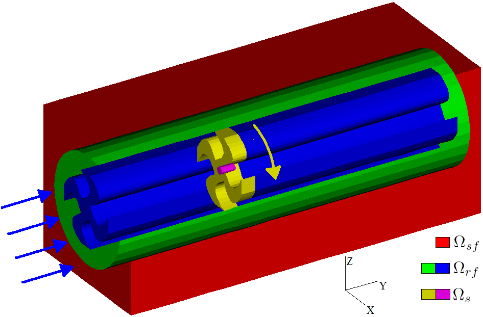
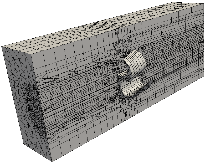
Figure 4: The 3D self defined elastic rotor: $\Omega=\Omega_{s}+\Omega_{f}$ and $\Omega_{f}=\Omega_{sf}+\Omega_{rf}$, and the mesh of half domain, where the interfaces $\Gamma_{rs}=\partial\Omega_{rf}\cap\partial\Omega_{sf}$ and $\Gamma=\partial\Omega_{rf}\cap\partial\Omega_{s}$.

As illustrated by Fig. 4, we define a cylindrical fluid subdomain $\Omega_{rf}\subset\Omega_{f}$ to embrace the elastic rotor $\Omega_{s}$ and rotate together on the same axis of rotation. Let $\Omega_{sf}:=\Omega_{f}\backslash\Omega_{rf}$ denote the rest of the fluid domain that is stationary. Moreover, on the interface between $\Omega_{sf}$ and $\Omega_{rf}$, $\Gamma_{sf}$, and the interface between $\Omega_{rf}$ and $\Omega_{s}$, $\Gamma$, we apply the Master-Slave relations to the pairs of grid points along with a certain triangulation pattern. Such triangulation pattern on the interface $\Gamma_{rs}$ is defined in a specific manner such that it is easy to search and reconnect each pair of the grid point when the slave point on one side ($\partial\Omega_{rf}$) rotates away from its master point on the other side ($\partial\Omega_{sf}$). For instance, since we need to choose an axisymmetric domain as the rotational fluid domain $\Omega_{rf}$, the cross section that is perpendicular to the central axis of $\Omega_{rf}$ is always a disk, on which the grid pattern can be triangulated as shown in Fig. 5 in order to easily search the paired grid points on $\Gamma_{rs}$. We basically use the approach shown in Fig. 3 to re-match each point pair on $\Gamma_{rs}$ when they are away from each other. Therefore, the entire fluid mesh retains the conformity.

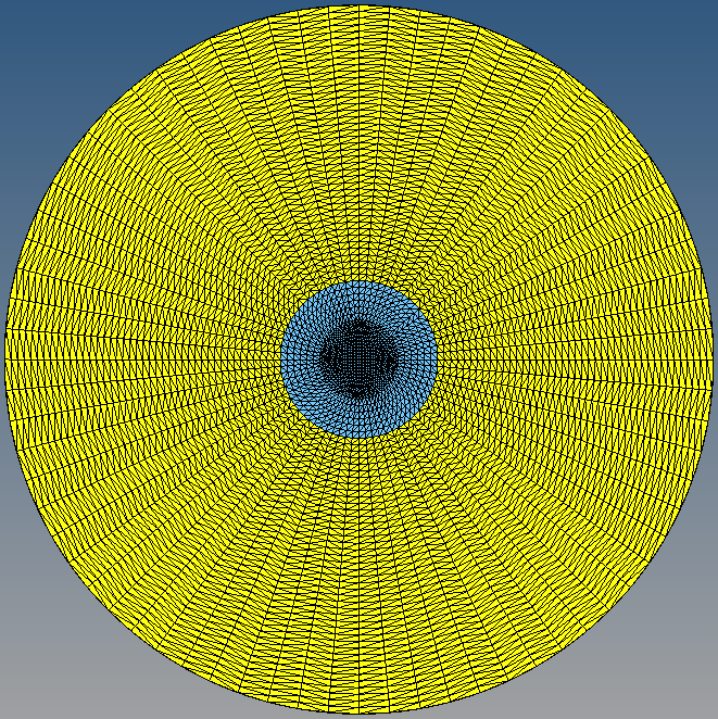
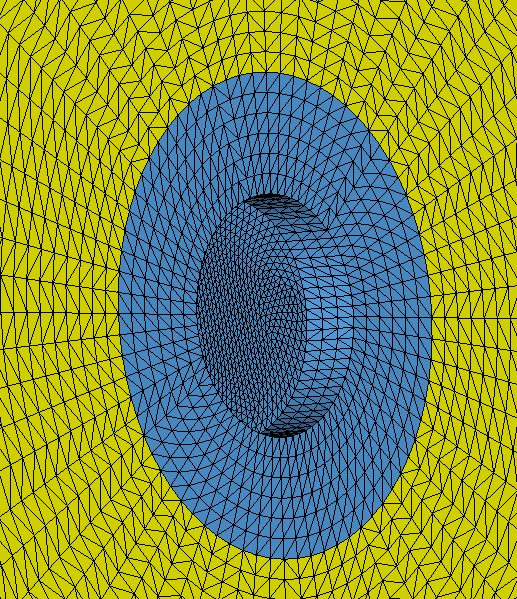
Figure 5: The triangulation pattern on the interface of the rotational fluid domain $\Omega_{rf}$ and the stationary fluid domain $\Omega_{sf}$.

Thereafter, by means of $P_{1}$-$P_{1}$ mixed element with pressure stabilization to discretize momentum and mass equations, linear finite element to discretize ALE equation, and Algorithm 1, we obtain the following numerical results with the time step size $\Delta t=0.01$s and the mesh size $h<0.02$m, as shown in Figs. 6-7.

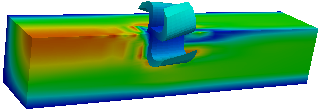
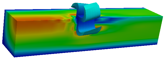
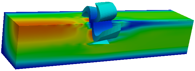
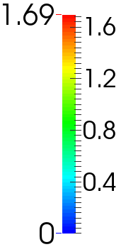
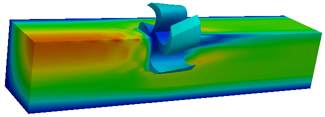
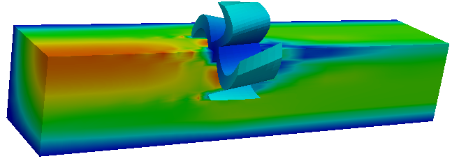
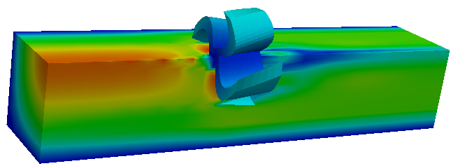
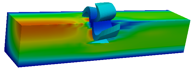
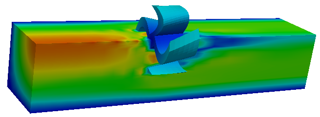
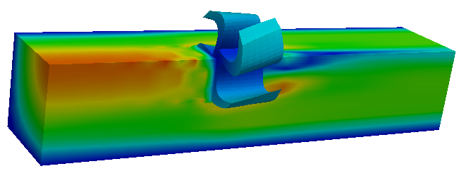
(a) Time=2s (b) Time=4s (c) Time=6s (d) Time=8s (e) Time=10s (f) Time=12s (g) Time=14s (h) Time=16s (i) Time=18s

Figure 6: A self-defined elastic rotor: the evolution of magnitude of velocity with time in 1/4 fluid domain.

Fig. 6 illustrates the evolution of the magnitude of velocity field with time marching in a quarter part of the fluid domain along the flow direction, while the incoming fluid keeps flowing in the inlet with the prescribed maximum velocity magnitude, 1.5 m/s, and gets detoured by the elastic rotor which preserves spinning around its axis of rotation in the plane that is perpendicular to the flow direction with the prescribed angular velocity, 1 rad/s. With these given steady velocities, we can observe that the entire fluid field basically attains a relatively steady state after 2s, the fluid flow is significantly disturbed near the spinning turbine, such disturbance dies away along with the increasing distance from the turbine. The magnitude of velocity field forms a nearly vacuum region behind the turbine in which the velocity magnitude is much smaller than elsewhere due to the lower pressure there, and a portion of this region that is nearest to the turbine is twisted by the spin, periodically. Fig. 7 shows the streamline field and velocity vector field at 19s, respectively, further illustrating the disturbance status of the fluid right after it flows over the spinning turbine, where, the streamline is twisted away from the mainstream near the turbine due to its spin, then merges back again when the fluid is relatively far away from the turbine, and continue to flow straight to the outlet.

Note that the magnitude of Reynolds number that we adopt in this example is just 100 or so, truly resulting in a laminar flow. Since we only focus on the methodology study of simulating the dynamical interaction between an elastic rotor and the fluid, the fluids with a large Reynolds number or even turbulence flow are not our concern in this paper. In the future, we will consider a turbulence model for fluids with a large Reynolds number, but the ALE approach and the monolithic algorithm developed in this paper are still valid for the simulation of the interaction between the turbulent flow and a hydro-turbine.

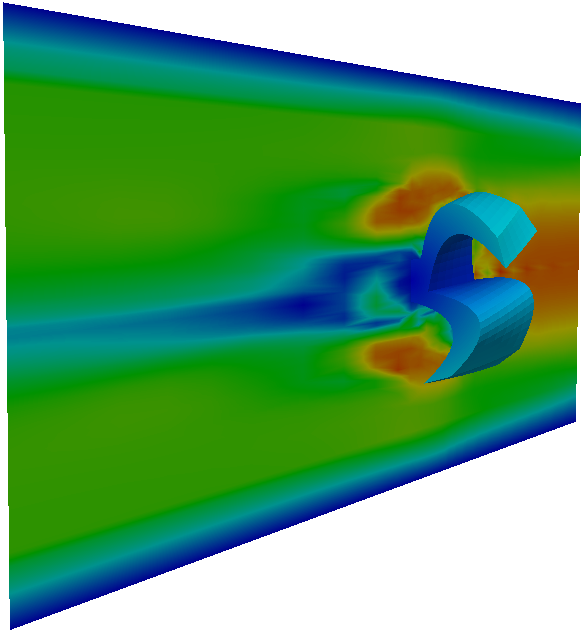
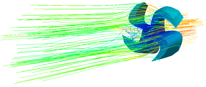
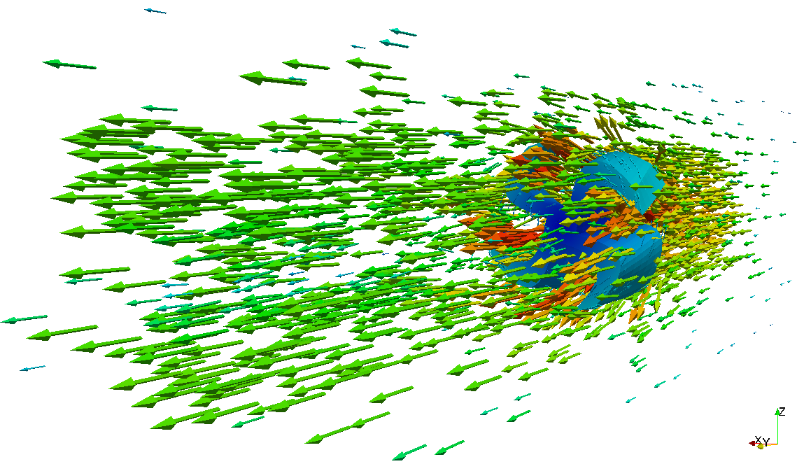
(a) Magnitude of velocity field (b) Streamline field (c) Velocity field

Figure 7: A self-defined elastic rotor: magnitude of velocity field on the central cross section along flow direction (left); streamline (middle) and velocity (right) fields at 19s.

It is not easy to observe the deformation of the elastic rotor since its stiffness is measured by a relatively large Young’s modulus (2.5 MPa) in this example. To show the deformation of a spinning rotor due to the fluid impact, we need to look at some extreme circumstances, e.g., a flexible and/or a thinner rotor with smaller Young’s modulus, in order to observe a dramatically large deformation occurring on the hydro-turbine blades while rotating. Fig. 8 illustrates the desired numerical results, where the self defined flexible and thinner blades with a relatively smaller Young’s modulus deform while rotate, dramatically.

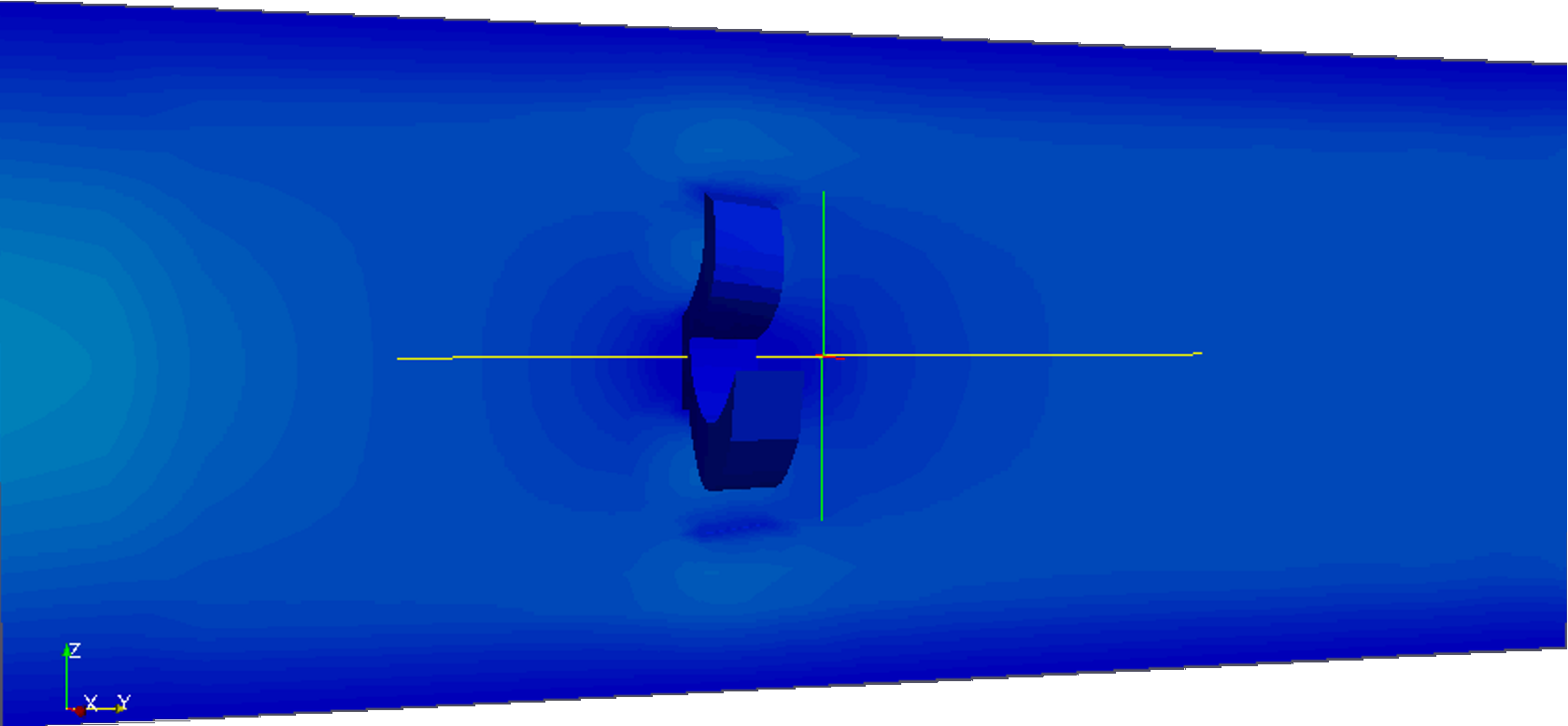
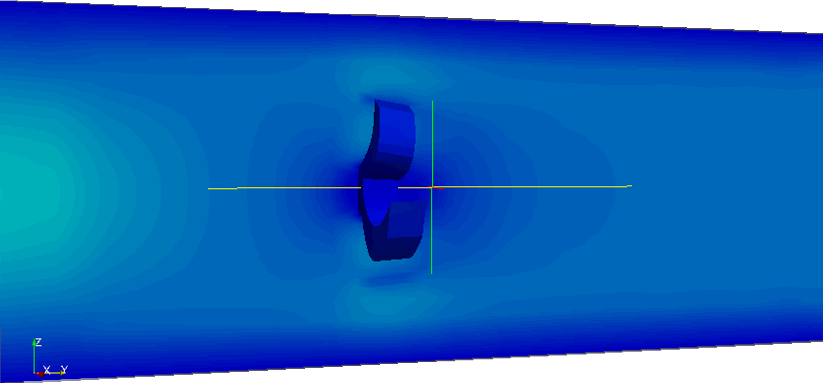
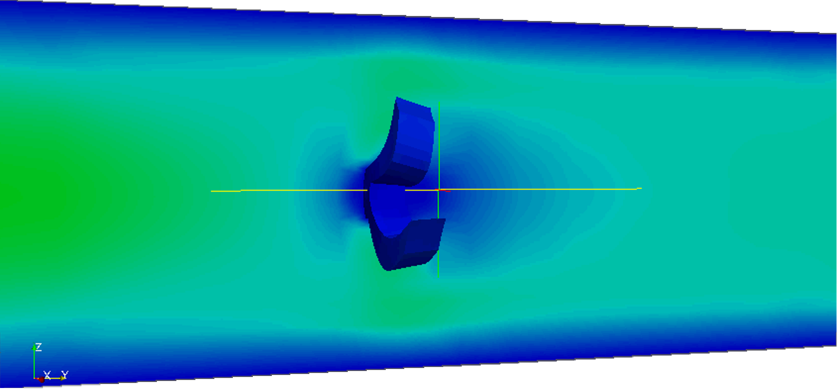
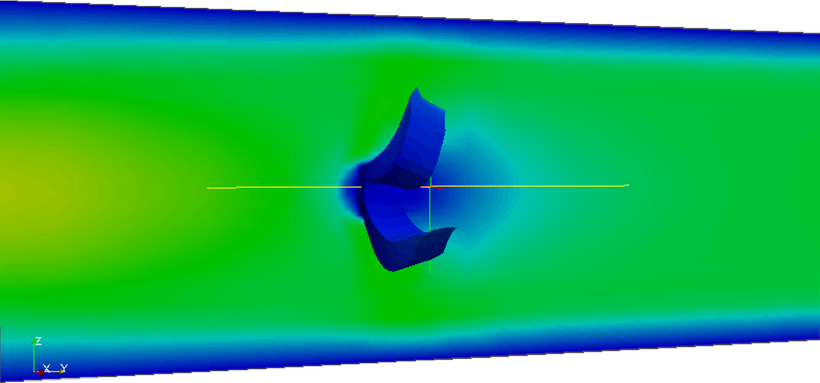
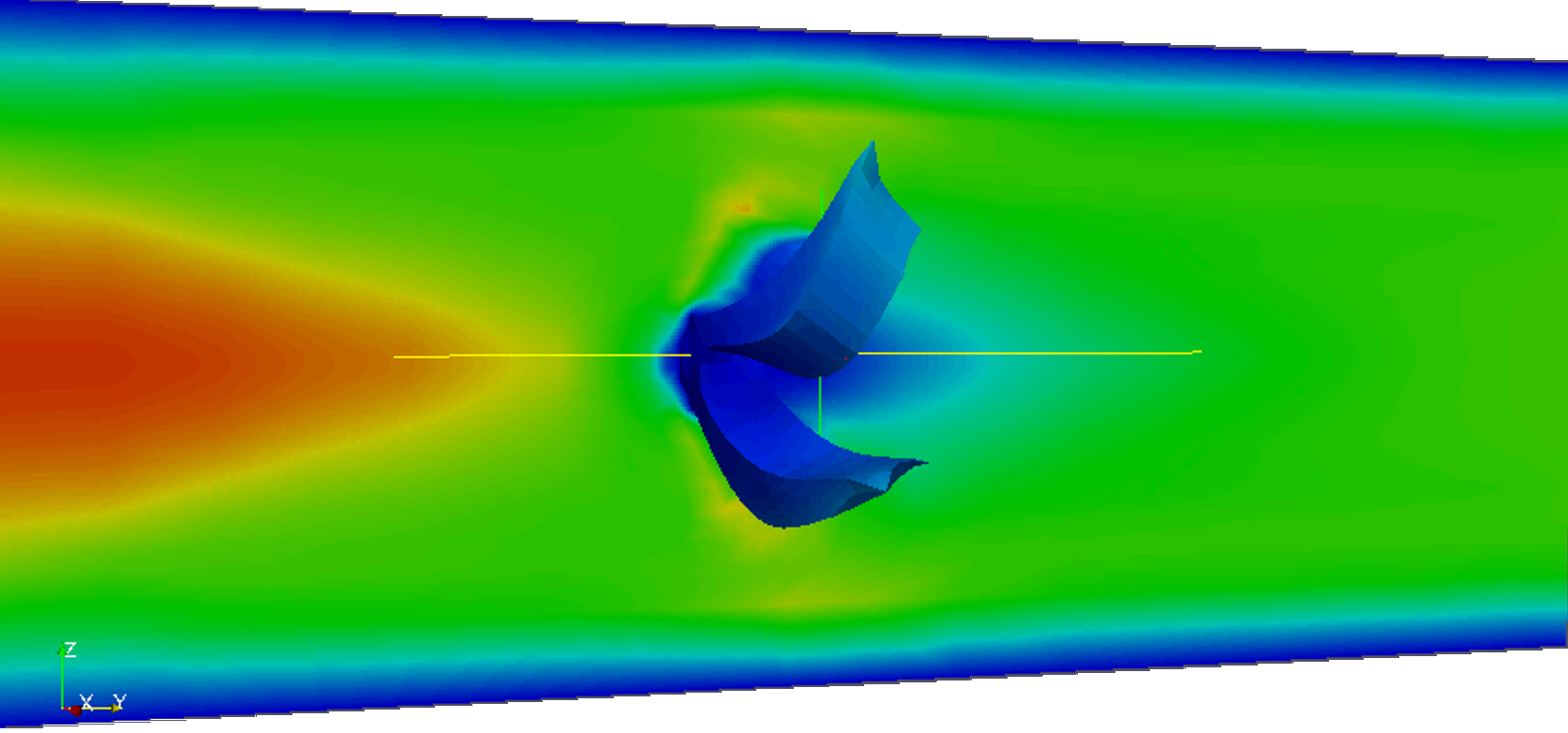
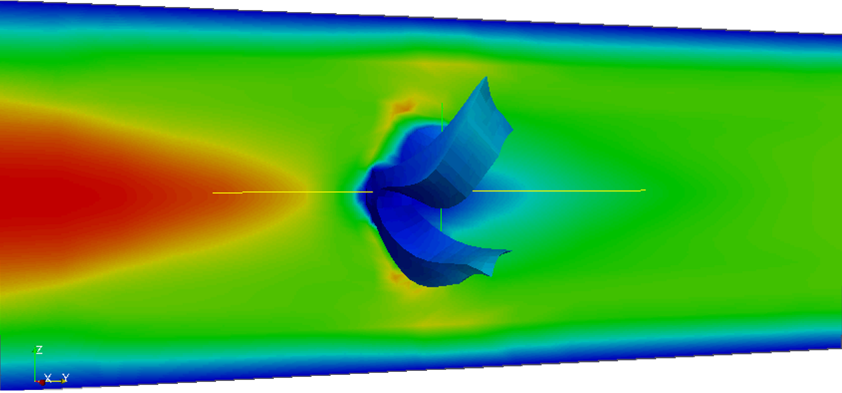
(a) Time=0.06s (b) Time=0.12s (c) Time=0.18s (d) Time=0.24s (e) Time=0.3s (f) Time=0.36s

Figure 8: A more flexible and thinner elastic rotor which deforms while rotates: the evolution of magnitude of velocity field with time on the central cross section along flow direction.

Now we conduct a consistency check for the developed structure model. We carry out a series of numerical computations for the fluid-turbine interaction with respect to an increasing Young’s modulus of the turbine, for instance, from $E=2.5\times 10^{4}$ Pa all the way up to $E=2.5\times 10^{9}$ Pa, which means the turbine tends to be stiffer and stiffer toward a rigid body. Because a rigid body does not deform, one shall expect that the deformation displacement in any place of the turbine approaches to zero along with an increasing Young’s modulus. To that end, we just need to check the displacement component in flow direction since there is not any the component of rotational displacement existing in that direction. By the configuration, we set the turbine to spin only in the plane which is perpendicular to the flow direction. In addition, since the blade tip is the thinnest part in the turbine, it bears relatively the largest deformation during the interaction with the fluid. Thus, by checking the variation tendency of the blade tip displacement in flow direction along with the increasing Young’s modulus, we are able to validate our developed structure model in the sense of an asymptotic stiffness. Fig. 9 shows a semi logarithmic plot of the variation of blade tip displacement in flow direction along with time and the increasing Young’s modulus, where the displacement component is logarithmically scaled in order to distinctly illustrate that the blade tip displacement approaches to zero while the Young’s modulus becomes much larger at any instantaneous time, demonstrating that the developed structure model is consistently correct and the developed numerical method is convergent with respect to a crucial physical parameter of structure that may vary, asymptotically.

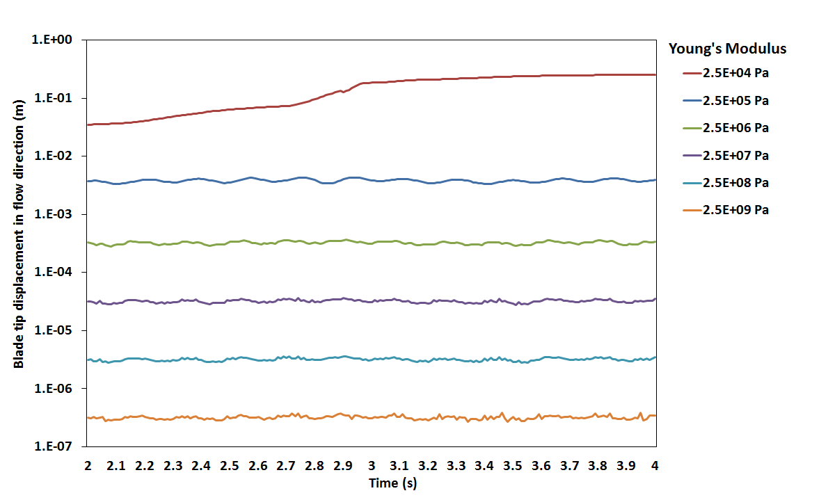
Figure 9: The variation tendency of blade tip displacement in flow direction at the central line of the rotor thickness along with the increasing Young’s modulus and time, where the ordinate is scaled logarithmically.

Next, we apply our validated monolithic ALE method to a practical fluid-structure interaction problem involving a realistic three-dimensional hydro-turbine which is still under construction for a new hydro plant. As illustrated in Figs. 10-11, a realistic turbine bears five blades curved in three-dimensional fashion and is immersed in the fluid domain with a shape of circular truncated cone. Thus, we take advantage of the shape of fluid flow channel and make the entire fluid domain as rotational, thus no stationary fluid domain exists in this example. By doing that way we simply solve the ALE mapping equation in the entire fluid domain to obtain the entire fluid mesh with zero boundary condition on the outer boundary of $\hat{\Omega}_{f}$. Under the same prescribed incoming velocity and angular velocity as given for the previous self-defined rotor, we obtain the similar illustrations for the numerical results shown in Figs. 12-13. Fig. 12 displays the development of velocity magnitude with time marching in a quarter part of fluid domain along the flow direction, and Fig. 13 shows the velocity field in the streamline as well as the vector version.

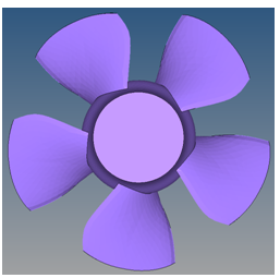
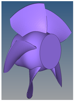
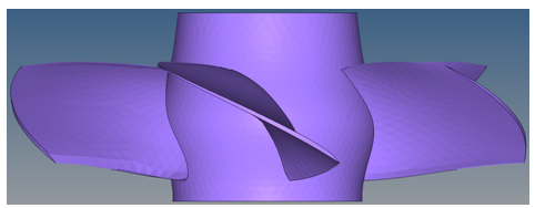
Figure 10: A realistic 3D turbine.

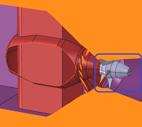
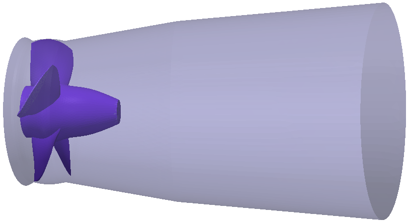
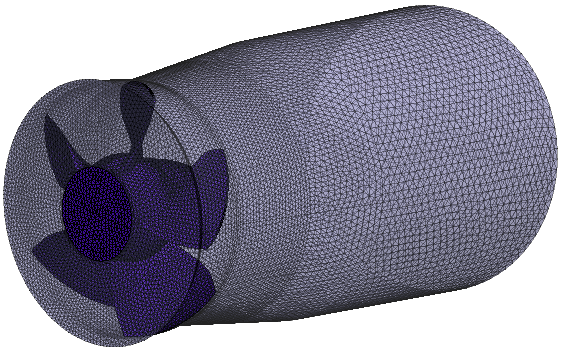
Figure 11: The realistic turbine immersed in the fluid domain with the shape of a circular truncated cone: $\Omega=\Omega_{s}+\Omega_{f}$ and $\Omega_{f}=\Omega_{rf}$, no stationary fluid domain $\Omega_{sf}$, and the only interface is $\Gamma=\partial\Omega_{f}\cap\partial\Omega_{s}$.

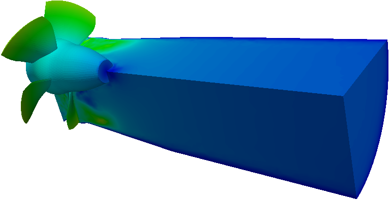
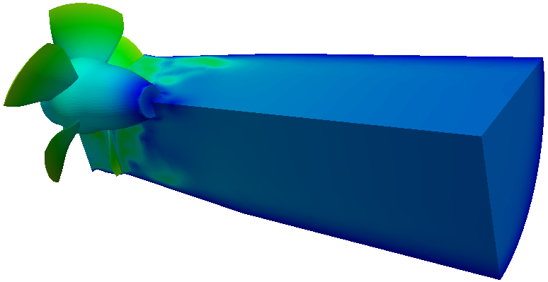
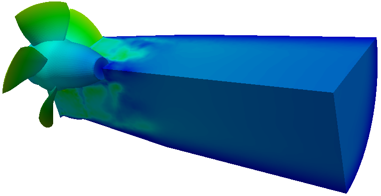
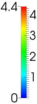
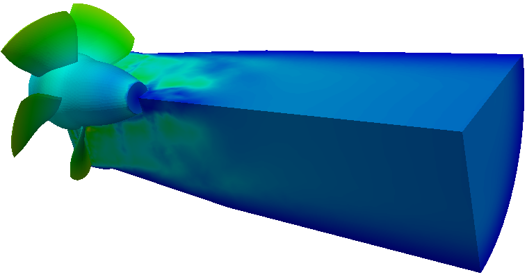
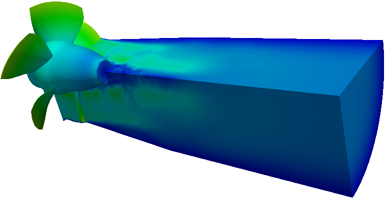
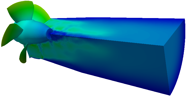
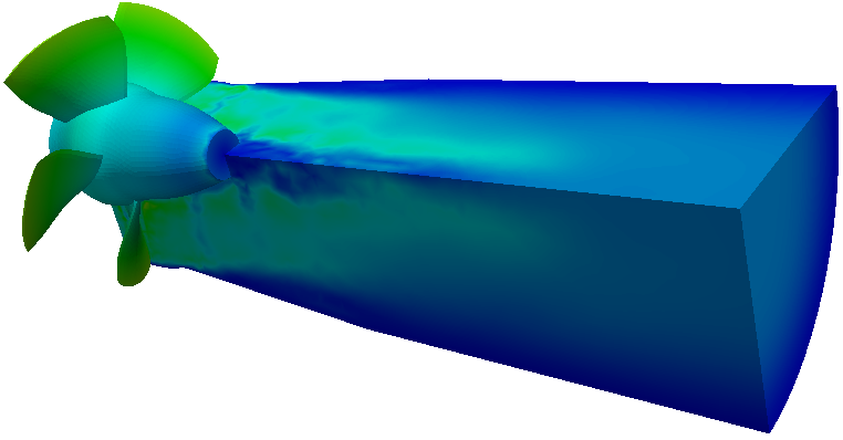
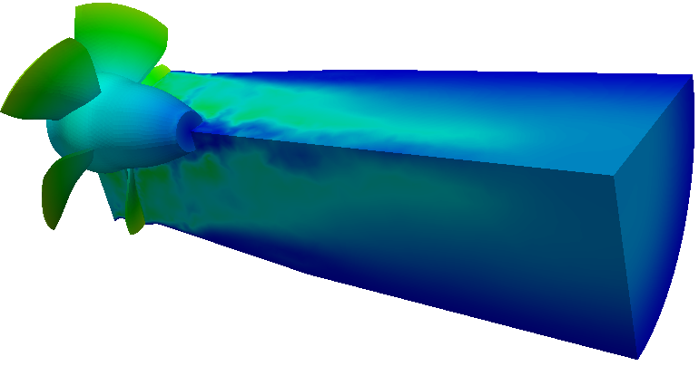
(a) Time=1.6s (b) Time=3.15s (c) Time=4.75s (d) Time=6.35s (e) Time=7.9s (f) Time=9.5s (g) Time=11.05s (h) Time=12.65s (i) Time=14.25s

Figure 12: A realistic elastic rotor: the evolution of magnitude of velocity with time in 1/4 fluid domain.

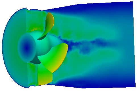
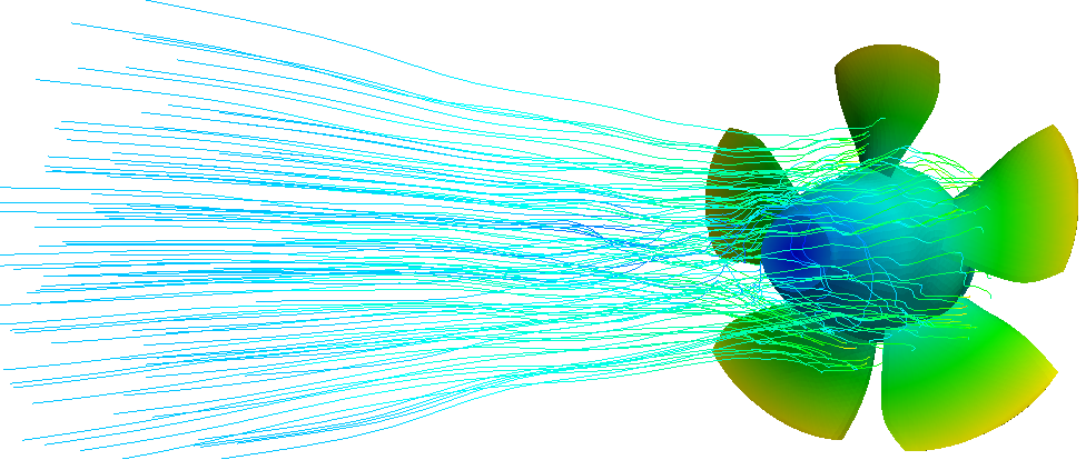
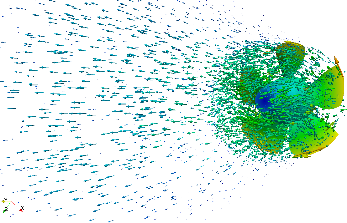
(a) Magnitude of velocity field (b) Streamline field (c) Velocity field

Figure 13: A realistic elastic rotor: magnitude of velocity field on the central cross section along flow direction (left); streamline (middle) and velocity (right) fields at 14.25s.

Remark 5.

In some senses, our current model and numerical method also work for the passive rotational case, i.e., for which there is not a prescribed angular velocity on the axis of rotation. In this case, we do not know the structure velocity on the cylindrical axis of rotation $\Gamma_{in}$. In order to make the initially static turbine spinning up while the fluid flow starts to impact, we can shrink the cylindrical axis of rotation as a point axis (or a line axis in 3D) on its barycenter, and fix the structure displacement and then velocity as zero on the point/line axis, thus the turbine is not be carried away by the fluid flow but likely rotates about the point/line axis if the external fluid force is acted on the turbine. This configuration is inaccurate in the mathematical point of view but numerically works to some extent, with which we are still able to apply our developed model and numerical methods to the FSI problem involving with a passively rotational hydro-turbine, and observe that the elastic turbine starts to spin up from its initially static position, and accelerates its rotation until reaching a steady rotational status, i.e., the fluid impact force acting on the turbine attains a balance with the resistance force arising from the fluid itself due to the viscosity, if there is not any other external torque being exerted on the turbine.

However, we do not intend to illustrate the numerical results of passive rotational case in this paper since the inaccurate configuration of (d-2)-dimensional axis does not make fully mathematical sense, and additionally, might also introduce extra stress concentration effect on such (d-2)-dimensional axis under a large external load. Recently we develop a novel and more accurate numerical method for the passive rotational case, which will be the subject of a forthcoming paper.

10 Conclusions

We build an Eulerian-Lagrangian model for fluid-structure interaction problem involving with an elastic rotor based on the arbitrary Lagrangian Eulerian (ALE) approach. Using velocity as the principle unknown in structure equation, we are able to deal with the no-slip condition on the interface of fluid and structure more flexibly with the technique of Master-Slave Relations. In addition, with the variational formulation and mixed finite element method, the interface conditions are automatically enforced. Our proposed novel ALE method can flexibly generate a rotational and deformable fluid mesh according to the boundary conditions arising from the ambient elastic rotor and the stationary fluid. The linear system resulting from linearization and discretization is proved to be well-posed. By means of the developed monolithic algorithm involving the relaxed fixed-point iteration, a series of satisfactory numerical results are illustrated and validated for the elastic hydro-turbine that is actively spinning around its axis of rotation and interacting with the fluid, demonstrating that our model and numerical techniques are effective to explore the interactional mechanism between the fluid and an elastic rotor. As a part of the future work, we will continue to develop the numerical method for the case of passive rotation that is more suitable for the hydro-turbine, and further, study the FSI problem in which the turbulence flow is involved.

References

- [1] S. Badia, A. Quaini, and A. Quarteroni. Modular vs. non-modular preconditioners for fluid–structure systems with large added-mass effect. Comput. Methods Appl. Mech. Eng., 197(49-50):4216–4232, 2008.
- [2] S. Badia, A. Quaini, and A. Quarteroni. Splitting methods based on algebraic factorization for fluid-structure interaction. SIAM J. Sci. Comput., 30(4):1778–1805, 2008.
- [3] A. Barker and X.-C. Cai. NKS for fully coupled fluid-structure interaction with application. Domain Decomposition Methods in Science and Engineering XVIII, pages 275–282, 2009.
- [4] A. T. Barker and X.-C. Cai. Scalable parallel methods for monolithic coupling in fluid–structure interaction with application to blood flow modeling. J. Comput. Phys., 229(3):642–659, 2010.
- [5] A. T. Barker and X.-C. Cai. Two-level Newton and hybrid Schwarz preconditioners for fluid-structure interaction. SIAM J. Sci. Comput., 32(4):2395–2417, 2010.
- [6] Y. Bazilevs and M. Hsu. 3D simulation of wind turbine rotors at full scale. Part I: geometry modeling and aerodynamics. Int. J. Numer. Meth. Fluids, 65:207–235, 2011.
- [7] Y. Bazilevs, M. Hsu, J. Kiendl, R. Wüchner, and K. Bletzinger. 3D simulation of wind turbine rotors at full scale . Part II : Fluid-structure interaction modeling with composite blades. Int. J. Numer. Meth. Fluids, 65:236–253, 2011.
- [8] Y. Bazilevs, M. Hsu, and M. Scott. Isogeometric fluid-structure interaction analysis with emphasis on non-matching discretizations, and with application to wind turbines. Comput. Methods Appl. Mech. Eng., 249-252:28–41, 2012.
- [9] Y. Bazilevs, M. Hsu, K. Takizawa, and T. Tezduyar. ALE-VMS and ST-VMS methods for computer modeling of wind-turbine rotor aerodynamics and fluid-structure interaction. Math. Models Methods Appl. Sci., 22(2):1230002, 2012.
- [10] Y. Bazilevs, K. Takizawa, and T. E. Tezduyar. Computational fluid-structure Interactions: Methods and Applications. Wiley, 2013.
- [11] M. Behr and T. Tezduyar. The shear-slip mesh update method. Comput. Methods Appl. Mech. Eng., 174:261–274, 1999.
- [12] M. Behr and T. Tezduyar. Shear-slip mesh update in 3D computation of complex flow problems with rotating mechanical components. Comput. Methods Appl. Mech. Eng., 190:3189–3200, 2001.
- [13] T. Belytschko and J. Kennedy. Computer models for subassembly simulation. J. Nucl. Eng. Design, 49:17–38, 1978.
- [14] T. Belytschko, J. Kennedy, and D. Schoeberle. Quasi-Eulerian finite element formulation for fluid-structure interaction. J. Press. Vess-T ASME, 102:62–69, 1980.
- [15] F. Brezzi and J. Pitkaranta. On the stabilization of finite element approximations of Stokes problem. In W. Hackbusch, editor, Efficient Solutions of Elliptic Systems, volume 10 of Notes on Numerical Fluid Mechanics, pages 11–19. Vieweg-Verlag, 1984.
- [16] X.-C. Cai. Two-level Newton and hybrid Schwarz preconditioners for fluid-structure interaction. SIAM J. Sci. Comput., 32(4):2395–2417, 2010.
- [17] S. Capdevielle. Modeling fluid-rigid body interaction using the Arbitrary Lagrangian Eulerian Method. Masters Abstracts International, 51, 2012.
- [18] B. Desjardins. On weak solutions for fluidrigid structure interaction: Compressible and incompressible models. Commun. Part. Diff. Eq., 25:263–285, 2000.
- [19] J. Donea, S. Giuliani, and J. Halleux. An arbitrary Lagrangian-Eulerian finite element method for transient dynamic fluid-structure interactions. Comput. Meth. Appl. Mech. Eng., 33(1):689–723, 1982.
- [20] Q. Du, M. Gunzburger, L. Hou, and J. Lee. Analysis of a linear fluid-structure interaction problem. Disc. Conti. Dyn. Sys.-A, 9:633–650, 2003.
- [21] C. Felippa and B. Haugen. A unified formulation of small-strain corotational finite elements: I. Theory. Comput. Methods Appl. Mech. Engrg., 194:2285–2335, 2005.
- [22] M. W. Gee, U. Küttler, and W. A. Wall. Truly monolithic algebraic multigrid for fluid-structure interaction. Int. J. Numer. Methods Eng., 85(8):987–1016, 2011.
- [23] V. Girault and P. Raviart. Finite element methods for Navier-Stokes equations: Theory and algorithms. Springer Ser. Comput. Math, 5, 1986.
- [24] M. Heil. An efficient solver for the fully coupled solution of large-displacement fluid-structure interaction problems. Comput. Methods Appl. Mech. Engrg., 193(1-2):1–23, 2004.
- [25] C. Hirth, A. Amsden, and J. Cook. An arbitrary Lagrangian-Eulerian computing method for all flow speeds. Journal of Computational Physics, 14:227–253, 1974.
- [26] G. Hou, J. Wang, and A. Layton. Numerical methods for fluid-structure interaction - a review. Commun. Comput. Phys., 12:337–377, 2012.
- [27] M. Hsu and Y. Bazilevs. Fluid-structure interaction modeling of wind turbines: simulating the full machine. Comput. Mech., 50:821–833, 2012.
- [28] H. Hu. Direct simulation of flows of solid-liquid mixtures. Int. J. Multiphase Flow, 22:335–352, 1996.
- [29] A. Huerta and W. Liu. Viscous flow structure interaction. Trans. ASME J. Pressure Vessel Technol., 110:15–21, 1988.
- [30] T. Hughes, W. Liu, and T. Zimmermann. Lagrangian-Eulerian finite element formulation for incompressible viscous flows. Comput. Methods Appl. Mech. Eng., 29:329–349, 1981.
- [31] T. J. R. Hughes, L. P. Franca, and M. Balestra. A new finite element formulation for computational fluid dynamics: V. circumventing the Babuska-Brezzi condition: A stable Petrov-Galerkin formulation of the Stokes problem accommodating equal-order interpolations. Comput. Meth. Appl. Mech. Eng., 59:85–99, 1986.
- [32] S. Idelsohn, P. Del, R. Rossi, and E. O. nate. Fluid-structure interaction problems with strong added-mass effect. Int. J. Numer. Methods Eng., 80:1261–1294, 2009.
- [33] A. Johnson and T. Tezduyar. 3D simulation of fluid-particle interactions with the number of particles reaching 100. Comput. Methods Appl. Mech. Eng., 145:301–321, 1997.
- [34] C. Johnson, U. Navert, and J. Pitkaranta. Finite element methods for linear hyperbolic problems. Comput. Meth. Appl. Mech. Eng., 45:285–312, 1984.
- [35] A. Masud. A space-time finite element method for fluid-structure interaction. PhD thesis, Stanford University, 1993.
- [36] C. Nitikitpaiboon and K. Bathe. An arbitrary Lagrangian-Eulerian velocity potential formulation for fluid-structure interaction. Comput. Struct., 47:871–891, 1993.
- [37] F. Nobile. Numerical Approximation of Fluid-Structure Interaction Problems with Application of Haemodynamics. PhD thesis, Ecole Polytechnique Federale de Lausanne, Switzerland, 2001.
- [38] T. Richter. A fully Eulerian formulation for fluid-structure interaction problems. J. Comput. Phys., 233:227–240, 2013.
- [39] T. Richter and T. Wick. Finite elements for fluid-structure interaction in ALE and fully Eulerian coordinates. Comput. Methods Appl. Mech. Engrg., 199:2633–2642, 2010.
- [40] P. B. Ryzhakov, R. Rossi, S. R. Idelsohn, and E. Oate. A monolithic Lagrangian approach for fluid-structure interaction problems. Comput. Mech., 46:883–899, 2010.
- [41] J. Sarrate, A. Huerta, and J. Donea. Arbitrary Lagrangian-Eulerian formulation for fluid-rigid body interaction. Comput. Methods Appl. Mech. Engrg, 190:3171–3188, 2001.
- [42] M. Souli and D. J. Benson, editors. Arbitrary Lagrangian Eulerian and fluid-structure Interaction: Numerical Simulation. Wiley-ISTE, 2010.
- [43] K. Sugiyama, S. Ii, S. Takeuchi, S. Takagi, and Y. Matsumoto. A full Eulerian finite difference approach for solving fluid-structure coupling problems. J. Comput. Phys., 230:596–627, 2011.
- [44] C. Taylor, T. Hughes, and C. Zarins. Finite element modeling of blood flow in arteries. Comput. Methods Appl. Mech. Eng., 158:155–196, 1998.
- [45] T. E. Tezduyar. Stabilized finite element formulations for incompressible flow computations. Adv. Appl. Mech., 28:1–44, 1992.
- [46] S. Turek and J. Hron. Numerical Simulation and Benchmarking of a Monolithic Multigrid Solver for Fluid-Structure Interaction Problems with Application to Hemodynamics. Fluid Structure Interaction II:Modelling, Simulation, Optimization, 73:193, 2010.
- [47] D. Veubeke and B. Fraeijs. The dynamics of flexible bodies. Int. J. Eng Sci., 14(10):895–913, 1976.
- [48] Y. Wu and X.-C. Cai. A fully implicit domain decomposition based ale framework for three-dimensional fluid–structure interaction with application in blood flow computation. J. Comput. Phys., 258:524–537, 2014.
- [49] J. Xu and K. Yang. Well-posedness and robust preconditioners for discretized fluid–structure interaction systems. Computer Methods in Applied Mechanics and Engineering, 292:69–91, 2015. Special Issue on Advances in Simulations of Subsurface Flow and Transport (Honoring Professor Mary F. Wheeler).
- [50] L. Zhang, Y. Guo, and W. Wang. Large eddy simulation of turbulent flow in a true 3D francis hydroturbine passage with dynamical fluid-structure interaction. Int. J. Numer. Meth. Fluids, 54:517–541, 2007.
- [51] L. Zhang, Y. Guo, and W. Wang. Fem simulation of turbulent flow in a turbine blade passage with dynamical fluid-structure interaction. Int. J. Numer. Meth. Fluids, 61:1299–1330, 2009.
- [52] L. Zhang, Y. Guo, and H. Zhang. Fully coupled flow-induced vibration of structures under small deformation with gmres method. Appl. Math. Mech., 31:87–96, 2010.