Hemispheric Differences in the Response of the Upper Atmosphere to the August 2011 Geomagnetic Storm: A Simulation Study

Abstract

Using a three-dimensional nonhydrostatic general circulation model, we investigate the response of the thermosphere-ionosphere system to the 5–6 August 2011 major geomagnetic storm. The model is driven by measured storm-time input data of the Interplanetary Magnetic Field (IMF), solar activity, and auroral activity. Simulations for quiet steady conditions over the same period are performed as well in order to assess the response of the neutral and plasma parameters to the storm. During the storm, the high-latitude mean ion flows are enhanced by up to 150–180%. Largest ion flows are found in the main phase of the storm. Overall, the global mean neutral temperature increases by up to 15%, while the maximum thermal response is higher in the winter Southern Hemisphere at high-latitudes than the summer Northern Hemisphere: 40% vs. 20% increase in high-latitude mean temperature, respectively. The global mean Joule heating increases by more than a factor of three. There are distinct hemispheric differences in the magnitude and morphology of the horizontal ion flows and thermospheric flows during the different phases of the storm. The largest hemispheric difference in the thermospheric circulation is found during the main and recovery phases of the storm, demonstrating appreciable geographical variations.The advective forcing is found to contribute to the modeled hemispheric differences.

1 Introduction

The thermosphere ($\sim 90-500$ km) is the upper part of the neutral atmosphere that coexists with and is dynamically and chemically coupled to the ionosphere via electrodynamical and wave processes. The thermosphere is influenced by lower atmospheric internal waves (Altadill et al., 2004; Abdu et al., 2006; Pancheva et al., 2009; Yiğit and Medvedev, 2010, 2015) and exhibits large solar and geomagnetic variations (Emery et al., 1999; Immel et al., 2001; Balan et al., 2011). Owing to the simultaneous interplay of upward wave propagation, space weather effects, and internal processes, the upper atmosphere has substantial spatiotemporal variability (Innis and Conde, 2002; Matsuo et al., 2003; Bristow, 2008; Anderson et al., 2011; Kil et al., 2011; Pancheva and Mukhtarov, 2011; Yiğit et al., 2012a).

Geomagnetic storms are a central aspect of “space weather” that can have a great impact on, for example, airline crew and passengers, telecommunication systems, electric power grids, and satellite navigation. Therefore space weather is considered a subject of natural hazard. The origin of space weather is the high-energy plasma ejection by the Sun into the interplanetary space. Sudden high-density plasma ejection processes can be detected by the NASA-European Space Agency (ESA) Solar and Heliospheric Observatory (SOHO) spacecraft. An extreme form of plasma ejection is the coronal mass ejection (CME) that is a large eruption of magnetic field and plasma from the outer atmosphere of the Sun. A CME directed toward Earth with a typical speed of 1000 km s^-1 would take about 40 hours to reach Earth and can produce major geomagnetic storms. Improved predictions though are necessary to be able to take the necessary precautions in cases of extreme storm events However, space weather predictions are relatively limited. Even in the case of terrestrial lower atmospheric weather, predictions can be done only to a certain extent, despite the advances in modern technology that allows a detailed monitoring.

In broader terms, space weather is understood as the effects of the Sun-magnetosphere system on Earth’s atmosphere-ionosphere system. What is then a geomagnetic storm? Gonzalez et al. (1994) describe a geomagnetic storm as a period during which sufficiently intense long-lasting interplanetary convection electric fields are present and the magnetosphere-ionosphere system is substantially energized. That is, an interplanetary electric field causes convection in the magnetosphere-ionosphere system.

Geomagnetic storms can have great impact on Earth’s environment. Storm-induced thermospheric mass density enhancement can affect satellite orbital lifetimes and expectancy (Prölss, 2011) and can make Global Position System signals undergo rapid fluctuations in amplitude and phase. While terrestrial “meteorological storms” (e.g., hurricanes, thunderstorms) have direct impact on Earth’s lower atmosphere, the influences of “space weather storms” on Earth’s atmosphere are indirect, primarily via the changes in the magnetosphere and the subsequent downward coupling to the atmosphere-ionosphere system therefrom. The intensity of geomagnetic storms are extremely variable (Mannucci et al., 2005).

Historically, magnetic storms were discussed theoretically before the advent of global satellite technology (e.g., Martyn, 1951). Later, computer models have been developed based on theoretical equations in order to predict the response of the upper atmosphere to storms. Earlier numerical modeling efforts have provided valuable insight into high-latitude ionospheric convection and the effects of geomagnetic storms. With a longitudinally invariant hydrostatic numerical model that assumes a coincident geomagnetic field with the Earth’s rotational axis, Richmond and Matsushita (1975) demonstrated equatorward propagating large-scale gravity waves (GWs) during a substorm. Equatorward propagating large-scale GWs can transfer energy and momentum from the high-latitudes to low-latitudes. General circulation modeling efforts by Roble et al. (1982) excluding the effects of particle precipitation showed that ionospheric plasma convection constitutes a substantial amount of momentum and energy source at high-latitudes.

Various aspects of geomagnetic storms have been investigated by three-dimensional nonlinear hydrostatic upper atmosphere models (e.g., Fuller-Rowell and Rees, 1981; Emery et al., 1999; Zaka et al., 2010; Burns et al., 2012; Lu et al., 2013) as well as by observations (e.g., Oliver et al., 1988; Anderson et al., 1998; Balan et al., 2011, 2012; Kil et al., 2011; Ma et al., 2012). Today, advances in satellite technologies enable continuous monitoring and characterization of the geospace environment and computer models are used to diagnose the effects of solar and geomagnetic variations on Earth’s upper atmosphere.

Recently, a series of geomagnetic storm events occurred between August–October 2011 that motivated researchers to better characterize these storms (e.g., Earle et al., 2013; Gong et al., 2013; Haaser et al., 2013; Blanch et al., 2013; Huang et al., 2014). While increased amount of observations of the geospace during storms help researchers characterize these storms in more detail, application of coupled nonlinear global models can provide a framework to determine possible storm effects on the upper atmosphere. Satellite observations can be used to drive global atmosphere-ionosphere models that require boundary conditions with measured magnetospheric variations in order to simulate the consequences of storms on the upper atmosphere, i.e., the thermosphere-ionosphere.

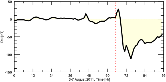
Figure 1: Variations of the Disturbed Storm Time index ($Dst$) retrieved from the World Data Center for Geomagnetism, Kyoto, in nT from 3 to 7 August 2011 (96-hour period). The horizontal and vertical dotted red lines denote the 0 nT level and the beginning of the disturbed period, respectively.

The goal of this paper is to apply general circulation modeling techniques to investigate the storm-time global changes in the upper atmosphere in ways that have not done before, to address the previously challenging problem of hemispheric differences and to understand the related dynamical mechanisms. The unique aspects of the August 2011 geomagnetic storm offer an ideal case to extend previous studies, and having done so we can offer new physical insights in geomagnetic storm forcing and the resultant effects in the upper atmosphere. Specifically, we use the Global Ionosphere Thermosphere Model ((GITM), Ridley et al., 2006), which is a three-dimensional nonlinear nonhydrostatic general circulation model (GCM) that self-consistently couples the thermosphere and ionosphere. Observations of the August 2011 geomagnetic storm from NASA’s Advanced Composition Explorer (ACE) satellite will be used as model input in order to perform simulations under realistic storm conditions. The main focus of the paper is the dynamical response of the upper atmosphere to the storm.

The structure of the paper is as follows: The next section describes the observations of the August 2011 geomagnetic storm; sections 3–4 introduce the GITM model and the configurations of model simulations. Simulation results of the ionospheric high-altitude convection patterns and ion speeds are presented in section 5. The dynamical and thermal responses of the thermosphere to the storm are investigated in section 6. Section 7 presents the storm-induced hemispheric differences in the thermosphere. Finally, a discussion of the results are provided in section 8 and conclusions are drawn in section 9.

2 August 2011 Geomagnetic Storm

Figure 2: Variations of the interplanetary magnetic field (IMF) components $B_{x}$, $B_{y}$, $B_{z}$, the total IMF magnitude $B$, solar wind density and speed $v_{x}$ from 3 to 7 August 2011 observed by NASA’s Advanced Composition Explorer (ACE) satellite.

Geomagnetic activity can be examined using various parameters, such as the interplanetary magnetic field (IMF) ${\bf B}_{IMF}$, $Dst$, $K_{p}$, and $AE$ indices. The Disturbed Storm Time ($Dst$) index describes the change of the Earth’s internal magnetic field from its standard quiet time value, therefore a negative $Dst$ indicates a decrease in Earth’s magnetic field and is due to the increase in the magnetospheric ring currents. Figure 1 shows the variation of the $Dst$ index in nT from 3 August 0000 UT to 7 August 0000 UT 2011 obtained from the World Data Center for Geomagnetism, Kyoto. During quiet (undisturbed) times, the magnitude of this disturbance field is small. Around 1800 UT on 5 August $Dst$ starts becoming negative, reaching a minimum of 110 nT around 0300 UT on 6 August, indicating the occurrence of a moderate geomagnetic storm. After 0300 UT, we observe the recovery phase of the storm indicated by $Dst$ gradually becoming less negative.

The IMF is an extension of the solar magnetic field into the heliosphere and connects to Earth’s intrinsic magnetic field, i.e., the geomagnetic field, allowing high-energy particles to reach the Earth. Strictly speaking, the IMF is a driver and the other indices describe the resultant geomagnetic activity. Perturbations and enhancements in the IMF are therefore a way for various solar effects to “communicate” with the geospace. Figure 2 presents the temporal variations of the interplanetary magnetic field components, $B_{x}$, $B_{y}$, and $B_{z}$, the magnitude $B=|{\bf B}_{IMF}|$ of the IMF, the solar wind density and speed $v_{x}$ from 3 to 7 August 2011 observed by NASA’s Advanced Composition Explorer (ACE) satellite. Launched in 1997, the ACE satellite measures the characteristics of the interplanetary medium. Magnetic field measurements are performed by the MAG (Magnetic Field Experiment) instrument while the solar wind is analyzed by SWEPAM (Solar Wind Electron Proton Alpha Monitor) on board ACE. These data are collected at high time resolution of 15-25 s.

At around 1800 UT on 5 August a major geomagnetic storm commences (initial phase), due to the compression of the magnetosphere by the arrival of a high-density solar wind that is seen in Figure 2. An increase in the solar wind speed is seen as well. Associated with this process, all ${\bf B}_{IMF}$ components undergo rapid large fluctuations and the total IMF magnitude increases from its 0–5 nT quiet values up to 40 nT within few hours. Enhancement of the southward IMF, coincident with the negative $Dst$ (Figure 1), indicates the main phase of the storm starting around 2100–2200 UT. The IMF then gradually decreases after 0300 UT on 6 August indicating the recovery phase of the storm. The main phase of the storm lasts for about five hours and the southward IMF reaches peak values of –20 nT, which is often characteristic of a major geomagnetic storm. The southward component of the IMF is an important parameter because it is a proxy for an interconnection between the geomagnetic and the interplanetary magnetic field lines (Dungey, 1961). Overall, remarkable temporal variations are seen in all IMF components and the solar wind. Next, we will describe GITM, which we will use to investigate the impact of this storm on the thermosphere-ionosphere system.

3 Model Description

GITM is a three-dimensional first principle nonlinear nonhydrostatic time-dependent General Circulation Model (GCM) extending from 100 km to the thermosphere at $\sim$ 600 km. It solves the equations of momentum, continuity and heat transport for neutrals and ions self-consistently. The plasma and neutral equations are coupled, that is, they are solved simultaneously for charged and neutral species. The model is described fully in the work of Ridley et al. (2006) and has been used a number of times to investigate thermosphere-ionosphere coupling processes (e.g., Pawlowski and Ridley, 2009; Yiğit and Ridley, 2011a, b; Yiğit et al., 2012a). Momentum, continuity, and energy equations are iteratively solved with a time step of 2–4 s, which allows the simulation of highly variable upper atmosphere processes. In the simulations to be presented, a latitude-longitude grid of $2.5^{\circ}\times 5^{\circ}$ is used. This resolution yields a latitude grid spacing of $dy=211.3$ km, minimum and maximum longitude grid spacing of 12.1 km and 553.3 km, respectively. In the vertical direction, the resolution is one third scale height with 54 altitude levels. The model can be run for varying conditions of solar and geomagnetic activity, using fixed values as well as observed solar fluxes and geomagnetic parameters. The electrodynamics is self-consistently solved as described in the work by Vichare et al. (2012), including the dynamo electric field. During storm-time the associated disturbance electric fields appear in the equatorial region (Klimenko and Klimenko, 2012). The high-latitude electric potential patterns are prescribed by the empirical model of Weimer (1996) and the particle precipitation is after the work by Fuller-Rowell and Evans (1987). The Weimer model uses the $B_{y}$ and $B_{z}$ components of the IMF and tilt angle of the dipole with respect to the ecliptic as input. The particle precipitation model uses the hemispheric power index as input. These high-latitude empirical models do not contain realistic short-time variability; they are average models.

At the lower boundary diurnal and semidiurnal migrating and nonmigrating solar tidal fields are obtained from the Global Scale Wave Model (GSWM) of Hagan and Forbes (2002, 2003). The vertical momentum equation is solved explicitly, allowing the model to simulate nonhydrostatic effects and acoustic gravity waves (Deng et al., 2008). General circulation studies with GITM conducted by Yiğit and Ridley (2011b) and Yiğit et al. (2012a) demonstrated the importance of nonhydrostatic acceleration for thermospheric dynamics even during relatively quiescent geomagnetic and solar conditions.

4 Experiment Design and Model Simulations

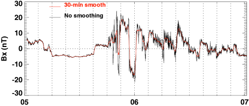
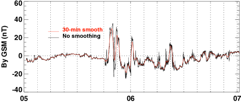
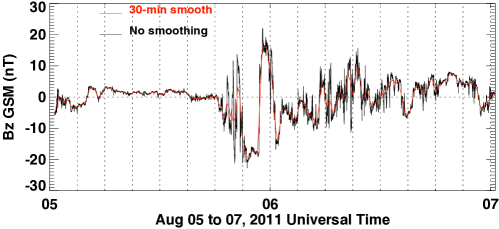
Figure 3: Observed values (black) of the hemispheric power in $10^{9}$ W (one giga Watt) and of the IMF components $B_{x}$, $B_{y}$, and $B_{z}$ and their 30-min smoothed variations (red) from 5 to 7 August 2011.

Figure 2 shows that the components of ${\bf B}_{IMF}$ and the solar wind are highly variable during the August storm. The solar wind influences the magnetosphere which in turn affects the thermosphere-ionosphere. These processes modify the upper atmosphere in addition to the effects of the direct solar input. To assess the response of the thermosphere in the presence of highly variable forcing can be a challenging task. Models provide the capability of conducting controlled simulations to diagnose the effects of different dynamical processes on the system.

We first conduct a “benchmark” simulation based on the average values during August 1–5 of the observed geomagnetic parameters with hemispheric power (HP) of $3.68$ GW, $B_{x}=1.42$ nT, $B_{y}=-1.57$ nT, $B_{z}=-0.85$ nT and solar wind speed of $v_{x}\approx 363$ km s^-1. GITM is run with these constant values from 1 to 5 August 0000 UT and the last output (5 August 0000 UT) is saved as a starting point (start-up time) for the subsequent simulations. Then, two model simulations have been conducted from 5 to 7 August 0000 UT, covering the storm period. First, with the configuration of the steady (benchmark) run and second, 30-minute smoothed observed IMF data are used as inputs as shown in Figure 3 with red lines, while the black line represents the actual observations. This smoothing enables us to focus on the larger-scale variations of the magnetosphere and subsequently determine the overall response of the thermosphere to the geomagnetic storm rather than to the small-scale temporal variations that are seen in observations. While there is large temporal variability in the actual observations, smoothing gives a general picture of how geomagnetic parameters vary. Small-scale temporal variability during storms is the subject of our future modeling efforts.

5 High-Latitude Ionospheric Convection

During geomagnetic storms, the collisionless solar wind with velocity ${\bf v}_{sw}$ distorts the Earth’s magnetic field significantly. The solar wind induced magnetospheric electric field ${\bf E}$ in Earth’s frame of reference is

$${\bf E}=-{\bf v}_{sw}\times{\bf B},$$ (1)

which is mapped down to the polar cap ionosphere. An increase in the solar wind speed and/or magnetic field ${\bf B}$ leads to an increase in ${\bf E}$. Electric fields originating from the magnetosphere make the plasma “convect” at high-latitudes and can accelerate the ions to relatively large speeds of more than 1 km s^-1 (Crowley et al., 1989). An accurate representation of ionospheric flow patterns largely driven by the magnetosphere is crucial for the investigation of the response of the thermosphere-ionosphere system to geomagnetic storms. The convection patterns depend highly on the IMF direction and magnitude (Bekerat et al., 2003). While a southward directed IMF impacts plasma convection greatly in polar latitudes, a non-zero IMF $B_{y}$ generated asymmetric thermospheric response to geomagnetic activity (Yamazaki et al., 2015).

5.1 High-Latitude Mean Ion Flows

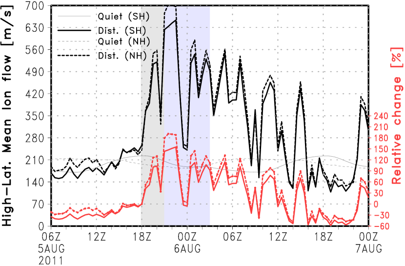
Figure 4: High-latitude means of horizontal ion flow at 400 km from 0600 UT 5 August to 0000 UT 7 August. Benchmark and storm simulations are represented by thin and thick lines. Solid and dashed lines denote Southern and Northern Hemisphere high-latitude means, respectively. Red lines show the relative percentage changes with respect to the storm onset time (1800 UT, 5 August.). Each tick mark on the time axis represent 2-hour intervals. The initial and the main phases of the storm are shaded with gray and blue, respectively.

Because the primary influence of the storm is expected to occur in the ionosphere, which coexists with the thermosphere, we first investigate the ion flow patterns in the high-latitude ionosphere. Figure 4 shows how the high-latitude means of the horizontal ion flows $|{\bf v_{i_{\rm H}}}|$ change at 400 km as a function of time from 5 August 0600 UT, that is, starting about 12 hours before the onset of the storm, to 7 August 0000 UT. The gray and blue shadings mark the initial and the main phases of the storm, respectively. The high-latitude means that are to be presented in the rest of the paper are calculated taking into account data poleward of (geographic) 60^∘N/S. Thin and thick lines represent “quiet” (benchmark) and “storm” (disturbed) runs, respectively, while solid and dashed lines show the Southern and Northern Hemispheres results, respectively. The red lines show the relative percentage change with respect to the storm onset (1800 UT, 5 August).

Under quiet conditions, the mean ion flows in the Northern and Southern Hemispheres vary diurnally with similar magnitudes but are slightly time-shifted with respect to each other primarily because of the offset between the geographic and geomagnetic poles. In the disturbed run, before the storm onset $|{\bf v_{i_{\rm H}}}|$ has similar magnitude as the benchmark run. As the storm commences, the shift in the UT variation of the mean ion flows in the different hemispheres is subdued as the IMF variations are the dominant driver of the ion flows. The response of the ionosphere is immediate in both hemispheres. Within the first 2 hours of the storm, the mean $|{\bf v}_{\rm{i}_{H}}|$ increases from 240 m s^-1 to $\sim$ 500 m s^-1 and to 560 m s^-1 in the Southern and Northern Hemispheres, respectively, corresponding to $\sim$ 100 % and $>120$% relative increase. In the main phase of the storm at around 2200 UT 5 August where the southward IMF is at its maximum (Figure 3), the mean $|{\bf v_{i_{\rm H}}}|$ reaches a maximum for the entire simulation period: to $\sim$630 m s^-1 and $>700$ m s^-1 in the Southern and Northern Hemispheres, respectively, corresponding to $\sim 150\%$ and $\sim 200\%$ relative increases. The mean $|{\bf v_{i_{\rm H}}}|$ then gradually decreases in a similar rate in both hemispheres but remains generally large during the main phase and the recovery phase of the storm.

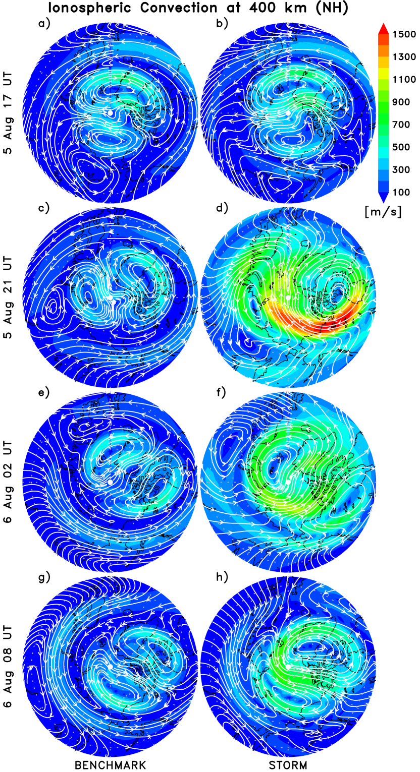
Figure 5: Northern Hemisphere ionospheric convection patterns at 400 km at four representative UTs on 5-6 August poleward of 51.25^∘ (geographic). Color shading is the magnitude of the horizontal ion flows in m s^-1. Left column is for the benchmark run, while the right column is for the storm run. The Greenwich Meridian is at the top of the plot.

5.2 High-Latitude Convection Patterns

We next investigate how the details of the ion convection patterns evolve during the storm by depicting four representative UTs. Although the high-latitude means of $|{\bf v_{i_{\rm H}}}|$ in the different hemispheres demonstrate relatively small differences in magnitude with respect to each other, the actual patterns of ion convection can differ greatly primarily because the offsets between the geographic and geomagnetic poles are different in the two hemispheres.

Figures 5 and 6 present the ionospheric convection patterns at 400 km in the Northern Hemisphere and Southern Hemispheres poleward of $\pm 51.25^{\circ}$ (geographic), respectively. White streamlines represent the horizontal ion flow structures and color shading is the magnitude of the horizontal ion speed $|{\bf v_{i_{\rm H}}}|$. The benchmark run and the storm run are shown in the left and right columns, respectively. Four representative UTs are chosen to illustrate how the convection patterns evolve: (1) 1700 UT 5 August, immediately before the storm onset, (2) 2100 UT 5 August, main phase, (3) 0200 UT 6 August, main phase, and (4) 0800 UT 6 August, recovery phase.

Before the storm onset in the Northern Hemisphere, the horizontal ion flows are in the storm simulation are similar to the benchmark run. This similarity applies both to the geographical structure and peak magnitudes of up to 500 m s^-1. There is a dominant two-cell pattern at high-latitudes with a smaller single cell pattern at lower latitudes. Under quiet constant geomagnetic conditions, the pattern merely co-rotates as a function of time while peak flow speeds do not change much. In the storm simulation, however, remarkable variations are seen in the structure and magnitude of ${\bf v_{i_{\rm H}}}$. Ion flow speeds exceed 1600 m s^-1 during the main phase of the storm (panel d) within the sustained two-cell convection pattern that has now greatly expanded, suppressing the third cell. During the recovery phase of the storm maximum ion flows of up to 1100 m s^-1 are retained in the high-latitudes.

Similar ionospheric response is seen in the Southern Hemisphere high-latitudes (Figure 6). The dominance of the two-cell pattern is present under both quiet and storm-time conditions, but a significant expansion of the two-cell pattern is seen during the main and the recovery phases of the storm. Ion flow magnitudes exceed 1600 m s^-1 within the center of the two-cell pattern whose center is now much more offset with respect to the geographic South Pole.

Remarkable response of the ion flow speeds and structure is seen in both hemispheres to the geomagnetic storm. However, overall, it is noteworthy that there exists hemispheric asymmetry during quiet periods as well as during all phases of the storm. We next focus on the thermospheric response to the storm.

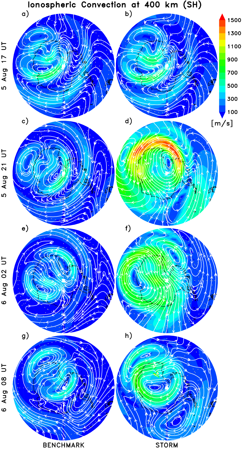
Figure 6: Same as Figure 5, but for the Southern Hemisphere poleward of $-51.25^{\circ}$. The Greenwich Meridian is at the bottom of the plot.

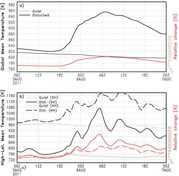
Figure 7: Variations of a) global mean and b) high-latitude mean (poleward of $\pm 60^{\circ}$) neutral temperature $T$ [K] from 5 August 0600 UT to 7 August 0000 UT at 400 km. Benchmark and storm simulations are represented by thin and thick lines. In panel b, solid and dashed lines denote Southern and Northern Hemisphere high-latitude means, respectively. Red lines show the relative percentage changes with respect to the storm onset time (1800 UT, 5 August.)

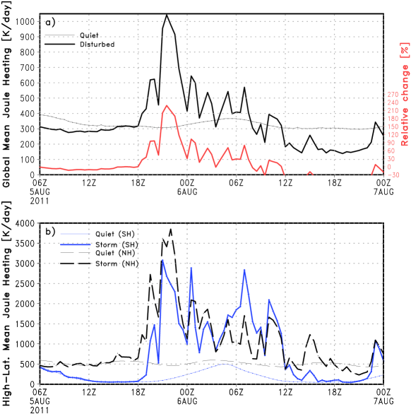
Figure 8: Variations of a) global mean and b) high-latitude mean Joule heating in K day^-1 shown in the same manner as Figure 7.

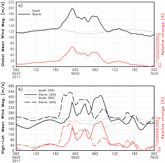
Figure 9: Same as Figure 7, but for the neutral wind magnitude.

6 Upper Atmosphere Response

6.1 Global Mean Neutral Temperature and Winds

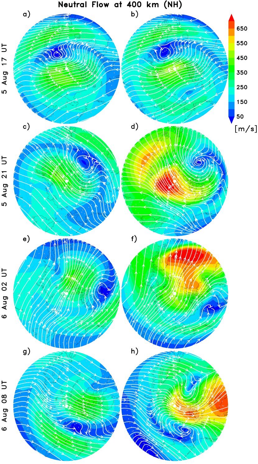
Figure 10: Same as Figure 5, but for the Northern Hemisphere neutral horizontal wind flow.

The high-latitude ionosphere under the influence of enhanced ion convection can be a significant source of energy and momentum for the thermosphere. Figures 7a,b show how the global mean and high-latitude means of the neutral temperature $T$ change at 400 km as a function of time from 5 August 0600 to 7 August 0000 UT. As the storm commences at around 1800 UT (5 August), the global mean temperature increases rapidly until 0600 UT on 6 August by 140 K ($\sim 15\%$) from 820 K to $\sim$960 K shown by the thick black line. In comparison, the global mean $T$ varies by about $\sim$10 K ($\sim 1\%$) in the same period (thin black line) in the quiet (benchmark) run.

In August, the Southern and Northern Hemispheres are the winter and summer hemispheres, respectively, and have different dynamical and thermal characteristics. To quantify how the storm affects the different hemispheres, we evaluate the high-latitude means of neutral temperature poleward of $\pm 60^{\circ}$. Under quiet geomagnetic conditions, the summer NH (thin dashed line) is about 200 K warmer than the winter SH (thin solid line) and the mean temperature varies smoothly (diurnally) during the simulated period. Similarly, the storm simulation shows about 225 K temperature difference between the different hemispheres before the storm onset.

When the storm begins, the temperatures rapidly increase in both hemispheres (thick lines), but the winter Southern Hemisphere peak thermal response to the storm (with respect to the onset time) is two times stronger than the summer Northern Hemisphere response: up to 40% vs. $\sim$20% situated at around 0500 UT on 6 August, 11 hours after the storm onset. In terms of the absolute magnitude of the thermal response, the peak temperature increase is $\sim$300 K in the winter Southern Hemisphere while it is $\sim$170 K in the summer Northern Hemisphere.

Heating of the upper atmosphere by Joule dissipation is one of the major contributors to the energy budget of the high-latitude thermosphere (Wilson et al., 2006). Joule heating $Q_{J}$ is proportional to ionization and the square of the ion-neutral differential motion (Johnson and Heelis, 2005; Yiğit and Ridley, 2011a). Figure 8 shows the associated neutral gas heating via Joule heating at 400 km in the same manner as the temperature plot in Figure 7. During quiet times, the global mean Joule heating varies smoothly between 300-400 K day^-1 over the presented period. After the onset of the storm the global mean Joule heating increases by more than a factor of three ($>200\%$) from $\sim 300$ to more than 1000 K day^-1, peaking in the main phase of the storm. At the high-latitudes approximately a factor of six increase is seen in the summer Northern Hemisphere, and more than an order of magnitude increase in the winter Southern Hemisphere. Overall, the largest increases are seen during the initial and the main phase of the storm coincident with the rapid enhancements of the ionospheric convection that can contribute to the Joule heating (Johnson and Heelis, 2005). These values suggest that instantaneously the mean Joule heating values at high-latitudes can exceed the mean solar heat input, which is typically around 1500 K day^-1.

Similar analysis is used for the case of neutral horizontal wind magnitude $|{\bf u_{H}}|=u_{H}$ and we present the corresponding results in Figure 9. This investigation should provide an overview of how the mean thermospheric circulation overall responds to the storm. In the benchmark run (thin black line), the global mean $|{\bf u_{H}}|$ varies smoothly around 120 m s^-1. Before the storm, storm-time winds are similar to the benchmark run winds. However, within six hours of the storm, global mean horizontal wind magnitude increases $>50$ % from $\sim$130 m s^-1 to $\sim$200 m s^-1. There is a secondary local peak at around 5-6 UT on 6 August, after which the system returns gradually to quiet conditions. Overall, the response of the high-latitudes seen in Figure 9b is more rapid, intensive, and variable. Although, the wind magnitude increases rapidly in both hemispheres, there is a distinct difference in the timing of the peak response to the storm in the different hemispheres. In the NH, within the first three hours of the storm, $|{\bf u_{H}}|$ increases by 80%, which is the maximum NH response during the entire storm time. On the other hand, SH high-latitude mean $|{\bf u_{H}}|$ demonstrates the largest increase at around 8 UT on 6 August that slightly exceeds the magnitude of the peak NH response during the onset phase.

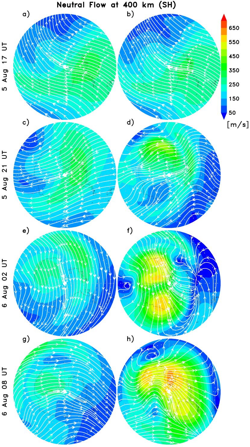
Figure 11: Same as Figure 6, but for the Southern Hemisphere neutral wind flow.

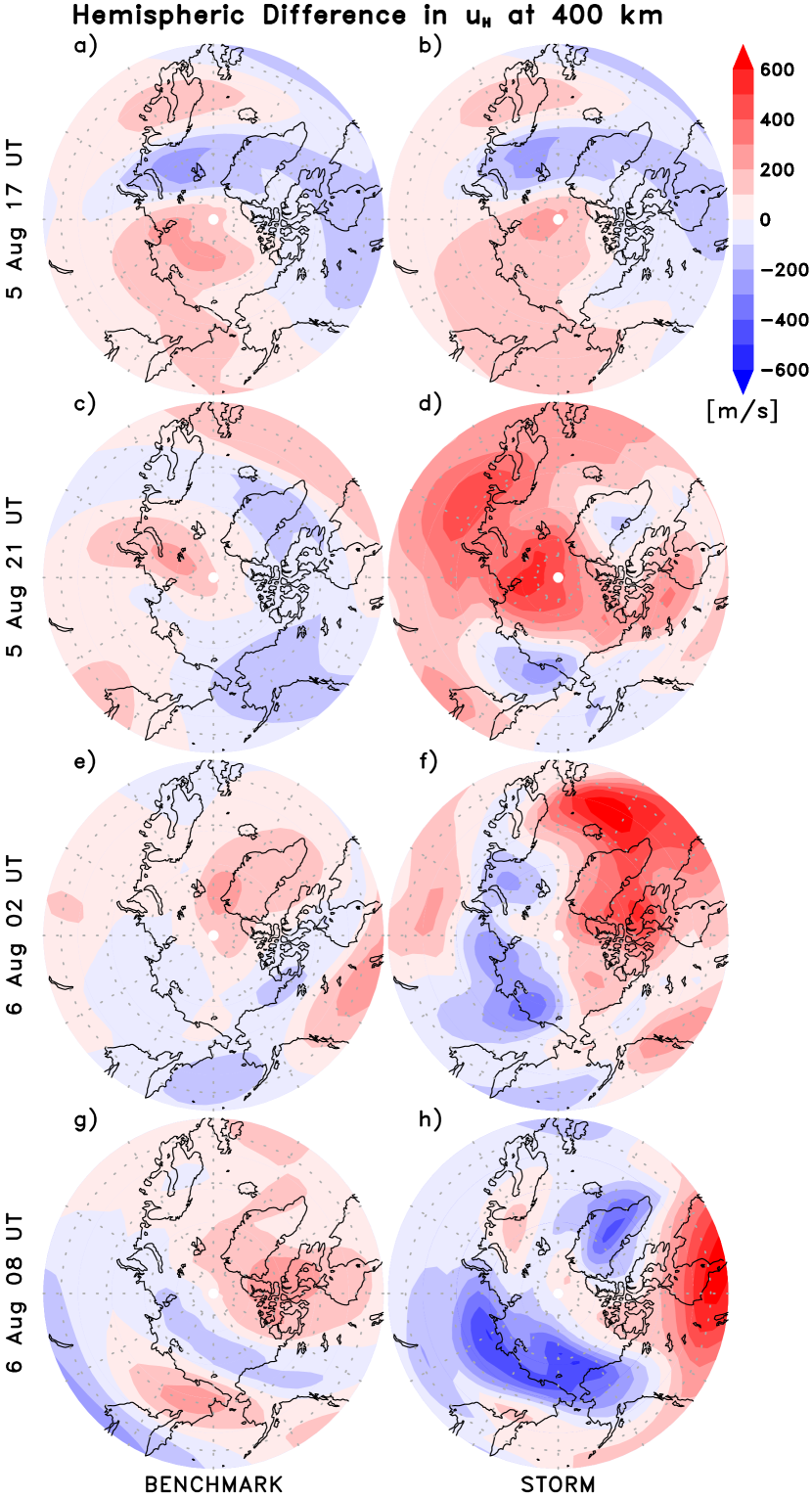
Figure 12: Hemispheric difference in the neutral horizontal wind calculated as the difference between the conjugate latitudes (Southern Hemisphere value minus Northern Hemisphere) shown poleward of $51.25^{\circ}$. The Northern Hemisphere background map is kept for reference.

6.2 Effects on the Thermospheric Circulation

To investigate the effect of the geomagnetic storm on the upper atmosphere, we next study the evolution of the thermospheric circulation at high-latitudes during the different phases of the storm. Figures 10 and 11 present the magnitude of horizontal neutral wind $u_{H}$ (shaded) combined with the neutral flow streamlines (white) in the Northern and Southern Hemisphere high-latitudes, respectively, at 400 km, similar to the way ion convection patterns were presented in Figures 5 and 6.

In the Northern summer Hemisphere, the thermospheric circulation before the onset of the storm closely resembles the benchmark (quiet) simulation (Figures 10a–b) with peak $u_{H}$ of up to 450 m s^-1. The circulation pattern is characterized primarily by the injective streamlines ($u_{h}(t_{0})\neq u_{h}(t_{1})$) of a day-to-night flow that is maintained by the pressure difference and is modified at high-latitudes by the ion drag. There is also a small region of periodic motion in a region of small $u_{H}$ close to the geographic North Pole. As the storm commences, though, we can see a dramatic increase in the neutral flow speeds with magnitudes exceeding 700 m s^-1, while the benchmark simulation demonstrates a neutral circulation whose structure co-rotates with the local time variations and the peak flow speeds remains unchanged (left column, i.e., panels a, c, e, and g). In the recovery phase of the storm, regions of large neutral flows are still present.

The Southern Hemisphere results shown in Figure 11 are overall analogous to the Northern Hemisphere results. However, we need to note two important aspects. First, horizontal flows are slightly weaker in the winter hemisphere as the pressure forces are smaller. Also, the Southern Hemisphere response to the storm occurs later than the Northern Hemisphere. Before the storm onset, the Southern Hemisphere circulation is very similar to the benchmark case. Even, in the beginning of the main phase, the results are similar to the benchmark case. Only at the end of the main phase, the thermospheric circulation is enhanced in the winter hemisphere and can still be large during the recovery phase (panel h). This behavior is consistent with the high-latitude mean neutral wind speeds (Figure 9).

7 Storm-Induced Hemispheric Difference in the Thermosphere

Storm-time evolution of the thermospheric circulation suggests that the summer and winter hemispheres respond differently to the storm in terms of plasma and neutral flow magnitudes and timing. We next investigate how the differences in the thermospheric circulation between the two hemispheres evolve with the occurrence of the storm.

In order to evaluate the hemispheric differences in the circulation of the thermosphere, which we broadly term as hemispheric asymmetry, we first calculate the quantity $\Delta u_{H}$: For every longitude grid point, we define the hemispheric difference as the difference $\Delta f$ between the value of a parameter $f$ at two conjugate latitude points with respect to the geographic equator (i.e., Southern Hemisphere values minus Northern Hemisphere value). If all conjugate latitude grid points are included, then a latitude-longitude distribution of $\Delta f$ can be obtained.

The results are shown in Figure 12. The panels are structured in the same way as in Figures 10 and 11. We have kept the Northern Hemisphere background map for the purpose of convenience. Evolution of $\Delta u_{H}$ in the quiet-time run (left panels) suggest first that there is some degree of geographical difference between the hemispheres ($\pm 200$ m s^-1) in the absence of a storm, due primarily to the seasonal differences. Second, the amount of the difference does not change much during the period under consideration in the benchmark run; the structure rotates as a function of UT. On the other hand, during the storm $\Delta u_{H}$ values are overall much larger and exceed values of $\pm 600$ m s^-1. The peak magnitude of these differences is larger than the peak high-latitude mean horizontal wind (c.f., Figure 9b). The storm-induced rapid enhancement of the hemispheric difference is clearly illustrated by comparing $\Delta u_{H}$ before and after the storm onset (panels b and d). The peak difference values increase by a factor of 4 to 5. During the different phases of the storm, the magnitude as well as the structure of the hemispheric difference evolves in a complex manner. The difference in the dynamical response timing of the different hemispheres is a major factor that contributes to the hemispheric asymmetry at a given time.

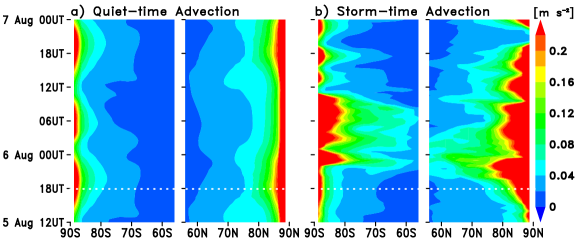
Figure 13: Temporal evolution of horizontal advective forcing at 400 km in the a) benchmark (left two panels) and b) the storm (right two panels) simulations. Units are in m s^-2. White dotted line marks the storm onset.

8 Discussion

The geomagnetic field ${\bf B}_{E}$ is consistently directed northward (i.e., from the South Pole to the North Pole). When a strong southward interplanetary magnetic field (IMF) $B_{IMF}$ ($B_{z}<0$) arrives at the magnetosphere, the IMF undergoes reconnection, allowing the two field lines to connect temporarily. These processes can enhance energy transfer from the solar wind to the magnetosphere down to the thermosphere-ionosphere system, producing geomagnetic storms. Accordingly, our simulations show that the large ionospheric convection encountered in the main phase of the August 2011 storm coincides with periods of large negative IMF ($B_{z}<0$).

The asymmetric offset between the geographic and geomagnetic axes produces substantial differences in the momentum and heating sources in the upper atmosphere, greatly contributing to hemispheric differences in the structure and composition of the ionosphere and thermosphere. In August, the Northern Hemisphere is the summer hemisphere, while the Southern Hemisphere is in winter. Therefore, a certain degree of difference will be present because of the seasonal (solar irradiation) differences between the hemispheres when the geomagnetic storm occurs.

In our simulations, remarkable dynamical changes are seen in the thermospheric circulation, following the rapid changes in the ionospheric convection due to the enhanced electric fields of magnetospheric origin, which influence the ion drift motion ${\bf v_{i}}$ given approximately by

$${\bf v}_{{\bf E}\times{\bf B}}=\frac{{\bf E}\times{\bf B}}{|{\bf B}|^{2}}.$$ (2)

Overall, the structure of the simulated ion convection patterns are consistent with the previously observed (e.g., Bristow et al., 2011) and modeled (Killeen and Roble, 1984; Heppner and Maynard, 1987) patterns at high-latitudes. During $B_{z}<0$ conditions, the large-scale structure of this convection is characterized by anti-sunward flow over the polar cap and return flow at auroral latitudes.

Changes in the general circulation of the thermosphere occur during the storm due primarily to the variations in the pressure and ion drag forcings. These are two major dynamical mechanisms that shape the neutral flow. During a geomagnetic storm the neutral temperature is enhanced which modulates the pressure force. On the other hand, enhanced ion flows (Figures 4–6) can drive the neutrals to higher speeds via increased ion drag effect. Storm-time increased conductivities and electric fields lead to an increase in the current density. From the point of thermospheric dynamics, ion motion is viewed in terms of drift velocities. Therefore the momentum exchange between the ions and neutrals is proportional to their differential velocity ${\bf v_{i}}-{\bf u}$. At high-latitudes, ions possess larger speeds and can thus impart an ion drag force on the neutrals. Increased neutral flows can then produce additional nonlinear dynamical response in the system in the later stages of the storm because of advective processes.

Based on the above dynamical analysis, the structure and the evolution of the simulated hemispheric differences in the thermospheric circulation can be interpreted qualitatively as the following. In the earlier stages of the storm, enhanced ion flows drive the neutrals to larger speeds, to a different degree in the different hemispheres. By the beginning of the recovery phase of the storm, the thermospheric circulation has become stronger and therefore, nonlinear processes in the neutral flow, such as wind advection, sustain large winds and contribute to hemispheric differences. The associated horizontal wind advection is shown in Figure 13, where the UT-latitude cross-sections of the horizontal advective forcing of the neutral horizontal circulation are shown for the quiet-time (panel a) and the storm-time (panel b) simulations, respectively. The advective forcing is enhanced appreciable during the storm and is characterized by a marked hemispheric asymmetry in terms of its spatiotemporal variations. In this context, our simulations support the conclusions of Förster et al. (2008) that a non-zero $B_{y}$ is likely to contribute to an asymmetry in the thermosphere. During the storm, substantial fluctuations are seen in $B_{y}$ as well. Recently, Yamazaki et al. (2015) have highlighted the importance of the $B_{y}$ effect in structure of the thermosphere.

The models of Fuller-Rowell and Rees (1980) and Dickinson et al. (1981) were the first of their kind in terms of three-dimensional modeling of the thermosphere. They have used simplified ionospheres represented by the Chiu (1975) empirical ionosphere model and the configuration of Earth’s geomagnetic field has been simplified by a dipole field. One of the first studies of thermospheric circulation during geomagnetic storms was conducted by Fuller-Rowell and Rees (1981) for idealized conditions of a substorm specified by the variation of the $K_{p}$ index from 1 to 6. Their simulation covered a period of 4.5 h. Wind speeds exceeding 600 m s^-1  were seen at around 400 km. In our study we have used the measured storm-time IMF values from the ACE satellite in order to specify the configuration of the high-latitude electric fields.

Recently, the works by Haaser et al. (2013), Earle et al. (2013), Gong et al. (2013), and Huang et al. (2014) have studied the low-latitude dynamics during the August 2011 storm using global satellite observations and incoherent scatter radar (ISR) data. Gong et al. (2013)’s analysis of Arecibo ISR data showed profound meridional wind enhancements in the low-latitude thermosphere. Also, Earle et al. (2013) showed, using the Air Force Communication/Navigation Outage Forecasting System (C/NOFS) satellite, an increase in the neutral horizontal flows during the storm. Our simulations have shown that the global mean horizontal neutral winds are overall enhanced (up to 50 %) during the storm and this increase is even more pronounced in the high-latitudes (up to 80%). Our results are consistent with these observations.

9 Summary and Conclusions

Using the three-dimensional nonhydrostatic Global Ionosphere Thermosphere Model (GITM) driven by the observed solar and geomagnetic activity input from satellites, dynamical and thermal response of the thermosphere and ionosphere to the 5–6 August 2011 major geomagnetic storm has been quantified and new physical insights to the challenging problem of hemispheric differences have been provided. We have analyzed the major ion and neutral parameters during the storm. Specifically, high-latitude mean ion and neutral flows, global mean temperature, polar stereographic projections of the ion and neutral flows in the Northern and Southern Hemispheres have been evaluated during the different phases of the storm and are compared to quiet-time simulations. The magnitude of hemispheric differences in the thermospheric circulation has been determined and interpreted by calculating nonlinear advective forcing. Polar stereographic projections have been performed for representative storm periods: Immediately before the storm onset, main storm phase, and the recovery phase. The main findings are:

(1) Storm-induced changes in the ionosphere show rapid and large enhancement of ion flows with the onset of the storm and the simulated ion convection patterns are consistent with previous modeling and observational studies;

(2) Thermospheric circulation changes are appreciable during the storm. The response of the neutrals to the storm is a slower process, owing to their larger inertia. The global mean neutral temperature increases by up to $15\%$. At high-latitudes, the thermal response of the Southern winter Hemisphere is overall two times larger than the Northern summer Hemisphere: $30\%$ vs. $15\%$. The global mean neutral wind magnitude increases up to $50\%$ and up to $80\%$ in the high-latitude mean winds. The response of the neutral winds in the winter Southern Hemisphere occurs later than in the summer Northern Hemisphere; and

(3) Substantial hemispheric differences are seen during the storm in the thermospheric circulation resulting from ion-neutral coupling effects and nonlinear dynamical changes. Comparison with quiet-time simulations suggest that storm-time hemispheric differences are at least a factor of two larger and highly variable during the different phases of the storm.

(4) Especially in the recovery phase of the storm, a significant degree of hemispheric difference is seen in the global circulation of the thermosphere. Modeled nonlinear advective processes in the neutral horizontal flows demonstrate substantial differences between the two hemispheres, suggesting that advective forcing plays an important role in maintaining hemispheric differences in the thermosphere.

Here, we have not included the effects of lower atmospheric small-scale waves on the upper atmosphere as the model lower boundary is around the mesopause. Gravity waves propagate to the upper atmosphere (Yiğit et al., 2008; Gavrilov and Kshevetskii, 2013) and produce appreciable dynamical (Yiğit et al., 2009, 2012b) and thermal effects (Yiğit and Medvedev, 2009) on the general circulation of the thermosphere up to F-region altitudes. Thermospheric gravity wave effects exhibit substantial solar cycle variations (Yiğit and Medvedev, 2010). Under moderate major geomagnetic storm conditions, the dynamical effects of internal waves on the upper atmosphere are probably of minor significance at the altitudes ($\sim 400$ km) studied in this paper. However, a detailed quantification of internal wave effects on the upper atmosphere during geomagnetic storms is yet to be done. Global models extending into the upper atmosphere (e.g., Yiğit et al., 2009) or in general, whole atmosphere models (e.g., Jin et al., 2011; Akmaev, 2011) could be used to study internal wave effects at higher altitudes in conjunction with space weather effects.

One limitation of our simulations is the use of the empirical model of Weimer (1996). Empirical models provide a gross (mean) structure of the atmosphere and do not include the realistic variability of the upper atmosphere. Empirical ionospheric convection models, specifically, provide an average structure of high-latitude convection patterns, based on a large collection of observations (Bekerat et al., 2003). The principle is similar to the distribution of neutral winds modeled by empirical wind models (e.g., Hedin et al., 1996) or the solar irradiance models (Tobiska et al., 2000). Empirical models are broadly used in the aeronomy community due to their simplicity and portability.

In future investigations, assimilative modeling techniques could provide a better ground for representing (small-scale) variability at high-latitudes during disturbed geomagnetic conditions. A comparison of convection patterns obtained from the Assimilative Mapping of Ionospheric Electrodynamics technique (AMIE, Richmond and Kamide, 1988) with patterns retrieved from the DMSP satellite showed that AMIE patterns matched the observations better than statistical models (Bekerat et al., 2005). Future research on storm-induced thermospheric variations could utilize the AMIE technique.

References

- Abdu et al. (2006) Abdu, M. A., T. K. Ramkumar, I. S. Batista, C. G. M. Brum, H. Takahashi, B. W. Reinisch, and J. H. A. Sobral (2006), Planetary wave signatures in the equatorial atmosphere-ionosphere system, and mesosphere-e- and f-region coupling, J. Atmos. Sol.-Terr. Phys., 68, 509–522.
- Akmaev (2011) Akmaev, R. A. (2011), Whole atmosphere modeling: Connecting terrestrial and space weather, Rev. Geophys., 49, RG4004.
- Altadill et al. (2004) Altadill, D., E. M. Apostolov, J. Boška, J. Laštovička, and P. Šauli (2004), Planetary and gravity wave signatures in the F-region ionosphere with impact on radio propagation predictions and variability, Ann. Geophys., 47, 1109–1119.
- Anderson et al. (1998) Anderson, B. J., J. B. Gary, T. A. Potemra, R. A. Frahm, J. R. Sharber, and J. D. Wahington (1998), Uars observationos of Birkeland currents and Joule heating rates for the November 4, 1993, storm, J. Geophys. Res., 103, 26,323–26,335.
- Anderson et al. (2011) Anderson, C., T. Davies, M. Conde, P. Dyson, and M. J. Kosch (2011), Spatial sampling of the thermospheric vertical wind field at auroral latitudes, J. Geophys. Res., 116, A07305.
- Balan et al. (2011) Balan, N., M. Yamamoto, J. Y. L. nad Y. Otsuka, H. Liu, and H. Lühr (2011), New aspects of thermospheric and ionospheric storms revealed by CHAMP, J. Geophys. Res., 116, A06320, doi:10.1029/2010JA016399.
- Balan et al. (2012) Balan, N., J. Y. Liu, Y. Otsuka, S. T. Ram, and H. Lühr (2012), Ionospheric and thermospheric storms at equatorial latitudes observed by CHAMP, ROCSAT, and DMSP, J. Atmos. Sci., 117, A01313, doi:10.1029/2011JA016903.
- Bekerat et al. (2003) Bekerat, H. A., R. W. Schunk, and L. Scherliess (2003), Evaluation of statistical convection patterns for real-time ionospheric specifications and forecasts, J. Geophys. Res., 108(A12), doi:10.1029/2003JA009945.
- Bekerat et al. (2005) Bekerat, H. A., R. W. Schunk, L. Scheirles, and A. Ridley (2005), Comparison of satellite ion drift velocities with AMIE derived convection patterns, J. Atmos. Sol.-Terr. Phys., 67, 1463–1479.
- Blanch et al. (2013) Blanch, E., S. Marsal, A. Segarra, J. M. Torta, D. Altadill, and J. J. Curto (2013), Space weather effects on earth’s environment associated to the 24–25 October 2011 geomagnetic storm, Space Weather, 11, 153–168, doi:10.1002/swe.20035.
- Bristow (2008) Bristow, W. (2008), Statistics of velocity fluctuations observed by SuperDARN under steady interplanetary magnetic field conditions, J. Geophys. Res., 113, A11202, doi:10.1029/2008JA013203.
- Bristow et al. (2011) Bristow, W. A., J. Spaleta, and R. T. Parris (2011), First observations of ionospheric irregularities and flows over the south geomagnetic pole from the super dual auroral radar network (SuperDARN) hf radar at mcmurdo station, antarctica, J. Geophys. Res., 116, A12325, doi:10.1029/2011JA016834.
- Burns et al. (2012) Burns, A. G., S. C. Solomon, L. Qian, W. Wang, B. A. Emery, M. Wiltberger, and D. R. Weimer (2012), The effects of Corotating interaction region/High speed stream storms on the thermosphere and ionosphere during the last solar minimum, J. Atmos. Sol.-Terr. Phys., 83, 79–87, doi:10.1016/J.JASTP.2012.02.006.
- Chiu (1975) Chiu, Y. T. (1975), An improved phenomenological model of ionospheric density, J. Atmos. Terr. Phys., 37, 1563–1570.
- Crowley et al. (1989) Crowley, G., B. A. Emery, R. G. Roble, H. C. Carlson, and D. J. Knipp (1989), Thermospheric dynamics during september 18-19, 1984 1. model simulations, J. Geophys. Res., 94(A12), 16,925–16,944.
- Deng et al. (2008) Deng, Y., A. D. Richmond, A. J. Ridley, and H. Liu (2008), Assessment of the non-hydrostatic effect on the upper atmosphere using a general circulation model (GCM), Geophys. Res. Lett., 35, L01104, doi:10.1029/2007GL032182.
- Dickinson et al. (1981) Dickinson, R. E., E. C. Ridley, and R. G. Roble (1981), A three-dimensional general circulation model of the thermosphere, J. Geophys. Res., 86(A3), 1499–1512.
- Dungey (1961) Dungey, J. W. (1961), Interplanetary magnetic field and the auroral zones, Phys. Rev. Lett., 6(2), 47–48.
- Earle et al. (2013) Earle, G. D., R. L. Davidson, R. A. Heelis, W. R. Coley, D. R. Weimer, J. J. Makela, D. J. Fisher, A. J. Gerrard, and J. Meriwether (2013), Low latitude thermospheric responses to magnetic storms, J. Geophys. Res., 118, doi:10.1002/jgra.50212.
- Emery et al. (1999) Emery, B. A., C. Lathuillere, P. G. Richards, R. G. Roble, M. J. Buonsanto, D. J. Knippe, P. Wilkinson, D. P. Sipler, and R. Niciejewski (1999), Time dependent thermospheric neutral response to the 2-11 November 1993 storm period, J. Atmos. Sol.-Terr. Phys., 61, 329–350.
- Förster et al. (2008) Förster, M., S. Rentz, W. Köhler, H. Liu, and S. E. Haaland (2008), IMF dependence of high-latitude thermospheric wind pattern derived from CHAMP cross-track measurements, Ann. Geophys., 26, doi:10.5194/angeo-26-1581-2008.
- Fuller-Rowell and Evans (1987) Fuller-Rowell, T. J., and D. S. Evans (1987), Height-integrated Pederson and Hall conductivity patterns inferred from TIROS-NOAA satellite data, J. Geophys. Res., 92, 7606–7618.
- Fuller-Rowell and Rees (1980) Fuller-Rowell, T. J., and D. Rees (1980), A three dimensional time-dependent global model of the thermosphere, J. Atmos. Sci., 37, 2545–2567.
- Fuller-Rowell and Rees (1981) Fuller-Rowell, T. J., and D. Rees (1981), A three-dimensional, time-dependent simulation of the global dynamical response of the thermosphere to a geomagnetic storm, J. Atmos. Terr. Phys., 43(7), 701–721.
- Gavrilov and Kshevetskii (2013) Gavrilov, N. M., and S. P. Kshevetskii (2013), Numerical modeling of propagation of breaking nonlinear acoustic-gravity waves from the lower to the upper atmosphere, Adv. Space Res., 51, 1168–1174, doi:10.1016/j.asr.2012.10.023.
- Gong et al. (2013) Gong, Y., Q. Zhou, S. D. Zhang, N. Aponte, M. Sulzer, and S. Gonzalez (2013), The F region and topside ionosphere response to a strong geomagnetic storm at Arecibo, J. Geophys. Res., 118, 5177–5183, doi:10.1002/jgra.50502.
- Gonzalez et al. (1994) Gonzalez, W. D., J. A. Joselyn, Y. Kamide, H. W. Kroehl, G. Rostoker, B. T. Tsurutani, and V. M. Vasyliunas (1994), What is a geomagnetic storm?, J. Geophys. Res., 99(A4), 5771–5792.
- Haaser et al. (2013) Haaser, R. A., R. Davidson, R. A. Heelis, G. D. Earle, S. Venkatraman, and J. Klenzing (2013), Storm time meridional wind perturbations in the equatorial upper thermosphere, J. Geophys. Res. Space Physics, 118, doi:10.1002/jgra.50299.
- Hagan and Forbes (2002) Hagan, M. E., and J. M. Forbes (2002), Migrating and nonmigrating diurnal tides in the middle and upper atmosphere excited by tropospheric latent heat release, J. Geophys. Res., 107(D24), 4754, doi:10.1029/2001JD001236.
- Hagan and Forbes (2003) Hagan, M. E., and J. M. Forbes (2003), Migrating and nonmigrating semidiurnal tides in the middle and upper atmosphere excited by tropospheric latent heat release, J. Geophys. Res., 108(A2), 1062, doi:10.1029/2002JA009466.
- Hedin et al. (1996) Hedin, A. E., E. L. Fleming, A. H. Manson, F. J. Schmidlin, S. K. Avery, R. R. Clark, S. J. Franke, G. J. Fraser, T. Tsuda, F. Vial, and R. A. Vincent (1996), Empirical wind model for the upper, middle and lower atmosphere, J. Atmos. Terr. Phys., 58, 1421–1447.
- Heppner and Maynard (1987) Heppner, J. P., and N. C. Maynard (1987), Empirical high-latitude electric field models, J. Geophys. Res., 92(A5), 4467–4489, doi:10.1029/JA092iA05p04467.
- Huang et al. (2014) Huang, C. Y., Y.-J. Su, E. K. Sutton, D. R. Weimer, and R. L. Davidson (2014), Energy coupling during the august 2011 magnetic storm, J. Geophys. Res. Space Physics, 119, doi:10.1002/2013JA019297.
- Immel et al. (2001) Immel, T. J., G. Crowley, J. D. Craven, and R. G. Roble (2001), Dayside enhancements of thermospheric O/N2 following magnetic storm onset, J. Geophys. Res., 106, 15,471–15,488.
- Innis and Conde (2002) Innis, J. L., and M. Conde (2002), High-latitude thermospheric vertical wind activity from Dynamics Explorer 2 Wind and Temperature Spectrometer observations: Indications of a source region for polar cap gravity waves, J. Geophys. Res., 107, A81172, doi:10.1029/2001JA009130.
- Jin et al. (2011) Jin, H., Y. Miyoshi, H. Fujiwara, H. Shinagawa, K. Terada, N. Terada, M. Ishii, Y. Otsuka, and A. Saito (2011), Vertical connection from the tropospheric activities to the ionospheric longitudinal structure simulated by a new earth’s whole atmosphere-ionosphere coupled model, J. Geophys. Res. Space Physics, 116(A1), doi:10.1029/2010JA015925.
- Johnson and Heelis (2005) Johnson, E. S., and R. A. Heelis (2005), Characteristics of ion velocity structure at high latitudes during steady southward interplanetary magnetic field conditions, J. Geophys. Res., 110, A12301, doi:10.1029/2005JA011130.
- Kil et al. (2011) Kil, H., Y.-S. Kwak, L. J. Paxton, R. R. Meier, and Y. Zhang (2011), O and N2 disturbances in the F region during the 20 November 2003 storm seen from TIMED/GUVI, J. Geophys. Res., 116, A02314, doi:10.1029/2010JA016227.
- Killeen and Roble (1984) Killeen, T. L., and R. G. Roble (1984), An analysis of the high-latitude thermospheric wind pattern calculated by a thermospheric general circulation model 1. momentum forcing, J. Geophys. Res., 89, 7509–7522.
- Klimenko and Klimenko (2012) Klimenko, M., and V. Klimenko (2012), Disturbance dynamo, prompt penetration electric field and overshielding in the earth’s ionosphere during geomagnetic storm, J. Atmos. Sol.-Terr. Phys., 90–91(0), 146 – 155, doi:http://dx.doi.org/10.1016/j.jastp.2012.02.018, recent Progress in the Vertical Coupling in the Atmosphere-Ionosphere System.
- Lu et al. (2013) Lu, G., J. D. Huba, and C. Valladares (2013), Modeling ionospheric super-fountain effect based on the coupled TIMEGCM-SAMI3, J. Geophys. Res. Space Physics, 118, 2527–2535, doi:10.1002/jgra.50256.
- Ma et al. (2012) Ma, Y., C. Shen, V. Angelopoulos, A. Lui, X. Li, H. U. Frey, M. Dunlop, and D. L. H.U. Auster, J.P. McFadden (2012), Tailward leap multiple expansions of the plasma sheet during a moderately intense substorm: Themis observations, J. Geophys. Res., 117, A07219, doi:2012JA017768.
- Mannucci et al. (2005) Mannucci, A. J., B. T. Tsurutani, B. A. Iijima, A. Komjathy, A. Saito, W. D. Gonzalez, F. L. Guarnieri, J. U. Kozyra, and R. Skoug (2005), Dayside global ionospheric response to the major interplanetary events of October 29–30, 2003 Halloween Storms, Geophys. Res. Lett., 32(12), doi:10.1029/2004GL021467, l12S02.
- Martyn (1951) Martyn, D. F. (1951), The theory of magnetic storms and auroras, Nature, 167, 92–94.
- Matsuo et al. (2003) Matsuo, T., A. D. Richmond, and K. Hensel (2003), High-latitude ionospheric electric field variability and electric potential derived from DE-2 plasma drift measurements: Dependence on IMF and dipole tilt, J. Geophys. Res., 108(A1), 1005, doi:10.1029/2002JA009429.
- Oliver et al. (1988) Oliver, W. L., S. Fukao, T. Sato, T. Tsuda, S. Kato, I. Kimura, A. Ito, T. Saryou, and T. Araki (1988), Ionospheric incoherent scatter measurements with the middle and upper atmosphere radar: Observations during the large magnetic storm of february 6-8, 1986, J. Geophys. Res., 93, 14,649–14,655.
- Pancheva and Mukhtarov (2011) Pancheva, D., and P. Mukhtarov (2011), Stratospheric warmings: The atmosphere-ionosphere coupling paradigm, J. Atmos. Sol.-Terr. Phys., 73, 1697–1702.
- Pancheva et al. (2009) Pancheva, D., P. Mukhtarov, B. Andonov, N. J. Mitchell, and J. M. Forbes (2009), Planetary waves observed by TIMED/SABER in coupling the stratosphere–mesosphere–lower thermosphere during the winter of 2003/2004: Part 1—comparison with the UKMO temperature results, J. Atmos. Sol.-Terr. Phys., 71, 61–74, doi:10.1016/j.jastp.2008.09.016.
- Pawlowski and Ridley (2009) Pawlowski, D. J., and A. J. Ridley (2009), Modeling the ionospheric response to the 28 October 2003 solar flare due to coupling with the thermosphere, R. Sci., 44, RS0A23, doi:10.1029/2008RS004081.
- Prölss (2011) Prölss, G. W. (2011), Density perturbations in the upper atmosphere caused by the dissipation of solar wind energy, Surv. Geophys., 32, doi:10.1007/s10712-010-9104-0.
- Richmond and Kamide (1988) Richmond, A. D., and Y. Kamide (1988), Mapping electrodynamic features of the high-latitude ionosphere from localized observations: Technique, J. Geophys. Res., 93, 5741–5759.
- Richmond and Matsushita (1975) Richmond, A. D., and S. Matsushita (1975), Thermospheric response to a magnetic substorm, J. Geophys. Res., 80(19), 2839–2850.
- Ridley et al. (2006) Ridley, A. J., Y. Deng, and G. Tóth (2006), The global ionosphere–thermosphere model, J. Atmos. Sol.-Terr. Phys., 68, 839–864.
- Roble et al. (1982) Roble, R. G., R. E. Dickinson, and E. C. Ridley (1982), Global circulation and temperature structure of thermosphere with high-latitude plasma convection, J. Geophys. Res., 87, 1599–1614.
- Tobiska et al. (2000) Tobiska, W. K., T. Woods, F. Eparvier, R. Viereck, L. Floyd, D. Bouwer, G. Rottman, and O. R. White (2000), The solar2000 empirical solar irradiance model and forecast tool, J. Atmos. Sol.-Terr. Phys., 62, 1233–1250.
- Vichare et al. (2012) Vichare, G., A. Ridley, and E. Yiğit (2012), Quiet-time low latitude ionospheric electrodynamics in the non-hydrostatic global ionosphere–thermosphere model, J. Atmos. Sol.-Terr. Phys., 80, 161–172, doi:10.1016/j.jastp.2012.01.009.
- Weimer (1996) Weimer, D. (1996), A flexible, IMF dependent model of high-latitude electric potentials having space weather application, Geophys. Res. Lett., 23, 2549–255.
- Wilson et al. (2006) Wilson, G. R., D. R. Weimer, J. O. Wise, and F. A. Marcos (2006), Response of the thermosphere to Joule heating and particle precipitation, J. Geophys. Res., A10314, doi:10.1029/2005JA011274.
- Yamazaki et al. (2015) Yamazaki, Y., M. J. Kosch, and E. K. Sutton (2015), North-south asymmetry of the high-latitude thermospheric density: IMF BY effect, Geophys. Res. Lett., 42(2), 225–232, doi:10.1002/2014GL062748.
- Yiğit and Medvedev (2009) Yiğit, E., and A. S. Medvedev (2009), Heating and cooling of the thermosphere by internal gravity waves, Geophys. Res. Lett., 36, L14807, doi:10.1029/2009GL038507.
- Yiğit and Medvedev (2010) Yiğit, E., and A. S. Medvedev (2010), Internal gravity waves in the thermosphere during low and high solar activity: Simulation study., J. Geophys. Res., 115, A00G02, doi:10.1029/2009JA015106.
- Yiğit and Medvedev (2015) Yiğit, E., and A. S. Medvedev (2015), Internal wave coupling processes in Earth’s atmosphere, Adv. Space Res., 55, 983–1003, doi:10.1016/j.asr.2014.11.020.
- Yiğit and Ridley (2011a) Yiğit, E., and A. J. Ridley (2011a), Effects of high-latitude thermosphere heating at various scale sizes simulated by a nonhydrostatic global thermosphere-ionosphere model, J. Atmos. Sol.-Terr. Phys., 73, 592–600, doi:10.1016/j.jastp.2010.12.003.
- Yiğit and Ridley (2011b) Yiğit, E., and A. J. Ridley (2011b), Role of variability in determining the vertical wind speeds and structure, J. Geophys. Res., 116, A12305, doi:10.1029/2011JA016714.
- Yiğit et al. (2008) Yiğit, E., A. D. Aylward, and A. S. Medvedev (2008), Parameterization of the effects of vertically propagating gravity waves for thermosphere general circulation models: Sensitivity study, J. Geophys. Res., 113, D19106, doi:10.1029/2008JD010135.
- Yiğit et al. (2009) Yiğit, E., A. S. Medvedev, A. D. Aylward, P. Hartogh, and M. J. Harris (2009), Modeling the effects of gravity wave momentum deposition on the general circulation above the turbopause, J. Geophys. Res., 114, D07101, doi:10.1029/2008JD011132.
- Yiğit et al. (2012a) Yiğit, E., A. J. Ridley, and M. B. Moldwin (2012a), Importance of capturing heliospheric variability for studies of thermospheric vertical winds, J. Geophys. Res., 117, A07306, doi:10.1029/2012JA017596.
- Yiğit et al. (2012b) Yiğit, E., A. S. Medvedev, A. D. Aylward, A. J. Ridley, M. J. Harris, M. B. Moldwin, and P. Hartogh (2012b), Dynamical effects of internal gravity waves in the equinoctial thermosphere, J. Atmos. Sol.-Terr. Phys., 90–91, 104–116, doi:10.1016/j.jastp.2011.11.014.
- Zaka et al. (2010) Zaka, K. Z., A. T. Kobea, V. Doumbia, A. D. Richmond, A. Maute, N. M. Mene, O. K. Obrou, P. Assamoi, K. Boka, J.-P. Adohi, and C. Amory-Mazaudier (2010), Simulation of electric field and current during the 11 june 1993 disturbance dynamo event: Comparison with the observations, J. Geophys. Res. Space Physics, 115(A11), doi:10.1029/2010JA015417.