Information transmission over an amplitude damping channel with an arbitrary degree of memory

Abstract

We study the performance of a partially correlated amplitude damping channel acting on two qubits. We derive lower bounds for the single-shot classical capacity by studying two kinds of quantum ensembles, one which allows to maximize the Holevo quantity for the memoryless channel and the other allowing the same task but for the full-memory channel. In these two cases, we also show the amount of entanglement which is involved in achieving the maximum of the Holevo quantity. For the single-shot quantum capacity we discuss both a lower and an upper bound, achieving a good estimate for high values of the channel transmissivity. We finally compute the entanglement-assisted classical channel capacity.

I Introduction

One of the key issues of quantum information is the use of quantum systems to convey information. Although quantum systems are unavoidably affected by noise, reliable transmission is still possible by proper coding cover-thomas ; nielsen-chuang ; benenti-casati-strini ; wilde . Coding involves multiple channel uses. The relevant quantities for classical and quantum information transmission are the classical capacity hausladen ; schumacher-westmoreland ; holevo98 $C$ and the quantum capacity lloyd ; barnum ; devetak $Q$, defined as the maximum number of, respectively, bits and and qubits that can be reliably transmitted per channel use. Finally, the entanglement-assisted classical capacity adami-Cerf ; bennett1999 ; bennett-shor $C_{E}$ is the capacity of transmitting classical information, provided the sender and the receiver share unlimited prior entanglement. This latter quantity is important since it upper bounds the previous ones. We have $Q\leq C\leq C_{E}$. The computation of capacities $C$ and $Q$ is in general a hard task, since a “regularization” procedure is requested, namely an optimization over all possible $n$-use input states, in the limit $n\to\infty$.

In the simplest setting each channel use is independent of the previous ones. It means that, if a quantum channel use is described by the map $\mathcal{E}$, $n$ uses of the channel are described by the map $\mathcal{E}_{n}=\mathcal{E}^{\otimes n}$. This assumption is not always justified. For instance, with increasing the transmission rate, the environment may retain memory of the previous channel uses. In this case noise introduces memory (or correlation) effects among consecutive channel uses, and $\mathcal{E}_{n}\neq\mathcal{E}^{\otimes n}$ (memory channels). Such effects can be investigated experimentally in optical fibers banaszek or in solid-state implementations of quantum hardware, affected by low-frequency noise solid-state . Quantum memory channels attracted growing interest in the last years, and interesting new features emerged thanks to modeling of relevant physical examples, including depolarizing channels mp02 ; MMM , Pauli channels mpv04 ; daems ; dc , dephasing channels hamada ; njp ; virmani ; gabriela ; lidar , Gaussian channels cerf , lossy bosonic channels mancini ; lupo , spin chains spins , collision models collision , complex network dynamics caruso , and a micromaser model micromaser . For a recent review on quantum channels with memory effects, see Ref. memo_review .

Here we study the behavior of a two-qubit memory amplitude damping channel. We extend the model introduced in Ref. MADC2013 by addressing the cases of partial memory. We use a memory parameter $\mu$ which spans from zero to one allowing us to recover the memoryless case ($\mu=0$) as well as the full memory case ($\mu=1$). We study the channel capability to transmit both classical and quantum information as well as the entanglement-assisted classical information. We derive lower bounds for the classical capacity, lower and upper bounds for the quantum capacity, and compute the channel capacity for entanglement-assisted classical communication. In all cases we analytically indentify a general form of the ensembles that optimize the channel capacities. Then we perform numerical optimizations for single use of the channel, thus deriving lower bounds for $Q$ and $C$, as well as computing $C_{E}$, for which the regularization $n\to\infty$ is not needed. For such ensembles, we also show the populations of the density operators which solve the optimization problems. Such information may provide useful indications for real (few channel uses) coding strategies. In the case of the classical capacity, we investigate two classes of ensembles; we find that neither of them is useful to overcome -for the memoryless setting- the limit of the product state classical capacity of the (memoryless) amplitude damping channel giovannetti ; hastings . Finally, we find that any finite amount of memory increases the amount of reliably transmitted information with respect to the memoryless case, for all the scenarios considered.

The paper is organized as follows. In Sec. II we describe the channel model and the channel covariance properties. In Sec. III we study the classical capacity of the quantum channel, addressing the ensembles classes which maximize the Holevo quantity, showing two distinct lower bounds for the classical capacity. In Sec. IV we compute both a lower and an upper bound for the quantum capacity, which are very close to each other for good quality (relatively high transmissivity) channels. In V we determine the quantum capacity and the entanglement-assisted channel capacity. We finish with concluding remarks in Sec. VI.

II The Model and its covariance properties

We will first briefly review the memoryless amplitude damping channel (ad) nielsen-chuang ; benenti-casati-strini , which acts on a generic single-qubit state $\rho$ as follows:

$$\rho\quad\rightarrow\quad\rho^{\prime}={\cal E}(\rho)\,=\,\sum_{i\in\{0,1\}}E_{i}\,\rho\,E_{i}^{\dagger},$$ (1)

where the Kraus operators $E_{i}$ are given by

$${E}_{0}=\left(\begin{array}[]{cc}1&0\\ 0&\sqrt{\eta}\\ \end{array}\right),\qquad{E}_{1}=\left(\begin{array}[]{cccc}0&\sqrt{1-\eta}\\ 0&0\\ \end{array}\right).$$ (2)

Here we are using the orthonormal basis $\{|{0}\rangle,|{1}\rangle\}$ ($\sigma_{z}=|{0}\rangle\langle{0}|-|{1}\rangle\langle{1}|$). This channel describes relaxation processes, such as spontaneous emission of an atom, in which the system decays from the excited state $|{1}\rangle$ to the ground state $|{0}\rangle$. The channel acts as follows on a generic single-qubit state:

$$\rho=\left(\begin{array}[]{cc}1-p&\gamma\\ \gamma*&p\\ \end{array}\right)\quad\rightarrow\quad\rho^{\prime}={\cal E}(\rho)=\left(\begin{array}[]{cc}1-\eta\,p&\sqrt{\eta}\,\gamma\\ \sqrt{\eta}\,\gamma*&\eta\,p\\ \end{array}\right).$$ (3)

Note that the noise parameter $\eta$ ($0\leq\eta\leq 1$) plays the role of channel transmissivity. Indeed for $\eta=1$ we have a noiseless channel, whereas for $\eta=0$ the channel cannot carry any information since for any possible input we always obtain the same output state $|{0}\rangle$.

For two memoryless uses we have that

$$\rho\quad\rightarrow\quad\rho^{\prime}={\cal E}_{0}(\rho)\,=\,\sum_{i\in\{0,3\}}A_{i}\,\rho\,A_{i}^{\dagger},$$ (4)

where $\rho$ is the density matrix related to a two-qubit system, and ${\cal E}_{0}={\cal E}\otimes{\cal E}$ so that the Kraus operators $A_{i}$ are given by

$$A_{0}=E_{0}\otimes E_{0}=\left(\begin{array}[]{cccc}1&0&0&0\\ 0&\sqrt{\eta}&0&0\\ 0&0&\sqrt{\eta}&0\\ 0&0&0&\eta\\ \end{array}\right),$$ (9)

$$A_{1}=E_{0}\otimes E_{1}=\left(\begin{array}[]{cccc}0&\sqrt{1-\eta}&0&0\\ 0&0&0&0\\ 0&0&0&\sqrt{\eta(1-\eta)}\\ 0&0&0&0\\ \end{array}\right),$$ (14)

$$A_{2}=E_{1}\otimes E_{0}=\left(\begin{array}[]{cccc}0&0&\sqrt{1-\eta}&0\\ 0&0&0&\sqrt{\eta(1-\eta)}\\ 0&0&0&0\\ 0&0&0&0\\ \end{array}\right),$$ (19)

$$A_{3}=E_{1}\otimes E_{1}=\left(\begin{array}[]{cccc}0&0&0&1-\eta\\ 0&0&0&0\\ 0&0&0&0\\ 0&0&0&0\\ \end{array}\right).$$ (24)

For two channel uses, a full-memory amplitude damping channel was introduced in Ref. yeo and recently investigated in Ref. Jahangir ; MADC2013

$$\rho\quad\rightarrow\quad\rho^{\prime}={\cal E}_{1}(\rho)\,=\,\sum_{i}B_{i}\,\rho\,B_{i}^{\dagger},$$ (25)

with the Kraus operators

$${B}_{0}=\left(\begin{array}[]{cccc}1&0&0&0\\ 0&1&0&0\\ 0&0&1&0\\ 0&0&0&\sqrt{\eta}\\ \end{array}\right),\,\,{B}_{1}=\left(\begin{array}[]{cccc}0&0&0&\sqrt{1-\eta}\\ 0&0&0&0\\ 0&0&0&0\\ 0&0&0&0\\ \end{array}\right).$$ (26)

In ${\cal E}_{1}$ the relaxation phenomena are fully correlated. In other words, when a qubit undergoes a relaxation process, the other qubit does the same. In this way only the state $|{11}\rangle\equiv|{1}\rangle\otimes|{1}\rangle$ can decay, while the other states $|{ij}\rangle\equiv|{i}\rangle\otimes|{j}\rangle$, $i,j\,\in\,\{0,1\}$, $ij\neq 11$, are not affected.

In this paper we will focus on the partially correlated channel ${\cal E}_{\mu}$, defined as a convex combination of the memoryless channel ${\cal E}_{0}$ and the full memory channel ${\cal E}_{1}$

$$\rho\quad\rightarrow\quad\rho^{\prime}={\cal E}_{\mu}(\rho)\,=\,(1-\mu){\cal E}_{0}(\rho)+\mu\,{\cal E}_{1}(\rho).$$ (27)

Here, $\mu\,\in\,[0,1]$ is the memory parameter: the memoryless channel (${\cal E}_{0}$) is recovered when $\mu=0$, whereas for $\mu=1$ we obtain the “full memory” amplitude damping channel (${\cal E}_{1}$). In the following, we will derive lower bounds for the single-shot classical capacity $C_{1}({\cal E}_{\mu})$, lower and upper bounds for the quantum capacity $Q({\cal E}_{\mu})$, and we will compute the entanglement-assisted classical capacity $C_{E}({\cal E}_{\mu})$.

We will now investigate some covariance properties of the above channel, that will be subsequently exploited to derive the above mentioned bounds. We define the following unitary operators:

$${\cal R}_{1}=\sigma_{z}\otimes\openone,\quad{\cal R}_{2}=\openone\otimes\sigma_{z},\quad{\cal R}_{3}=\sigma_{z}\otimes\sigma_{z}.$$ (28)

It is straightforward to demonstrate that the operators $A_{i}$ (24) and $B_{i}$ (26) either commute or anticommute with ${\cal R}_{i}$ (28), namely

$$A_{0}{\cal R}_{i}={\cal R}_{i}A_{0},\quad B_{0}{\cal R}_{i}={\cal R}_{i}B_{0},\quad\forall\,i\,\in\{1,2,3\},$$ (29)

$${\cal R}_{1}A_{1}\,=\,A_{1}{\cal R}_{1},\quad{\cal R}_{2}A_{1}\,=\,-A_{1}{\cal R}_{2},\quad{\cal R}_{3}A_{1}\,=\,-A_{1}{\cal R}_{3},$$ (30)

$${\cal R}_{1}A_{2}\,=\ -A_{2}{\cal R}_{1},\quad{\cal R}_{2}A_{2}\,=\,A_{2}{\cal R}_{2},\quad{\cal R}_{3}A_{2}\,=\,-A_{2}{\cal R}_{3},$$ (31)

$${\cal R}_{3}A_{2}\,=\,-A_{3}{\cal R}_{1},\quad{\cal R}_{2}A_{3}\,=\,-A_{3}{\cal R}_{2},\quad{\cal R}_{3}A_{2}\,=\,A_{3}{\cal R}_{3},$$ (32)

$${\cal R}_{1}B_{1}\,=\,-B_{1}{\cal R}_{1},\quad{\cal R}_{2}B_{1}\,=\,-B_{1}{\cal R}_{2},\,\quad{\cal R}_{3}B_{1}\,=\,B_{1}{\cal R}_{3}.$$ (33)

¿From the above relations it follows that

$${\cal E}_{0}({\cal R}_{1}\,\rho\,{\cal R}_{1})\,=\,\sum_{i=0}^{3}A_{i}{\cal R}_{1}\,\rho\,{\cal R}_{1}A_{i}^{\dagger}\,=$$

$$=\,{\cal R}_{1}A_{0}\rho A_{0}{\cal R}_{1}\,+\,{\cal R}_{1}A_{1}\rho{\cal R}_{1}A^{\dagger}_{1}\,+\,$$

$$\hskip 28.45274pt+(-{\cal R}_{1}A_{2})\rho(-A^{\dagger}_{2}{\cal R}_{1})\,+\,(-{\cal R}_{1}A_{3})\rho(-A^{\dagger}_{3}{\cal R}_{1})\,=$$

$$=\,{\cal R}_{1}\Big{(}\sum_{i}A_{i}\,\rho\,A_{i}^{\dagger}\Big{)}{\cal R}_{1}\,={\cal R}_{1}\,{\cal E}_{0}(\rho)\,{\cal R}_{1},$$ (34)

where we use

$$A^{\dagger}_{0}=A_{0},$$

$${\cal R}_{1}A^{\dagger}_{1}=(A_{1}{\cal R}_{1})^{\dagger},=({\cal R}_{1}A_{1})^{\dagger}=A_{1}^{\dagger}{\cal R}_{1},$$

$${\cal R}_{1}A^{\dagger}_{2}=(A_{2}{\cal R}_{1})^{\dagger}=(-{\cal R}_{1}A_{2})^{\dagger}=-A_{2}^{\dagger}{\cal R}_{1},$$

$${\cal R}_{1}A^{\dagger}_{3}=(A_{3}{\cal R}_{1})^{\dagger}=(-{\cal R}_{1}A_{3})^{\dagger}=-A_{3}^{\dagger}{\cal R}_{1}.$$

In a similar way it can be shown that ${\cal E}_{0}({\cal R}_{2}\,\rho\,{\cal R}_{2})={\cal R}_{2}\,{\cal E}_{0}(\rho)\,{\cal R}_{2}$ and ${\cal E}_{0}({\cal R}_{3}\,\rho\,{\cal R}_{3})={\cal R}_{3}\,{\cal E}_{0}(\rho)\,{\cal R}_{3}$: the channel ${\cal E}_{0}$ is covariant with respect to all the operators ${\cal R}_{i}$. With a similar argument it can be proved that also the full memory channel ${\cal E}_{1}$ is covariant with respect to ${\cal R}_{i}$ MADC2013 . Therefore, also the channel with an arbitrary degree of memory is covariant with respect to ${\cal R}_{i}$, namely

$${\cal E}_{\mu}({\cal R}_{i}\rho{\cal R}_{i})=(1-\mu)\,{\cal R}_{i}{\cal E}_{0}(\rho){\cal R}_{i}\,+\,\mu\,{\cal R}_{i}{\cal E}_{1}(\rho){\cal R}_{i}={\cal R}_{i}{\cal E}_{\mu}(\rho){\cal R}_{i}.$$ (35)

Now we consider the action of the Swap gate nielsen-chuang , defined as

$${\cal S}_{\textrm{w}}\equiv|{00}\rangle\langle{00}|\,+\,|{01}\rangle\langle{10}|\,+\,|{10}\rangle\langle{01}|\,+\,|{11}\rangle\langle{11}|.$$ (36)

We notice that

$${\cal S}_{\textrm{w}}\,A_{0}\,{\cal S}_{\textrm{w}}\,=\,A_{0},\quad{\cal S}_{\textrm{w}}\,A_{1}\,{\cal S}_{\textrm{w}}\,=\,A_{2},\quad{\cal S}_{\textrm{w}}\,A_{2}\,{\cal S}_{\textrm{w}}\,=\,A_{1},\quad{\cal S}_{\textrm{w}}\,A_{3}\,{\cal S}_{\textrm{w}}\,=\,A_{3}.$$ (37)

By using ${\cal S}_{\textrm{w}}^{\dagger}={\cal S}_{\textrm{w}}$, ${\cal S}_{\textrm{w}}{\cal S}_{\textrm{w}}=\openone$ and the above relations, we can easily prove that the channel ${\cal E}_{0}$ is covariant with respect to ${\cal S}_{\textrm{w}}$, namely

$${\cal E}_{0}({\cal S}_{\textrm{w}}\,\rho\,{\cal S}_{\textrm{w}})\,=\,{\cal S}_{\textrm{w}}\,{\cal E}_{0}(\rho)\,{\cal S}_{\textrm{w}}\;.$$ (38)

It is straightforward to demonstrate that ${\cal S}_{\textrm{w}}$ commutes with the Kraus operators $B_{0}$ and $B_{1}$ (26). Therefore the channel ${\cal E}_{1}$ is covariant with respect to ${\cal S}_{\textrm{w}}$. Since both the channels ${\cal E}_{0}$ and ${\cal E}_{1}$ are covariant with respect to ${\cal S}_{\textrm{w}}$, the channel ${\cal E}_{\mu}$ is also covariant under the action of ${\cal S}_{\textrm{w}}$.

III Classical capacity

In this section we will study the performance of the channel to transmit classical information, quantified by the classical capacity $C$, that measures the maximum amount of classical information that can be reliably transmitted down the channel per channel use. More specifically, we address the problem of computing the single shot capacity $C_{1}$ nielsen-chuang of the partially correlated channel ${\cal E}_{\mu}$, that is achieved by maximizing the so called Holevo quantity $\chi$ nielsen-chuang ; benenti-casati-strini ; holevo73 ; schumacher-westmoreland ; holevo98 ; hausladen with respect to one use of the channel ${\cal E}_{\mu}$ as follows:

$$C_{1}({\cal E}_{\mu})=\max_{\{p_{\alpha},\rho_{\alpha}\}}{\chi\big{(}{\cal E}\mu,\{p_{\alpha},\rho_{\alpha}\}\big{)}}.$$ (39)

In the above expression $\{p_{\alpha},\rho_{\alpha}\}$ is a quantum source, described by the density operator $\rho=\sum_{\alpha}p_{\alpha}\rho_{\alpha}$ and the Holevo quantity is defined as

$$\chi\big{(}{\cal E}\mu,\{p_{\alpha},\rho_{\alpha}\}\big{)}\equiv S({\cal E}\mu(\rho))\,-\,\sum_{\alpha}p_{\alpha}S({\cal E}\mu(\rho_{\alpha})),$$ (40)

where $S(\rho)=-{\rm Tr}(\rho\log_{2}\rho)$ is the von Neumann entropy. Without loss of generality, in the following we will restrict to ensembles of pure states $\{p_{k},|{\psi_{k}}\rangle\}$, since any ensemble of mixed states can be described by an ensemble of pure states with same density operator, and whose Holevo quantity (40) is at least as large schumacher-westmoreland . The above expressions then become

$$C_{1}({\cal E}\mu)=\max_{\{p_{k},|{\psi_{k}}\rangle\}}{\chi\big{(}{\cal E}\mu,\{p_{k},|{\psi_{k}}\rangle\}\big{)}},$$ (41)

$$\chi\big{(}{\cal E}\mu,\{p_{k},|{\psi_{k}}\rangle\}\big{)}\,=$$

$$\hskip 14.22636pt=\,S({\cal E}\mu(\rho))\,-\,\sum_{k}p_{k}S({\cal E}\mu(|{\psi_{k}}\rangle\langle{\psi_{k}}|)),$$ (42)

where now $\rho=\sum_{k}\,p_{k}|{\psi_{k}}\rangle\langle{\psi_{k}}|$. The optimization of $C_{1}$ was performed for the amplitude damping channel with full memory ($\mu=1$) in Ref. MADC2013 . The case of partial memory is harder to treat, so in the following we will derive lower bounds on $C_{1}$, by exploiting the channel covariance properties discussed above and employing specific ensembles.

III.1 Form of optimal ensembles

We derive here a general form of the ensemble that optimizes the Holevo quantity, by exploiting the covariance properties discussed in the previous section. First we take advantage of the covariance property of the channel ${\cal E}_{\mu}$ with respect to ${\cal R}_{i}$ (28). Given a generic ensemble $\{p_{k},|{\psi_{k}}\rangle\}$, we consider a new ensemble by replacing each state $|{\psi_{k}}\rangle$ in $\{p_{k},|{\psi_{k}}\rangle\}$ by the set

$$\{|{\psi_{k}}\rangle,\,{\cal R}_{1}|{\psi_{k}}\rangle,\,{\cal R}_{2}|{\psi_{k}}\rangle,\,{\cal R}_{3}|{\psi_{k}}\rangle\},$$

each state occurring with probability $\tilde{p}_{k}=p_{k}/4$. We refer to this new ensemble as $\{\tilde{p}_{k},|{\tilde{\psi}_{k}}\rangle\}$, and call $\tilde{\rho}=\sum_{k}\tilde{p}_{k}|{\tilde{\psi}_{k}}\rangle\langle{\tilde{\psi}_{k}}|$ the associated density operator

$$\tilde{\rho}\,=\,\sum_{k}\frac{p_{k}}{4}\Big{(}|{\psi_{k}}\rangle\langle{\psi_{k}}|\,+\,\sum_{i=1}^{3}{\cal R}_{i}|{\psi_{k}}\rangle\langle{\psi_{k}}|{\cal R}_{i}\Big{)}\,=$$

$$=\frac{1}{4}\Big{(}\rho\,+\,\sum_{i=1}^{3}{\cal R}_{i}\rho{\cal R}_{i}\Big{)}.$$ (43)

It can be verified that $\tilde{\rho}$ has the same diagonal elements of $\rho$, while the off-diagonal entries are all vanishing. We now show that

$$\chi\big{(}{\cal E}\mu,\{\tilde{p}_{k},|{\tilde{\psi}_{k}}\rangle\}\big{)}\geq\chi\big{(}{\cal E}\mu,\{p_{k},|{\psi_{k}}\rangle\}\big{)}.$$ (44)

To this end we first notice that

$$S\big{(}{\cal E}\mu({\cal R}_{i}|{\psi_{k}}\rangle\langle{\psi_{k}}|{\cal R}_{i})\big{)}\,=\,S\big{(}{\cal R}_{i}\,{\cal E}\mu(|{\psi_{k}}\rangle\langle{\psi_{k}}|)\,{\cal R}_{i}\big{)}$$

$$\hskip 76.82234pt=\,S\big{(}{\cal E}\mu(|{\psi_{k}}\rangle\langle{\psi_{k}}|)\big{)},$$ (45)

where we used Eqs. (35) and the fact that a unitary operation does not change the von Neumann entropy. Therefore, by replacing the old ensemble with the new one, the second term in the Holevo quantity (42) does not change, namely

$$\sum_{k}\tilde{p}_{k}S({\cal E}\mu(|{\tilde{\psi}_{k}}\rangle\langle{\tilde{\psi}_{k}}|))\,=\,4\sum_{k}\frac{p_{k}}{4}S({\cal E}\mu(|{\psi_{k}}\rangle\langle{\psi_{k}}|))\,=\,\sum_{k}p_{k}S({\cal E}\mu(|{\psi_{k}}\rangle\langle{\psi_{k}}|)).$$ (46)

For the output entropy related to $\tilde{\rho}$ we have

$$S({\cal E}\mu(\tilde{\rho}))\,=\,S\Big{(}{\cal E}\mu\Big{(}\frac{1}{4}\rho\,+\,\frac{1}{4}\sum_{i=1}^{3}{\cal R}_{i}\rho{\cal R}_{i}\Big{)}\Big{)}\,=\,S\Big{(}\frac{1}{4}{\cal E}\mu\big{(}\rho\big{)}\,+\,\frac{1}{4}\sum_{i=1}^{3}{\cal E}\mu\big{(}{\cal R}_{i}\rho{\cal R}_{i}\big{)}\Big{)}\,$$

$$\hskip 5.69046pt\geq\frac{1}{4}S\big{(}{\cal E}\mu\big{(}\rho\big{)}\big{)}\,+\,\frac{1}{4}\sum_{i=1}^{3}S\big{(}{\cal E}\mu\big{(}{\cal R}_{i}\rho{\cal R}_{i}\big{)}\big{)}\,=\,S\big{(}{\cal E}\mu\big{(}\rho\big{)}\big{)},$$ (47)

where we used the linearity of ${\cal E}_{\mu}$, the concavity of the von Neumann entropy nielsen-chuang , and Eq. (45). Relations (46) and (47) then prove the inequality (44). In other words, for an arbitrary ensemble of pure states we can always find another ensemble, whose density matrix has the same diagonal elements as the initial ensemble and vanishing off-diagonal entries, and whose Holevo quantity is at least as large.

We will now take advantage of the covariance of the channel ${\cal E}_{\mu}$ with respect to the swap gate ${\cal S}_{\textrm{w}}$ (36). Given a quantum ensemble $\{\tilde{p}_{k},|{\tilde{\psi}_{k}}\rangle\}$, with $\tilde{\rho}=\sum_{k}\tilde{p}_{k}|{\tilde{\psi}_{k}}\rangle\langle{\tilde{\psi}_{k}}|=$   $\textrm{diag}\{\alpha,\beta,\gamma,\delta\}$, we construct a new ensemble $\{\bar{p}_{k},|{\bar{\psi}_{k}}\rangle\}$ by replacing each state $|{\tilde{\psi}_{k}}\rangle$ in $\{\tilde{p}_{k},|{\tilde{\psi}_{k}}\rangle\}$ with the following couple of states

$$\{|{\tilde{\psi}_{k}}\rangle,\,{\cal S}_{\textrm{w}}|{\tilde{\psi}_{k}}\rangle\},$$

each state occurring with probability $\bar{p}_{k}=\tilde{p}_{k}/2$. We refer to this new ensemble as $\{\bar{p}_{k},|{\bar{\psi}_{k}}\rangle\}$, and call $\bar{\rho}=\sum_{k}\bar{p}_{k}|{\bar{\psi}_{k}}\rangle\langle{\bar{\psi}_{k}}|$ the density operator which describes it. We now show that

$$\chi\big{(}{\cal E}\mu,\{\bar{p}_{k},|{\bar{\psi}_{k}}\rangle\}\big{)}\geq\chi\big{(}{\cal E}\mu,\{\tilde{p}_{k},|{\tilde{\psi}_{k}}\rangle\}\big{)}.$$ (48)

In order to do this, we first exploit the covariance property of the channel with respect to ${\cal S}_{\textrm{w}}$ (38), which leads to

$$S\big{(}{\cal E}_{\mu}({\cal S}_{\textrm{w}}|{\tilde{\psi}_{k}}\rangle\langle{\tilde{\psi}_{k}}|{\cal S}_{\textrm{w}})\big{)}\,=\,S\big{(}{\cal S}_{\textrm{w}}\,{\cal E}_{\mu}(|{\tilde{\psi}_{k}}\rangle\langle{\tilde{\psi}_{k}}|)\,{\cal S}_{\textrm{w}}\big{)}\,$$

$$\hskip 59.75095pt=\,S\big{(}{\cal E}_{\mu}(|{\tilde{\psi}_{k}}\rangle\langle{\tilde{\psi}_{k}}|)\big{)}.$$ (49)

Therefore, by replacing the old ensemble by the new one, the second term in the Holevo quantity (42) does not change, namely

$$\sum_{k}\bar{p}_{k}S({\cal E}_{\mu}(|{\bar{\psi}_{k}}\rangle\langle{\bar{\psi}_{k}}|))=2\sum_{k}\frac{\tilde{p}_{k}}{2}S({\cal E}_{\mu}(|{\tilde{\psi}_{k}}\rangle\langle{\tilde{\psi}_{k}}|))\,=\,\sum_{k}\tilde{p}_{k}S({\cal E}_{\mu}(|{\tilde{\psi}_{k}}\rangle\langle{\tilde{\psi}_{k}}|)).$$ (50)

Let us now consider the changes in the first term of the Holevo quantity (42). First we consider the relation between $\bar{\rho}$ and $\tilde{\rho}$, namely

$$\tilde{\rho}=\sum_{k}\tilde{p}_{k}|{\tilde{\psi}_{k}}\rangle\langle{\tilde{\psi}_{k}}|\rightarrow$$

$$\bar{\rho}\,=\,\sum_{k}\frac{\tilde{p}_{k}}{2}\Big{(}|{\tilde{\psi}_{k}}\rangle\langle{\tilde{\psi}_{k}}|\,+\,{\cal S}_{\textrm{w}}|{\tilde{\psi}_{k}}\rangle\langle{\tilde{\psi}_{k}}|{\cal S}_{\textrm{w}}\Big{)}=\frac{1}{2}\Big{(}\tilde{\rho}\,+\,{\cal S}_{\textrm{w}}\tilde{\rho}{\cal S}_{\textrm{w}}\Big{)}\,=$$

$$=\left(\begin{array}[]{cccc}\alpha&0&0&0\\ 0&\frac{\beta+\gamma}{2}&0&0\\ 0&0&\frac{\beta+\gamma}{2}&0\\ 0&0&0&\delta\\ \end{array}\right).$$ (55)

We have that

$$S({\cal E}_{\mu}(\bar{\rho}))\,=\,S\Big{(}{\cal E}_{\mu}\Big{(}\frac{1}{2}\tilde{\rho}\,+\,\frac{1}{2}{\cal S}_{\textrm{w}}\tilde{\rho}{\cal S}_{\textrm{w}}\Big{)}\Big{)}\,=\,S\Big{(}\frac{1}{2}{\cal E}_{\mu}\big{(}\tilde{\rho}\big{)}\,+\,\frac{1}{2}{\cal E}_{\mu}\big{(}{\cal S}_{\textrm{w}}\tilde{\rho}{\cal S}_{\textrm{w}}\big{)}\Big{)}$$

$$\hskip 22.76228pt\geq\frac{1}{2}S\big{(}{\cal E}_{\mu}\big{(}\tilde{\rho}\big{)}\big{)}\,+\,\frac{1}{2}S\big{(}{\cal E}_{\mu}\big{(}{\cal S}_{\textrm{w}}\tilde{\rho}{\cal S}_{\textrm{w}}\big{)}\big{)}\,=\,S\big{(}{\cal E}_{\mu}\big{(}\tilde{\rho}\big{)}\big{)}.$$ (56)

Relations (50) and (56) then prove inequality (48). We can summarize the above argument as follows: for any quantum ensemble of pure states we can find another ensemble, whose density matrix has the same diagonal as the original one, with zero off-diagonal entries, with equal populations for the states $|{01}\rangle$ and $|{10}\rangle$, and whose Holevo quantity is at least as large. In the following we will consider such kind of ensembles, which we will indicate by $\{p_{k},|{\psi_{k}}\rangle\}$. A generic input state $|{\psi_{k}}\rangle$ in these ensembles has the form

$$|{\psi_{k}}\rangle\,=\,a_{k}|{00}\rangle\,+\,b_{k}|{01}\rangle\,+\,c_{k}|{10}\rangle\,+\,d_{k}|{11}\rangle,$$ (57)

where the coefficients $a_{k},\,b_{k},\,c_{k},\,d_{k}\ \in\mathbb{C}$ and satisfy the normalization condition $|a_{k}|^{2}+|b_{k}|^{2}+|c_{k}|^{2}+|d_{k}|^{2}=1$. The corresponding density matrix is given by

$$\rho=\left(\begin{array}[]{cccc}\alpha&0&0&0\\ 0&\beta&0&0\\ 0&0&{\beta}&0\\ 0&0&0&\delta\\ \end{array}\right),$$ (58)

where

$$\alpha=\sum_{k}p_{k}|a_{k}|^{2},\quad{\beta}=\sum_{k}p_{k}|b_{k}|^{2}=\sum_{k}p_{k}|c_{k}|^{2},\quad\delta=\sum_{k}p_{k}|d_{k}|^{2}\,=\,1\,-\,\alpha\,-\,2{\beta}.$$ (59)

III.2 Lower bounds for $C_{1}({\cal E}_{\mu})$

Computing the $C_{1}$ capacity for the channel ${\cal E}_{\mu}$ is a very hard task since one should perform the following maximization:

$$C_{1}({\cal E}_{\mu})=\max_{\{p_{k},|{\psi_{k}}\rangle\}}\chi\big{(}{\cal E}_{\mu},\{p_{k},|{\psi_{k}}\rangle\}\big{)}$$ (60)

over all quantum ensembles $\{p_{k},|{\psi_{k}}\rangle\}$ of the form (57, 58). We will derive here some lower bounds for $C_{1}({\cal E}_{\mu})$ by optimizing the Holevo quantity of ${\cal E}_{\mu}$ with respect to some specific ensembles of the above mentioned form. We will consider two types of such ensembles.

The first ensemble, which we call ${\cal G}_{1}$, is given by the following eight states:

$$|{\psi}\rangle,\,\,{\cal R}_{i}|{\psi}\rangle,\,\,{\cal S}_{\textrm{w}}|{\psi}\rangle,\,\,{\cal R}_{i}{\cal S}_{\textrm{w}}|{\psi}\rangle,\quad i\in\{1,2,3\},$$ (61)

$$\textrm{where}\quad|{\psi}\rangle\,=\,a|{00}\rangle\,+\,b|{01}\rangle\,+\,c|{10}\rangle\,+\,d|{11}\rangle,$$ (62)

each state occurring with the same probability $p=1/8$. Here $a,b,c,d$ are complex numbers. It is straightforward to show that the resulting density matrix $\rho$ has the form (58) where

$$\alpha=|a|^{2},\quad{\beta}=\frac{|b|^{2}+|c|^{2}}{2},\quad\delta=|d|^{2}.$$ (63)

The Holevo quantity relative to the ensemble ${\cal G}_{1}$ is

$$\chi\big{(}{\cal E}_{\mu},{\cal G}_{1})\,=\,S\big{(}{\cal E}_{\mu}(\rho)\big{)}-S\big{(}{\cal E}_{\mu}(|{\psi}\rangle\langle{\psi}|)\big{)},$$ (64)

since by construction all the states in the ensemble (62) have the same output entropy, due to the covariance properties of ${\cal E}_{\mu}$ with respect to ${\cal R}_{i}$ (35) and ${\cal S}_{\textrm{w}}$ (38) exploited above. Therefore a lower bound for the classical capacity of the channel ${\cal E}_{\mu}$ can be derived from

$$\chi_{lwb_{{\cal G}_{1}}}(\eta,\mu)=\max_{a,b,c,d}\chi\big{(}{\cal E}_{\mu},{\cal G}_{1}).$$ (65)

Without loss of generality we set

$$a=\overline{a},\quad b=\overline{b}e^{i\varphi_{1}},\quad c=\overline{c}e^{i\varphi_{2}},\quad d=\sqrt{1-\overline{a}^{2}-\overline{b}^{2}-\overline{c}^{2}}\,e^{i\varphi_{3}},\,\quad\,$$

$$\textrm{and}\quad\overline{a},\,\,\overline{b},\,\,\overline{c},\,\,\varphi_{1},\,\,\varphi_{2},\,\,\varphi_{3}\in\mathbb{R}.$$ (66)

The maximization (65) can be recast as

$$\chi_{lwb_{{\cal G}_{1}}}(\eta,\mu)=\max_{\overline{a},\,\overline{b},\,\overline{c},\,\varphi_{1},\,\varphi_{2},\,\varphi_{3}}\chi\big{(}{\cal E}_{\mu},{\cal G}_{1}),$$ (67)

with the following constraints:

$$\overline{a},\,\,\overline{b},\,\,\overline{c}\,\,\in\,\,[0,1],\quad\overline{a}^{2}+\overline{b}^{2}+\overline{c}^{2}\,\leq\,1,\quad\varphi_{i}\,\,\in\,\,[0,2\pi[.$$ (68)

The reason for investigating such a lower bound is that the set ${\cal G}_{1}$ contains the ensemble which allows to achieve the product state capacity $2\,C_{madc,1}$ nielsen-chuang for two uses of the memoryless amplitude damping channel giovannetti . In the case of memoryless channel ($\mu=0$) the lower bound (65) will be at least equal to $2\,C_{madc,1}$.

The second quantum ensemble we consider is of the kind

$$\{{p}_{k},|{{\psi}_{k}}\rangle\}\,=\,\{{p}_{\varphi k},|{{\varphi}_{k}}\rangle\}\,\cup\,\{{p}_{\phi,k},|{{\phi}_{k}}\rangle\},$$ (69)

where

$$\left\{\begin{array}[]{ll}{p}_{\varphi\pm}=\beta,&|{\varphi_{+}}\rangle\,=\,\cos\theta_{1}|{01}\rangle\,+\,e^{i\varphi_{1}}\sin\theta_{1}|{10}\rangle,\\ &|{\varphi_{-}}\rangle\,=\,-\sin\theta_{1}|{01}\rangle\,+\,e^{i\varphi_{1}}\cos\theta_{1}|{10}\rangle,\\ &\\ {p}_{\phi\pm}=\frac{1-2\beta}{2},&|{\phi_{\pm}}\rangle=\cos\theta_{2}|{00}\rangle\pm e^{i\varphi_{2}}\sin\theta_{2}|{11}\rangle.\end{array}\right.$$ (74)

We call this ensemble ${\cal G}_{2}$. The corresponding density operator is

$$\rho=\left(\begin{array}[]{cccc}(1-2\beta)\cos^{2}\theta_{2}&0&0&0\\ 0&{\beta}&0&0\\ 0&0&{\beta}&0\\ 0&0&0&(1-2\beta)\sin^{2}\theta_{2}\\ \end{array}\right),$$ (75)

which is of the form (58). The Holevo quantity relative to the ensemble ${\cal G}_{2}$ is given by

$$\chi\big{(}{\cal E}_{\mu},{\cal G}_{2})\,=\,S\big{(}{\cal E}_{\mu}(\rho)\big{)}\,+$$

$$\hskip 28.45274pt-2\beta S\big{(}{\cal E}_{\mu}(|{\varphi_{\pm}}\rangle\langle{\varphi_{\pm}}|)\big{)}\,-\,(1-2\beta)S\big{(}{\cal E}_{\mu}(|{\phi_{\pm}}\rangle\langle{\phi_{\pm}}|)\big{)},$$ (76)

since the states $|{\varphi_{\pm}}\rangle$ have the same output entropy, and the same for $|{\phi_{\pm}}\rangle$. It is possible to show that any state in the subspace spanned by $\{|{01}\rangle,|{10}\rangle\}$ has the same output entropy, which only depends on the channel transmissivity $\eta$ and the channel degree of memory $\mu$. In other words, the entropy $S\big{(}{\cal E}_{\mu}(|{\varphi_{\pm}}\rangle\langle{\varphi_{\pm}}|)\big{)}$ does not depend on $\theta_{1},\,\varphi_{1}$. Moreover, the output entropy $S\big{(}{\cal E}_{\mu}(|{\phi_{\pm}}\rangle\langle{\phi_{\pm}}|)\big{)}$ does not depend on $\varphi_{2}$. Therefore the lower bound (67) for the classical capacity of the channel ${\cal E}_{\mu}$ can be computed as

$$\chi_{lwb_{{\cal G}_{2}}}(\eta,\mu)=\max_{\beta,\,\theta_{2}}\chi\big{(}{\cal E}_{\mu},{\cal G}_{2}).$$ (77)

The reason to investigate this lower bound is that the ensemble ${\cal G}_{2}$ contains the ensemble which allows to achieve the $C_{1}$ classical capacity of the full memory channel ${\cal E}_{1}$ MADC2013 , since $\chi_{lwb_{{\cal G}_{2}}}(\eta,1)$ coincides with $C_{1}({\cal E}_{1})$.

The two lower bounds (67) and (77) were computed numerically. In the following subsection we report the corresponding results.

III.3 Numerical results

In Fig. 1 we plot the numerical results for the maximization in Eqs. (67) and (77). As we can see, for not too high values of the memory degree ($\mu<0.8$) we have that $\chi_{lwb_{{\cal G}_{1}}}>\chi_{lwb_{{\cal G}_{2}}}$: the ensemble ${\cal G}_{1}$ allows to achieve better performance with respect to the ensemble ${\cal G}_{2}$ in transmitting classical information across the channel ${\cal E}_{\mu}$. Instead, as expected, the ensemble ${\cal G}_{2}$ is better than ${\cal G}_{1}$ for higher values of the memory degree because it is the ensemble that maximises the performance of the full memory channel. Moreover, since both $\chi_{lwb_{{\cal G}_{1}}}$ and $\chi_{lwb_{{\cal G}_{2}}}$ are increasing functions of $\mu$, our results show that memory increases the channel aptitude to transmit classical information. It is worth discussing the particular case $\eta=0$. In the memoryless case for $\eta=0$ there is no classical information transmission, since the output state is always $|{00}\rangle$ for any input. On the other hand, we can see from Fig. 1 that any finite degree of memory allows for information transmission also in this limiting case.

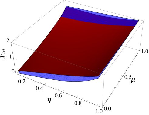
Figure 1: (color online) Lower bounds $\chi_{lwb_{{\cal G}_{1}}}(\eta,\mu)$ (67) (red surface) and $\chi_{lwb_{{\cal G}_{2}}}(\eta,\mu)$ (77) (blue surface). For small $\mu$, $\chi_{lwb_{{\cal G}_{1}}}>\chi_{lwb_{{\cal G}_{2}}}$

In Fig. 2 (top) we plot the populations (63) of the ensemble ${\cal G}_{1}$ (61)-(62) which solves the optimization problem (67). The populations are plotted as functions of the memory degree $\mu$, for two values of the channel transmissivity: $\eta=0.3$ (left plot) and $\eta=0.8$ (right plot). ¿From the numerical optimization it turns out that states of the optimal ensemble (61)-(62) exhibit the same weights for the components $|{01}\rangle$ and $|{10}\rangle$ ($|b|^{2}=|c|^{2}$). Note also that for low values of the channel transmissivity ($\eta=0.3$ in the left plot) and for $\mu\approx 1$, the states (62) have vanishing components along $|{11}\rangle$; indeed for small values of the transmissivity, when $\mu$ approaches 1, the subspace spanned by $\{|{00}\rangle,|{01}\rangle,|{10}\rangle\}$ becomes noiseless, and it is not convenient to use the state $|{11}\rangle$ to encode information. In this last case the bound $\chi_{lwb_{{\cal G}_{1}}}$ is close to $\log_{2}3$. It is worth noting that from numerical analysis it turns out that the maximum (67) is also reached for $\varphi_{1}=\varphi_{2}=\varphi_{3}=0$ (which means that the maximum of the Holevo quantity is reached for real coefficients $a=\bar{a},b=\bar{b},c=\bar{c}$).

In Fig. 2 (bottom panels) we plot the populations of the ensemble ${\cal G}_{2}$ (69)-(74) which solve the optimization (77). It is interesting to notice that for low values of the channel transmissivity ($\eta=0.3$ in the figure), the state $|{11}\rangle$ is not populated for low values of the memory degree, and it is “activated” for a large enough degree of memory. In other words, for $\eta\lesssim 0.6$, we can identify a threshold value $\mu_{th}(\eta)$ below which $|{11}\rangle$ is not populated; it turns out that the smaller is $\eta$, the greater is $\mu_{th}$.

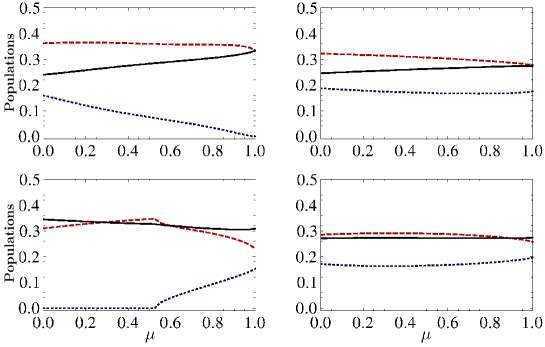
Figure 2: (color online) Populations which maximize the Holevo quantity for the ensemble ${\cal G}_{1}$ (top plots) and for ${\cal G}_{2}$ (bottom plots), at channel transmissivity $\eta=0.3$ (left) and $\eta=0.8$ (right), as functions of the memory degree $\mu$. For the ensemble ${\cal G}_{1}$: $\alpha$ (red long-dashed curve), $\beta=\gamma$ (black full curve), and $\delta$ (blue dashed curve). For the ensemble ${\cal G}_{2}$: $\alpha=(1-2\beta)\cos^{2}\theta_{2}$ (red long-dashed curve), $\beta$ (black full curve), $\delta=(1-2\beta)\sin^{2}\theta_{2}$ (blue dashed curve).

We investigate the amount of entanglement required for the transmission of classical information by considering the average entanglement of the quantum ensemble $\{p_{k},|{\psi_{k}}\rangle\}$ employed, defined as

$$E_{\{p_{k},|{\psi_{k}}\rangle\}}=\sum_{k}p_{k}E(|{\psi_{k}}\rangle),$$ (78)

where $E(|{\psi_{k}}\rangle)$ is the entropy of entanglement HorodeckiReview of the bipartite pure state $|{\psi_{k}}\rangle$. The entanglement related to the ensemble ${\cal G}_{1}$ is simply the entanglement of the state $|{\psi}\rangle$ in (62)

$$E_{{\cal G}_{1}}=E(|{\psi}\rangle),$$ (79)

since all the states (61) have the same entanglement (${\cal R}_{i}$ are local unitary operations, and it is simple to verify that ${\cal S}_{\textrm{w}}$ does not change the entanglement of the pure state $|{\psi}\rangle$). Instead, the average entanglement of the ensemble ${\cal G}_{2}$ (69)-(74) is given by

$$E_{{\cal G}_{2}}\,=\,(1-2\beta)E(|{\phi_{\pm}}\rangle),$$ (80)

since one can always choose separable states inside the subspace spanned by $\{|{01}\rangle,|{10}\rangle\}$ and therefore the states $\{|{\varphi_{\pm}}\rangle\}$ in the ensemble (74) do not contribute to the average entanglement, and the probability of using a state $|{\phi_{\pm}}\rangle$ (74) is $1-2\beta$ (the states $|{\phi_{\pm}}\rangle$ have the same entanglement).

In Fig. 3 we plot both the average entanglement in the ensembles ${\cal G}_{1}$ (black full curve) and ${\cal G}_{2}$ (red dashed curve), for those parameters that solve the optimization problems (67) and (77), respectively. As we can see, in the case of ${\cal G}_{1}$, entanglement is more useful for poor channels (low values of $\eta$). For a given value of the transmissivity, the greater is the memory degree $\mu$ of the channel, the higher is the amount of entanglement associated to the optimal ensemble ${\cal G}_{1}$. In the case of ${\cal G}_{2}$ we find that the presence of entanglement in the ensemble obeys a threshold behaviour. Actually the average entanglement (80) vanishes if the population of the state $|{11}\rangle$ vanishes. For “good” quality channels ($\eta\gtrsim 0.7$), the entanglement associated to the optimal ensembles behaves differently: ${\cal G}_{1}$ exhibits negligible average entanglement for all values of the degree of memory, whereas ${\cal G}_{2}$ requires highly entangled states.

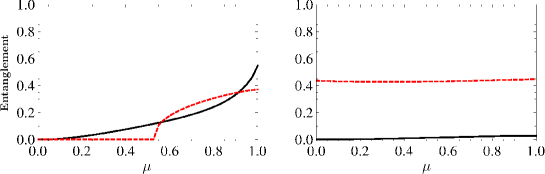
Figure 3: (color online) Average entanglement of the ensembles ${\cal G}_{1}$ (black full curve) and ${\cal G}_{2}$ (red dashed curve), for those parameters which maximize the Holevo quantity, for channel transmittivity $\eta=0.3$ (left) and $\eta=0.8$ (right).

Finally, we want to comment on the $C_{2}$ capacity of a memoryless amplitude damping channel ($\mu=0$). Since the Holevo quantity in general is not additive hastings (and it has not been demonstrated to be additive for the amplitude damping channel), it is worth investigating whether entangled states may be useful to overcome the product state capacity $2\,C_{madc,1}$ (relative to two uses of a memoryless amplitude damping channel), namely whether

$$\max_{\{p_{i},|{\psi_{i}}\rangle\}}\chi\big{(}{\cal E}\otimes{\cal E},\{p_{i},|{\psi_{i}}\rangle\}\big{)}\underbrace{>}_{?}2\,C_{{madc,1}},$$ (81)

where $\{p_{i},|{\psi_{i}}\rangle\}$ is a generic quantum ensemble in the Hilbert space of two qubits, and ${\cal E}$ is the single-qubit amplitude damping channel. The answer to this question requires the optimization in the left member of (81) for any possible ensemble of the form (57, 58), which is a very difficult task. We can, nevertheless investigate the behaviour of the ensembles ${\cal G}_{1}$ and ${\cal G}_{2}$. By numerical analysis it turns out that the maximization of the Holevo quantity over the ensemble ${\cal G}_{2}$ (77) always returns a value smaller than $2\,C_{madc,1}$, while the maximization on the class ${\cal G}_{1}$ (67) returns the value $2\,C_{madc,1}$.

IV Quantum Capacity

In this section we consider the quantum capacity for the amplitude damping channel with memory and derive bounds for it. We recall that the quantum capacity $Q$ is defined as lloyd ; barnum ; devetak

$$Q\,=\,\lim_{n\to\infty}\frac{Q_{n}}{n},\quad\quad Q_{n}\,=\,\max_{\rho^{(n)}}I_{c}(\mathcal{E}_{\mu}^{\otimes n},\rho^{(n)}),$$ (82)

where $\rho^{(n)}$ is an input state for $n$ channel uses and

$$I_{c}(\mathcal{E}_{\mu}^{\otimes n},\rho^{(n)})\,=\,S\big{(}\mathcal{E}_{\mu}^{\otimes n}\big{(}\rho^{(n)}\big{)}\big{)}\,-\,S_{e}(\mathcal{E}_{\mu}^{\otimes n},\rho^{(n)})$$ (83)

is the coherent information schumachernielsen . In Eq. (82) $S_{e}(\mathcal{E}_{\mu}^{\otimes n},\rho^{(n)})$ is the entropy exchange schumacher , defined as

$$S_{e}(\mathcal{E}_{\mu}^{\otimes n},\rho^{(n)})=S\big{[}\big{(}\mathcal{I}\otimes\mathcal{E}_{\mu}^{\otimes n}\big{)}\big{(}|\Psi\rangle\langle\Psi\big{)}\big{]},$$ (84)

where $|\Psi\rangle$ is any purification of $\rho^{(n)}$, namely $\rho^{(n)}=\mathrm{Tr}_{\textsf{R}}|\Psi\rangle\langle\Psi|$ with R denoting a reference system that evolves trivially, according to the identity superoperator $\mathcal{I}$.

In order to calculate the quantum capacity of the memory channel ${\cal E}_{\mu}$ we need to deal with a unitary representation of this channel. This can be conveniently achieved by considering two external systems $E$ and $M$, the latter taking into account the degree of memory of the channel, as follows:

$$|{00}\rangle^{\textsf{S}}\otimes|{00}\rangle^{\textsf{E}}\otimes|{0}\rangle^{\textsf{M}}\quad\longrightarrow$$

$$\hskip 42.67912pt\footnotesize|{00}\rangle^{\textsf{S}}\otimes|{00}\rangle^{\textsf{E}}\otimes\Big{(}\sqrt{1-\mu}|{0}\rangle^{\textsf{M}}+\sqrt{\mu}|{1}\rangle^{\textsf{M}}\Big{)},\normalsize$$

$$|{01}\rangle^{\textsf{S}}\otimes|{00}\rangle^{\textsf{E}}\otimes|{0}\rangle^{\textsf{M}}\quad\longrightarrow\quad\sqrt{1-\mu}\,\Big{(}\sqrt{\eta}|{01}\rangle^{\textsf{S}}\otimes|{00}\rangle^{\textsf{E}}+$$

$$\hskip 42.67912pt\sqrt{1-\eta}|{00}\rangle^{\textsf{S}}\otimes|{01}\rangle^{\textsf{E}}\Big{)}\otimes|{0}\rangle^{\textsf{M}}\,+\,\sqrt{\mu}|{01}\rangle^{\textsf{S}}\otimes|{00}\rangle^{\textsf{E}}\otimes|{1}\rangle^{\textsf{M}},$$

$$|{10}\rangle^{\textsf{S}}\otimes|{00}\rangle^{\textsf{E}}\otimes|{0}\rangle^{\textsf{M}}\quad\longrightarrow\quad\sqrt{1-\mu}\,\Big{(}\sqrt{\eta}|{10}\rangle^{\textsf{S}}\otimes|{00}\rangle^{\textsf{E}}+$$

$$\hskip 42.67912pt\sqrt{1-\eta}|{00}\rangle^{\textsf{S}}\otimes|{10}\rangle^{\textsf{E}}\Big{)}\otimes|{0}\rangle^{\textsf{M}}\,+\,\sqrt{\mu}|{10}\rangle^{\textsf{S}}\otimes|{00}\rangle^{\textsf{E}}\otimes|{1}\rangle^{\textsf{M}},$$

$$|{11}\rangle^{\textsf{S}}\otimes|{00}\rangle^{\textsf{E}}\otimes|{0}\rangle^{\textsf{M}}\quad\longrightarrow$$

$$\hskip 42.67912pt\sqrt{1-\mu}\Big{[}\eta|{11}\rangle^{\textsf{S}}\otimes|{00}\rangle^{\textsf{E}}\,+\,\sqrt{\eta(1-\eta)}\Big{(}|{01}\rangle^{\textsf{S}}\otimes|{10}\rangle^{\textsf{E}}\,+$$

$$\hskip 42.67912pt|{10}\rangle^{\textsf{S}}\otimes|{01}\rangle^{\textsf{E}}\Big{)}\,+\,(1-\eta)|{00}\rangle^{\textsf{S}}\otimes|{11}\rangle^{\textsf{E}}\Big{]}\otimes|{0}\rangle^{\textsf{M}}\,+$$

$$\hskip 42.67912pt\sqrt{\mu}\Big{(}\sqrt{\eta}|{11}\rangle^{\textsf{S}}\otimes|{00}\rangle^{\textsf{E}}\,+\,\sqrt{1-\eta}|{00}\rangle^{\textsf{S}}\otimes|{11}\rangle^{\textsf{E}}\Big{)}\otimes|{1}\rangle^{\textsf{M}}.$$

(85)

When the system S is prepared in the generic pure state $|{\psi}\rangle$ the system SEM state undergoes the transformation

$$|{\psi^{\textsf{SEM}}}\rangle\,=\,|{\psi}\rangle^{\textsf{S}}\otimes|{000}\rangle^{\textsf{EM}}\,=$$

$$\,a|{00}\rangle^{\textsf{S}}\otimes|{000}\rangle^{\textsf{EM}}\,+\,b|{01}\rangle^{\textsf{S}}\otimes|{000}\rangle^{\textsf{EM}}\,+$$

$$+\,c|{10}\rangle^{\textsf{S}}\otimes|{000}\rangle^{\textsf{EM}}\,+\,d|{11}\rangle^{\textsf{S}}\otimes|{000}\rangle^{\textsf{EM}}\qquad\longrightarrow$$

$$|{\psi^{\textsf{SEM}^{\prime}}}\rangle\,=a\sqrt{1-\mu}|{00}\rangle^{\textsf{S}}\otimes|{000}\rangle^{\textsf{EM}}+a\sqrt{\mu}|{00}\rangle^{\textsf{S}}\otimes|{001}\rangle^{\textsf{EM}}+$$

$$\hskip 14.22636ptb\sqrt{(1-\mu)\eta}|{01}\rangle^{\textsf{S}}\!\!\otimes\!\!|{000}\rangle^{\textsf{EM}}+b\sqrt{(1-\mu)(1-\eta)}|{00}\rangle^{\textsf{S}}\!\!\otimes\!\!|{010}\rangle^{\textsf{EM}}+$$

$$\hskip 31.2982ptb\sqrt{\mu}|{01}\rangle^{\textsf{S}}\!\!\otimes\!\!|{001}\rangle^{\textsf{EM}}+$$

$$\hskip 14.22636ptc\sqrt{(1-\mu)\eta}|{10}\rangle^{\textsf{S}}\!\!\otimes\!\!|{000}\rangle^{\textsf{EM}}+c\sqrt{(1-\mu)(1-\eta)}|{00}\rangle^{\textsf{S}}\!\!\otimes\!\!|{100}\rangle^{\textsf{EM}}+$$

$$\hskip 31.2982ptc\sqrt{\mu}|{10}\rangle^{\textsf{S}}\!\!\otimes\!\!|{001}\rangle^{\textsf{EM}}+$$

$$\hskip 14.22636ptd\sqrt{(1-\mu)}\eta|{11}\rangle^{\textsf{S}}\!\!\otimes\!\!|{000}\rangle^{\textsf{EM}}+$$

$$\hskip 31.2982ptd\sqrt{(1-\mu)\eta(1-\eta)}\big{(}|{01}\rangle^{\textsf{S}}\!\!\otimes\!\!|{100}\rangle^{\textsf{EM}}+|{10}\rangle^{\textsf{S}}\!\!\otimes\!\!|{010}\rangle^{\textsf{EM}}\big{)}+$$

$$\hskip 31.2982ptd\sqrt{1-\mu}(1-\eta)|{00}\rangle^{\textsf{S}}\!\!\otimes\!\!|{110}\rangle^{\textsf{EM}}+$$

$$\hskip 31.2982ptd\sqrt{\mu\eta}|{11}\rangle^{\textsf{S}}\!\!\otimes\!\!|{001}\rangle^{\textsf{EM}}+d\sqrt{\mu(1-\eta)}|{00}\rangle^{\textsf{S}}\!\!\otimes\!\!|{111}\rangle^{\textsf{EM}}.$$ (86)

¿From equation (86) it is possible to obtain the expressions for the final state of the system, $\rho^{\prime}={\cal E}_{\mu}(\rho)\equiv\rho^{\textsf{S}^{\prime}}=\textrm{Tr}~{}_{\textsf{EM}}\big{[}|{\psi^{\textsf{SEM}^{\prime}}}\rangle\langle{\psi^{\textsf{SEM}^{\prime}}}|\big{]}$, and of the environment, $\rho^{\textsf{EM}^{\prime}}=\textrm{Tr}~{}_{\textsf{S}}\big{[}|{\psi^{\textsf{SEM}^{\prime}}}\rangle\langle{\psi^{\textsf{SEM}^{\prime}}}|\big{]}$. We report their explicit form in the appendix A.1, see equations (110) and (111).

The two extreme cases of memoryless ($\mu=0$) and full memory ($\mu=1$) amplitude damping channels have been shown to be degradable giovannetti ; MADC2013 , so that the regularization $n\to\infty$ in Eq. (82) is not necessary degradable and the quantum capacity is given by the single-shot formula, $Q=Q_{1}$. On the other hand, there is no evidence that degradability holds for the general case of partial memory. To hand the regularization formula in Eq. (82) is a hard task, therefore we restrict to the computation of upper and lower bounds for the quantum capacity.

IV.1 An upper bound for $Q({\cal E}_{\mu})$

Since the channel ${\cal E}_{\mu}$ is a convex combination of the degradable channels ${\cal E}_{0}$ and ${\cal E}_{m}$, according to Eq. (27), its quantum capacity is upper bounded by smith-smolin07

$$Q_{upb}\,=\,(1-\mu)Q({\cal E}_{0})\,+\,\mu\,Q({\cal E}_{m}).$$ (87)

This expression is easy to evaluate, since $Q({\cal E}_{0})$ is known from Ref giovannetti , and $Q({\cal E}_{m})$ is known from Ref MADC2013 .

IV.2 A lower bound for $Q({\cal E}_{\mu})$

Here we use the “single-letter” formula $Q_{1}$, namely

$$Q_{1}({\cal E}_{\mu})\,=\,\max_{\rho}\,I_{c}({\cal E}_{\mu},\rho),$$ (88)

where $\rho$ belongs to the Hilbert space corresponding to a single use of channel ${\cal E}_{\mu}$. The coherent information is then given by

$$I_{c}({\cal E}_{\mu},\rho)=\,S({\cal E}_{\mu}(\rho))\,-S_{e}({\cal E}_{\mu},\rho)=S(\rho^{\prime})\,-\,S(\rho^{\textsf{EM}^{\prime}}),$$ (89)

where $S_{e}({\cal E}_{\mu},\rho)\,=\,S(\rho^{\textsf{EM}^{\prime}})$ is the entropy exchange related to ${\cal E}_{\mu}$ schumachernielsen .

Since we do not know whether the coherent information of ${\cal E}_{\mu}$ is concave, we cannot simplify the form of the optimal input state by the argument followed in the previous section for the Holevo quantity. As far as we know, the concavity holds for $I_{c}({\cal E}_{\mu},\rho)$ only in the cases $\mu=0,1$. For the generic case of $\mu\neq 0,1$ one should then try to maximize the coherent information (89) with respect to all possible input states $\rho^{\textsf{S}}$. This task is a hard task since it involves a maximization with respect to 15 real parameters. We will then focus on a simpler task, by optimizing the coherent information (89) with respect to a diagonal input state

$$\rho=\left(\begin{array}[]{cccc}\alpha&0&0&0\\ 0&\beta&0&0\\ 0&0&\gamma&0\\ 0&0&0&\delta\\ \end{array}\right).$$ (90)

This choice ensures that for $\mu=0$ and $\mu=1$, the corresponding bound gives the quantum capacity of the memoryless and of the full-memory channel, respectively, since the optimal input is a diagonal one for both channels, as shown in Ref. giovannetti and Ref. MADC2013 . The corresponding output density operators for the system S and the environment ME can be derived from equations (110) and (111), and are shown below:

$$\rho^{\prime}=\left(\begin{array}[]{cccc}\rho^{\textsf{S}^{\prime}}_{00,00}&0&0&0\\ 0&\rho^{\textsf{S}^{\prime}}_{01,01}&0&0\\ 0&0&\rho^{\textsf{S}^{\prime}}_{10,10}&0\\ 0&0&0&\rho^{\textsf{S}^{\prime}}_{11,11}\\ \end{array}\right),$$ (95)

$$\rho^{\textsf{EM}^{\prime}}=\left(\begin{array}[]{cccccccc}\rho^{\textsf{EM}^{\prime}}_{000,000}&\rho^{\textsf{EM}^{\prime}}_{000,001}&0&0&0&0&0&0\\ \rho^{\textsf{EM}^{\prime}}_{001,000}&\rho^{\textsf{EM}^{\prime}}_{001,001}&0&0&0&0&0&0\\ 0&0&\rho^{\textsf{EM}^{\prime}}_{010,010}&0&0&0&0&0\\ 0&0&0&0&0&0&0&0\\ 0&0&0&0&\rho^{\textsf{EM}^{\prime}}_{100,100}&0&0&0\\ 0&0&0&0&0&0&0&0\\ 0&0&0&0&0&0&\rho^{\textsf{EM}^{\prime}}_{110,110}&\rho^{\textsf{EM}^{\prime}}_{110,111}\\ 0&0&0&0&0&0&\rho^{\textsf{EM}^{\prime}}_{111,110}&\rho^{\textsf{EM}^{\prime}}_{111,111}\\ \end{array}\right),$$ (104)

where the matrix elements are reported in the appendix A.1 in Eqs. (110) and (111). Our lower bound for the quantum capacity of the channel ${\cal E}_{\mu}$ is given by

$$Q_{lwb}=\max_{\alpha,\beta,\gamma,\delta}\{I_{c}({\cal E}_{\mu},\rho),0\}\,=\max_{\alpha,\beta,\gamma,\delta}\,\Big{\{}\Big{[}S(\rho^{\prime})\,-\,S(\rho^{\textsf{EM}^{\prime}})\Big{]},0\Big{\}},$$ (105)

whera $\alpha,\beta,\gamma,\delta\in[0,1]$, $\alpha+\beta+\gamma+\delta=1$, $\rho^{\prime}$ and $\rho^{\textsf{EM}^{\prime}}$ are given by (95) and (104), respectively. We solved the optimization problem (105) numerically. The obtained results are reported in the following subsection.

IV.3 Numerical results

In Fig. 4 we plot the bounds (87) and (105) as functions of the memory degree $\mu$, for different values of the transmissivity parameter $\eta$. We first notice that the lower bound (105) exhibits a threshold value $\bar{\mu}_{th}$. Indeed for $\mu\leq\bar{\mu}_{th}$ we have that $Q_{lwb}\,=\,0$. This threshold depends on the channel transmissivity $\eta$, and it is only present for $\eta\leq 0.5$. This is not too surprising, since ${\cal E}_{\mu}$ is a convex combination of two channels and one of them, i.e. the memoryless channel, has a vanishing quantum capacity for $\eta\leq 0.5$. We would like to point out that for $\eta>0.5$ the chosen upper (87) and lower bounds (105) give good estimations of the quantum capacity for ${\cal E}_{\mu}$, since the corresponding values are close to each other, as one can see from Fig. 4.

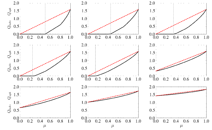
Figure 4: (color online) Upper bound $Q_{upb}$ (87) (red dashed curve) and lower bound $Q_{lwb}$ (105) (black full curve) for the quantum capacity of the channel ${\cal E}_{\mu}$. Different plots refer to different channel transmissivities: from left to right, $\eta=0,0.1,0.2$ (top row), $0.3,0.4,0.6$ (middle row), and $0.7,0.8,0.9$. The dashed gray line signals the presence of a threshold $\bar{\mu}_{th}$: for values of the channel degree of memory $\mu\leq\bar{\mu}_{th}$, the lower bound (105) vanishes.

In Fig. 5 we plot the values of the populations $\alpha,\,\beta,\,\gamma,\,\delta$ (90), which solve the maximization problem (105). We notice that the maximization problem (105) returns equal populations for the states $|{01}\rangle$ and $|{10}\rangle$, $\beta=\gamma$. For low values of transmissivity ($\eta\leq 0.5$) the state $|{11}\rangle$ is not populated. This can be explained by some considerations. First, we notice that the state $|{11}\rangle$ is the one which experiences the strongest noise (greatest damping rates), see the Kraus operators $A_{0}$ in Eqs. (24) and $B_{0}$ in Eqs. (26). Moreover, we remind that the channel ${\cal E}_{\mu}$ is a convex combination of the memoryless channel ${\cal E}_{0}$ and the full memory channel ${\cal E}_{1}$. For $\eta\leq 0.5$, only the channel ${\cal E}_{1}$ has a non vanishing quantum capacity MADC2013 and the optimal ensemble which maximizes the coherent information of ${\cal E}_{1}$ is a diagonal one (90), with vanishing populations $\delta$ (for $\eta\leq 0.5$), as reported in Ref. MADC2013 .

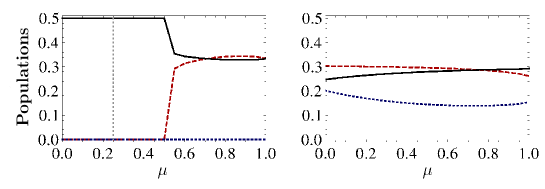
Figure 5: (color online) Populations $\alpha$ (long-dashed red curve), $\beta=\gamma$ (black curve), and $\delta$ (dashed blue curve) which solve the maximization problem (105), for $\eta=0.3$ (left) and $\eta=0.8$ (right). The dashed gray curve signals the presence of a threshold $\bar{\mu}_{th}$: for values of the channel degree of memory $\mu\leq\bar{\mu}_{th}$, the maximum of the coherent information (89) with respect to the input (90) is smaller than or equal to 0.

V Classical Entanglement-Assisted Capacity

In this section we compute the entanglement-assisted classical capacity $C_{E}$, which gives the maximum amount of classical information that can be reliably transmitted down the channel per channel use, provided the sender and the receiver share an infinite amount of prior entanglement. It is given by bennett1999 ; bennett-shor

$$C_{E}\,=\max_{\rho}I(\mathcal{E}_{\mu},\rho),$$ (106)

where the maximization is performed over the input state $\rho$ for a single use of the channel $\mathcal{E}_{\mu}$ and

$$I(\mathcal{E}_{\mu},\rho)\,=S(\rho)+I_{c}(\mathcal{E}_{\mu},\rho).$$ (107)

The subadditivity of $I$ adami-Cerf guarantees that no regularization as in (82) is required to obtain $C_{E}$.

By exploiting the concavity of $I$ adami-Cerf and the covariance properties of the channel, following similar arguments as the ones reported in sect. III.1, we can prove that the state $\rho$ maximizing $I$ is diagonal with the same populations for the states $|{01}\rangle$ and $|{10}\rangle$, as in Eq. (58). Therefore

$$C_{E}=\max_{\alpha,\beta,\delta}I({\cal E}_{\mu},\rho),\,=\max_{\alpha,\beta,\delta}\,[S(\rho^{\textsf{S}})\,+\,S(\rho^{\textsf{S}^{\prime}})\,-\,S(\rho^{\textsf{EM}^{\prime}})\Big{]}.$$ (108)

The numerical results achieved by maximization of the above expression are reported in Fig. 6. As we can see, for any fixed value of $\eta$ the entanglement assisted capacity is an increasing function of the degree of memory. Therefore, memory effects are beneficial to improve the performance of the channel. In particular, for $\eta=0$ we have a qualitative similar behaviour as the classical capacity. Actually, we can see that $C_{E}$ is vanishing in the memoryless case, but it is always nonzero as soon as the channel has some memory, achieving the maximum value 3 for the full memory case.

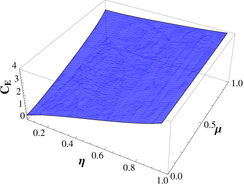
Figure 6: (color online) Entanglement-assisted classical capacity of the channel ${\cal E}_{\mu}$, as a function of the transmittivity $\eta$ and of the degree of memory $\mu$.

In Fig. 7 we plot the populations of the state (58) which solve the maximization problem (108).

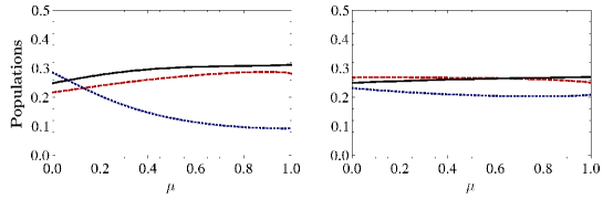
Figure 7: (color online) Coefficients $\alpha$ (red long-dashed curve), $\beta=\gamma$ (black full curve), $\delta$ (blue dashed curve) which solve the maximization problem (108), for $\eta=0.3$ (left) and $\eta=0.8$ (right).

VI Conclusions

In this work we have studied the performance of an amplitude damping channel with memory acting on a two qubits system. We considered a general noise model with arbitrary degree of memory, that includes the memoryless amplitude damping channel and the full memory amplitude damping channel as particular cases. We have analysed three types of scenarios for information transmission. We have first considered the transmission of classical information and have derived lower bounds on the classical channel capacity for a single use of the channel by numerical optimisation of the Holevo quantity for two significant types of input ensembles. We have then considered the case of quantum information and computed upper and lower bounds for the quantum capacity. We emphasized that for high values of the channel transmissivity it turns out that the upper and lower bounds are quite close to each other, thus providing a good estimate of the quantum channel capacity. Finally, we computed the entanglement assisted classical channel capacity numerically for any value of the channel transmissivity $\eta$ and degree of memory $\mu$.

Appendix A Coherent Information for an amplitude damping channel with arbitrary degree of memory

A.1 Expressions for $\rho^{\textsf{S}^{\prime}}$ and $\rho^{\textsf{EM}^{\prime}}$

We describe a generic initial state of the system by the density operator

$$\rho^{\textsf{S}}=\left(\begin{array}[]{cccc}\alpha&\kappa&\lambda&\xi\\ \kappa^{*}&\beta&\nu&o\\ \lambda^{*}&\nu^{*}&\gamma&\pi\\ \xi^{*}&o^{*}&\pi^{*}&\delta\\ \end{array}\right).$$ (109)

The output state of the system S and of the environment EM can be derived from equation (86). We report only the upper triangular part of $\rho^{\textsf{S}^{\prime}}$ and $\rho^{\textsf{EM}^{\prime}}$, since any density operator matrix is an Hermitian matrix.

A.1.1 Matrix $\rho^{\textsf{S}^{\prime}}$

In the basis $\{|{ij}\rangle^{\textsf{S}}\},\,\,i,j\in\{0,1\}$, the $\rho^{\textsf{S}^{\prime}}$ matrix elements are given by (we set $\rho^{\textsf{S}^{\prime}}_{ij,i^{\prime}j^{\prime}}\equiv\,^{\textsf{S}}\!\langle{ij}|\rho^{\textsf{S}^{\prime}}|{i^{\prime}j^{\prime}}\rangle^{\textsf{S}}$)

$$\rho^{\textsf{S}^{\prime}}_{00,00}=(1-\mu)[\alpha+(1-\eta)(\beta+\gamma)+(1-\eta)^{2}\delta]+\mu[\alpha+(1-\eta)\delta],$$

$$\rho^{\textsf{S}^{\prime}}_{00,01}=(1-\mu)[\sqrt{\eta}\kappa+\sqrt{\eta}(1-\eta)\pi]+\mu\kappa,$$

$$\rho^{\textsf{S}^{\prime}}_{00,10}=(1-\mu)[\sqrt{\eta}\lambda+\sqrt{\eta}(1-\eta)o]+\mu\lambda,$$

$$\rho^{\textsf{S}^{\prime}}_{00,11}=[(1-\mu)\,\eta+\mu\,\sqrt{\eta}]\,\xi,$$

$$\rho^{\textsf{S}^{\prime}}_{01,01}=(1-\mu)[\eta\beta+\eta(1-\eta)\delta]+\mu\beta,$$

$$\rho^{\textsf{S}^{\prime}}_{01,10}=[(1-\mu)\,\eta+\mu]\,\nu,$$

$$\rho^{\textsf{S}^{\prime}}_{01,11}=[(1-\mu)\,\eta^{\frac{3}{2}}+\mu\sqrt{\eta}]\,o,$$

$$\rho^{\textsf{S}^{\prime}}_{10,10}=(1-\mu)[\eta\gamma+\eta(1-\eta)\delta]+\mu\gamma,$$

$$\rho^{\textsf{S}^{\prime}}_{10,11}=[(1-\mu)\,\eta^{\frac{3}{2}}+\mu\sqrt{\eta}]\,\pi,$$

$$\rho^{S^{\prime}}_{11,11}=(1-\mu)\eta^{2}\delta+\mu\eta\delta.$$ (110)

A.1.2 Matrix $\rho^{\textsf{EM}^{\prime}}$

The elements of the output environment density matrix $\rho^{\textsf{EM}^{\prime}}$ in the basis $\{|{ijk}\rangle^{\textsf{EM}}\},\,\,i,j,k\in\{0,1\}$, are given by (we set $\rho^{S^{\prime}}_{ijk,i^{\prime}j^{\prime}k^{\prime}}\equiv\,^{\textsf{EM}}\!\langle{ijk}|\rho^{S^{\prime}}|{i^{\prime}j^{\prime}k^{\prime}}\rangle^{\textsf{EM}}$)

$$\rho^{\textsf{EM}^{\prime}}_{000,000}=(1-\mu)\,[\alpha+\eta(\beta+\gamma)+\eta^{2}\delta],$$

$$\rho^{\textsf{EM}^{\prime}}_{000,001}=\sqrt{\mu(1-\mu)}\,[\alpha+\sqrt{\eta}(\beta+\gamma)+\eta^{\frac{3}{2}}\delta],$$

$$\rho^{\textsf{EM}^{\prime}}_{000,010}=(1-\mu)\sqrt{1-\eta}\,(\kappa+\eta\,\pi),$$

$$\rho^{\textsf{EM}^{\prime}}_{000,011}=0,$$

$$\rho^{\textsf{EM}^{\prime}}_{000,100}=(1-\mu)\sqrt{1-\eta}\,(\lambda+\eta\,o),$$

$$\rho^{\textsf{EM}^{\prime}}_{000,101}=0,$$

$$\rho^{\textsf{EM}^{\prime}}_{000,110}=(1-\mu)(1-\eta)\,\xi,$$

$$\rho^{\textsf{EM}^{\prime}}_{000,111}=\sqrt{\mu(1-\mu)(1-\eta)}\,\xi,$$

$$\rho^{\textsf{EM}^{\prime}}_{001,001}=\mu[1-(1-\eta)\delta],$$

$$\rho^{\textsf{EM}^{\prime}}_{001,010}=\sqrt{\mu(1-\mu)(1-\eta)}\,(\kappa+\eta\,\pi),$$

$$\rho^{\textsf{EM}^{\prime}}_{001,011}=0,$$

$$\rho^{\textsf{EM}^{\prime}}_{001,100}=\sqrt{\mu(1-\mu)(1-\eta)}\,(\lambda+\eta\,o),$$

$$\rho^{\textsf{EM}^{\prime}}_{001,101}=0,$$

$$\rho^{\textsf{EM}^{\prime}}_{001,110}=\sqrt{\mu(1-\mu)}(1-\eta)\,\pi,$$

$$\rho^{\textsf{EM}^{\prime}}_{001,111}=\mu\sqrt{1-\eta}\,\pi,$$

$$\rho^{\textsf{EM}^{\prime}}_{010,010}=(1-\mu)(1-\eta)\,(\beta+\eta\,\delta),$$

$$\rho^{\textsf{EM}^{\prime}}_{010,011}=0,$$

$$\rho^{\textsf{EM}^{\prime}}_{010,100}=(1-\mu)(1-\eta)\,\nu,$$

$$\rho^{\textsf{EM}^{\prime}}_{010,101}=0,$$

$$\rho^{\textsf{EM}^{\prime}}_{010,110}=(1-\mu)(1-\eta)^{\frac{3}{2}}\,o,$$

$$\rho^{\textsf{EM}^{\prime}}_{010,111}=\sqrt{\mu(1-\mu)}(1-\eta)\,o,$$

$$\rho^{\textsf{EM}^{\prime}}_{011,ijk}=0\,\quad\forall i,j,k\,\in\{0,1\},$$

$$\rho^{\textsf{EM}^{\prime}}_{100,100}=(1-\mu)(1-\eta)\,(\gamma+\eta\,\delta),$$

$$\rho^{\textsf{EM}^{\prime}}_{100,101}=0,$$

$$\rho^{\textsf{EM}^{\prime}}_{100,110}=(1-\mu)(1-\eta)^{\frac{3}{2}}\,\pi,$$

$$\rho^{\textsf{EM}^{\prime}}_{100,111}=\sqrt{\mu(1-\mu)}(1-\eta)\,\pi,$$

$$\rho^{\textsf{EM}^{\prime}}_{101,ijk}=0\,\quad\forall i,j,k\,\in\{0,1\},$$

$$\rho^{\textsf{EM}^{\prime}}_{110,110}=(1-\mu)(1-\eta)^{2}\delta,$$

$$\rho^{\textsf{EM}^{\prime}}_{110,111}=\sqrt{\mu(1-\mu)}(1-\eta)^{\frac{3}{2}}\,\delta,$$

$$\rho^{\textsf{EM}^{\prime}}_{111,111}=\mu(1-\eta)\delta.$$ (111)

References

• (1) T. M. Cover and J. A. Thomas, Elements of Information Theory (Wiley, New York, 2006).
• (2) M. A. Nielsen and I. L. Chuang, Quantum computation and quantum information (Cambridge University Press, Cambridge, 2000).
• (3) G. Benenti, G. Casati, and G. Strini, Principles of quantum computation and information, vol. II (World Scientific, Singapore, 2007).
• (4) M. M. Wilde, Quantum Information Theory (Cambridge University Press, New York, 2013).
• (5) P. Hausladen, R. Jozsa, B. Schumacher, M. Westmoreland, and W. K. Wootters, Phys. Rev. A 54, 1869 (1996).
• (6) B. Schumacher and M. D. Westmoreland, Phys. Rev. A 56, 131 (1997).
• (7) A. S. Holevo, IEEE Trans. Inf. Theory 44, 269 (1998).
• (8) S. Lloyd, Phys. Rev. A 55, 1613 (1997).
• (9) H. Barnum, M. A. Nielsen, and B. Schumacher, Phys. Rev. A 57, 4153 (1998).
• (10) I. Devetak, IEEE Trans. Inf. Theory 51, 44 (2005).
• (11) C. Adami and N. J. Cerf, Phys. Rev. A 56, 3470 (1997).
• (12) C. H. Bennett, P. W. Shor, J. A. Smolin, and A. V. Thapliyal, Phys. Rev. Lett. 83, 3081 (1999).
• (13) C. H. Bennett, P. W. Shor, J. A. Smolin, and A. V. Thapliyal, IEEE Trans. Inf. Theory 48, 2637 (2002).
• (14) K. Banaszek, A. Dragan, W. Wasilewski, and C. Radzewicz, Phys. Rev. Lett. 92, 257901 (2004).
• (15) Y. Makhlin, G. Schön, and A. Shnirman, Rev. Mod. Phys. 73, 357 (2001); E. Paladino, L. Faoro, G. Falci, and R. Fazio, Phys. Rev. Lett. 88, 228304 (2002); G. Falci, A. D’Arrigo, A. Mastellone, and E. Paladino, Phys. Rev. Lett. 94, 167002 (2005); G. Ithier, E. Collin, P. Joyez, P. J. Meeson, D. Vion, D. Esteve, F. Chiarello, A. Shnirman, Y. Makhlin, J. Schriefl, and G. Schön, Phys. Rev. B 72, 134519 (2005). J. Bylander, S. Gustavsson, F. Yan, F. Yoshihara, K. Harrabi, G. Fitch, D. G. Cory, Y. Nakamura, J.-S. Tsai, W. D. Oliver, Nat. Phys. 7 565 (2011). E. Paladino, Y. M. Galperin, G. Falci, B. L. Altshuler, Rev. Modern Phys. 86, 361 (2014).
• (16) C. Macchiavello and G. M. Palma, Phys. Rev. A 65, 050301(R) (2002).
• (17) L. Memarzadeh, C. Macchiavello and S. Mancini, New J. Phys. 13, 103031 (2011).
• (18) C. Macchiavello, G. M. Palma, and S. Virmani, Phys. Rev. A 69, 010303(R) (2004).
• (19) D. Daems, Phys. Rev. A 76, 012310 (2007).
• (20) Z. Shadman, H. Kampermann, D. Bruss and C. Macchiavello, Phys. Rev. A 84, 042309 (2011); Z. Shadman, H. Kampermann, D. Bruss and C. Macchiavello, Phys. Rev. A 85, 052306 (2012).
• (21) H. Hamada, J. Math. Phys. 43 4382 (2002),
• (22) A. D’Arrigo, G. Benenti, and G. Falci, New J. Phys. 9, 310 (2007).
• (23) M. B. Plenio and S. Virmani, Phys. Rev. Lett. 99, 120504 (2007); New J. Phys. 10, 043032 (2008).
• (24) G. B. Lemos and G. Benenti, Phys. Rev. A 81, 062331 (2010).
• (25) N. Arshed, A. H. Toor, and D. A. Lidar, Phys. Rev. A 81, 062353 (2010).
• (26) N.J. Cerf, J. Clavareau, C. Macchiavello and J. Roland, Phys. Rev. A 72, 042330 (2005).
• (27) O. V. Pilyavets, V. G. Zborovskii, and S.Mancini, Phys. Rev. A 77, 052324 (2008).
• (28) C. Lupo, V. Giovannetti, and S. Mancini, Phys. Rev. Lett. 104, 030501 (2010).
• (29) A. Bayat, D. Burgarth, S. Mancini, and S. Bose, Phys. Rev. A 77, 050306(R) (2008).
• (30) V. Giovannetti and G. M. Palma, Phys. Rev. Lett. 108, 040401 (2012).
• (31) F. Caruso, S. F. Huelga, and M. B. Plenio, Phys. Rev. Lett. 105, 190501 (2010).
• (32) G. Benenti, A. D’Arrigo, and G. Falci, Phys. Rev. Lett. 103, 020502 (2009); A. D’Arrigo, G. Benenti, and G. Falci, Eur. Phys. J. D 66, 147 (2012).
• (33) F. Caruso, V. Giovannetti, C. Lupo, and S. Mancini, Rev. Mod. Phys. 86, 1203 (2014).
• (34) A. D’Arrigo, G. Benenti, G. Falci and C. Macchiavello, Phys. Rev. A 88, 042337 (2013).
• (35) V. Giovannetti and R. Fazio, Phys. Rev. A 71, 032314 (2005).
• (36) M. B. Hastings, Nature Physics 5, 255 (2009).
• (37) Y. Yeo and A. Skeen, Phys. Rev. A 67, 064301 (2003).
• (38) R. Jahangir, N. Arshed, and A. H. Toor, preprint arXiv:1207.5612.
• (39) A. S. Holevo, Probl. Inf. Transm. 9, 177 (1973).
• (40) R. Horodecki, P. Horodecki, M. Horodecki, and K. Horodecki, Rev. Mod. Phys. 81, 865 (2009).
• (41) B. W. Schumacher and M. A. Nielsen, Phys. Rev. A 54, 2629 (1996).
• (42) B. W. Schumacher, Phys. Rev. A 54, 2614 (1996).
• (43) I. Devetak and P. W. Shor, Comm. Math. Phys. 256, 287 (2005).
• (44) G. Smith and J. A. Smolin, Additive extensions of a quantum channel, Proceedings of the IEEE Information Theory Workshop 2008 pp 368-372.