Finite-volume effects in the hadronic vacuum polarization

Abstract:

We investigate finite-volume effects in the hadronic vacuum polarization, with an eye toward the corresponding systematic error in the muon anomalous magnetic moment. While it is well known that leading-order chiral perturbation theory does not provide a good description of the hadronic vacuum polarization, it turns out that it gives a much better representation of finite-volume effects. Indications are that finite-volume effects cannot be ignored when the aim is a few percent level accuracy for the hadronic contribution to the muon anomalous magnetic moment, even when $m_{\pi}L\sim 4$ and $m_{\pi}\sim 200$ MeV.

1 Introduction

The leading-order hadronic contribution to the muon anomalous magnetic moment $g=2(1+a_{\mu})$ is given by the expression

$$a^{\rm HVP}_{\mu}=\left(\frac{\alpha}{\pi}\right)^{2}\int_{0}^{\infty}dQ^{2}\,f(Q^{2})\,[\Pi(Q^{2})-\Pi(0)]\ ,$$ (1)

in which $f(Q^{2})$ is a known weight function which depends on the muon mass, and $\Pi(Q^{2})$ is defined by

$$\Pi_{\mu\nu}(Q)=\left(\delta_{\mu\nu}Q^{2}-Q_{\mu}Q_{\nu}\right)\Pi(Q^{2})\ ,$$ (2)

the (euclidean) hadronic vacuum polarization [1, 2]. The integrand of Eq. (1) is peaked around $Q^{2}\sim m_{\mu}^{2}/4$, and shown in Fig. 1.

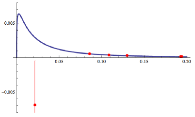
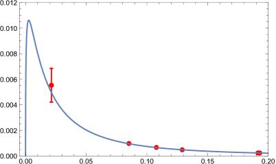
Figure 1: Typical fits (blue curves) to lattice data (red points) for the hadronic vacuum polarization. The figure on the left shows data with statistics typical of 2012 [3], the figure on the right shows data with statistics typical of 2015 (unpublished).

The figure on the right (which was obtained with AMA improvement [4]) shows that dramatic improvement with statistics was made over the last few years. But the figures also show that $a^{\rm HVP}_{\mu}$ is very sensitive to the very-low $Q^{2}$ region. Thus, in addition to the need for more data with smaller errors at low $Q^{2}$, it is also important to understand systematic effects in detail. Very small changes in $\Pi(Q^{2})$ at low $Q^{2}$ can have dramatic effects on the value of $a^{\rm HVP}_{\mu}$. Here, we will consider the impact of finite-volume effects on $a^{\rm HVP}_{\mu}$, for the case of a volume $L^{3}\times T$, with periodic boundary conditions, $L$ the spatial extent, and $T$ the temporal extent, with $L\neq T$.

2 Theoretical considerations

A first observation is that in finite volume, the Ward–Takahashi identity does not exclude that $\Pi_{\mu\nu}(0)$ does not vanish, because of the discrete nature of momenta in a finite volume. Furthermore, it is reasonable to expect that the hadronic vacuum polarization, with its $\log{Q^{2}}$ behavior, is more singular for low momenta in a finite volume than in infinite volume. This suggests subtracting $\Pi_{\mu\nu}(0)$ from the vacuum polarization at non-zero $Q$. We thus define

$$\overline{\Pi}_{\mu\nu}(Q) \equiv P^{T}_{\mu\kappa}(Q)\left(\Pi_{\kappa\lambda}(Q)-\Pi_{\kappa\lambda}(0)\right)P^{T}_{\lambda\nu}(Q)\ ,$$ (3)

$$P^{T}_{\mu\nu}(Q) = \delta_{\mu\nu}-\frac{Q_{\mu}Q_{\nu}}{Q^{2}}\ .$$

We chose to project the subtracted vacuum polarization so that it satisfies the Ward–Takahashi identity, but this turns out not to be essential in what follows.

This idea has been considered before. For instance, in Ref. [6] a study was made of the effect of this subtraction at different values of the volume; Fig. 2 shows some of the results.

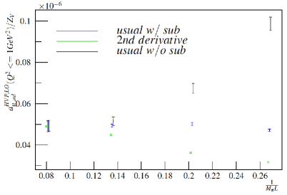
Figure 2: Dependence on volume of $a^{\rm HVP}_{\mu}$, from Ref. [6]. The black points have been obtained without the subtraction of $\Pi_{\mu\nu}(0)$, the blue points with such a subtraction. These data have $a=0.104$ fm, $m_{\pi}=292$ MeV, and $3.7\leq m_{\pi}L\leq 12.3$. For more details, see Ref. [6].

It is clear that the subtraction reduces finite-volume effects significantly, at least for the choice of parameters that were used in Fig. 2.

On the lattice, rotational symmetry is broken by both the lattice itself, and by the shape of the finite volume. When rotational symmetry is broken, the Ward–Takahashi identity allows for tensor structures other than $Q^{2}\delta_{\mu\nu}$ and $Q_{\mu}Q_{\nu}$ in $\Pi_{\mu\nu}(Q)$, such as for instance $\delta_{\mu\nu}\sum_{\kappa}Q^{4}_{\kappa}$ and $Q^{3}_{\mu}Q_{\nu}+Q_{\mu}Q^{3}_{\nu}$. However, because of dimensions, such terms have to appear with coefficients with mass dimension $-2$. That implies that the coefficients have to contain a power $a^{2}$, because the other scales in the theory such as $L$ and $m_{\pi}$ would have to appear as $L^{2}$ or $m_{\pi}^{-2}$, which is clearly impossible. Since we are interested in the low-$Q^{2}$ region, we will assume that, for such momenta, scaling violations can be ignored. It follows that $\overline{\Pi}_{\mu\nu}(Q)$ has to be of the form (2), with the proviso that, since the unbroken group of rotations are just the spatial cubic rotations by 90 degrees, there is more than one irreducible representation (irrep) of the cubic group hiding in this decomposition. In particular, we may project onto the irreps

$$A_{1}:\qquad \sum_{i}\Pi_{ii}\quad\mbox{and}\quad\Pi_{44}\ ,$$ (4)

$$T_{1}:\qquad \Pi_{4i}=\Pi_{i4}\ ,$$

$$T_{2}:\qquad \Pi_{i\neq j}=\Pi_{j\neq i}\ ,$$

$$E:\qquad \Pi_{11}-\sum_{i}\Pi_{ii}/3\ ,\Pi_{22}-\sum_{i}\Pi_{ii}/3\ ,$$

and extract a scalar function $\Pi(Q^{2})$ from each of these. Since cubic rotations do not transform the five different irreps into each other, these scalar functions do not have to be equal. They only become equal to each other in the limit $L,\ T\to\infty$. We will label these five different scalar functions as $\Pi_{A_{1}}$ (from $\sum_{i}\Pi_{ii}$), $\Pi_{A_{1}^{44}}$ (from $\Pi_{44}$), $\Pi_{T_{1}}$, $\Pi_{T_{2}}$ and $\Pi_{E}$.

Assuming that finite-volume effects are dominated by pions, one may also study them in chiral perturbation theory (ChPT). To leading order in ChPT, the hadronic vacuum polarization due to pions in a finite periodic volume $L^{3}\times T$ is given by

$$\Pi^{\rm ChPT}_{\mu\nu}(Q)=\frac{5}{9}e^{2}\Bigg{(}4\,\frac{1}{L^{3}T}\sum_{p}\frac{\sin{\left(p+Q/2\right)_{\mu}}\sin{\left(p+Q/2\right)_{\nu}}}{\left(2\sum_{\kappa}(1-\cos{p_{\kappa}})+m_{\pi}^{2}\right)\left(2\sum_{\kappa}(1-\cos{(p+Q)_{\kappa}})+m_{\pi}^{2}\right)}$$ (5)

$$-2\,\delta_{\mu\nu}\,\frac{1}{L^{3}T}\sum_{p}\left(\frac{\cos{p_{\mu}}}{\left(2\sum_{\kappa}(1-\cos{p_{\kappa})}+m_{\pi}^{2}\right)}\right)\Biggr{)}\ ,$$

where $e$ is the electric charge of the electron, and the sums are over quantized momenta $p_{\mu}=2\pi n_{\mu}/L_{\mu}$, with $n_{\mu}$ integers, and $L_{1}=L_{2}=L_{3}=L$ and $L_{4}=T$. One can show explicitly from this expression that $\Pi^{\rm ChPT}_{\mu\nu}(0)$ does not vanish, but rather, that it is exponentially suppressed with $m_{\pi}L$. In our explorations below, we will compute $\Pi^{\rm ChPT}_{\mu\nu}(Q)$ omitting the factor $5e^{2}/9$.

It is rather well known that leading-order ChPT does not give a good description of vector and axial-vector two-point functions already for very small values of $Q^{2}$. The intuitive reason for this is that the $\rho$ and $a_{1}$ resonances make significant contributions to these two-point functions, whereas leading-order ChPT only sees the pions (vector resonances contribute only through low-energy constants at higher order). However, here we are only interested in the difference between the vacuum polarization in finite and infinite volume. Since for large enough values of $m_{\pi}L$ these differences are exponentially small in the ratio of the linear volume and hadronic Compton wave lengths, it is reasonable to assume that these differences are dominated by pions, and thus well described by leading-order ChPT. We will investigate this in what follows.

3 Comparison between lattice data and theory

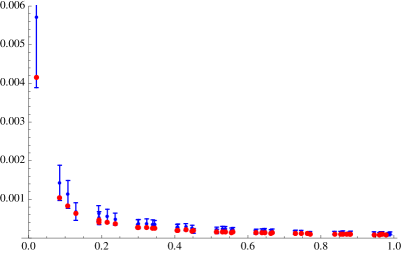
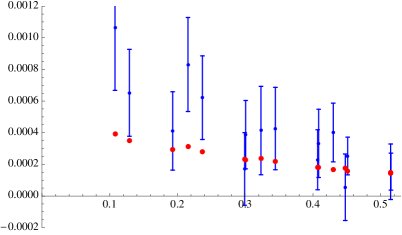
Figure 3: Left panel: difference between the subtracted ($\overline{\Pi}_{A_{1}}(Q^{2})$) and unsubtracted ($\Pi_{A_{1}}(Q^{2})$) $A_{1}$ vacuum polarizations. Right panel: difference between the subtracted ($\overline{\Pi}_{A_{1}}(Q^{2})$) and unsubtracted ($\Pi_{A_{1}^{44}}(Q^{2})$) $A_{1}^{44}$ vacuum polarizations. Red points are computed in ChPT; blue points are lattice data.

Figure 3 shows a comparison between ChPT, using Eq. (5), and lattice data. The lattice points were computed using the MILC asqtad ensemble with $1/a=3.34532$ GeV, $m_{\pi}=220$ MeV, $L=64a$ and $T=144a$, which implies $m_{\pi}L=4.2$. We find that the subtraction of $\Pi_{\mu\nu}(0)$ only makes a significant difference for $\Pi_{A_{1}}$ (as one might expect). The left panel shows the effect of the subtraction itself, while the right panel shows the difference between two different irreps. We see that there is good agreement between ChPT and lattice data, implying that leading-order ChPT does a reasonably good job of describing finite-volume effects. Similar results are obtained for differences between other irreps. Another important conclusion is that the lattice data are precise enough to be able to discern finite-volume effects, thanks to the use of all-mode averaging [4], which was employed to get the data shown. To illustrate this observation, we show in Fig. 4 the lattice data points for $\overline{\Pi}_{A_{1}}(Q^{2})$ and $\Pi_{A_{1}^{44}}(Q^{2})$.

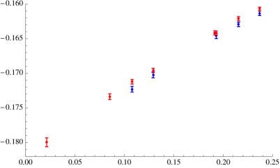
Figure 4: Lattice data for $\overline{\Pi}_{A_{1}}(Q^{2})$ and $\Pi_{A_{1}^{44}}(Q^{2})$.

In Fig. 5, we compare ChPT results for the $A_{1}$, $A_{1}^{44}$ and infinite-volume vacuum polarizations, with the unsubtracted $A_{1}$ case on the left, and the subtracted $A_{1}$ case on the right. Infinite-volume points were computed by replacing $L\to 2L$ and $T\to 2T$ in Eq. (5). As mentioned before, there is very little difference between the subtracted and unsubtracted values for $\Pi_{A_{1}^{44}}(Q^{2})$, and similar plots for the irreps $T_{1,2}$ and $E$ look very similar. As one sees by comparing the left and right panels, the effect of the subtraction for the $A_{1}$ irrep is dramatic at the lowest values of $Q^{2}$, and the subtraction brings $\Pi_{A_{1}}(Q^{2})$ much closer to the infinite-volume result. Thus, ChPT provides a theoretical explanation of this effect. Moreover, it is interesting that after the subtraction, the $A_{1}$ and $A_{1}^{44}$ vacuum polarizations straddle the infinite-volume result. The same thing happens if we replace $A_{1}^{44}$ by any of the other irreps $T_{1,2}$ and $E$.

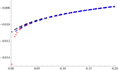
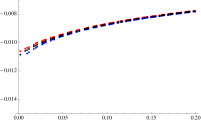
Figure 5: Left panel: ChPT computation of (unsubtracted) $\Pi_{A_{1}}(Q^{2})$ (red points), (unsubtracted) $\Pi_{A_{1}^{44}}(Q^{2})$ (blue points) and the “infinite-volume” result (black points). Right panel: ChPT computation of (subtracted) $\overline{\Pi}_{A_{1}}(Q^{2})$ (red points), (unsubtracted) $\Pi_{A_{1}^{44}}(Q^{2})$ (blue points) and the “infinite-volume” result (black points).

4 Effects on $a_{\mu}^{\rm HVP}$

We now consider what the small, but significant finite-volume effects in $\Pi(Q^{2})$ imply for $a_{\mu}^{\rm HVP}$. We define

$$a^{\rm HVP}_{\mu}(Q^{2}_{max})=\left(\frac{\alpha}{\pi}\right)^{2}\int_{0}^{Q^{2}_{max}}dQ^{2}\,f(Q^{2})\,[\Pi(Q^{2})-\Pi(0)]\ ,$$ (6)

differing from $a^{\rm HVP}_{\mu}$ because of the choice of upper limit of the integral. Below we will choose $Q^{2}_{max}=1$ GeV², to diminish the effect of different systematic errors at large momenta. Close to 100% of the light-quark contribution to $a^{\rm HVP}_{\mu}$ comes from the region below $Q^{2}=1$ GeV² [9].

We first consider $[0,1]$ Padé fits [3] on the interval below 1 GeV², using the $A_{1}$ or $A_{1}^{44}$ data points only. We find

$$a^{\rm HVP}_{\mu,A_{1}}(1~{}\mbox{GeV}^{2}) = 8.4(4)\times 10^{-8}\ ,$$ (7)

$$a^{\rm HVP}_{\mu,A_{1}^{44}}(1~{}\mbox{GeV}^{2}) = 9.2(3)\times 10^{-8}\ .$$

Using instead a quadratic conformally-mapped polynomial [9], we find

$$a^{\rm HVP}_{\mu,A_{1}}(1~{}\mbox{GeV}^{2}) = 8.4(5)\times 10^{-8}\ ,$$ (8)

$$a^{\rm HVP}_{\mu,A_{1}^{44}}(1~{}\mbox{GeV}^{2}) = 9.6(4)\times 10^{-8}\ .$$

While one may argue that these fit functions are not adequate to reach the desired sub-percent level accuracy, the point here is that the Padé and conformally-mapped polynomial fits give results that are consistent within errors (of order 4%). The difference between the $A_{1}$ and $A_{1}^{44}$ fits, however, is about 9–13% larger than the errors shown in Eqs. (7,8), and consistent between the two types of fits. Since the only difference is the irrep onto which we projected the lattice data, we conclude that the 9–13% difference is a finite-volume effect. A phenomenological analysis of finite-volume effects found values consistent with our estimate [10].

5 Conclusion

It is difficult to perform a lattice computation of $a^{\rm HVP}_{\mu}$ with sub-percent level accuracy because of the nature of the integrand in the integral defining this quantity, as demonstrated in Fig. 1. The integrand is strongly peaked at $Q^{2}\approx m_{\mu}^{2}/4$, values of the momenta which are hard to reach on the lattice. Consequently, even small variations of the vacuum polarization itself, due to systematic errors, get magnified to be large variations on $a^{\rm HVP}_{\mu}$. In this talk, we demonstrated that this is also true for the systematic error due to the use of a finite volume.

Together with the conclusions reached in Refs. [3, 9, 11], the picture that emerges is that for good control of the systematic errors, one needs a series of model-independent fit functions to the lattice data for $\Pi(Q^{2})$, approximately physical pion masses, and control over finite-volume effects.

Finally, we note that finite-volume effects are equally likely to affect other methods to construct smooth interpolations of the lattice data for $\Pi(Q^{2})$, such as the moment method proposed in Ref. [12]. In particular, in a finite volume, the $t^{2}$ moment of the vector current correlator is not equal to $\Pi(0)$, but instead to a linear combination of values at non-zero momenta [13]:

$$\Pi(0)\to\sum_{n\neq 0}4(-1)^{n}\Pi\left(\frac{2\pi n}{T}\right)\ .$$ (9)

We do not know of any argument that this linear combination of values of $\Pi(Q^{2})$ is less sensitive to finite-volume effects than any of these values alone.

Acknowledgments We thank Taku Izubuchi and Kim Maltman for useful discussions. TB, PC, MG and CT were supported in part by the US Dept. of Energy; SP by CICYT-FEDER-FPA2014-55613-P, 2014 SGR 1450, the Spanish Consolider-Ingenio 2010 Program CPAN (CSD2007-00042).

References

- [1] T. Blum, Phys. Rev. Lett. 91, 052001 (2003) [hep-lat/0212018].
- [2] B. E. Lautrup, A. Peterman and E. de Rafael, Phys. Rept. 3, 193 (1972).
- [3] C. Aubin, T. Blum, M. Golterman and S. Peris, Phys. Rev. D 86, 054509 (2012) [arXiv:1205.3695 [hep-lat]].
- [4] T. Blum, T. Izubuchi and E. Shintani, Phys. Rev. D 88, no. 9, 094503 (2013) [arXiv:1208.4349 [hep-lat]].
- [5] D. Bernecker and H. B. Meyer, Eur. Phys. J. A 47, 148 (2011) [arXiv:1107.4388 [hep-lat]].
- [6] R. Malak et al. [Budapest-Marseille-Wuppertal Collaboration], PoS LATTICE 2014, 161 (2015) [arXiv:1502.02172 [hep-lat]].
- [7] C. Aubin and T. Blum, Phys. Rev. D 75, 114502 (2007) [hep-lat/0608011].
- [8] D. Boito, M. Golterman, M. Jamin, K. Maltman and S. Peris, Phys. Rev. D 87, no. 9, 094008 (2013) [arXiv:1212.4471 [hep-ph]].
- [9] M. Golterman, K. Maltman and S. Peris, Phys. Rev. D 90, no. 7, 074508 (2014) [arXiv:1405.2389 [hep-lat]].
- [10] A. Francis, B. Jaeger, H. B. Meyer and H. Wittig, Phys. Rev. D 88, 054502 (2013) [arXiv:1306.2532 [hep-lat]].
- [11] M. Golterman, K. Maltman and S. Peris, Phys. Rev. D 88, no. 11, 114508 (2013) [arXiv:1309.2153 [hep-lat]].
- [12] B. Chakraborty et al. [HPQCD Collaboration], Phys. Rev. D 89, no. 11, 114501 (2014) [arXiv:1403.1778 [hep-lat]].
- [13] T. Blum and T. Izubuchi, private notes (2015).