Path Integral approach to nonequilibrium potentials in multiplicative Langevin dynamics

Abstract

We present a path integral formalism to compute potentials for nonequilibrium steady states, reached by a multiplicative stochastic dynamics. We develop a weak-noise expansion, which allows the explicit evaluation of the potential in arbitrary dimensions and for any stochastic prescription. We apply this general formalism to study noise-induced phase transitions. We focus on a class of multiplicative stochastic lattice models and compute the steady state phase diagram in terms of the noise intensity and the lattice coupling. We obtain, under appropriate conditions, an ordered phase induced by noise. By computing entropy production, we show that microscopic irreversibility is a necessary condition to develop noise-induced phase transitions. This property of the nonequilibrium stationary state has no relation with the initial stages of the dynamical evolution, in contrast with previous interpretations, based on the short-time evolution of the order parameter.

1 Introduction

Nonequilibrium statistical mechanics is at the stem of important physical phenomena, many of them at the border with other sciences such as biology, chemistry, geology and even social sciences. Differently from equilibrium statistical mechanics, there is no closed theoretical framework to deal with out-of-equilibrium systems, being the theory of stochastic processes [1] one of the natural approaches to describe them. These systems have been traditionally modeled by stochastic differential equations, as well as through Fokker-Planck equations. Moreover, functional path integral approaches have also been introduced [2]. The latter approach is more adaptive to explore symmetries and general formal aspects of stochastic dynamics, such as out-of-equilibrium fluctuations theorems [3, 4, 5].

Recently, clear advances in the path integral approach of multiplicative processes were made [6, 7, 8, 9]. Multiplicative noise naturally describes inhomogeneous diffusion in which fluctuations depend on the state of the system. Concrete applications are very diverse, covering a broad range of interest as, for instance, micromagnetism [10] and early life biology [11]. On the other hand, extended multiplicative systems present challenging phenomena, such as noise-induced phase transitions (NIPT), stochastic resonance and pattern formation [12, 13]. Although it is possible to define order parameters and susceptibilities in nonequilibrium steady states, the classification of phase transitions in universality classes is still underdeveloped. In fact, a complete general theory of the nonequilibrium Renormalization Group is still lacking. The definition and evaluation of thermodynamical potentials, such as the Helmholtz or Gibbs free energies, are not completely developed in out-of-equilibrium statistical mechanics. Indeed, there is an actual discussion about the possibility of having a thermodynamic description of nonequilibrium steady states [14], although some steps forward for particular systems have been achieved [15, 16, 17, 18, 19, 20].

The main goal of this letter is to provide a general formalism to compute potentials for describing nonequilibrium stationary states reached by a multiplicative Langevin dynamics. Based on a recently introduced path integral formalism [9], we present nonequilibrium generating functionals, appropriated to compute order parameter correlations. We also introduce a systematic and controlled non-perturbative weak-noise approximation to compute these potentials.

We explicitly compute, in the Gaussian fluctuation approximation, the nonequilibrium potential for a wide class of Langevin dynamics, in arbitrary spatial dimensions and for any stochastic prescription, including Itô, Stratonovich and anti-Itô prescriptions. This last point is essential in the study of entropy production and fluctuation theorems, since time-reversal transformations generally mix different prescriptions [8]. As a concrete example, we apply the formalism to a set of models, including the simplest lattice model proposed by Van den Broeck, Parrondo and Toral (VPT) [21] and a related continuum model of Genovese, Muñoz and Sancho [22]. We show that our approximation procedure correctly captures the physics of NIPT and, differently from equilibrium phase transitions, we establish a deep connection between NIPT and microscopic irreversibility [23].

2 Dynamical generating functionals

We begin by considering a system of Langevin equations given by

$$\frac{dx_{i}(t)}{dt}=f_{i}({\bf x}(t))+g_{ij}({\bf x}(t))\eta_{j}(t)\;,$$ (1)

where $i=1,\ldots,n$, $j=1,\ldots,m$, ${\bf x}\in\Re^{n}$ and $\eta_{j}(t)$ are $m$ independent Gaussian white noises: $\left\langle\eta_{i}(t)\right\rangle=0$, $\left\langle\eta_{i}(t),\eta_{j}(t^{\prime})\right\rangle=\sigma^{2}\delta_{ij}\delta(t-t^{\prime})$, where $\sigma^{2}$ measures the noise intensity. We use bold face characters for vector variables and summation over repeated indices is understood. The drift force $f_{i}({\bf x})$ and the diffusion matrix $g_{ij}({\bf x})$ are, in principle, arbitrary smooth functions of ${\bf x}(t)$. Along this letter, we use the Generalized Stratonovich prescription, parametrized by a real number $0\leq\alpha\leq 1$ [8]. Time correlation functions can be computed by performing functional derivatives of a generating functional written in terms of functional integrals. Functional integral techniques in different discretization prescriptions have been developed in Refs. [24, 25, 26]. We have used a generalization of the Martin-Siggia-Rose-Janssen-deDominicis formalism [27, 28, 29], that we have recently implemented [9] to deal with the multi-variable dynamics of Eq. (1) in the $\alpha$-prescription. The generating functional can be written, after integrating out auxiliary variables, in terms of a functional integral over the vector variable ${\bf x}(t)$,

$$Z[{\bf J}]=\int{\cal D}{\bf x}\;{\det}^{-1}(g)\;e^{-\frac{1}{\sigma^{2}}\left\{S[{\bf x}]-\int_{-\infty}^{\infty}dt^{\prime}{\bf J}\cdot{\bf x}(t^{\prime})\right\}}\;,$$ (2)

where the “action” is given by

$$S=\int_{t_{i}}^{t_{f}}\!\!dt\;\left\{\frac{1}{2}\left[\dot{x}_{\ell}-\Gamma_{\ell}\right][g^{2}]^{-1}_{\ell m}\left[\dot{x}_{m}-\Gamma_{m}\right]+\alpha\sigma^{2}\partial_{k}f_{k}\right.$$

$$+ \left.\frac{1}{2}\alpha^{2}\sigma^{2}\left[\partial_{m}g_{kj}(x)\partial_{k}g_{mj}(x)-\partial_{m}g_{mj}(x)\partial_{i}g_{ij}(x)\right]\right\},$$

with $\Gamma_{\ell}({\bf x})=f_{\ell}({\bf x})-\alpha\sigma^{2}g_{\ell j}({\bf x})\partial_{i}g_{ij}({\bf x})$. The second and third terms of Eq. (2), proportional to $\alpha$ and $\alpha^{2}$ respectively, comes from the non-trivial Jacobian associated with the change of variables $\eta_{i}(t)\to x_{i}(t)$. These terms, together with $\alpha-$calculus rules [30] are essential to implement any consistent approximation procedure. In Eq. (2), ${\bf J}(t)$ is a vectorial source necessary to compute correlation functions.

Formally, $Z[{\bf J}(t)]$ plays the same role as the partition function in equilibrium statistical mechanics. Then, it is immediate to define the functional $F[{\bf J}(t)]=-\sigma^{2}\ln Z[{\bf J}]$, from which we can compute a “local order parameter”

$$M_{i}(t)\equiv\langle x_{i}(t)\rangle=-\frac{\delta F[{\bf J}]}{\delta J_{i}(t)}\;.$$ (4)

The dynamical variable ${\bf M}(t)$, in principle, is not an order parameter. However, as we will show below, the homogeneous long-time limit behaves like an actual order parameter, detecting order-disorder phase transitions.

In order to define a generating functional in terms of the order parameter, we perform a Legendre transformation in the following way,

$$G[{\bf M}(t)]=\int dt\;{\bf J}(t)\cdot{\bf M}(t)+F[{\bf J}(t)]\;,$$ (5)

where ${\bf J}(t)\equiv{\bf J}[{\bf M}(t)]$ is defined by inverting Eq. (4). It is immediate to verify $\delta G[{\bf M}]/\delta M_{i}(t)=J_{i}(t)$, that can be interpreted as the nonequilibrium state equation.

Assuming that, at long times, the system reaches an homogeneous stationary state, we can define the nonequilibrium potential as

$$G_{\rm st}(M)=\lim_{t\to\infty}\lim_{N\to\infty}\frac{1}{N}G[{\bf M}(t)]\;,$$ (6)

where $N$ is the number of degrees of freedom and the order parameter $M=(1/N)\lim_{t\to\infty}\sum_{i=1}^{N}\langle x_{i}(t)\rangle$.

The expressions in Eqs. (5) and (6) are the main proposals of this letter. The potential $G_{\rm st}(M)$ is the analog of the Gibbs free energy for describing nonequilibrium stationary states. The critical behavior of the nonequilibrium state is codified in the analytical properties of $G_{\rm st}(M)$.

3 Weak noise expansion

Due to the factor $1/\sigma^{2}$ in the exponential of Eq. (2), the functional integral can be computed in the saddle-point plus Gaussian fluctuations approximation, for small $\sigma$. Assuming there is only one trajectory $x^{0}_{i}(t)$ that extremize the action, we decompose the integration variables as,

$$x_{i}(t)=x^{0}_{i}(t)+\delta x_{i}(t)\;,$$ (7)

where $x^{0}_{i}(t)$ is a solution of

$$\left.\frac{\delta S[{\bf x}]}{\delta x_{i}(t)}\right|_{{\bf x}(t)={\bf x}^{0}}=J_{i}(t)$$ (8)

and $\delta x_{i}(t)$ represent small fluctuations. Replacing Eq. (7) into Eq. (2) and expanding in powers of $\delta x_{i}(t)$ up to quadratic order, we find, after the Gaussian integration,

$$F[{\bf J}]=S[{\bf x}^{0}]-\int dt\;{\bf J}\cdot{\bf x}^{o}+\frac{\sigma^{2}}{2}{\rm Tr}{\ln}[{\bf S}^{(2)}]+\ldots\;,$$ (9)

where the components of the fluctuation matrix ${\bf S}^{(2)}$ are given by

$$S^{(2)}_{ij}(t,t^{\prime})=\frac{\delta^{2}S[{\bf x}]}{\delta x_{i}(t)\delta x_{j}(t^{\prime})}\Bigg{|}_{{\bf{\bf x}(t)}={\bf x}^{0}(t)},$$ (10)

and the ellipsis represents order $\sigma^{4}$ terms. Using Eqs. (4) and (9), we find for the order parameter,

$$M_{i}(t)=x^{0}_{i}(t)-\frac{\sigma^{2}}{2}{\rm Tr}\left\{[{\bf S}^{(2)}]^{-1}\frac{\delta{\bf S}^{(2)}}{\delta J_{i}(t)}\right\}.$$ (11)

For $\sigma\to 0$, the order parameter is essentially the “classical” solution ${\bf M}(t)={\bf x}^{0}(t)$, obtained by solving Eq. (8). Fluctuations change this result in a non-trivial way. To compute the Legendre transformation of Eq. (5), we invert Eq. (11) perturbatively in powers of $\sigma^{2}$. Retaining the leading order terms, we find the expression

$$G[{\bf M}(t)]=S[{\bf M}(t)]+\frac{\sigma^{2}}{2}{\rm Tr}\ln\left\{{\bf S}^{(2)}[{\bf M}(t)]\right\}\;.$$ (12)

Eq. (12) is the explicit expression of the generating functional of the local order parameter in the Gaussian fluctuations approximation. This general result allows the computation of the time-dependent order parameter by solving the dynamical set of equations $\delta G[{\bf M}]/\delta M_{i}(t)=0$, with $i=1,\ldots,N$. At this point, it is important to stress that Eq. (12) was computed assuming that there is only one path $x_{0}(t)$ which solves Eq. (8). In the case of multiple solutions, the method should be generalized by computing Gaussian fluctuations around each solution and summing up each contribution [2].

4 Lattice models

Let us compute $G[{\bf M}(t)]$ for a model consisting in a set of $N$ stochastic variables whose dynamics are driven by the same drift $f(x)$ and the same diffusion function $g(x)$. Each degree of freedom is arranged in a $d$-dimensional hypercubic lattice and we consider short-range lattice couplings. Then, in Eq. (1), we will take $f_{i}({\bf x})=f(x_{i})+F_{i}({\bf x})$ and $g_{ij}({\bf x})=g(x_{i})\delta_{ij}$, where $F_{i}({\bf x})$ represent the lattice couplings. In the absence of couplings, $F_{i}({\bf x})=0$, the system converges, at long times, to an equilibrium state. Imposing the Einstein relation $f(x)=-(1/2)g(x)^{2}dV(x)/dx$, where $V(x)$ is a classical potential, the equilibrium distribution is $P_{\rm eq}\sim\exp\{-(1/\sigma^{2})U_{\rm eq}(x)\}$, with the potential $U_{\rm eq}(x)=V(x)+(1-\alpha)\ln g^{2}(x)$ [8]. The equilibrium potential depends on the stochastic prescription $\alpha$ and, in general, it is not of the Boltzmann type, except for $\alpha=1$. Considering even potentials, $V(x)=V(-x)$, with a single minimum at $x=0$ and $g^{\prime\prime}(0)>0$, we have $\langle x\rangle=0$. This behaviour can change completely in the presence of lattice couplings. Let us consider, for instance, the simplest lattice interaction,

$$F_{i}({\bf x})=\left(\frac{D}{2d}\right)\sum_{x_{j}\in n(x_{i})}\left(x_{j}-x_{i}\right)\;,$$ (13)

where $n(x_{i})$ denotes the set of first neighbors of $x_{i}$, $D$ is the coupling constant and $d$ is the number of dimensions of the hypercubic lattice. Due to interactions, the fluctuation matrix $S^{(2)}_{ij}(t,t^{\prime})$ is not diagonal, neither in time, nor in lattice indexes. For this reason, ${\rm Tr}\ln{\bf S}^{(2)}$ in Eq. (12) is a cumbersome evaluation. Fortunately, in the stationary and homogeneous limit the coefficients are constants and it is possible to diagonalize ${\bf S}^{(2)}$ by Fourier transforming in time and lattice indexes. While the frequency spectrum is continuos, the wave-vector modes are discrete for finite systems[31]. Since we are interest in looking for phase transitions, we consider an infinite system by making the limit $N\to\infty$. In this case, the wave-vector spectrum is continuous and the Fourier transform takes the general form $S^{(2)}(\omega,\cos({\vec{k}}\cdot{\vec{a}}))$, where ${|\vec{a}|}$ is the lattice constant. In this representation, the trace should be computed by integrating $\ln S^{(2)}$ over $\omega$ and ${\vec{k}}$ in the first Brillouin zone of the corresponding dual lattice. Provided we are interested in the long distance behavior of the stationary state, we can further simplify this expression by taking the limit (hydrodynamic regime) $|{\vec{k}}\cdot{\vec{a}}|<<1$. This approximation naturally introduces an ultraviolet momentum cut-off proportional to $1/a$. Universal quantities should not depend on the specific value of the cut-off. However, we expect that non-universal features, such as the critical noise, should, in general, depend on it. In this limit, the fluctuation kernel takes the simpler form $S^{(2)}(\omega,\vec{k})=\omega^{2}+A|\vec{k}|^{2}+\Sigma$, where $A$ and $\Sigma$ are constants. Then, we can finally write the nonequilibrium potential as,

$$G_{\rm st}(M)=S_{\rm st}(M)+\frac{\sigma^{2}}{2}\int\frac{d\omega}{2\pi}\frac{d^{d}k}{(2\pi)^{d}}\ln\left(\omega^{2}+A|\vec{k}|^{2}+\Sigma\right).$$ (14)

where the coefficients $A(M)$ and $\Sigma(M)$ are functions of the order parameter and can be computed from the local properties of $V(x)$ and the diffusion function $g(x)$, near $x=0$. It is important to emphasize the applicability range of Eq. (14). $G_{\rm st}(M)$ is the nonequilibrium potential of the stationary state, reached by the multiplicative Langevin dynamics, provided this is an homogeneous state. To study inhomogeneities, we should define a continuous local order parameter in the thermodynamic limit $M(x)$ and make a gradient expansion to improve Eq. (14).

To explore possible phase transitions, we compute the inverse susceptibility in the disordered phase,

$$\chi^{-1}_{0}=\left.\frac{d^{2}G_{\rm st}(M)}{dM^{2}}\right|_{M=0}\;.$$ (15)

To be specific, let us consider the VPT model, where we choose an harmonic oscillator potential with natural frequency $\Omega$, $V(x)=\Omega^{2}x^{2}$, and a diffusion function $g(x)=1+x^{2}$. Computing the coefficients $A$ and $\Sigma$ and exactly integrating out the frequency, the inverse susceptibility takes the form

$$\chi_{0}^{-1} = \frac{\Omega^{2}}{2}\left(1+2\tilde{\sigma}^{2}\right)\left\{1+\frac{7}{8\pi}\left(\frac{d}{D}\right)\sigma^{2}(1+\tilde{\sigma}^{2})\right.\times$$ (16)

$$\times \left.\int_{0}^{\Lambda(\sigma)}dx\;\frac{x^{d-1}}{\sqrt{1+x^{2}}}\left(1+\frac{1}{28}\frac{1-\tilde{\sigma}^{2}}{1+\tilde{\sigma}^{2}}x^{2}\right)\right\},$$

where $\tilde{\sigma}^{2}=2(1-\alpha)\sigma^{2}/\Omega^{2}$ and the cut-off $\Lambda(\sigma)=(\pi/a)(2D/d(1+2\tilde{\sigma}^{2}))^{1/2}$. The integral in Eq. (16) can be done in terms of hypergeometric functions. We observe that the existence of NIPT is determined by the integral in the second line of Eq. (16), since the other terms are positive definite. Interestingly, this term comes from fluctuations. Thus, the physics of NIPT is correctly captured by Gaussian fluctuations. It is interesting to note, that the very existence of the NIPT does not depend on the specific value of the ultraviolet cut-off. On the other hand, the position of the critical line is, in general, cut-off dependent.

The critical line is defined by $\chi^{-1}_{0}(\sigma^{2},D)=0$. We depict the results for different values of the parameters in Figure (1).

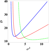
(a)   $d=2$, $\Omega=1$. Continuous, dashed and dot-dashed lines correspond to $\alpha=0,1/2,0.8$, respectively.

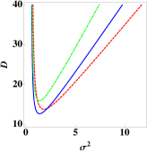
(b)   $\alpha=0$, $\Omega=1$. Continuous, dashed and dot-dashed lines correspond to $d=2,4,6$, respectively.

Figure 1: Phase diagram. Critical lines are defined by $\chi_{0}^{-1}(\sigma^{2},D)=0$, with $\chi_{0}^{-1}$ given by Eq. (16). In the exterior part of each line the system is disordered, $M=0$, while in the interior, $M\neq 0$.

In Figure (1a) we plot the critical line in $d=2$, for different values of the stochastic prescription. Above a minimum lattice coupling $D_{\rm min}$, we found two continuum phase transitions. For very weak noise the system is disordered, $M=0$. At a threshold $\sigma^{2}_{c1}$, the system orders, $M\neq 0$, breaking in this way $Z_{2}$ symmetry. For higher values of the noise, $\sigma^{2}_{c2}>\sigma^{2}_{c1}$ it gets disordered again. Comparing the curve $\alpha=1/2$ with the results of Ref. [32], we conclude that our procedure correctly describes the behavior of $\sigma_{c1}$. In addition, the extension of the ordered region $(\sigma^{2}_{c1}-\sigma^{2}_{c2})$ is much more accurate than usual mean-field approximations. We observe that the ordered area in the $D-\sigma^{2}$ plane growths with $\alpha$. On the other hand, $\sigma^{2}_{c1}$ as well as $\sigma^{2}_{c2}$ are increasing functions of $\alpha$, making the phase transition harder to reach. In fact, in the anti-Itô prescription, $\alpha=1$, $\chi_{0}^{-1}$ is positive definite and there is no phase transition. In Figure (1b), we depict the critical line in the Itô ($\alpha=0$) prescription for different values of the spatial dimension $d$. We observe that $\sigma^{2}_{c1}$ is very weakly dependent on $d$. In fact, for $D\to\infty$, the critical noise rapidly converges to $\sigma^{2}_{c1}=\Omega^{2}/[2(1-\alpha)]$ for any value of $d$. Conversely, $\sigma^{2}_{c2}$ is strongly dependent on dimensionality. Form the integral in Eq. (16), we can see that the dimensionality essentially enter the cut-off as $\Lambda\sim\sqrt{1/d}$. Thus, we can infer the following features on the dependence on the position of the critical line with the cut-off: for greater values of $\Lambda$, the minimum coupling constant $D_{\rm min}$ gets deeper, making easer to reach the phase transition. On the contrary for smaller cut-off, $D_{\rm min}$ rise. In the strongly coupled regime $D>D_{\rm min}$, the threshold for NIPT, $\sigma^{2}_{c1}$, is quite universal, in the sense that is very weakly dependent on the cut-off (in the same way that it is almost independent on $d$, as can be seen from Figure (1b)). However, the “normal” phase transition, $\sigma^{2}_{c2}$, has strongly non-universal behavior.

5 Time reversal and entropy production

It is interesting to characterize the nonequilibrium steady state from the point of view of stochastic thermodynamics [33]. From this perspective, the concept of time reversal stochastic process is essential. For instance, it can be proved that the time reversed evolution of a Markov diffusion process described by an Itô stochastic differential equation is also a Markov diffusion process, however with a different drift [34, 35]. Moreover, we have recently showed [9] that a time reversal transformation of a stochastic process defined by a stochastic differential equation in arbitrary prescription $\alpha$, is perfectly well defined and is given by

$${\cal T}=\left\{\begin{array}[]{lcl}{\bf x}(t)&\to&{\bf x}(-t)\\ &&\\ \alpha&\to&(1-\alpha)\\ &&\\ f_{i}&\to&f_{i}+\left(2\alpha-1\right)\;g_{k\ell}\partial_{k}g_{i\ell}\end{array}\right.$$ (17)

Note that time reversal mixes different prescriptions and, for this reason, it is important to have a formalism that can deal with all prescriptions consistently. With this definition, Crooks relations [23] of microscopic reversibility are satisfied in an equilibrium state reached by a multiplicative Langevin dynamics [8]. Conversely, in a nonequilibrium steady state, such as the one we are studying in this letter, microscopic reversibility is broken and there is an entropy production characterizing this state.

The increase of entropy in the medium, associated with each individual stochastic trajectory [33, 36], can be defined by $\Delta s_{m}=S[{\bf x}]-{\cal T}S[{\bf x}]$, where ${\cal T}S[{\bf x}]$ is the action of the time reversed process [8, 9]. For an equilibrium state, the stochastic entropy is a state function, $\Delta s_{m}=\Delta U=U_{\rm eq}({\bf x}_{f})-U_{\rm eq}({\bf x}_{i})$, where $U_{\rm eq}$ is the equilibrium potential. This is a direct consequence of microscopic reversibility. Explicitly computing $\Delta s_{m}$ for the VPT model, we find

$$\Delta s_{m}=\Delta U[{\bf x}]+\sum_{k}\int_{t_{i}}^{t_{f}}dt\;\dot{x}_{k}\left(\frac{g^{\prime}_{k}}{g_{k}^{3}}\right)W_{\rm os}[{\bf x}]$$ (18)

where $W_{\rm os}({\bf x})=(D/d)\sum_{x_{j}\in n(x_{i})}\left(x_{j}-x_{i}\right)^{2}$ is the potential energy of the lattice coupling and $U(x)=V(x)+W_{\rm os}({\bf x})+(1-\alpha)\ln g^{2}(x)$. Clearly, $\Delta s_{m}$ is not a state function since it depends on the trajectory. The reason behind this behavior is that, in the presence of multiplicative noise, the lattice coupling of the VPT model breaks the Einstein condition, and the stationary state is microscopically irreversible. We argue that microscopic irreversibility and, consequently, the breakdown of detailed-balance, is the main cause of noise-induced phase transitions. To support that, let us analyze two illustrative examples. It is known that in an additive process, $g^{\prime}_{k}=0$, there is no noise-induced phase transition. On the other hand, the last term of Eq. (18) is zero and $\Delta s_{m}$ is a state function. In other words, in the additive noise case, the steady state is an equilibrium one, detailed balance is satisfied, and no NIPT can take place. To stronger support this point of view, let us consider a true multiplicative process with a “slightly” modified lattice coupling,

$$F_{i}({\bf x})=\left(\frac{D}{2d}\right)g^{2}(x_{i})\sum_{x_{j}\in n(x_{i})}\left(x_{j}-x_{i}\right)\;.$$ (19)

This is an harmonic first neighbor interaction locally weighted by the function $g^{2}(x_{i})$. This coupling satisfies Einstein relation since the total drift force can now be written as $f_{k}({\bf x})=-(1/2)g_{k}^{2}\partial_{k}U(\bf x)$. Consequently, the associated entropy is $\Delta s_{m}=U({\bf x}_{f})-U({\bf x}_{i})$, indicating that this system is microscopically reversible. Interestingly, by computing the potential $G_{\rm st}(M)$ and the inverse susceptibility $\chi^{-1}_{0}$, we verify that the latter is positive definite, implying that there is no phase transition in this model.

These facts strongly suggests that microscopic irreversibility of the steady state is a necessary condition for noise-induced phase transitions.

6 Conclusions

We have presented a path integral formalism to compute potentials for nonequilibrium steady states, reached at long times by multiplicative Langevin dynamics. The formalism is completely general and can be applied to study, for any stochastic prescription, a variety of models presenting interesting features, such as noise-induced phase transitions, stochastic resonance and pattern formation. We have also developed a controlled weak noise expansion which correctly captures fluctuation-induced phenomena. In particular, we have analyzed the physics of NIPT by computing the stationary state potential for a general class of lattice models. For the particular VPT model, we have verified that the approximation developed, not only captures the qualitative behavior, but also improves previous estimations for the critical line. Finally, we have shown that microscopic irreversibility is a necessary condition for NIPT phenomena. In such cases, the steady state is characterized by the presence of currents or, equivalently, by a non-zero entropy production rate. This property of the steady state has no relation with the initial stages of the dynamical evolution, in contrast with other interpretations [32], based on the short-time behavior of the order parameter. We believe that the results presented in this letter open many interesting possibilities to advance our understanding of out-of-equilibrium critical phenomena.

- [1] \Namevan Kampen N. G. \BookStochastic Processes in Physics and Chemistry (Elsevier, London, UK) 2007.
- [2] \NameWio H. \BookPath Integrals for Stochastic Processes: An Introduction (World Scientific) 2013.
- [3] \NameKurchan J. \REVIEWJ. Phys. A311998.
- [4] \NameCorberi F., Lippiello E. Zannetti M. \REVIEWJournal of Statistical Mechanics: Theory and Experiment20072007P07002.
- [5] \NameAron C., Barci D. G., Cugliandolo L. F., Gonzalez Arenas Z. Lozano G. S. \REVIEWArXiv e-prints2014arXiv:1412.7564.
- [6] \NameArenas Z. G. Barci D. G. \REVIEWPhys. Rev. E812010051113.
- [7] \NameArenas Z. G. Barci D. G. \REVIEWPhys. Rev. E852012041122.
- [8] \NameArenas Z. G. Barci D. G. \REVIEWJournal of Statistical Mechanics: Theory and Experiment20122012P12005.
- [9] \NameMoreno M. V., Arenas Z. G. Barci D. G. \REVIEWPhys. Rev. E912015042103.
- [10] \NameAron C., Barci D. G., Cugliandolo L. F., Arenas Z. G. Lozano G. S. \REVIEWJournal of Statistical Mechanics: Theory and Experiment20142014P09008.
- [11] \NameJafarpour F., Biancalani T. Goldenfeld N. \REVIEWPhys. Rev. Lett.1152015158101.
- [12] \NameGarcía-Ojalvo J. Sancho J. M. \BookNoise in Spatially Extended Systems (Springer-Verlag, New York) 1999.
- [13] \NameMarro J. Dickman R. \BookNonequilibrium phase transitions in lattice models (Cambridge University Press) 2005.
- [14] \NameDickman R. \REVIEWArXiv e-prints, arXiv/1407.78992014.
- [15] \NameGraham R. \BookMicroscopic potentials, bifurcations, and noise in dissipative systems in \BookNOISE IN NONLINEAR DYNAMICAL SYSTEMS, VOL.1, Ch.7, edited by \NameP.V.E.McClintock F.Moss (Cambridge U. Press, Cambridge, UK.) 1998.
- [16] \NameWio H. S., Deza R. R. Lopez J. M. \BookAn introduction to stochastic processes and nonequilibrium statistical physics; Rev. ed Series on advances in statistical mechanics (World Scientific Publishing, Singapore) 2012.
- [17] \NameWio H., Bouzat S. von Haeften B. \REVIEWPhysica A: Statistical Mechanics and its Applications3062002140 invited Papers from the 21th {IUPAP} International Conference on St atistical Physics.
- [18] \NameWio, H. S. Deza, R. R. \REVIEWEur. Phys. J. Special Topics1462007111.
- [19] \NameLecomte V., Appert-Rolland C. van Wijland F. \REVIEWJournal of Statistical Physics127200751.
- [20] \NameManzano G., Horowitz J. M. Parrondo J. M. R. \REVIEWPhys. Rev. E922015032129.
- [21] \NameVan den Broeck C., Parrondo J. M. R. Toral R. \REVIEWPhys. Rev. Lett.7319943395.
- [22] \NameGenovese W., Muñoz M. A. Sancho J. M. \REVIEWPhys. Rev. E571998R2495.
- [23] \NameCrooks G. E. \REVIEWPhys. Rev. E6120002361.
- [24] \NameLangouche F., Roekaerts D. Tirapegui E. \REVIEWPhysica A: Statistical Mechanics and its Applications951979252.
- [25] \NameF. Langouche D. R. Tirapegui E. \BookFunctional Integration and Semiclassical Expansions (Springer Netherlands) 1982.
- [26] \NameLau A. W. C. Lubensky T. C. \REVIEWPhys. Rev. E762007011123.
- [27] \NameMartin P. C., Siggia E. D. Rose H. A. \REVIEWPhys. Rev. A81973423.
- [28] \NameJanssen H.-K. \REVIEWZeitschrift fÃŒr Physik B Condensed Matter231976377.
- [29] \Namede Dominicis \REVIEWJ. Physique Coll.371976377.
- [30] See appendix A of reference [9] for detailed description of -calculus, such as the generalized chain-rule and integration by parts.
- [31] \NameAppert-Rolland C., Derrida B., Lecomte V. van Wijland F. \REVIEWPhys. Rev. E782008021122.
- [32] \NameVan den Broeck C., Parrondo J. M. R., Toral R. Kawai R. \REVIEWPhys. Rev. E5519974084.
- [33] \NameSeifert U. \REVIEWThe European Physical Journal B - Condensed Matter and Complex Systems642008423.
- [34] \NameU. G. Haussmann E. P. \REVIEWThe Annals of Probability1419861188.
- [35] \NameA. Millet, D. Nualart M. S. \REVIEWThe Annals of Probability171989208.
- [36] \NameVan den Broeck C. Toral R. \REVIEWPhys. Rev. E922015012127.