Mode Gaussian beam tracing

Abstract

An adiabatic mode Helmholtz equation for 3D underwater sound propagation is developed. The Gaussian beam tracing in this case is constructed. The test calculations are carried out for the crosswedge benchmark and proved an excellent agreement with the source images method.

V.I.Il‘ichev Pacific Oceanological Institute, 43, Baltiyskaya Street,

Vladivostok, 690041, Russia

trofimov@poi.dvo.ru, zakharenko@poi.dvo.ru, skozi@poi.dvo.ru

PACS numbers: 43.30.Bp, 43.30.Cq, 43.20.Bi

1 Introduction

The problem of sound propagation across the slope in three dimensions is considered by the method of summation of mode Gaussian beams [1, 2]. In our case, no interaction of modes is necessary to model correctly across slope propagation. The paper is organized as follows. After formulation of the problem in section 2, we consider an adiabatic mode Helmholtz equation and the corresponding parabolic equation in the ray-centered coordinates. In the next section we develop certain details related to the mode Gaussian beams propagation. After that we illustrate the efficiency of the obtained equation by the numerical simulation of sound propagation for the standard ASA wedge benchmark, as it was performed in the paper [3] for the case of the 3D parabolic equation. The paper ends with a brief conclusion.

2 Basic Equations and Boundary Conditions

We consider the propagation of time-harmonic sound in the three-dimensional waveguide

$$\Omega=\{(x,y,z)|0\leq x\leq\infty,-\infty\leq y\leq\infty,-H\leq z\leq 0\}$$

(the $z$-axis is directed upward), described by the acoustic Helmholtz equation

$$\left(\gamma P_{x}\right)_{x}+\left(\gamma P_{y}\right)_{y}+\left(\gamma P_{z}\right)_{z}+\gamma\kappa^{2}P=0\,,$$ (1)

where $\gamma=1/\rho$, $\rho=\rho(x,y,z)$ is the density, $\kappa$ is the wave-number. We assume the appropriate radiation conditions at infinity in the $x,y$ plane, the pressure-release boundary condition $P=0$ at $z=0$ and the rigid boundary condition $\partial P/\partial z=0$ at $z=-H$. The parameters of the medium can be discontinuous at the nonintersecting smooth interfaces $z=h_{1}(x,y),\ldots,h_{m}(x,y)$, where the usual interface conditions

$$\begin{split}&P_{+}=P_{-}\,,\\ &\gamma_{+}\left(\frac{\partial P}{\partial z}-h_{x}\frac{\partial P}{\partial x}-h_{y}\frac{\partial P}{\partial y}\right)_{+}=\gamma_{-}\left(\frac{\partial P}{\partial z}-h_{x}\frac{\partial P}{\partial x}-h_{y}\frac{\partial P}{\partial y}\right)_{-}\,,\end{split}$$ (2)

are imposed. Hereafter, we use the denotations $f(z_{0},x,y)_{+}=\lim_{z\downarrow z_{0}}f(z,x,y)$ and $f(z_{0},x,y)_{-}=\lim_{z\uparrow z_{0}}f(z,x,y)$. As will be seen below, it is sufficient to consider the case $m=1$, so we set $m=1$ and denote $h_{1}$ by $h$.

We introduce a small parameter $\epsilon$ (the ratio of the typical wavelength to the typical size of medium inhomogeneities), the slow variables $X=\epsilon x$ and $Y=\epsilon y$ and the fast variables $\eta=(1/\epsilon)\Theta(X,Y)$ and $\xi=(1/\sqrt{\epsilon})\Psi(X,Y)$ and postulate the following expansions for the acoustic pressure $P$ and the parameters $\kappa^{2}$, $\gamma$ and $h$:

$$\begin{split}&P=P_{0}(X,Y,z,\eta,\xi)+\sqrt{\epsilon}P_{1/2}(X,Y,z,\eta,\xi)+\cdots\,,\\ &\kappa^{2}=n_{0}^{2}(X,Y,z)+\epsilon\nu(X,Y,z,\xi)\,,\\ &\gamma=\gamma_{0}(X,Y,z)+\epsilon\gamma_{1}(X,Y,z,\xi)\,,\\ &h=h_{0}(X,Y)+\epsilon h_{1}(X,Y,\xi)\,.\end{split}$$ (3)

To model attenuation effects, we admit $\nu$ to be complex. Namely, we take $\mathop{\mathrm{Im}}\nu=2\mu\beta n_{0}^{2}\,,$ where $\mu=(40\pi\log_{10}e)^{-1}$ and $\beta$ is the attenuation in decibels per wavelength.

Following the generalized multiple-scale method [4], we replace derivatives in equation (1) by the rules

$$\begin{split}&\frac{\partial}{\partial x}\rightarrow\epsilon\left(\frac{\partial}{\partial X}+\frac{1}{\sqrt{\epsilon}}\Psi_{X}\frac{\partial}{\partial\xi}+\frac{1}{\epsilon}\Theta_{X}\frac{\partial}{\partial\eta}\right)\,,\\ &\frac{\partial}{\partial y}\rightarrow\epsilon\left(\frac{\partial}{\partial Y}\,+\frac{1}{\sqrt{\epsilon}}\Psi_{Y}\frac{\partial}{\partial\xi}+\frac{1}{\epsilon}\Theta_{Y}\frac{\partial}{\partial\eta}\right)\,.\end{split}$$

Given the postulated expansions, the equation under consideration becomes

$$\begin{split}&\epsilon^{2}\left(\frac{\partial}{\partial X}+\frac{1}{\sqrt{\epsilon}}\Psi_{X}\frac{\partial}{\partial\xi}+\frac{1}{\epsilon}\Theta_{X}\frac{\partial}{\partial\eta}\right)\left((\gamma_{0}+\epsilon\gamma_{1})\right.\\ &\quad\cdot\left.\left(\frac{\partial}{\partial X}+\frac{1}{\sqrt{\epsilon}}\Psi_{X}\frac{\partial}{\partial\xi}+\frac{1}{\epsilon}\Theta_{X}\frac{\partial}{\partial\eta}\right)\cdot\left(\vphantom{\frac{\partial}{\partial X}}P_{0}+\epsilon P_{1}+\cdots\,,\right)\right)\\ &+\text{the same term with the $Y$-derivatives}\\ &+\left((\gamma_{0}+\epsilon\gamma_{1})\left(P_{0z}+\epsilon P_{1z}+\cdots\,,\right)\right)_{z}\\ &+(\gamma_{0}+\epsilon\gamma_{1})(n_{0}^{2}+\epsilon\nu)\left(P_{0}+\epsilon P_{1}+\cdots\,,\right)=0\,.\end{split}$$ (4)

We put now

$$\begin{split}P_{0}+\epsilon P_{1}+\cdots=(A_{0}(X,Y,z,\xi)+\epsilon A_{1}(X,Y,z,\xi)+\cdots)\mathrm{e}^{\mathrm{i}\eta}\,.\end{split}$$

Using the Taylor expansion, we can formulate the interface conditions at $h_{0}$ which are equivalent to interface conditions (2) up to $O(\epsilon)$:

$$\left(A_{0}+\epsilon h_{1}A_{0z}+\epsilon A_{1}\right)_{+}=(\text{the same terms})_{-}\,,$$ (5)

$$\begin{split}&\left((\gamma_{0}+\epsilon h_{1}\gamma_{0z}+\epsilon\gamma_{1})\right.\\ &\qquad\qquad\left.\times\left(A_{0z}+\epsilon h_{1}A_{0zz}+\epsilon A_{1z}-\epsilon\mathrm{i}\Theta_{X}h_{0X}A_{0}-\epsilon\mathrm{i}\Theta_{Y}h_{0Y}A_{0}\right)\right)_{+}\\ &=\left(\mbox{the same terms}\right)_{-}\,.\end{split}$$ (6)

2.1 The problem at $O(\epsilon^{0})$

At $O(\epsilon^{0})$ we obtain

$$(\gamma_{0}A_{0z})_{z}+\gamma_{0}n^{2}_{0}A_{0}-\gamma_{0}\left((\Theta_{X})^{2}+(\Theta_{Y})^{2}\right)A_{0}=0\,,$$ (7)

with the interface conditions $A_{0+}=A_{0-}$, $\left(\gamma_{0}A_{0z}\right)_{+}=\left(\gamma_{0}A_{0z}\right)_{-}$ at $z=h_{0}$, and the boundary conditions $A_{0}=0$ at $z=0$ and $A_{0z}=0$ at $z=-H$. We seek a solution to problem (7) in the form

$$A_{0}=B_{j}(X,Y,\xi)\phi(X,Y,z)\,.$$ (8)

From eqs. (7) we obtain the following spectral problem for $\phi$ with the spectral parameter $k^{2}=(\Theta_{X})^{2}+(\Theta_{Y})^{2}$

$$\begin{split}&\left(\gamma_{0}\phi_{z}\right)_{z}+\gamma_{0}n_{0}^{2}\phi-\gamma_{0}k^{2}\phi=0\,,\\ &\phi(0)=0\,,\quad\phi_{z}=0\quad\text{at}\quad z=-H\,,\\ &\phi_{+}=\phi_{-}\,,\quad\left(\gamma_{0}\phi_{z}\right)_{+}=\left(\gamma_{0}\phi_{z}\right)_{-}\quad\mbox{at}\quad z=h_{0}\,.\end{split}$$ (9)

This spectral problem, considering in the Hilbert space $L_{2,\gamma_{0}}[-H,0]$ with the scalar product

$$(\phi,\psi)=\int_{-H}^{\,0}\gamma_{0}\phi\psi\,dz\,,$$ (10)

has countably many solutions $(k_{j}^{2},\phi_{j})$, $j=1,2,\ldots$ where the eigenfunctions can be chosen as real functions. The eigenvalues $k_{j}^{2}$ are real and have $-\infty$ as a single accumulation point. The normalizing condition is

$$(\phi,\phi)=\int_{-H}^{\,0}\gamma_{0}\phi^{2}\,dz=1\,,$$ (11)

2.2 The problem at $O(\epsilon^{1/2})$ and at $O(\epsilon^{1})$

The solvability condition of problem at $O(\epsilon^{1/2})$ is

$$\Theta_{X}\Psi_{X}+\Theta_{Y}\Psi_{Y}=0\,,$$ (12)

from which we conclude that we can take $P_{1/2}=0$.

2.3 The problem at $O(\epsilon^{1})$

At $O(\epsilon^{1})$, we obtain

$$\begin{split}&\left(\gamma_{0}A_{1z}\right)_{z}+\gamma_{0}n_{0}^{2}A_{1}-\gamma_{0}k_{j}^{2}A_{1}\\ &\quad=-\mathrm{i}\gamma_{0X}k_{j}A_{0}-2\mathrm{i}\gamma_{0}k_{j}A_{0X}-\mathrm{i}\gamma_{0}k_{jX}u_{0}+\gamma_{1}k_{j}^{2}A_{0}-\gamma_{0}(\Psi_{X})^{2}A_{0\xi\xi}\\ &\qquad\quad\,-\text{the same terms with $Y$-derivatives}\\ &\qquad\quad\,-\frac{\partial}{\partial z}\left(\gamma_{1}A_{0z}\right)-n_{0}^{2}\gamma_{1}A_{0}-\nu\gamma_{0}A_{0}\,,\end{split}$$ (13)

with the boundary conditions $A_{1}=0$ at $z=0$, $A_{1z}=0$ at $z=-H$, and the interface conditions at $z=h_{0}(X,Y)$:

$$\begin{split}&A_{1+}-A_{1-}=h_{1}(A_{0z-}-A_{0z+})\,,\\ &\gamma_{0+}A_{1z+}-\gamma_{0-}A_{1z-}\\ &\qquad=h_{1}\left(\left((\gamma_{0}A_{0z})_{z}\right)_{-}-\left((\gamma_{0}A_{0z})_{z}\right)_{+}\right)+\gamma_{1-}A_{0z-}-\gamma_{1+}A_{0z+}\\ &\qquad-\mathrm{i}k_{j}h_{0X}A_{0}(\gamma_{0-}-\gamma_{0+})-\mathrm{i}k_{j}h_{0Y}A_{0}(\gamma_{0-}-\gamma_{0+})\,.\end{split}$$ (14)

Multiplying (13) by $\phi_{j}$ and then integrating resulting equation from $-H$ to $0$ by parts twice with the use of interface conditions (14), we obtain the solvability condition for the problem at $O(\epsilon^{1})$

$$\begin{split}&2\mathrm{i}(\Theta_{jX}B_{jX}+\Theta_{jY}B_{jY})+\mathrm{i}(\Theta_{jXX}+\Theta_{jYY})B\\ &\qquad\qquad+((\Psi_{X})^{2}+(\Psi_{Y})^{2})B_{j\xi\xi}+\alpha_{j}B_{j}=0\,,\end{split}$$ (15)

where $A_{0}=B_{j}\phi_{j}$ and $\alpha_{j}$ is given by the following formula

$$\begin{split}&\alpha_{j}=\int_{-\infty}^{0}\gamma_{0}\nu\phi^{2}_{j}\,dz+\int_{-\infty}^{0}\gamma_{1}\left(n_{0}^{2}-k_{j}^{2}\right)\phi^{2}_{j}\,dz-\int_{-\infty}^{0}\gamma_{1}\left(\phi_{jz}\right)^{2}\,dz\\ &+\left\{h_{1}\phi_{j}\left[\left((\gamma_{0}\phi_{jz})_{z}\right)_{+}-\left((\gamma_{0}\phi_{jz})_{z}\right)_{-}\right]\vphantom{\left(\frac{\gamma_{1}}{\gamma_{0}}\right)_{-}}\right.\\ &\qquad\qquad\left.\left.-h_{1}\gamma_{0}^{2}\left(\phi_{jz}\right)^{2}\left[\left(\frac{1}{\gamma_{0}}\right)_{+}-\left(\frac{1}{\gamma_{0}}\right)_{-}\right]\right\}\right|_{z=h_{0}}\,.\end{split}$$

Using spectral problem (9), the interface terms introduced above can be rewritten also as

$$\begin{split}&\left\{h_{1}\phi_{j}^{2}\left[k_{j}^{2}\left(\gamma_{0+}-\gamma_{0-}\right)-\left(n_{0}^{2}\gamma_{0}\right)_{+}+\left(n_{0}^{2}\gamma_{0}\right)_{-}\right]\vphantom{\left(\frac{\gamma_{1}}{\gamma_{0}}\right)_{-}}\right.\\ &\qquad\qquad\left.\left.-h_{1}\gamma_{0}^{2}\left(\phi_{jz}\right)^{2}\left[\left(\frac{1}{\gamma_{0}}\right)_{+}-\left(\frac{1}{\gamma_{0}}\right)_{-}\right]\right\}\right|_{z=h_{0}}\,.\end{split}$$

3 The adiabatic mode Helmholtz equation and the ray parabolic equation in ray centered coordinates

To obtain the adiabatic mode Helmholtz equation from eq. (15), we introduce the new amplitude

$$D_{j}(x,y)=B_{j}(X,Y,\xi)\,,$$

where $\displaystyle{(x,y)=\frac{1}{\epsilon}(X,Y)}$ are the initial (physical) coordinates. One can easily obtain the following formulas for the $x$-derivatives of $D_{j}$:

$$D_{jx}=B_{j\xi}\cdot\sqrt{\epsilon}\Psi_{X}+\epsilon B_{jX}\,,$$ (16)

$$D_{jxx}=B_{j\xi\xi}\cdot\epsilon(\Psi_{X})^{2}+\epsilon^{3/2}(2B_{j\xi X}\Psi_{X}+B_{j\xi}\Psi_{XX})+\epsilon^{2}B_{jXX}\,,$$ (17)

and analogous formulas for the $y$-derivatives.

The solvability condition of the problem at $O(\epsilon^{3/2})$ gives us

$$\begin{split}2B_{j\xi X}\Psi_{X}+B_{j\xi}\Psi_{XX}+2B_{j\xi Y}\Psi_{Y}+B_{j\xi}\Psi_{YY}=0\,.\end{split}$$

Substituting the obtained expressions for derivatives into eq. (15) we get, after some manipulations, the reduced Helmholtz equation for $D$

$$2\mathrm{i}(\theta_{x}D_{jx}+\theta_{x}D_{jy})+\mathrm{i}(\theta_{xx}+\theta_{yy})D_{j}+D_{jxx}+D_{jyy}+\bar{\alpha}_{j}D_{j}=0\,,$$ (18)

where $\theta(x,y)=\frac{1}{\epsilon}\Theta(X,Y)$, $\bar{\alpha}_{j}=\epsilon\alpha_{j}$.

This equation can be transformed to the usual Helmholtz equation

$$\begin{split}\bar{D}_{jxx}+\bar{D}_{jyy}+k^{2}\bar{D}_{j}+\bar{\alpha}_{j}\bar{D}_{j}=0\,,\end{split}$$ (19)

where $k^{2}=(\theta_{x})^{2}+(\theta_{y})^{2}$ by the substitution $\bar{D}_{j}=D_{j}\exp(\mathrm{i}\theta)$. Consider the ray equations for the Hamilton-Jacobi equation

$$(\theta_{x})^{2}+(\theta_{y})^{2}={\cal P}^{2}+{\cal Q}^{2}=k^{2}$$

in the form

$$x_{t}=\frac{{\cal P}}{k}\,,\quad y_{t}=\frac{{\cal Q}}{k}\,,\quad{\cal P}_{t}=k_{x}\,,\quad{\cal Q}_{t}=k_{y}\,.$$ (20)

We have $(x_{t})^{2}+(y_{t})^{2}=1$, so $t$ is a natural parameter for the ray, and introduce $\vec{n}$ to be orthogonal to the ray (ray-centered coordinates).

To obtain the ray parabolic equation in the ray-centered coordinates, we first rewrite eq. (19) in the slow variables $(X,Y)=(\epsilon x,\epsilon y)$ (ray scaling)

$$\begin{split}\epsilon^{2}\bar{D}_{jxx}+\epsilon^{2}\bar{D}_{jyy}+k^{2}\bar{D}_{j}+\epsilon\alpha_{j}\bar{D}_{j}=0\,.\end{split}$$ (21)

Then, in the vicinity of a given ray, eq. (21) can be written in the form

$$\begin{split}\epsilon^{2}\frac{1}{h}(\frac{1}{h}\bar{D}_{jt})_{t}+\epsilon^{2}\frac{1}{h}(h\bar{D}_{jn})_{n}+k^{2}\bar{D}_{j}+\epsilon\alpha_{j}\bar{D}_{j}=0\,,\end{split}$$ (22)

where $t$ is a natural parameter of the ray (arc length), $n$ is the (oriented) distance to the ray and $\displaystyle{h=1-\frac{k_{1}}{k_{0}}}$. Hereafter we use, for a given function $f=f(t,n)$, the following denotations: $f_{0}=f|_{n=0}$, $f_{1}=f_{n}|_{n=0}$ and $f_{2}=f_{nn}|_{n=0}$.

Substituting into eq. (22) the Taylor expansions

$$k^{2}=k_{0}^{2}+2k_{1}k_{0}n+(k_{1}^{2}+k_{0}k_{2})n^{2}=k_{0}^{2}+\sqrt{\epsilon}2k_{1}k_{0}N+\epsilon(k_{1}^{2}+k_{0}k_{2})N^{2}\,,$$

$$\frac{1}{h}=1+\frac{k_{1}}{k_{0}}n+\frac{k_{1}^{2}}{k_{0}^{2}}n^{2}=1+\sqrt{\epsilon}\frac{k_{1}}{k_{0}}N+\epsilon\frac{k_{1}^{2}}{k_{0}^{2}}N^{2}\,,$$

$$\frac{1}{h^{2}}=1+2\frac{k_{1}}{k_{0}}n+3\frac{k_{1}^{2}}{k_{0}^{2}}n^{2}=1+\sqrt{\epsilon}2\frac{k_{1}}{k_{0}}N+\epsilon 3\frac{k_{1}^{2}}{k_{0}^{2}}N^{2}\,,$$

where $\displaystyle{N=\frac{1}{\sqrt{\epsilon}}}$ (parabolic scaling), and the WKB-ansatz $\bar{D}_{j}=(u_{0}+\epsilon u_{1}+\ldots)\exp((\mathrm{i}/\epsilon)\theta)$, we obtain at $O(\epsilon^{0})$

$$\begin{split}\theta_{t}=\mathrm{i}k_{0}\end{split}$$

and at $O(\epsilon^{1})$ the parabolic equation in the ray centered coordinates

$$2\mathrm{i}k_{0}u_{0t}+\mathrm{i}k_{0t}u_{0}+u_{0NN}+[(k_{0}k_{2}-2k_{1}^{2})N^{2}+\alpha_{j0}]u_{0}=0\,.$$ (23)

4 Mode Gaussian Beam Equations

To solve eq. (23), we first introduce the following substitution:

$$u_{0}(t,N)=\frac{1}{\sqrt{k_{0}(t)}}\exp\left(\frac{\mathrm{i}}{2}\int_{0}^{t}\frac{\alpha_{j0}(s)}{k_{0}(s)}\,ds\right)U_{j}(t,N)\,.$$ (24)

Then our equation becomes

$$2\mathrm{i}k_{0}U_{jt}+U_{jNN}+(k_{0}k_{2}-2k_{1}^{2})N^{2}U_{j}=0\,.$$ (25)

Following [1], we seek a solution of this equation in the form of the Gaussian beam anzats

$$U_{j}(t,N)=A(t)\exp\left(\frac{\mathrm{i}}{2}N^{2}\Gamma(t)\right)\,,$$ (26)

where $\Gamma(t)$ is an unknown complex-valued function. Substitution of (26) into (25) gives

$$\mathrm{i}(2k_{0}A_{t}+A\Gamma)-AN^{2}[k_{0}\Gamma_{t}+\Gamma^{2}-(k_{0}k_{2}-2k_{1}^{2})]=0\,.$$

We require separately

$$k_{0}\Gamma_{t}+\Gamma^{2}-(k_{0}k_{2}-2k_{1}^{2})=0\,,\quad\text{and}\quad 2k_{0}A_{t}+A\Gamma=0\,.$$ (27)

To solve the first ordinary non-linear differential equation of the Riccati type, we introduce new complex-valued variables $q(t)$ and $p(t)$ by the formulas

$$\Gamma=\frac{k_{0}}{q}q_{t}=\frac{p}{q}\,.$$

Then

$$q_{t}=k_{0}^{-1}p\,,\qquad p_{t}=(k_{2}-2k_{1}k_{0}^{-1})q\,.$$ (28)

The solution of the second equation in (27) can be expressed in the following form

$$A(t)=\frac{\Psi}{\sqrt{q(t)}}\,,$$

where $\Psi$ is a complex value, which is constant along the ray, but may vary at different rays.

Finally for $u_{0}$ we have:

$$u_{0}(t,N)=\frac{\Psi(\varphi)}{\sqrt{k_{0}(t)q(t)}}\exp\left(\frac{\mathrm{i}}{2}\int_{0}^{t}\frac{\alpha_{j0}(s)}{k_{0}(s)}\,ds+\frac{\mathrm{i}}{2}N^{2}\frac{p(t)}{q(t)}\right)\,.$$ (29)

Here $\varphi$ is the parameter, that enumerates rays. For $p$ and $q$ we have the system of ordinary differential equations (28), which can be solved simultaneously with the ray equations (20). It is convenient to split variables $p$ and $q$ onto real and imaginary parts as follows $p=p_{2}-\mathrm{i}\varepsilon p_{1}$, $q=q_{2}-\mathrm{i}\varepsilon q_{1}$ where $\varepsilon$ is a rather big positive real number, defining the width of the Gaussian beam. As found in [1] and discussed in [2], the optimal choice of $\varepsilon$ for the minimum value of the Gaussian beam width for a homogeneous medium at the point of the receiver corresponds to $\varepsilon=L_{r}$, where $L_{r}$ is the length of the ray to the point of the receiver. Initial conditions for $p$ and $q$ should be following

$$q_{1}(0)=1\,,\quad p_{1}(0)=0\,,\quad q_{2}(0)=0\,,\quad p_{2}(0)=k_{0}(0)\,.$$

The acoustic field at the point of the receiver $M$ can be expressed as the integral on all rays

$$p(M)=\int_{0}^{2\pi}\frac{\Psi(\varphi)}{\sqrt{k_{0}(t)q(t)}}\exp\left[\mathrm{i}\int_{0}^{t}\left(k_{0}(s)+\frac{\alpha_{j0}(s)}{2k_{0}(s)}\right)\,ds+\frac{\mathrm{i}}{2}N^{2}\frac{p(t)}{q(t)}\right]\,d\varphi\,.$$ (30)

Here $t$ and $N$ are the ray centered coordinates of the receiver point for each ray.

One can determine the value of $\Psi(\varphi)$ by comparing of the following two field. First, the one obtained for the homogeneous medium from the formula (30) by the steepest descent method. Second, the one obtained from the fundamental solution of the Helmholtz equation for this case. So we have

$$\Psi=\frac{\phi(z_{s})\phi(z_{r})}{\rho(z_{s})}\cdot\sqrt{\mathrm{i}k_{0}(0)\varepsilon}\cdot\sqrt{1-\frac{\alpha_{j0}(0)x}{2\mathrm{i}k_{0}(0)^{2}\varepsilon}\left(1+\frac{\alpha_{j0}(0)}{2k_{0}(0)^{2}}\right)^{-1}}$$

5 Numerical Example

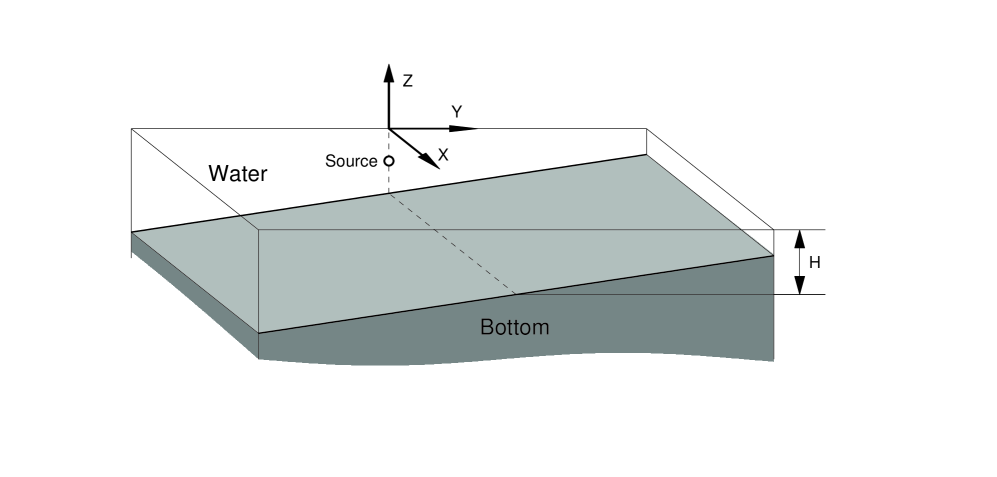
Fig. 1: The geometry for the ASA wedge benchmark. The wedge angle is $\approx 2.86^{\circ}$ with a distance to the apex $4\,km$. The source is located at depth $100\,m.$ The bottom depth at the place of the source $H=200\,m$.

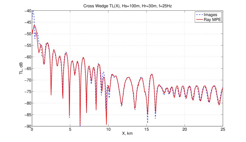
Fig. 2: The transmission loss for the ASA wedge, the source depth is $100\,m.$ The receiver depth is $30\,m$, 3 modes, attenuation is $0.5\,dB/\lambda$. Across slope propagation.

We consider a standard ASA wedge benchmark problem with the angle of wedge $\approx 2.86^{\circ}$ in the case of cross slope propagation (see Fig. 1). The bottom depth is $200\,m$ along the trace with $X=0\ldots 25\,km$. The sound speed in the water is $1500\,m/sec$. The sound speed in the bottom, which is considered liquid, is $1700\,m/sec$. The bottom density is $1500\,kg/m^{3}$, the water density is $1000\,kg/m^{3}$. We assume that there is no attenuation in the water layer, while in the bottom the attenuation is $0.5\,dB/\lambda$. For calculation purposes we restrict the total depth to $600\,m$.

To illustrate the efficiency of our equation, we performed a numerical simulation of sound propagation for the standard ASA wedge benchmark. In fig. 2, we present comparisons of the solution of our equation and the source images solution [5] in the case of cross slope propagation in the wedge with ASA parameters. One can see that the curves are quite close, and the mean square difference between curves is about $1.6\,dB$ in the case of 3 modes. To improve accuracy of the method on the first $1.5\,km$ we can use more than 3 modes. For example, in the case of 7 modes, the field in the vicinity of the source is represented correctly, and the mean square difference is about $1.4\,dB$.

6 Conclusions

The results of test calculations show, that the acoustic field in the far zone is satisfactory described by its first three modes. We have shown that no interaction of modes is necessary to perform satisfactory modeling of a cross slope propagation. However, to obtain a more realistic model, we assert, that seven modes (total depth is $600\,m$) are sufficient to represent the acoustic field in the all considered area.

References

• [1] V. Červený, M. M. Popov, I. Pšenčík, Computation of wave fields in inhomogeneous media - gauss beam approach // Geophys. J. R. astr. Soc. 70 (1982) 109–128.
• [2] M. B. Porter, H. P. Bucker, Gaussian beam tracing for computing ocean acoustic fields // J. Acoust. Soc. Am. 82 (4) (1987) 1349–1359.
• [3] Y. T. Lin, J. M. Collis, T. F. Duda, A three-dimensional parabolic equation model of sound propagation using higher-order operator splitting and padé approximants // J. Acoust. Soc. Am. 132 (5) (2012) EL364–EL370.
• [4] A. H. Nayfeh, Perturbation methods, John Wiley and Sons, New York, London, Sydney, Toronto, 1973.
• [5] G. B. Deane, M. J. Buckingham, An analysis of the three dimensional sound field in a penetrable wedge with a stratified fluid or elastic basement // J. Acoust. Soc. Am. 93 (1993) 1319–1328.