Self-energy effects in functional renormalization group flows of the two-dimensional $t$-$t^{\prime}$ Hubbard model away from van Hove filling

Abstract

We study the impact of the fermionic self-energy on one-loop functional renormalization group flows of the two-dimensional $t$-$t^{\prime}$ Hubbard model, with emphasis on electronic densities away from van Hove filling. In the presence of antiferromagnetic hot spots, antiferromagnetic fluctuations lead to a flattening of the Fermi surface, shift magnetic phase boundaries and significantly enhance critical scales. We trace back this effect to the presence of a magnetic first order transition. For some parameters, the first order character of the latter is reduced by self-energy effects. For reliably determining phase diagrams, the fermionic self-energy should be taken into account in functional renormalization group studies if scattering between hot spots is important.

I Introduction

The Hubbard model is a paradigmatic model system for the description of correlated electrons in solids. Despite the simplicity of the model, an exact solution is only available in one spatial dimension. The two-dimensional model is believed to contain the essential ingredients to describe high-temperature superconductivity in cuprates. Similar to these materials, the model shows antiferromagnetism in its ground state at half-filling and becomes superconducting when sufficiently doped away from half-filling Scalapino (2012). The lightly doped regime of cuprate materials and the Hubbard model are, however, relatively poorly understood. Achieving an accurate description of the properties of the Hubbard model in this regime is therefore highly desirable.

Recent progress in the development of some numerical methods allowed to achieve agreement between the results in certain parameter regimes, but discrepancies remain for the important intermediate coupling regime at small doping LeBlanc et al. (2015). In this regime, several different states have very similar energies and an accurate determination of the ground state is difficult. One source of difficulty is the limitation of many numerical methods to relatively small systems. It therefore seems useful to complement numerical studies of the model with more analytical approaches that have access to low-energy Fermi surface instabilities in the thermodynamic limit. One such method is the functional renormalization group Wetterich (1993); Salmhofer and Honerkamp (2001); Metzner et al. (2012) (fRG).

This method treats all interaction channels on equal footing and is thus well suited for the study of competing order. One of its major successes was the unbiased detection of $d$-wave superconductivity in the ground state of the two-dimensional Hubbard model at weak coupling Metzner et al. (2012); Friederich et al. (2011); Eberlein and Metzner (2014). Results at weak coupling cannot be directly transferred to the cuprates, but allow to understand some qualitative features of their phase diagram in a controlled way. Until recently, the applicability of available truncation schemes of the fRG flow equations was limited to weak coupling, but this restriction may be removed by using non-trivial starting points for the fRG flow Machado and Dupuis (2010); Taranto et al. (2014); Wentzell et al. (2015).

Most fRG studies for itinerant fermionic systems used a one-loop truncation, in which the fermionic self-energy and the two-particle vertex are renormalized Katanin (2004); Metzner et al. (2012). Motivated by the fact that the information on most continuous phase transitions is encoded in the momentum dependence of the vertex, which diverges with the correlation length for certain combinations of momenta, the self-energy was usually neglected. A few studies investigated the influence of the self-energy on the flow and focused on the parameter region around van Hove filling. A general tendency towards a flattening of the Fermi surface was found in an early study slightly above van Hove filling, which however neglected the feedback of the self-energy on the flow Honerkamp et al. (2001). More recent studies included the self-energy feedback on the flow, but were mostly restricted to a small region around van Hove filling, where interesting effects like competing instabilities or non-Fermi liquid behavior may already occur at weak coupling Igoshev et al. (2011); Husemann et al. (2012); Giering and Salmhofer (2012). In this parameter regime, it was found that renormalizing the Fermi surface has only a very small impact on the flow.

Despite the fact that deformations of the Fermi surface are important perturbations in two-dimensional systems, their impact on functional renormalization group flows away from van Hove filling has not been fully addressed, yet. Knowing the impact of the self-energy on fRG flows in a broader parameter regime is certainly useful to judge the reliability of flows with perturbative as well as non-trivial starting points. Moreover, the one-loop fRG was also applied to model systems for the description of unconventional superconductivity in pnictide and ruthenate materials Platt et al. (2013) and used to provide an explanation for subtle features in the momentum dependence of the superconducting gap. As these works neglected the fermionic self-energy, it would be interesting to know how robust their results are if the self-energy were taken into account.

In this work, we study the impact of the self-energy on one-loop fRG flows away from van Hove filling and at zero temperature. As in former studies, flows at van Hove filling are not changed qualitatively when the Fermi surface is renormalized. A similar conclusion holds for electron fillings below van Hove filling. In the presence of antiferromagnetic hot spots, i. e. intersection points of the Fermi surface and the boundary of the magnetic Brillouin zone, the renormalization of the Fermi surface via the self-energy has a sizable quantitative impact on critical scales and shifts the boundaries between regimes with different leading instabilities. This is caused by a flattening of the Fermi surface, which leads to improved nesting and enhances antiferromagnetic fluctuations, thereby enlarging the parameter regime with antiferromagnetism as leading instability. Combining fRG flows with a mean-field (MF) analysis Reiss et al. (2007); Wang et al. (2014) for the magnetic phase diagram, we trace back the large impact of the self-energy on the flow to the presence of a magnetic first-order phase transition.

This paper is organized as follows. Section II briefly introduces the Hubbard model and the fRG. Section III describes results mostly from one-loop flows in static approximation, i. e. where the frequency dependence of the vertex and the self-energy are neglected, as well as results from a combination of fRG and mean-field theory. A few results from a dynamic approximation are also discussed. Section IV contains a summary and conclusions.

II Model and Method

II.1 Model

The Hubbard model describes spin-$\tfrac{1}{2}$ fermions with a local repulsive interaction on a lattice. Its Hamiltonian in second-quantization notation is given by

$$H=\sum_{i,j,\sigma}t_{ij}c^{\dagger}_{i\sigma}c_{j\sigma}+U\sum_{i}n_{i\uparrow}n_{i\downarrow},$$ (1)

where $c^{(\dagger)}_{i\sigma}$ are annihilation (creation) operators for fermions with spin orientation $\sigma=\uparrow,\downarrow$ on lattice site $i$. We study this model on a two-dimensional square lattice and restrict the hopping of fermions $t_{ij}$ to nearest and next-nearest neighbor sites with amplitudes $-t$ and $-t^{\prime}$, respectively. Fourier transformation of the hopping matrix yields the dispersion

$$\epsilon(\boldsymbol{k})=-2t(\cos k_{x}+\cos k_{y})-4t^{\prime}\cos k_{x}\cos k_{y}.$$ (2)

Fermions occupying the same lattice site interact via the local Coulomb interaction with strength $U$.

In the following, we set $t\equiv 1$ and use it as the unit of energy.

II.2 Functional renormalization group

The functional renormalization group allows to resum perturbation theory in a scale-separated way and treats all interaction channels on an equal footing. Comprehensive introductions to the method can be found in Refs. Berges et al., 2002; Metzner et al., 2012; Platt et al., 2013; Kopietz et al., 2010.

The starting point of the method is a functional flow equation for the effective action Wetterich (1993); Salmhofer and Honerkamp (2001), the generating functional of one-particle irreducible (1PI) vertex functions. The functional flow equation is equivalent to an infinite hierarchy of flow equations for vertex functions. Truncating this hierarchy and formulating an ansatz for the effective action allows to derive a closed set of renormalization group equations for the latter.

In this work, we employ a truncation at the two-particle level, in which self-energy feedback from the three-particle level is taken into account Katanin (2004). Assuming translational and spin rotation invariance, we formulate the ansatz

$$\begin{split}&\Gamma^{\Lambda}[\bar{\psi},\psi]=\Gamma^{(0)\,\Lambda}+\sum_{k,\sigma}\Gamma^{(2)\,\Lambda}(k)\bar{\psi}_{k\sigma}\psi_{k\sigma}\\ &+\frac{1}{4}\sum_{k_{i},\sigma_{i}}\Gamma^{(4)\,\Lambda}_{\sigma_{1}\sigma_{2}\sigma_{3}\sigma_{4}}(k_{1},k_{2},k_{3},k_{4})\bar{\psi}_{k_{1}\sigma_{1}}\bar{\psi}_{k_{2}\sigma_{2}}\psi_{k_{3}\sigma_{3}}\psi_{k_{4}\sigma_{4}}\end{split}$$ (3)

for the effective action, where $k=(k_{0},\boldsymbol{k})$ combines Matsubara frequencies and momenta. Due to symmetries, the two-particle vertex $\Gamma^{(4)\,\Lambda}$ is non-zero only for $k_{1}+k_{2}=k_{3}+k_{4}$ and $\sigma_{1}=\sigma_{4}$, $\sigma_{2}=\sigma_{3}$ or $\sigma_{1}=\sigma_{3}$, $\sigma_{2}=\sigma_{4}$.

The regularized fermionic propagator $G^{\Lambda}(k)=-(\Gamma^{(2)\,\Lambda})^{-1}(k)$ is related to the regularized bare propagator $G_{0}^{\Lambda}(k)$ and the self-energy $\Sigma^{\Lambda}(k)$ via a Dyson equation,

$$(G^{\Lambda})^{-1}(k)=(G_{0}^{\Lambda})^{-1}(k)-\Sigma^{\Lambda}(k).$$ (4)

The regularized bare propagator is given by

$$(G^{\Lambda}_{0})^{-1}(k)=ik_{0}-\epsilon(\boldsymbol{k})+\mu+R^{\Lambda}(k),$$ (5)

where $\mu$ is the chemical potential and $R^{\Lambda}$ the regulator. We use an additive frequency regulator,

$$R^{\Lambda}(k)=i\operatorname{sgn}(k_{0})\sqrt{k_{0}^{2}+\Lambda^{2}}-ik_{0},$$ (6)

that replaces small frequencies $k_{0}$ by $\operatorname{sgn}(k_{0})\Lambda$ in $(G^{\Lambda}_{0})^{-1}$. This regulator has been used in several works before Eberlein and Metzner (2013, 2014); Eberlein (2014); Maier et al. (2014) and it was found that critical scales for pairing instabilities provide a very good estimate for the maximum amplitude of the ground state pairing gap.

Within the truncation scheme proposed by Katanin Katanin (2004), we obtain flow equations for the self-energy,

$$\frac{d}{d\Lambda}\Sigma^{\Lambda}(k)=\sum_{\sigma}\int\negthickspace\negthinspace\frac{d^{3}p}{(2\pi)^{3}}\Gamma^{(4)\,\Lambda}_{\uparrow\sigma\sigma\uparrow}(k,p,p,k)S^{\Lambda}(p),$$ (7)

where $S^{\Lambda}(k)=\frac{d}{d\Lambda}G^{\Lambda}(k)|_{\Sigma^{\Lambda}=\operatorname{const.}}$ is the fermionic single-scale propagator, and the two-particle vertex

$$\frac{d}{d\Lambda}\Gamma^{(4)\,\Lambda}_{\sigma_{1}\sigma_{2}\sigma_{3}\sigma_{4}}(k_{1},k_{2},k_{3},k_{4})=\Pi^{\text{PH},d}_{\sigma_{1}\sigma_{2}\sigma_{3}\sigma_{4}}(k_{1},k_{2},k_{3},k_{4})-\Pi^{\text{PH},cr}_{\sigma_{1}\sigma_{2}\sigma_{3}\sigma_{4}}(k_{1},k_{2},k_{3},k_{4})-\frac{1}{2}\Pi^{\text{PP}}_{\sigma_{1}\sigma_{2}\sigma_{3}\sigma_{4}}(k_{1},k_{2},k_{3},k_{4}),$$ (8)

where the contributions on the right hand side are the direct particle-hole, crossed particle-hole and particle-particle diagram, respectively. They are given by

$$\begin{split}\Pi^{\text{PH},d}_{\sigma_{1}\sigma_{2}\sigma_{3}\sigma_{4}}(k_{1},k_{2},k_{3},k_{4})&=\sum_{p,\sigma_{1}^{\prime},\sigma_{2}^{\prime}}\frac{d}{d\Lambda}\Bigl{(}G^{\Lambda}(p-\tfrac{q}{2})G^{\Lambda}(p+\tfrac{q}{2})\Bigr{)}\Gamma^{(4)\,\Lambda}_{\sigma_{1}\sigma_{1}^{\prime}\sigma_{2}^{\prime}\sigma_{4}}\bigl{(}k_{1},p-\tfrac{q}{2},p+\tfrac{q}{2},k_{4}\bigr{)}\\ &\hskip 50.00008pt\times\Gamma^{(4)\,\Lambda}_{\sigma_{2}^{\prime}\sigma_{2}\sigma_{3}\sigma_{1}^{\prime}}\bigl{(}p+\tfrac{q}{2},k_{2},k_{3},p-\tfrac{q}{2}\bigr{)}|_{q=k_{3}-k_{2}}\\ &=\Pi^{\text{PH},cr}_{\sigma_{2}\sigma_{1}\sigma_{3}\sigma_{4}}(k_{2},k_{1},k_{3},k_{4})\end{split}$$ (9)

$$\begin{split}\Pi^{\text{PP}}_{\sigma_{1}\sigma_{2}\sigma_{3}\sigma_{4}}(k_{1},k_{2},k_{3},k_{4})&=\sum_{p,\sigma_{1}^{\prime},\sigma_{2}^{\prime}}\frac{d}{d\Lambda}\Bigl{(}G^{\Lambda}(\tfrac{q}{2}-p)G^{\Lambda}(\tfrac{q}{2}+p)\Bigr{)}\Gamma^{(4)\,\Lambda}_{\sigma_{1}\sigma_{2}\sigma_{2}^{\prime}\sigma_{1}^{\prime}}(k_{1},k_{2},\tfrac{q}{2}-p,\tfrac{q}{2}+p)\\ &\hskip 50.00008pt\times\Gamma^{(4)\,\Lambda}_{\sigma_{1}^{\prime}\sigma_{2}^{\prime}\sigma_{3}\sigma_{4}}(\tfrac{q}{2}+p,\tfrac{q}{2}-p,k_{3},k_{4})|_{q=k_{1}+k_{2}}.\end{split}$$ (10)

Within this truncation, on the right hand side of the flow equation the scale-derivative of the full propagator,

$$\frac{d}{d\Lambda}G^{\Lambda}(k)=S^{\Lambda}(k)+G^{\Lambda}(k)\dot{\Sigma}^{\Lambda}(k)G^{\Lambda}(k),$$ (11)

appears instead of the single-scale propagator. This leads to a better treatment of self-energy corrections Katanin (2004).

In order to make the flow equations amenable for a numerical solution, we decompose the vertex into interactions channels and derive flow equations for the effective interaction in each channel as described in Refs. Karrasch et al., 2008; Husemann and Salmhofer, 2009. Our ansatz and notation are very similar to those of Ref. Eberlein and Metzner, 2014. We write

$$\begin{split}\Gamma^{(4)\,\Lambda}_{\sigma_{1}\sigma_{2}\sigma_{3}\sigma_{4}}&(k_{1},k_{2},k_{3},k_{4})=u_{\sigma_{1}\sigma_{2}\sigma_{3}\sigma_{4}}(k_{1},k_{2},k_{3},k_{4})\\ &+V^{\text{PH},\Lambda}_{\sigma_{1}\sigma_{2}\sigma_{3}\sigma_{4}}(\tfrac{k_{1}+k_{4}}{2},\tfrac{k_{2}+k_{3}}{2};k_{3}-k_{2})\\ &-V^{\text{PH},\Lambda}_{\sigma_{2}\sigma_{1}\sigma_{3}\sigma_{4}}(\tfrac{k_{2}+k_{4}}{2},\tfrac{k_{1}+k_{3}}{2};k_{3}-k_{1})\\ &+V^{\text{PP},\Lambda}_{\sigma_{1}\sigma_{2}\sigma_{3}\sigma_{4}}(\tfrac{k_{1}-k_{2}}{2},\tfrac{k_{4}-k_{3}}{2};k_{1}+k_{2}).\end{split}$$ (12)

for the vertex, where $u$ is the antisymmetrized bare interaction, and $V^{\text{PH},\Lambda}$ and $V^{\text{PP},\Lambda}$ describe fluctuation corrections in the particle-hole and particle-particle channels, respectively. The first two momentum arguments of the latter two functions are fermionic relative momenta while the third is a bosonic momentum transfer or total momentum. For the Hubbard model, $u$ reads

$$\begin{split}u_{\sigma_{1}\sigma_{2}\sigma_{3}\sigma_{4}}(k_{1},k_{2},k_{3},k_{4})&=U\delta_{k_{1}+k_{2},k_{3}+k_{4}}\\ &\times(\delta_{\sigma_{1}\sigma_{4}}\delta_{\sigma_{2}\sigma_{3}}-\delta_{\sigma_{1}\sigma_{3}}\delta_{\sigma_{2}\sigma_{4}}).\end{split}$$ (13)

For the fluctuation corrections in the particle-hole channel, we make the ansatz

$$\begin{split}V^{\text{PH},\Lambda}_{\sigma_{1}\sigma_{2}\sigma_{3}\sigma_{4}}(k,k^{\prime};q)&=(2\delta_{\sigma_{1}\sigma_{3}}\delta_{\sigma_{2}\sigma_{4}}-\delta_{\sigma_{1}\sigma_{4}}\delta_{\sigma_{2}\sigma_{3}})M^{\Lambda}_{kk^{\prime}}(q)\\ &\ +\delta_{\sigma_{1}\sigma_{4}}\delta_{\sigma_{2}\sigma_{3}}C^{\Lambda}_{kk^{\prime}}(q),\end{split}$$ (14)

where $C^{\Lambda}$ and $M^{\Lambda}$ are a density-density interaction $\sim nn$ and a spin-spin interaction $\sim\boldsymbol{s}\cdot\boldsymbol{s}$, respectively. The ansatz for the fluctuation corrections in the particle-particle channel reads

$$\begin{split}V^{\text{PP},\Lambda}_{\sigma_{1}\sigma_{2}\sigma_{3}\sigma_{4}}(k,k^{\prime};q)&=\delta_{\sigma_{1}\sigma_{4}}\delta_{\sigma_{2}\sigma_{3}}P^{\Lambda}_{kk^{\prime}}(q)\\ &-\delta_{\sigma_{1}\sigma_{3}}\delta_{\sigma_{2}\sigma_{4}}P^{\Lambda}_{k,-k^{\prime}}(q).\end{split}$$ (15)

Inserting these ansatzes into the flow equation for the vertex and assigning diagrams to interaction channels according to the transfer momenta in the fermionic loop integrals, we obtain the flow equations

$$\frac{d}{d\Lambda}P^{\Lambda}_{kk^{\prime}}(q)=-\frac{1}{2}\Pi^{\text{PP},\Lambda}_{\uparrow\downarrow\downarrow\uparrow}(k+\tfrac{q}{2},\tfrac{q}{2}-k,\tfrac{q}{2}-k^{\prime},k^{\prime}+\tfrac{q}{2}),$$ (16)

$$\frac{d}{d\Lambda}M^{\Lambda}_{kk^{\prime}}(q)=\frac{1}{2}\Pi^{\text{PH},d}_{\uparrow\downarrow\uparrow\downarrow}(k+\tfrac{q}{2},k^{\prime}-\tfrac{q}{2},k^{\prime}+\tfrac{q}{2},k-\tfrac{q}{2}),$$ (17)

$$\begin{split}\frac{d}{d\Lambda}C^{\Lambda}_{kk^{\prime}}(q)&=\Pi^{\text{PH},d}_{\uparrow\downarrow\downarrow\uparrow}(k+\tfrac{q}{2},k^{\prime}-\tfrac{q}{2},k^{\prime}+\tfrac{q}{2},k-\tfrac{q}{2})\\ &+\frac{d}{d\Lambda}M^{\Lambda}_{kk^{\prime}}(q).\end{split}$$ (18)

More detailed expressions for the flow equations can be found in Appendix A.

II.3 Approximation scheme for vertex and self-energy

In the following we describe the approximations and parametrizations for the vertex and the self-energy that are applied within the channel-decomposition scheme. The framework of approximations is very similar to that in Refs. Eberlein and Metzner, 2013, 2014. Differently from these works, we do not introduce order parameters and analyze the leading instabilities of the flow.

The fluctuation corrections in the particle-hole and particle-particle channels are described as boson-mediated interactions. Former fRG studies identified the $s$- and $d_{x^{2}-y^{2}}$-wave channels as those yielding the largest contributions to the flow in the parameter regime that is relevant in this work Zanchi and Schulz (2000); Halboth and Metzner (2000a); Honerkamp et al. (2001); Husemann and Salmhofer (2009); Giering and Salmhofer (2012). For the pairing, magnetic and charge fluctuations, we make the ansatzes

$$P^{\Lambda}_{kk^{\prime}}(q)=P^{\Lambda}_{s}(q)+P^{\Lambda}_{d}(q)f_{d}(\boldsymbol{k})f_{d}(\boldsymbol{k}^{\prime}),$$ (19)

$$M^{\Lambda}_{kk^{\prime}}(q)=M^{\Lambda}_{s}(q)+M^{\Lambda}_{d}(q)f_{d}(\boldsymbol{k})f_{d}(\boldsymbol{k}^{\prime}),$$ (20)

$$C^{\Lambda}_{kk^{\prime}}(q)=C^{\Lambda}_{s}(q)+C^{\Lambda}_{d}(q)f_{d}(\boldsymbol{k})f_{d}(\boldsymbol{k}^{\prime}),$$ (21)

where $f_{d}(\boldsymbol{k})=\cos k_{x}-\cos k_{y}$ is a lattice form factor with $d$-wave symmetry. The exchange propagators $P^{\Lambda}_{i}$, $M^{\Lambda}_{i}$ and $C^{\Lambda}_{i}$ describe mediated interactions in the $s$- and $d$-wave channels. The second contribution in the charge channel captures density-wave fluctuations with a $d$-wave form factor Halboth and Metzner (2000a); Husemann and Metzner (2012); Sachdev and La Placa (2013); Meier et al. (2014).

In this work we discuss two approximation schemes: A dynamic and a static approximation. In the dynamic approximation, we keep the dependence of the exchange propagators on the bosonic frequency $q_{0}$ and also the frequency dependence of the self-energy. In the static approximation, we neglect all frequency dependences and evaluate the exchange propagators at $q_{0}=0$. More details on the description of the momentum and frequency dependence of exchange propagators and the numerical solution of the flow equations can be found in Appendix B.

The central theme of this paper is to study the impact of the fermionic self-energy on fRG flows away from van Hove filling. We thus like to keep track of interaction-induced deformations of the Fermi surface, but also of the renormalization of the fermionic quasiparticles. At low scales we expect the momentum dependence of the self-energy parallel to the Fermi surface to be more important than the dependence perpendicular to it, and thus neglect the latter. We subdivide the Brillouin zone into patches (as in the $N$-patch approximation for the vertex Zanchi and Schulz (2000)) and evaluate the self-energy $\Sigma^{\Lambda}(k)$ in each patch for the Fermi momentum in the middle of the patch. The frequency dependence is discretized on a non-equidistant grid with higher density of grid points at low frequencies, as for the exchange propagators. This reduces the self-energy in the dynamic approximation to a two-dimensional function of frequency and angle along the Fermi surface. At intermediate points, the self-energy is determined by linear interpolation. In the static approximation, the one-loop flow does not generate a frequency dependence of the self-energy and we evaluate it at $k_{0}=0$. The same approximations as for $\Sigma^{\Lambda}(k)$ are used for $\frac{d}{d\Lambda}\Sigma^{\Lambda}(k)$ appearing in the scale-differentiated propagator on the right hand side of the flow equations. In Sec. III, we compare results from fRG flows using these approximations for the self-energy with results from fRG flows using different approximations like neglecting the self-energy completely. The latter approximation is widely used in the literature.

III Results

In this section, we present results from a numerical solution of the flow equations for the ground state. We discuss the dependence of critical scales $\Lambda_{c}$ on the next-nearest neighbor hopping $t^{\prime}$, the fermionic density $n$ and various approximations for the self-energy $\Sigma$. We present results for a moderate interaction strength $U=3$. The critical scale $\Lambda_{c}$ is defined as the scale $\Lambda$ where the largest component of exchange propagators exceeds $50t$. When extrapolating the flow, it would diverge at slightly lower scales. All flows were evaluated in the presence of a fixed chemical potential $\mu$ and the fermionic density was determined from the full fermionic propagator at the critical scale.

In the following, we first discuss results for critical scales from static one-loop flows. In order to reduce the impact of the choice of the regulator on our conclusions, we compare the established trends with mean-field calculations that take the fRG results as input. At the end of this section we briefly discuss results from a dynamic one-loop approximation where the vertex and the self-energy also depend on frequency.

III.1 Static one-loop flows

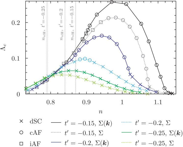
Figure 1: (Color online) Critical scales $\Lambda_{c}$ of one-loop fRG flows in static approximation for $U=3$ and different values of $t^{\prime}$. For each value of $t^{\prime}$, critical scales from flows with momentum-dependent self-energy $\Sigma^{\Lambda}(\boldsymbol{k})$ (labeled “$\Sigma(\boldsymbol{k})$”, full lines) and with momentum-independent self-energy $\Sigma^{\Lambda}(\boldsymbol{k})=\Sigma^{\Lambda}$ (labeled “$\Sigma$”, dashed lines) are compared. Symbols represent the leading instability (crosses for d-wave superconductivity (dSC), circles for commensurate antiferromagnetism (cAF) and squares for incommensurate antiferromagnetism(iAF)). The vertical dashed lines mark van Hove filling for the different values of $t^{\prime}$.

In the following, we present results from static one-loop flows. In Fig. 1 we compare critical scales $\Lambda_{c}$ as obtained from flows with momentum-dependent ($\Sigma^{\Lambda}(\boldsymbol{k})$) or momentum-independent ($\Sigma^{\Lambda}(\boldsymbol{k})=\Sigma^{\Lambda}$ computed as Fermi surface average) self-energy for $U=3$ and different values of $t^{\prime}$. As discussed below (see Fig. 6), the latter results are very close to those obtained from flows where the self-energy is neglected completely. The filling where the saddle points of the fermionic dispersion are part of the Fermi surface (van Hove filling) plays an important role in deciding how large the impact of a momentum-dependent renormalization of the self-energy is. We define van Hove filling as the filling where the saddle points are part of the renormalized Fermi surface at the critical scale, as in Ref. Giering and Salmhofer, 2012. This is the case for $n_{\text{vH}}=0.87$ for $t^{\prime}=-0.15$, $n_{\text{vH}}=0.83$ for $t^{\prime}=-0.2$ and $n_{\text{vH}}=0.79$ for $t^{\prime}=-0.25$. For electron densities near van Hove filling, the renormalization of the self-energy practically does not influence the critical scale, in agreement with the literature Giering and Salmhofer (2012). This is different closer to half-filling, where antiferromagnetic hot spots exist. When taking the momentum dependence of the self-energy into account, the parameter region with a leading instability towards antiferromagnetism is enlarged and the critical scale significantly enhanced for the smaller values of $-t^{\prime}$. For $t^{\prime}=-0.25$, no magnetic instability is found in both approximations, but antiferromagnetic fluctuations and the critical scale for $d$-wave pairing are also enhanced.

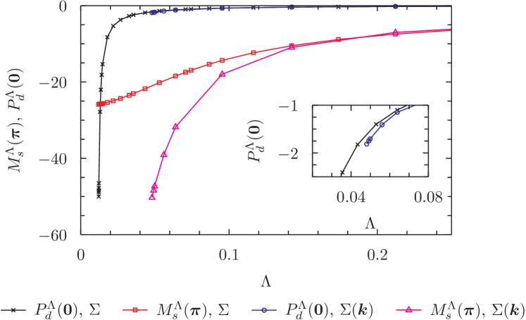
Figure 2: (Color online) Flow of exchange propagators in the magnetic channel $M^{\Lambda}_{s}(\boldsymbol{q}=\boldsymbol{\pi})$ and in the $d$-wave pairing channel $P^{\Lambda}_{d}(\boldsymbol{q}=\boldsymbol{0})$ for $U=3$, $t^{\prime}=-0.15$ and $n=1.1$ as computed with renormalization of the momentum dependence of the self-energy $\Sigma^{\Lambda}(\boldsymbol{k})$ (labeled “$\Sigma(\boldsymbol{k})$”) and by approximating the self-energy as momentum independent (labeled “$\Sigma$”). The pairing interaction close to the critical scale of the flow with momentum-dependent self-energy is shown in the inset.

On the electron-doped side, the leading instability can change from $d$-wave superconductivity to antiferromagnetism when renormalizing the Fermi surface. An exemplary flow of some couplings for such a case is shown in Fig. 2. Using the momentum-independent approximation for the self-energy, the effective interaction in the magnetic channel saturates towards low scales and the $d$-wave pairing interaction eventually grows very strongly. Taking the momentum dependence of $\Sigma^{\Lambda}$ into account leads to a strong enhancement of antiferromagnetic fluctuations and eventually to a magnetic instability. At the critical scale of the latter flow, the $d$-wave pairing interaction is also enhanced by roughly $20\%$. For these parameters, the Fermi surface at the hot spots is not perfectly nested and the particle-hole bubble with transfer momentum $\boldsymbol{q}=\boldsymbol{\pi}$ thus finite, so that driving an antiferromagnetic instability requires a minimal coupling strength. In the flow with momentum-independent self-energy, the bare $U$ is effectively reduced by fluctuations below this threshold. In the momentum-dependent case, the renormalization of the Fermi surface leads to improved nesting around the hot spots, which in turn enhances antiferromagnetic fluctuations and gives rise to a magnetic instability.

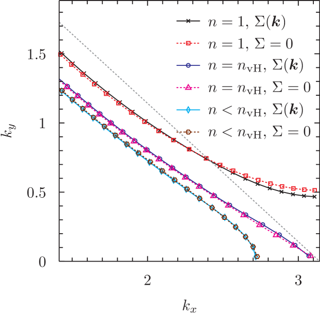
Figure 3: (Color online) Renormalized and bare Fermi surfaces from static one-loop fRG flows at the critical scale $\Lambda_{c}$ for $U=3$ and $t^{\prime}=-0.2$ for different electron fillings below van Hove filling ($n=0.76$, $\Lambda_{c}=0.02$), at van Hove filling ($n=n_{\text{vH}}=0.83$, $\Lambda_{c}=0.079$) and at half-filling ($n=1$, $\Lambda_{c}=0.103$). Renormalized (bare) Fermi surfaces are shown with full (dashed) lines and are labeled “$\Sigma(\boldsymbol{k})$” (“$\Sigma=0$”).

The improvement of nesting is mainly caused by antiferromagnetic fluctuations and can be seen in Fig. 3. In this figure, we compare the bare and renormalized Fermi surfaces for $U=3$, $t^{\prime}=-0.2$ and different fermionic densities. The deformation of the Fermi surface for the parameters used in Fig. 2 is qualitatively very similar to that for $n=1$ in Fig. 3. At half-filling and van Hove filling ($n=n_{\text{vH}}$), the Fermi surface is flattened around the hot spots or the saddle points. A flattening of the Fermi surface around hot spots due to strong antiferromagnetic fluctuations was also observed before in the Hubbard model Neumayr and Metzner (2003); Honerkamp et al. (2001) and close to a spin-density wave quantum critical point with ordering wave vector $(\pi,\pi)$ in the spin-fermion model Abanov and Chubukov (2000); Metlitski and Sachdev (2010).

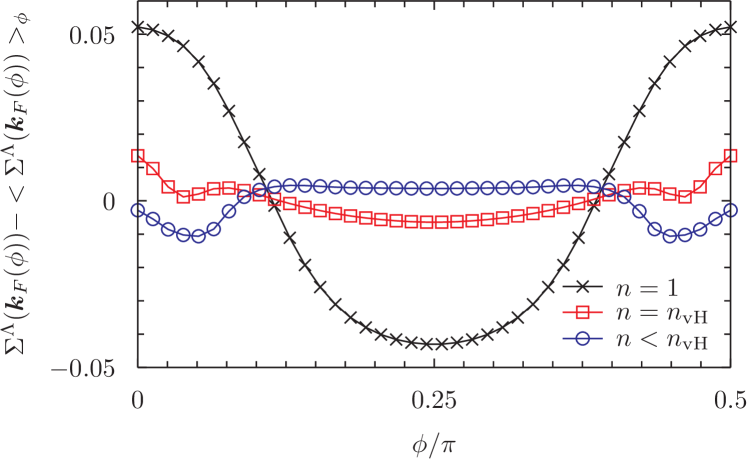
Figure 4: (Color online) Momentum dependence of the self-energy $\Sigma^{\Lambda}(\boldsymbol{k})$ along the Fermi surface in the first quadrant of the Brillouin zone at the end of the flow for $U=3$, $t^{\prime}=-0.2$ and different fillings. The latter and the corresponding critical scales are the same as in Fig. 3. In order to emphasize the momentum dependence, we subtracted the average of $\Sigma^{\Lambda}(\boldsymbol{k})$ over all patches. $\phi=0$ and $\phi=\frac{\pi}{2}$ correspond to the antinodal direction.

The deformation of the Fermi surface as shown in Fig. 3 is caused by the self-energies shown in Fig. 4. This figure shows $\Sigma^{\Lambda}(\boldsymbol{k})$ along the Fermi surface after subtracting the average over all patches in order to highlight the momentum dependence. As expected from the small change of critical scales and Fermi surfaces (see Fig. 1 and 3), at the lower fillings the magnitude of $\Sigma^{\Lambda}(\boldsymbol{k})$ along the Fermi surface is very small. At half-filling, the self-energy is significantly larger and has a more pronounced momentum dependence.

Parametrizing this self-energy in terms of renormalized hopping amplitudes to neighboring lattice sites as in Ref. Giering and Salmhofer, 2012 should yield a very good approximation for all fillings. However, in the one-loop fRG truncation with self-energy feedback Katanin (2004), the scale-derivative of the self-energy also contributes on the right-hand side of the flow equation. As can be seen in Fig. 5, $\frac{d}{d\Lambda}\Sigma^{\Lambda}(\boldsymbol{k})$ for the half-filled system develops a strong dependence on momentum at low scales. A parametrization with a small number of renormalized hopping amplitudes may lead to an underestimation of $\frac{d}{d\Lambda}\Sigma^{\Lambda}(\boldsymbol{k})$ and thus of the impact of fluctuations on the flow in this regime, in particular if the renormalization contributions to the hoppings are determined using Brillouin zone averages. Note that at lower fermionic densities (close to van Hove filling or below), $\frac{d}{d\Lambda}\Sigma^{\Lambda}(\boldsymbol{k})$ remains small and is less important at low scales.

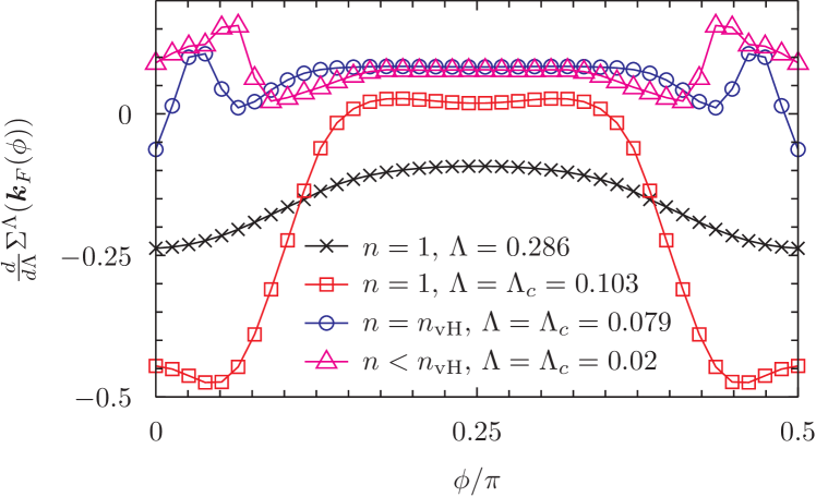
Figure 5: (Color online) Momentum dependence of the scale-derivative of the self-energy $\frac{d}{d\Lambda}\Sigma^{\Lambda}(\boldsymbol{k})$ along the Fermi surface in the first quadrant of the Brillouin zone at the end of the flow for $U=3$, $t^{\prime}=-0.2$ and different fillings. The latter and the corresponding critical scales are the same as in Fig. 3.

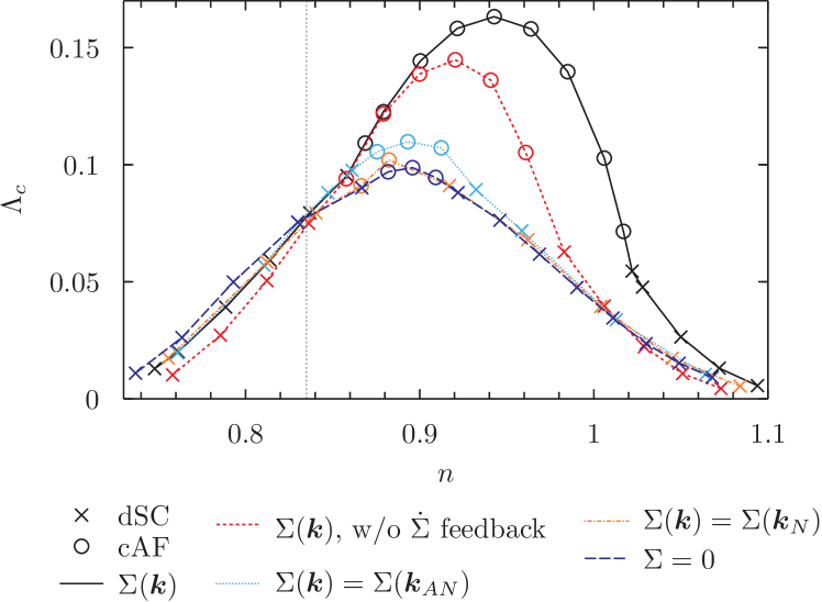
Figure 6: (Color online) Impact of different approximations for the self-energy $\Sigma^{\Lambda}(\boldsymbol{k})$ on the critical scale $\Lambda_{c}$ of fRG flows in static approximation for $U=3$ and $t^{\prime}=-0.2$. Symbols represent the leading instability as in Fig. 1. The different approximations are explained in the text.

The relevance of the momentum dependence of $\Sigma^{\Lambda}(\boldsymbol{k})$ and $\frac{d}{d\Lambda}\Sigma^{\Lambda}(\boldsymbol{k})$ is illustrated in Fig. 6, which shows the critical scales of static one-loop flows using different approximations for the self-energy and its scale-derivative. We show results for $t^{\prime}=-0.2$ in this figure in order to highlight the effect of different approximations, which is somewhat amplified because $U$ is close to the critical value below which no instability to antiferromagnetism appears in the phase diagram when neglecting the momentum dependence of $\Sigma^{\Lambda}$. However, the conclusions for other values of $t^{\prime}$ are qualitatively similar. In the figure, we show results for the approximations mentioned above and in addition for one-loop flows where i) $\Sigma^{\Lambda}(\boldsymbol{k})$ is considered but the feedback of $\frac{d}{d\Lambda}\Sigma^{\Lambda}(\boldsymbol{k})$ to the right-hand side of the flow equation neglected (labeled “$\Sigma(\boldsymbol{k})$, w/o $\dot{\Sigma}$ feedback”), ii) a momentum-independent self-energy is used and evaluated for the Fermi momentum in the antinodal direction closest to the saddle points (labeled “$\Sigma(\boldsymbol{k})=\Sigma(\boldsymbol{k}_{AN})$”) and iii) the same as (ii) but evaluated for a Fermi momentum in the nodal direction (labeled “$\Sigma(\boldsymbol{k})=\Sigma(\boldsymbol{k}_{N})$”). Evaluation of the momentum-independent self-energy in the nodal direction yields critical scales that are almost equal to those that result when the self-energy is neglected completely or evaluated as a Fermi surface average. The reason is that in this case the self-energy flows only weakly at low scales because the nodal points are closer together than $(\pi,\pi)$ and antiferromagnetic fluctuations thus ineffective. Evaluation of the self-energy in the antinodal direction has a somewhat larger effect on critical scales close to van Hove filling. In this case the influence of antiferromagnetic fluctuations is larger and changes in $\Sigma^{\Lambda}$ strongly influence the density of states at the Fermi level. Sufficiently away from van Hove filling, antiferromagnetic fluctuations cease to be effective in renormalizing $\Sigma^{\Lambda}$ in this approximation and the self-energy becomes unimportant. Taking the momentum dependence of $\Sigma^{\Lambda}$ into account but neglecting the feedback of $\dot{\Sigma}^{\Lambda}$, the critical scale is significantly enhanced in a certain density range above van Hove filling, but smaller than with full self-energy feedback. It is interesting to note that not only the deformation of the Fermi surface matters, but that the feedback of $\dot{\Sigma}^{\Lambda}$ also has a sizable impact on critical scales.

III.2 Static one-loop flows and fRG+MF

Former fRG studies, which mainly focused on the parameter regime around van Hove filling, found that the renormalization of the Fermi surface has a small impact on the flow. In the last section we found that taking the fermionic self-energy into account can strongly enhance critical scales close to half-filling. This could be due to an underlying physical mechanism or due to using a different regulator. It is known that critical scales of fRG flows depend to some extent on the employed regularization scheme. An extreme example are forward scattering driven instabilities with $\boldsymbol{q}=\boldsymbol{0}$, which cannot be detected as instabilities of one-loop fRG flows at zero temperature when using a momentum cutoff Halboth and Metzner (2000b), but which show up when using frequency Husemann and Salmhofer (2009) or temperature Honerkamp and Salmhofer (2001) cutoff schemes. It would be interesting to better understand the origin of the larger impact of the self-energy found in the last section.

For this purpose we use a combination of fRG and mean-field theory (MF) to compute order parameters based on input from fRG flows Reiss et al. (2007); Wang et al. (2014), as order parameters should have a weaker dependence on regularization schemes than critical scales. This approach was already applied to study the competition of superconductivity with commensurate Reiss et al. (2007); Wang et al. (2014) and incommensurate Yamase et al. (2015) antiferromagnetism in the ground state of the two-dimensional Hubbard model. For superconducting ground states, the method yielded superconducting gaps in good agreement with results from one-loop fRG flows into the symmetry broken phase Eberlein and Metzner (2014).

The increase of critical scales discussed in the last section is a consequence of the interplay between Fermi surface deformation and antiferromagnetic fluctuations. We therefore restrict ourselves to the computation of the magnetic phase diagram and consider only gaps due to commensurate antiferromagnetism in the mean-field calculation. Near half-filling and on the electron-doped side this is justified because the antiferromagnetic gap is only weakly affected by coexisting superconducting order Yamase et al. (2015). For simplicity we do not further renormalize the normal self-energy in the mean-field calculation. Changes of the antiferromagnetic gap therefore reflect changes of the vertex and the Fermi surface due to self-energy feedback during the fRG flow. We expect that renormalizing the Fermi surface in the mean-field part of the calculation would further increase antiferromagnetic ordering tendencies.

After stopping the fRG flow at the critical scale $\Lambda_{c}$, which we take as the mean-field scale $\Lambda_{\text{MF}}$, we extract the irreducible vertex $\tilde{U}_{\boldsymbol{k}\boldsymbol{k}^{\prime}}$ in the antiferromagnetic channel with transfer momentum $\boldsymbol{Q}=(\pi,\pi)$ from the full vertex in this channel,

$$U_{\boldsymbol{k}\boldsymbol{k}^{\prime}}=\sum_{\sigma}\epsilon_{\sigma}\Gamma^{(4)\,\Lambda_{\text{MF}}}_{\uparrow\sigma\sigma\uparrow}(k+Q,k^{\prime},k^{\prime}+Q,k)|_{k_{0}=k_{0}^{\prime}=0},$$ (22)

where $Q=(0,\boldsymbol{Q})$ and $\epsilon_{\uparrow}=1$, $\epsilon_{\downarrow}=-1$, via a Bethe-Salpeter-like integral equation,

$$\begin{split}U_{\boldsymbol{k}\boldsymbol{k}^{\prime}}&=\tilde{U}_{\boldsymbol{k}\boldsymbol{k}^{\prime}}+\int_{p_{0}}\int_{\boldsymbol{p}}\tilde{U}_{\boldsymbol{k}\boldsymbol{p}}G^{\Lambda_{\text{MF}}}(p)G^{\Lambda_{\text{MF}}}(p+Q)U_{\boldsymbol{p}\boldsymbol{k}^{\prime}},\end{split}$$ (23)

where $\int_{p_{0}}$ and $\int_{\boldsymbol{p}}$ are shorthands for $\int\negthinspace\frac{dp_{0}}{2\pi}$ and $\int\negthinspace\frac{d^{2}p}{(2\pi)^{2}}$, respectively, and $G^{\Lambda_{\text{MF}}}$ is the fermionic propagator including the self-energy at scale $\Lambda_{\text{MF}}=\Lambda_{c}$. The irreducible vertex is inserted into the antiferromagnetic gap equation

$$A_{\boldsymbol{k}}=\frac{1}{2}\int_{\boldsymbol{k}^{\prime}}\tilde{U}_{\boldsymbol{k}\boldsymbol{k}^{\prime}}\langle m_{\boldsymbol{k}^{\prime}}\rangle,$$ (24)

where $m_{\boldsymbol{k}}=a^{\dagger}_{\boldsymbol{k}\uparrow}a_{\boldsymbol{k}+\boldsymbol{Q}\uparrow}-a^{\dagger}_{\boldsymbol{k}\downarrow}a_{\boldsymbol{k}+\boldsymbol{Q}\downarrow}$ is the staggered magnetization and $a^{(\dagger)}$ are fermionic annihilation (creation) operators. The expectation values are computed using the mean-field Hamiltonian

$$\begin{split}H_{\text{MF}}=&\int_{\boldsymbol{k}}\sum_{\sigma}\bigl{(}\epsilon(\boldsymbol{k})+\Sigma^{\Lambda_{c}}(\boldsymbol{k})\bigr{)}a^{\dagger}_{\boldsymbol{k}\sigma}a_{\boldsymbol{k}\sigma}\\ &+\int_{\boldsymbol{k}}A_{\boldsymbol{k}}(m_{\boldsymbol{k}}-\tfrac{1}{2}\langle m_{\boldsymbol{k}}\rangle).\end{split}$$ (25)

Such an effective Hamiltonian formulation is possible because we use a static approximation. Note that the self-consistency equations are solved at $\Lambda=0$, i. e. in the absence of a regulator.

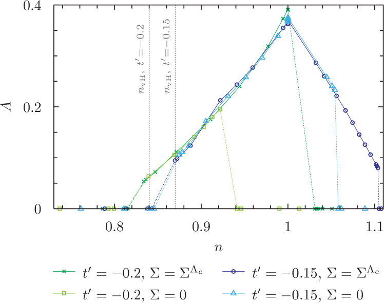
Figure 7: (Color online) Amplitude of the antiferromagnetic gap function for $U=3$ and two values of $t^{\prime}$. The results were obtained as solutions of the gap equation, based on fRG flows in which the normal self-energy was renormalized (labeled “$\Sigma=\Sigma^{\Lambda_{c}}$”) or neglected completely (labeled “$\Sigma=0$”). The normal self-energy was not renormalized in the mean-field calculation. Dashed lines are guides to the eye at first order phase transitions. Dashed grey vertical lines mark van Hove filling.

In Fig. 7 we show the magnetic phase diagram as obtained from solving the gap equation for $U=3$ and two values of $t^{\prime}$, comparing how the renormalization of the self-energy and its feedback in the fRG flow change the magnetic order parameter. The input for the gap equation is obtained (i) from a fRG flow in which the self-energy is neglected completely, $\Sigma=0$, and (ii) from a fRG flow in which a momentum dependent self-energy $\Sigma(\boldsymbol{k})$ is considered. In all cases, the antiferromagnetic order disappears via first-order transitions. The antiferromagnetic gap is almost unchanged where it appears in both approximations. For $t^{\prime}=-0.2$ and $\Sigma=0$, antiferromagnetism exists only close to van Hove filling. Renormalizing the normal self-energy in the fRG flow for this value of $t^{\prime}$, the antiferromagnetic phase gets significantly larger and extends up to half-filling. For $t^{\prime}=-0.15$ and $\Sigma=0$, the antiferromagnetic phase already extends to the electron-doped side. Renormalizing the Fermi surface during the fRG flow leads to an extension of the antiferromagnetic phase and a strong reduction of the first-order transition between the antiferromagnetic and the paramagnetic metal. This shift of phase boundaries and the enlarged antiferromagnetic regimes are the reason for the increase of critical scales in the fRG flow as discussed in the last section. The reduction of the first-order character of the magnetic phase transition for $t^{\prime}=-0.15$ seems to be generic for cases where the antiferromagnetic phase extends beyond half-filling. Note that the first order transitions to metallic states on the hole-doped side are artifacts of our approximation, as they would be preempted by first order transitions to metallic incommensurate antiferromagnetic states Igoshev et al. (2010); Yamase et al. (2015). On the other hand our results suggest that self-energy corrections do not qualitatively modify the findings by Yamase et al. Yamase et al. (2015) as self-energy corrections are of minor importance below and around van Hove filling.

III.3 Dynamic one-loop flows

In this section we briefly discuss what happens if the frequency dependence of the vertex and the self-energy are taken into account as described in Sec. II.3. Our flow equations are very similar to those of Husemann et al. Husemann et al. (2012) and Giering and Salmhofer Giering and Salmhofer (2012). Here we also solve them away from van Hove filling in particular close to half-filling where antiferromagnetic hot spots exist on the Fermi surface.

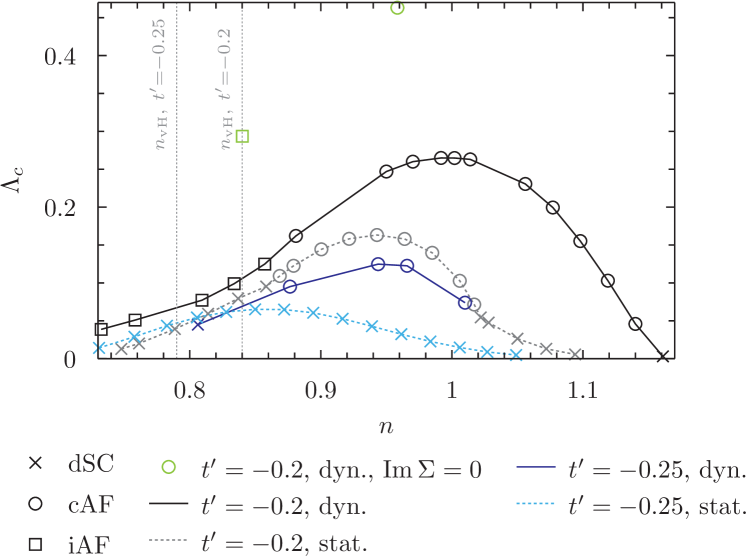
Figure 8: (Color online) Critical scales $\Lambda_{c}$ from dynamic (“dyn.”, full lines) and static (“stat.”, dashed lines) one-loop fRG flows for $U=3$ and different values of $t^{\prime}$. Symbols indicate the leading instability as in Fig. 1. Also shown are a few data points from dynamic one-loop flows in which $\operatorname{Im}\Sigma^{\Lambda}$ was neglected (“$\operatorname{Im}\Sigma=0$”, only symbols). The vertical dashed lines mark van Hove filling.

We do not show results for the frequency dependence of the exchange propagators and the self-energy, as they are qualitatively similar to those in Refs. Husemann et al., 2012; Giering and Salmhofer, 2012. In Fig. 8, we compare critical scales from static and dynamic one-loop flows for $U=3$ and $t^{\prime}=-0.2$ as well as $-0.25$. We observe that taking the frequency dependence of the self-energy and the vertex into account yields larger critical scales and a broader density range with antiferromagnetism as leading instability. For $t^{\prime}=-0.25$, antiferromagnetic instabilities appear, which were not present in the static approximation. The increase of critical scales in comparison to the static approximation seems to be a peculiarity of the chosen regulator and should not be misunderstood in the sense that a frequency dependent vertex and self-energy, and in particular a reduced quasiparticle weight, enhance ordering tendencies. Fluctuation contributions are weighted differently in the static and the dynamic one-loop approximation. Which one yields smaller critical scales depends on the regularization scheme. For a smooth multiplicative frequency regulator Husemann et al. (2012); Giering and Salmhofer (2012) and a sharp multiplicative momentum cutoff Uebelacker and Honerkamp (2012), it was found for the repulsive Hubbard model at van Hove filling that the critical scales were smaller in the dynamic than in the static approximation. For the attractive Hubbard model and the same regulator as employed in this work, the static approximation yielded smaller critical scales and superconducting gaps than the dynamic approximation Eberlein and Metzner (2013). Neglecting the frequency dependence of the self-energy (and thus the renormalization of the quasiparticle weight via $\operatorname{Im}\Sigma$), but taking the frequency dependence of the vertex into account, yields a further increase of critical scales for all regulators. This is shown in Fig. 8 for the regulator used in this work for two fillings. Note that although the critical scales are rather high in this case, they are still significantly smaller than the critical scales of RPA-like flows in which all fluctuation contributions are neglected (in the latter case we obtain $\Lambda_{c}=0.58$ and $0.78$ for $n=0.83$ and $1.07$, respectively).

Computing the self-energy in the $N$-patch approximation allowed us to resolve its frequency dependence and its momentum dependence along the Fermi surface with high resolution. In Fig. 9, we show the variation of the quasiparticle weight

$$Z^{\Lambda}(\boldsymbol{k})=\bigl{(}1-\partial_{k_{0}}\operatorname{Im}\Sigma^{\Lambda}(k_{0},\boldsymbol{k})|_{k_{0}=0}\bigr{)}^{-1}$$ (26)

along the Fermi surface for $U=3$, $t^{\prime}=-0.2$ and various fermionic densities. In all cases shown, the quasiparticle weight is smallest very close to the antiferromagnetic hot spots. At van Hove filling, the minimum is slightly shifted away from the saddle point of the fermionic dispersion because the antiferromagnetic fluctuations are incommensurate at low scales. The quasiparticle weight also shows a sizable anisotropy between the nodal and the antinodal direction, in agreement with former fRG studies for similar parameters Honerkamp and Salmhofer (2003); Uebelacker and Honerkamp (2012). With increasing filling, the anisotropy weakens and the minima shift towards the Brillouin zone diagonal. $Z^{\Lambda}(\boldsymbol{k}_{F})$ being minimal at the hot spots is consistent with the behavior of the spin-fermion model at a spin-density wave quantum critical point with ordering momentum $\boldsymbol{Q}=(\pi,\pi)$ Lee et al. (2013). It is interesting that the quasiparticle weight is largest for $n=1.14$, although the critical scale is lower and the Fermi velocities at the hot spots are slightly more antiparallel than at half-filling.

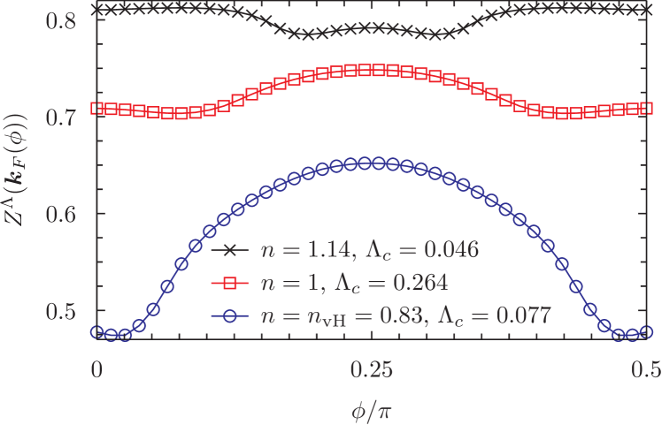
Figure 9: (Color online) Quasiparticle weight $Z^{\Lambda}$ along the Fermi surface at the end of the flow for $U=3$, $t^{\prime}=-0.2$ and various densities. $\phi=0$ and $\pi/2$ denote the antinodal region.

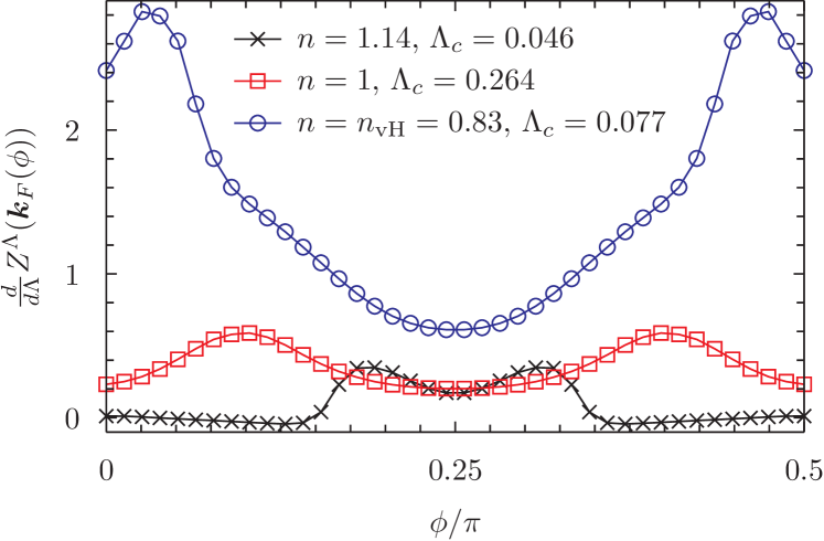
Figure 10: (Color online) Scale-derivative of the quasiparticle weight $\frac{d}{d\Lambda}Z^{\Lambda}$ along the Fermi surface at the end of the flow for $U=3$, $t^{\prime}=-0.2$ and the same densities as in Fig. 9.

The angular dependence of the scale-derivative of the quasiparticle weight is qualitatively similar to that of $Z^{\Lambda}$, as can be seen in Fig. 10. In case the antiferromagnetic fluctuations are commensurate, the maximum is located at the antiferromagnetic hot spots. At van Hove filling, the maximum is shifted slightly away from the saddle points due to incommensurate magnetic fluctuations. Note that a positive $\frac{d}{d\Lambda}Z^{\Lambda}$ yields a reduction of $Z^{\Lambda}$ during the flow.

IV Conclusion

In this paper, we have analyzed the impact of self-energy effects on functional renormalization group flows away from van Hove filling. For the latter filling, which was mostly studied before, our conclusions agree very well with the literature. In particular, fluctuation induced deformations of the Fermi surface have a small impact on the flow. This changes for higher fillings, where antiferromagnetic hot spots exist. In this regime, mostly antiferromagnetic fluctuations lead to a flattening of the Fermi surface, which itself amplifies the magnetic fluctuations. This effect is well known and here we showed that it significantly enhances ordering tendencies to commensurate antiferromagnetism and leads to higher critical scales. Interestingly, for the parameters considered in this work the maximum of critical scales is always shifted towards half-filling.

Using a combination of functional renormalization group and mean-field theory, we showed that self-energy corrections lead to strong shifts of magnetic phase boundaries and can reduce the first order character of antiferromagnetic phase transitions. The former is the underlying reason for the enhanced ordering tendencies and critical scales as found in the renormalization group flow.

Also considering the frequency dependence of the vertex and the self-energy within a dynamic approximation, we found a further increase of critical scales and enlargement of the parameter region with antiferromagnetic order. Note that the critical scales are nevertheless significantly smaller than in an RPA-type approximation where fluctuations are neglected.

On the question whether deformations of the Fermi surface have a qualitative impact on phase diagrams derived from one-loop functional renormalization group flows, our results suggest that they are indeed important close to first order phase transitions with finite ordering wave vectors as in the case of antiferromagnetism, or in the presence of hot spots. For lower electron densities below and around van Hove filling, they seem to be of minor importance.

Appendix A Flow equations for the vertex and the self-energy

In this appendix, we describe the flow equations for the vertex and the self-energy in somewhat more detail. Note that we exploit translation invariance, spin rotation invariance and time reversal symmetry for their derivation.

The flow equation for the effective interaction in the magnetic channel reads

$$\frac{d}{d\Lambda}M^{\Lambda}_{kk^{\prime}}(q)=\frac{1}{2}\int\negthickspace\negthinspace\frac{d^{3}p}{(2\pi)^{3}}\frac{d}{d\Lambda}\bigl{(}G^{\Lambda}(p-\tfrac{q}{2})G^{\Lambda}(p+\tfrac{q}{2})\bigr{)}\Gamma^{(4)\,\Lambda}_{\uparrow\downarrow\uparrow\downarrow}(k+\tfrac{q}{2},p-\tfrac{q}{2},p+\tfrac{q}{2},k-\tfrac{q}{2})\Gamma^{(4)\,\Lambda}_{\downarrow\uparrow\downarrow\uparrow}(k^{\prime}-\tfrac{q}{2},p+\tfrac{q}{2},p-\tfrac{q}{2},k^{\prime}+\tfrac{q}{2}).$$ (27)

Inserting the channel decomposition of the vertex, its component relevant for this flow equation reads

$$\Gamma^{(4)\,\Lambda}_{\uparrow\downarrow\uparrow\downarrow}(k+\tfrac{q}{2},p-\tfrac{q}{2},p+\tfrac{q}{2},k-\tfrac{q}{2})=-U+2M^{\Lambda}_{kp}(q)+M^{\Lambda}_{\frac{k+p-q}{2},\frac{k+p+q}{2}}(p-k)-C^{\Lambda}_{\frac{k+p-q}{2},\frac{k+p+q}{2}}(p-k)-P^{\Lambda}_{\frac{k-p+q}{2},\frac{p-k+q}{2}}(p+k),$$ (28)

where $\Gamma^{(4)\,\Lambda}_{\downarrow\uparrow\downarrow\uparrow}(k^{\prime}-\tfrac{q}{2},p+\tfrac{q}{2},p-\tfrac{q}{2},k^{\prime}+\tfrac{q}{2})=\Gamma^{(4)\,\Lambda}_{\uparrow\downarrow\uparrow\downarrow}(k^{\prime}+\tfrac{q}{2},p-\tfrac{q}{2},p+\tfrac{q}{2},k^{\prime}-\tfrac{q}{2})$ due to symmetries. For the effective interaction in the charge channel, we obtain

$$\begin{split}\frac{d}{d\Lambda}C^{\Lambda}_{kk^{\prime}}(q)=\int\negthickspace\negthinspace\frac{d^{3}p}{(2\pi)^{3}}&\frac{d}{d\Lambda}\bigl{(}G^{\Lambda}(p-\tfrac{q}{2})G^{\Lambda}(p+\tfrac{q}{2})\bigr{)}\Bigl{(}\Gamma^{(4)\,\Lambda}_{\uparrow\uparrow\uparrow\uparrow}(k+\tfrac{q}{2},p-\tfrac{q}{2},p+\tfrac{q}{2},k-\tfrac{q}{2})\Gamma^{(4)\,\Lambda}_{\downarrow\uparrow\uparrow\downarrow}(k^{\prime}-\tfrac{q}{2},p+\tfrac{q}{2},p-\tfrac{q}{2},k^{\prime}+\tfrac{q}{2})\\ &+\Gamma^{(4)\,\Lambda}_{\uparrow\downarrow\downarrow\uparrow}(k+\tfrac{q}{2},p-\tfrac{q}{2},p+\tfrac{q}{2},k-\tfrac{q}{2})\Gamma^{(4)\,\Lambda}_{\downarrow\downarrow\downarrow\downarrow}(k^{\prime}-\tfrac{q}{2},p+\tfrac{q}{2},p-\tfrac{q}{2},k^{\prime}+\tfrac{q}{2})\Bigr{)}+\frac{d}{d\Lambda}M^{\Lambda}_{kk^{\prime}}(q),\end{split}$$ (29)

where

$$\begin{split}\Gamma^{(4)\,\Lambda}_{\uparrow\uparrow\uparrow\uparrow}(k+\tfrac{q}{2},p-\tfrac{q}{2},p+\tfrac{q}{2},k-\tfrac{q}{2})=&M^{\Lambda}_{kp}(q)+C^{\Lambda}_{kp}(q)-M^{\Lambda}_{\frac{k+p-q}{2},\frac{k+p+q}{2}}(p-k)-C^{\Lambda}_{\frac{k+p-q}{2},\frac{k+p+q}{2}}(p-k)\\ &+P^{\Lambda}_{\frac{k-p+q}{2},\frac{k-p-q}{2}}(k+p)-P^{\Lambda}_{\frac{k-p+q}{2},-\frac{k-p-q}{2}}(k+p),\end{split}$$ (30)

$$\Gamma^{(4)\,\Lambda}_{\uparrow\downarrow\downarrow\uparrow}(k+\tfrac{q}{2},p-\tfrac{q}{2},p+\tfrac{q}{2},k-\tfrac{q}{2})=U+C^{\Lambda}_{kp}(q)-M^{\Lambda}_{kp}(q)-2M^{\Lambda}_{\frac{k+p-q}{2},\frac{k+p+q}{2}}(p-k)+P^{\Lambda}_{\frac{k-p+q}{2},\frac{k-p-q}{2}}(p+k).$$ (31)

Symmetries allow to rewrite $\Gamma^{(4)\,\Lambda}_{\downarrow\uparrow\uparrow\downarrow}(k^{\prime}-\tfrac{q}{2},p+\tfrac{q}{2},p-\tfrac{q}{2},k^{\prime}+\tfrac{q}{2})=\Gamma^{(4)\,\Lambda}_{\uparrow\downarrow\downarrow\uparrow}(k^{\prime}+\tfrac{q}{2},p-\tfrac{q}{2},p+\tfrac{q}{2},k^{\prime}-\tfrac{q}{2})$ and $\Gamma^{(4)\,\Lambda}_{\downarrow\downarrow\downarrow\downarrow}(k^{\prime}-\tfrac{q}{2},p+\tfrac{q}{2},p-\tfrac{q}{2},k^{\prime}+\tfrac{q}{2})=\Gamma^{(4)\,\Lambda}_{\uparrow\uparrow\uparrow\uparrow}(k^{\prime}+\tfrac{q}{2},p-\tfrac{q}{2},p+\tfrac{q}{2},k^{\prime}-\tfrac{q}{2})$. Note that the contributions of the particle-particle channel in Eq. (30) vanish in case only singlet pairing fluctuations are considered.

The flow of the effective interaction in the particle-particle channel is determined by the flow equation

$$\begin{split}\frac{d}{d\Lambda}P^{\Lambda}_{kk^{\prime}}(q)=-\frac{1}{2}\int\negthickspace\negthinspace\frac{d^{3}p}{(2\pi)^{3}}&\frac{d}{d\Lambda}\bigl{(}G^{\Lambda}(\tfrac{q}{2}-p)G^{\Lambda}(\tfrac{q}{2}+p)\bigr{)}\Bigl{(}\Gamma^{(4)\,\Lambda}_{\uparrow\downarrow\downarrow\uparrow}(k+\tfrac{q}{2},\tfrac{q}{2}-k,\tfrac{q}{2}-p,\tfrac{q}{2}+p)\Gamma^{(4)\,\Lambda}_{\uparrow\downarrow\downarrow\uparrow}(\tfrac{q}{2}+p,\tfrac{q}{2}-p,\tfrac{q}{2}-k^{\prime},\tfrac{q}{2}+k^{\prime})\\ &+\Gamma^{(4)\,\Lambda}_{\uparrow\downarrow\uparrow\downarrow}(\tfrac{q}{2}+k,\tfrac{q}{2}-k,\tfrac{q}{2}-p,\tfrac{q}{2}+p)\Gamma^{(4)\,\Lambda}_{\downarrow\uparrow\downarrow\uparrow}(\tfrac{q}{2}+p,\tfrac{q}{2}-p,\tfrac{q}{2}-k^{\prime},\tfrac{q}{2}+k^{\prime})\Bigr{)},\end{split}$$ (32)

where

$$\begin{split}\Gamma^{(4)\,\Lambda}_{\uparrow\downarrow\downarrow\uparrow}(\tfrac{q}{2}+k,\tfrac{q}{2}-k,\tfrac{q}{2}-p,\tfrac{q}{2}+p)=&U+P^{\Lambda}_{kp}(q)-2M^{\Lambda}_{\frac{p-k+q}{2},\frac{k-p+q}{2}}(-k-p)+C^{\Lambda}_{\frac{k+p+q}{2},\frac{q-k-p}{2}}(k-p)\\ &-M^{\Lambda}_{\frac{k+p+q}{2},\frac{q-k-p}{2}}(k-p),\end{split}$$ (33)

$$\begin{split}\Gamma^{(4)\,\Lambda}_{\uparrow\downarrow\uparrow\downarrow}(\tfrac{q}{2}+k,\tfrac{q}{2}-k,\tfrac{q}{2}-p,\tfrac{q}{2}+p)=&-U-P^{\Lambda}_{k,-p}(q)+2M^{\Lambda}_{\frac{k+p+q}{2},\frac{q-k-p}{2}}(k-p)-C^{\Lambda}_{\frac{p-k+q}{2},\frac{q+k-p}{2}}(-k-p)\\ &+M^{\Lambda}_{\frac{p-k+q}{2},\frac{q+k-p}{2}}(-k-p)\end{split}$$ (34)

Note that due to symmetries, $\Gamma^{(4)\,\Lambda}_{\uparrow\downarrow\downarrow\uparrow}(\tfrac{q}{2}+p,\tfrac{q}{2}-p,\tfrac{q}{2}-k^{\prime},\tfrac{q}{2}+k^{\prime})=\Gamma^{(4)\,\Lambda}_{\uparrow\downarrow\downarrow\uparrow}(\tfrac{q}{2}+k^{\prime},\tfrac{q}{2}-k^{\prime},\tfrac{q}{2}-p,\tfrac{q}{2}+p)$ and $\Gamma^{(4)\,\Lambda}_{\downarrow\uparrow\downarrow\uparrow}(\tfrac{q}{2}+p,\tfrac{q}{2}-p,\tfrac{q}{2}-k^{\prime},\tfrac{q}{2}+k^{\prime})=\Gamma^{(4)\,\Lambda}_{\uparrow\downarrow\uparrow\downarrow}(\tfrac{q}{2}+k^{\prime},\tfrac{q}{2}-k^{\prime},\tfrac{q}{2}-p,\tfrac{q}{2}+p)$. As we neglect triplet pairing fluctuations, it is useful to work with a flow equation for the effective interaction in the singlet particle-particle channel, which is given by

$$\begin{split}\frac{d}{d\Lambda}&P^{S,\Lambda}_{kk^{\prime}}(q)=\frac{1}{2}\Bigl{(}\frac{d}{d\Lambda}P^{\Lambda}_{kk^{\prime}}(q)+\frac{d}{d\Lambda}P^{\Lambda}_{k,-k^{\prime}}(q)\Bigr{)}\\ =&-\frac{1}{4}\int\negthickspace\negthinspace\frac{d^{3}p}{(2\pi)^{3}}\frac{d}{d\Lambda}\bigl{(}G^{\Lambda}(\tfrac{q}{2}-p)G^{\Lambda}(\tfrac{q}{2}+p)\bigr{)}\Bigl{(}\Gamma^{(4)\,\Lambda}_{\uparrow\downarrow\downarrow\uparrow}(\tfrac{q}{2}+k,\tfrac{q}{2}-k,\tfrac{q}{2}-p,\tfrac{q}{2}+p)-\Gamma^{(4)\,\Lambda}_{\uparrow\downarrow\uparrow\downarrow}(\tfrac{q}{2}+k,\tfrac{q}{2}-k,\tfrac{q}{2}-p,\tfrac{q}{2}+p)\Bigr{)}\\ &\quad\times\Bigl{(}\Gamma^{(4)\,\Lambda}_{\uparrow\downarrow\downarrow\uparrow}(\tfrac{q}{2}+p,\tfrac{q}{2}-p,\tfrac{q}{2}-k^{\prime},\tfrac{q}{2}+k^{\prime})-\Gamma^{(4)\,\Lambda}_{\uparrow\downarrow\uparrow\downarrow}(\tfrac{q}{2}+p,\tfrac{q}{2}-p,\tfrac{q}{2}-k^{\prime},\tfrac{q}{2}+k^{\prime})\Bigr{)}.\end{split}$$ (35)

These flow equations were evaluated within the approximation scheme described in Sec. II.3 and Appendix B. As we do not renormalize the fermion-boson vertices, we set the external fermionic frequencies to zero, $k_{0}=k_{0}^{\prime}=0$. In order to obtain flow equations for the bosonic exchange propagators, we project the flow equations for the coupling functions by averaging external fermionic momenta $\boldsymbol{k}$ and $\boldsymbol{k}^{\prime}$ over the Fermi surface, as described in Ref. Eberlein and Metzner, 2013.

The flow equation for the self-energy (7) reads

$$\frac{d}{d\Lambda}\Sigma^{\Lambda}(k)=\int\negthickspace\negthinspace\frac{d^{3}p}{(2\pi)^{3}}\bigl{(}\Gamma^{(4)\,\Lambda}_{\uparrow\uparrow\uparrow\uparrow}(k,p,p,k)+\Gamma^{(4)\,\Lambda}_{\uparrow\downarrow\downarrow\uparrow}(k,p,p,k)\bigr{)}S^{\Lambda}(p),$$ (36)

where the relevant components of the vertex are given by Eqs. (30) and (31) with $q=0$.

Appendix B Some details of numerical implementation

In the dynamic approximation, the exchange propagators depend on frequency and momentum $q=(q_{0},\boldsymbol{q})$. These dependences are discretized on a three-dimensional grid. The momentum dependence is described with two grids in polar coordinates around $\boldsymbol{q}=\boldsymbol{0}$ and $\boldsymbol{q}=\boldsymbol{\pi}$, with an increased density of grid points around these momenta, similarly to the grid used in Ref. Husemann and Salmhofer, 2009. The angular dependence is discretized using 3 - 7 angles in the first octant of the Brillouin zone, which is sufficient due to lattice symmetries, and 20 - 40 points for the radial dependence. The number of grid points was chosen higher in channels in which the effective interaction became large at low scales (for example the magnetic channel with momenta close to $\boldsymbol{q}\approx\boldsymbol{\pi}$ or the $d$-wave pairing channel with momenta close to $\boldsymbol{q}\approx\boldsymbol{0}$), while less points were used for effective interactions that remained small during the flow (for example $s$-wave charge density wave fluctuations with $\boldsymbol{q}\approx\boldsymbol{0}$). In case the leading instability was towards incommensurate states, we adjusted the momentum grid in such a way that the density of grid points is higher close to the anticipated position of the incommensurate peaks. The frequency dependence is discretized on a non-equidistant grid with typically 30 - 40 frequencies between $q_{0,\text{min}}=0$ and $q_{0,\text{max}}=250$, where the density of grid points decreases towards higher frequencies. Linear interpolation is used for intermediate momenta and frequencies. We neglect the dependence of the effective interactions on the fermionic relative frequencies $k_{0}$, $k_{0}^{\prime}$, which turned out to have a small impact on critical scales Giering and Salmhofer (2012); Eberlein and Metzner (2013). The flow equations are evaluated for $k_{0}=k_{0}^{\prime}=0$, which allows to capture the “bosonic” features in the frequency dependence of the vertex Rohringer et al. (2012) at small frequencies. In the static approximation, we neglect the dependence on $q_{0}$ and evaluate all effective interactions for $q_{0}=0$. The exchange propagators are then discretized on a two-dimensional grid and the numerical effort for solving the flow equations is significantly reduced.

These approximations transform the functional flow equations into a system of nonlinear ordinary differential equations. The coefficients on the right hand sides are given by three-dimensional integrals over loop momenta and frequencies in the dynamic approximation. In the static approximation all frequency integrals are solved analytically and only two-dimensional integrals have to be computed. The integrals are computed numerically with an adaptive algorithm with absolute and relative precision of $10^{-5}$ and $10^{-3}$, respectively. The flow equations were solved numerically with an adaptive fifth-order Runge-Kutta routine Gough (2009) with absolute and relative accuracy goals of $10^{-3}$. The numerical solution was started at a high scale $\Lambda_{0}=100$, where the initial conditions can be computed in second-order perturbation theory.

References

- Scalapino (2012) D. J. Scalapino, Rev. Mod. Phys. 84, 1383 (2012).
- LeBlanc et al. (2015) J. P. F. LeBlanc, A. E. Antipov, F. Becca, I. W. Bulik, G. K.-L. Chan, C.-M. Chung, Y. Deng, M. Ferrero, T. M. Henderson, C. A. Jiménez-Hoyos, E. Kozik, X.-W. Liu, A. J. Millis, N. V. Prokof’ev, M. Qin, G. E. Scuseria, H. Shi, B. V. Svistunov, L. F. Tocchio, I. S. Tupitsyn, S. R. White, S. Zhang, B.-X. Zheng, Z. Zhu, and E. Gull (Simons Collaboration on the Many-Electron Problem), Phys. Rev. X 5, 041041 (2015).
- Wetterich (1993) C. Wetterich, Phys. Lett. B 301, 90 (1993).
- Salmhofer and Honerkamp (2001) M. Salmhofer and C. Honerkamp, Prog. Theor. Phys. 105, 1 (2001).
- Metzner et al. (2012) W. Metzner, M. Salmhofer, C. Honerkamp, V. Meden, and K. Schönhammer, Rev. Mod. Phys. 84, 299 (2012).
- Friederich et al. (2011) S. Friederich, H. C. Krahl, and C. Wetterich, Phys. Rev. B 83, 155125 (2011).
- Eberlein and Metzner (2014) A. Eberlein and W. Metzner, Phys. Rev. B 89, 035126 (2014).
- Machado and Dupuis (2010) T. Machado and N. Dupuis, Phys. Rev. E 82, 041128 (2010).
- Taranto et al. (2014) C. Taranto, S. Andergassen, J. Bauer, K. Held, A. Katanin, W. Metzner, G. Rohringer, and A. Toschi, Phys. Rev. Lett. 112, 196402 (2014).
- Wentzell et al. (2015) N. Wentzell, C. Taranto, A. Katanin, A. Toschi, and S. Andergassen, Phys. Rev. B 91, 045120 (2015).
- Katanin (2004) A. A. Katanin, Phys. Rev. B 70, 115109 (2004).
- Honerkamp et al. (2001) C. Honerkamp, M. Salmhofer, N. Furukawa, and T. M. Rice, Phys. Rev. B 63, 035109 (2001).
- Igoshev et al. (2011) P. A. Igoshev, V. Y. Irkhin, and A. A. Katanin, Phys. Rev. B 83, 245118 (2011).
- Husemann et al. (2012) C. Husemann, K.-U. Giering, and M. Salmhofer, Phys. Rev. B 85, 075121 (2012).
- Giering and Salmhofer (2012) K.-U. Giering and M. Salmhofer, Phys. Rev. B 86, 245122 (2012).
- Platt et al. (2013) C. Platt, W. Hanke, and R. Thomale, Adv. Phys. 62, 453 (2013).
- Reiss et al. (2007) J. Reiss, D. Rohe, and W. Metzner, Phys. Rev. B 75, 075110 (2007).
- Wang et al. (2014) J. Wang, A. Eberlein, and W. Metzner, Phys. Rev. B 89, 121116 (2014).
- Berges et al. (2002) J. Berges, N. Tetradis, and C. Wetterich, Phys. Rep. 363, 223 (2002).
- Kopietz et al. (2010) P. Kopietz, L. Bartosch, and F. Schütz, Introduction to the Functional Renormalization Group, Lecture Notes in Physics, Vol. 798 (Springer, 2010).
- Eberlein and Metzner (2013) A. Eberlein and W. Metzner, Phys. Rev. B 87, 174523 (2013).
- Eberlein (2014) A. Eberlein, Phys. Rev. B 90, 115125 (2014).
- Maier et al. (2014) S. A. Maier, A. Eberlein, and C. Honerkamp, Phys. Rev. B 90, 035140 (2014).
- Karrasch et al. (2008) C. Karrasch, R. Hedden, R. Peters, T. Pruschke, K. Schonhammer, and V. Meden, J. Phys.: Condens. Matter 20, 345205 (2008).
- Husemann and Salmhofer (2009) C. Husemann and M. Salmhofer, Phys. Rev. B 79, 195125 (2009).
- Zanchi and Schulz (2000) D. Zanchi and H. J. Schulz, Phys. Rev. B 61, 13609 (2000).
- Halboth and Metzner (2000a) C. J. Halboth and W. Metzner, Phys. Rev. Lett. 85, 5162 (2000a).
- Husemann and Metzner (2012) C. Husemann and W. Metzner, Phys. Rev. B 86, 085113 (2012).
- Sachdev and La Placa (2013) S. Sachdev and R. La Placa, Phys. Rev. Lett. 111, 027202 (2013).
- Meier et al. (2014) H. Meier, C. Pépin, M. Einenkel, and K. B. Efetov, Phys. Rev. B 89, 195115 (2014).
- Neumayr and Metzner (2003) A. Neumayr and W. Metzner, Phys. Rev. B 67, 035112 (2003).
- Abanov and Chubukov (2000) A. Abanov and A. V. Chubukov, Phys. Rev. Lett. 84, 5608 (2000).
- Metlitski and Sachdev (2010) M. A. Metlitski and S. Sachdev, Phys. Rev. B 82, 075128 (2010).
- Halboth and Metzner (2000b) C. J. Halboth and W. Metzner, Phys. Rev. B 61, 7364 (2000b).
- Honerkamp and Salmhofer (2001) C. Honerkamp and M. Salmhofer, Phys. Rev. B 64, 184516 (2001).
- Yamase et al. (2015) H. Yamase, A. Eberlein, and W. Metzner, ArXiv e-prints (2015), arXiv:1507.00560 [cond-mat.str-el] .
- Igoshev et al. (2010) P. A. Igoshev, M. A. Timirgazin, A. A. Katanin, A. K. Arzhnikov, and V. Y. Irkhin, Phys. Rev. B 81, 094407 (2010).
- Uebelacker and Honerkamp (2012) S. Uebelacker and C. Honerkamp, Phys. Rev. B 86, 235140 (2012).
- Honerkamp and Salmhofer (2003) C. Honerkamp and M. Salmhofer, Phys. Rev. B 67, 174504 (2003).
- Lee et al. (2013) J. Lee, P. Strack, and S. Sachdev, Phys. Rev. B 87, 045104 (2013).
- Rohringer et al. (2012) G. Rohringer, A. Valli, and A. Toschi, Phys. Rev. B 86, 125114 (2012).
- Gough (2009) B. Gough, GNU Scientific Library: Reference Manual, A GNU manual (Network Theory Limited, 2009).