Efficient estimators for likelihood ratio sensitivity indices of complex stochastic dynamics

Abstract

We demonstrate that centered likelihood ratio estimators for the sensitivity indices of complex stochastic dynamics are highly efficient with low, constant in time variance and consequently they are suitable for sensitivity analysis in long-time and steady-state regimes. These estimators rely on a new covariance formulation of the likelihood ratio that includes as a submatrix a Fisher Information Matrix for stochastic dynamics and can also be used for fast screening of insensitive parameters and parameter combinations. The proposed methods are applicable to broad classes of stochastic dynamics such as chemical reaction networks, Langevin-type equations and stochastic models in finance, including systems with a high dimensional parameter space and/or disparate decorrelation times between different observables. Furthermore, they are simple to implement as a standard observable in any existing simulation algorithms without additional modifications.

1 Introduction

In this paper we show that centered ergodic likelihood ratio sensitivity indices give rise to corresponding estimators which are: (a) highly efficient in the sense that they have low, constant in time variance; hence, they provide reliable sensitivity analysis at long-time and steady-state regimes; (b) unsupervised, i.e., they do not require keeping track of the, possibly disparate and sometimes hard to compute, decorrelation times of state variables and observables; (c) widely applicable, for instance to (bio)chemical reaction networks, kinetic Monte Carlo and stochastic differential equations such as (possibly non-reversible) Langevin molecular dynamics or stochastic models in finance; (d) gradient-free, i.e., all sensitivities are computed in the course of a single simulation, hence they are applicable to systems with a very high dimensional parameter space; (e) non-intrusive in the sense that they do not require modifications to existing simulation algorithms since they are simple to implement as a standard observable. We demonstrate these points by implementing the method in complex reaction networks and stochastic differential equations and discuss variance reduction and applicability of the estimators considered. Finally, we compare these likelihood ratio estimators to finite difference methods with stochastic coupling, including a proposed, highly efficient ergodic stochastic coupling estimator.

A centered ergodic likelihood ratio (LR) estimator (14) was proposed originally in [12], Section 5, see also Ch. VII, Remark 4.4 [5], where it is derived as an optimized, reduced variance–in the sense of control variates–alternative to the standard LR. Centered LR estimators with decorrelation-length truncation to reduce variance were also considered in [25]. The centered ergodic LR of [5] was also used very recently in the sensitivity analysis of two-scale reaction networks[14].

The novelty in our paper is two-fold. First, we demonstrate through a combination of examples and theoretical analysis that centered ergodic LR (14) is an attractive practical tool for sensitivity analysis of complex stochastic at long-time and steady-state regimes with the features (a-e) above; we also show that it compares favorably to existing sensitivity estimators [1, 5, 25], and at the same time it is straightforward to implement computationally. Second, we show that the centered ergodic LR (14) is an off-diagonal submatrix of a new Covariance Likelihood Ratio estimator (16) between observables and the score of the process. The proposed Covariance LR yields simultaneously parameter screening, (17), and sensitivities, (14). In particular, the Covariance LR includes as a submatrix a Fisher Information Matrix for stochastic dynamics which, as shown recently [3, 6], can also be used for fast screening of insensitive parameters and parameter combinations.

2 Estimators of Sensitivity Indices

In the following we will use $\mathbb{E}_{P^{\theta}_{0:T}}\left[F(X_{0:T})\right]$ to denote the expected value of an observable $F=F(X_{0:T})$ which may depend on the stochastic process $X_{0:T}:=\big{\{}X_{t}\big{\}}_{t=0}^{T}$ in the time interval $[0,T]$. The probability distribution of $X_{0:T}$ in the sample space of time series–referred as the path space–is denoted by $P^{\theta}_{0:T}$. We use the notation $\langle\cdot\rangle_{\mu}$ for sample averages over independent identically distributed samples from probability measure $\mu$, e.g.,

$$\left\langle F(X_{0:T})\right\rangle_{P^{\theta}_{0:T}}=\frac{1}{M}\sum_{k=1}^{M}F\big{(}X^{(k)}_{0:T}\big{)},$$ (1)

where $X^{(k)}_{0:T}$ are i.i.d. time series sample from $P^{\theta}_{0:T}$. If $f=f(X_{t})$ is an observable depending on the process at a single instance of time, we then denote the ergodic average of the observable $f$ by

$$\bar{f}(X_{0:T})=\frac{1}{T}\int_{t=0}^{T}f(X_{t})\,dt\,.$$ (2)

The gradient with respect to a parameter vector $\theta$,

$$\nabla_{\theta}\,\mathbb{E}_{P^{\theta}_{0:T}}\left[F(X_{0:T})\right]\,,$$

is known as a sensitivity index, and each one of the partial derivatives can be estimated by various estimators. Next, we divide estimators for such sensitivity indices into two classes. First, sensitivity estimators for observables $f=f(X_{T})$ which depend on the process at a fixed instance in time $T$ such as

$$\frac{\partial}{\partial\theta_{k}}\mathbb{E}_{P^{\theta}_{0:T}}\left[f(X_{T})\right]\,.$$ (3)

Second, we consider sensitivity indices for observables $F=F(X_{0:T})$ that depend on the entire path, in particular for the ergodic averages $\bar{f}(X_{0:T})$ given in (2), namely

$$\frac{\partial}{\partial\theta_{k}}\mathbb{E}_{P^{\theta}_{0:T}}\left[\bar{f}(X_{0:T})\right]\,.$$ (4)

Remark: For long times $T\gg 1$ the two estimators (3) and (4) are expected to become identical, at least for systems with ergodic behavior since in this case (see for instance [17], Chapter 1),

$$\mathbb{E}_{\mu}\left[f(X_{\infty})\right]=\lim_{T\to\infty}\mathbb{E}_{P^{\theta}_{0:T}}\left[f(X_{T})\right]=\lim_{T\to\infty}\mathbb{E}_{P^{\theta}_{0:T}}\left[\bar{f}(X_{0:T})\right]\,,$$ (5)

where $\mu$ denotes the steady state distribution of the stochastic dynamics $X=X_{T}$; here the random variable corresponding to the steady state $\mu$ is denoted by $X_{\infty}$. The rigorous proof of the asymptotic equivalence of (3) and (4) relies on the use of Lyapunov functionals, [13, 4] and is beyond the scope of this paper. However this asymptotic equivalence for $T\gg 1$ suggests that both classes of estimators can, in theory, be used for the sensitivity analysis of ergodic stochastic dynamics at long times. In the remaining of the paper we discuss these points in more detail, see for example the results summarized in Figure 3.

2.1 Estimators for single-time observables

First we consider a centered finite difference approximation of the sensitivity index (3), namely

Estimator $I_{1}$: (Finite Difference with Stochastic Coupling (CFD)) [1]

$$\frac{\partial}{\partial\theta_{k}}\mathbb{E}_{P^{\theta}_{0:T}}\left[f(X_{T})\right]\approx\frac{\mathbb{E}_{P^{\theta+\varepsilon_{k}}_{0:T}}\left[f(X_{T})\right]-\mathbb{E}_{P^{\theta-\varepsilon_{k}}_{0:T}}\left[f(X_{T})\right]}{2\varepsilon}\,,$$ (6)

where $\varepsilon_{k}=\varepsilon e_{k}$ and $e_{k}$ is a vector with $1$ in the $k$-th position and $0$ in all other places. The two processes involved in the finite difference scheme are usually stochastically coupled in order to minimize the variance of the underlying estimator, [1], see also [2] for an approach that optimizes the variance reduction. For this reason, these sensitivity indices are known as Coupling Finite Difference (CFD) estimators, [1]. We will refer to the corresponding estimator as $I_{1}$:

$$I_{1}=\frac{1}{2\epsilon}\left[\left\langle{f(X_{T})}\right\rangle_{P^{\theta+\varepsilon_{k}}_{0:T}}-\left\langle{f(X_{T})}\right\rangle_{P^{\theta-\varepsilon_{k}}_{0:T}}\right]\,.$$ (7)

On the other hand, for any single-time observable $f(X_{T})$, the sensitivity index, under reasonably general conditions, can be written as an observable itself,

$$\nabla_{\theta}\,\mathbb{E}_{P^{\theta}_{0:T}}\left[f(X_{T})\right]\,=\,\mathbb{E}_{P^{\theta}_{0:T}}\left[f(X_{T})\,W^{\theta}(X_{0:T})\right]\,,$$ (8)

which depend on the entire path but which can be evaluated exactly with Monte Carlo sampling. The weight $W^{\theta}$ is known as the score (process) with available analytical expressions for stochastic differential equations in [7] (Proposition 3.1) and discrete and continuous Markov Chains in [5] (Ch. VII Sec. 4); there are also extensions to more general Ito-Levy processes [4]. We refer to the Appendix for the formulas for the weights $W^{\theta}$ for each case discussed here. As a consequence of the exact formulas for $W^{\theta}$, (8) gives rise to Likelihood Ratio (LR) type estimators for $\nabla_{\theta}\mathbb{E}_{P^{\theta}_{0:T}}\left[f(X_{0:T})\right]$:

Estimator $I_{2}$: (Likelihood Ratio) [11]

$$I_{2}=\left\langle{f(X_{T})\;W^{\theta}(X_{0:T})}\right\rangle_{P^{\theta}_{0:T}}.$$ (9)

The ergodic average version of $I_{2}$ in analogy to (4) is denoted by $I_{3}$ and will be discussed in the next subsection. Finally, an additional Likelihood Ratio (LR) estimator results from the truncation of (9) beyond the decorrelation length $T_{d}$ of the process:

Estimator $I_{4}$: (truncated Likelihood Ratio) [25],

$$I_{4}=\left\langle f(X_{T})\left(W^{\theta}(X_{0:T})-W^{\theta}(X_{0:T-T_{d}})\right)\right\rangle_{P^{\theta}_{0:T}}=\left\langle f(X_{T})W^{\theta}(X_{T-T_{d}:T})\right\rangle_{P^{\theta}_{0:T}},$$ (10)

assuming the decorrelation time $T_{d}$ is known, [25].

2.2 Estimators for path-space and ergodic observables

Here we consider sensitivity indices for observables that depend on the entire path, and in particular for ergodic averages $\bar{f}(X_{0:T})$ of observables $f$ such as (2). First we consider the averaged version of the coupled finite difference estimator $I_{1}$:

Estimator $I_{5}$: (Ergodic Finite Difference with Stochastic Coupling)

$$I_{5}=\frac{1}{2\epsilon T}\int_{0}^{T}\Big{[}\left\langle{f(X_{t})}\right\rangle_{P^{\theta+\varepsilon_{k}}_{0:t}}-\left\langle{f(X_{t})}\right\rangle_{P^{\theta-\varepsilon_{k}}_{0:t}}\Big{]}dt\,\,=\,\frac{1}{2\epsilon}\Big{[}\left\langle{\bar{f}(X_{0:T})}\right\rangle_{P^{\theta+\varepsilon_{k}}_{0:T}}-\left\langle{\bar{f}(X_{0:T})}\right\rangle_{P^{\theta-\varepsilon_{k}}_{0:T}}\Big{]}\,.$$ (11)

Next we return to the ergodic version of the LR estimator $I_{2}$. Indeed, for a path-dependent observable $\bar{f}(X_{0:T})$, the sensitivity index $\nabla_{\theta}\mathbb{E}_{P^{\theta}_{0:T}}\left[\bar{f}(X_{0:T})\right]$ can also be written as an observable itself, similarly to (8),

$$\nabla_{\theta}\,\mathbb{E}_{P^{\theta}_{0:T}}\left[\bar{f}(X_{0:T})\right]\,=\,\mathbb{E}_{P^{\theta}_{0:T}}\left[\bar{f}(X_{0:T})\,W^{\theta}(X_{0:T})\right]\,,$$ (12)

hence the sensitivity index can be evaluated with Monte Carlo sampling using the estimator $I_{3}$:

Estimator $I_{3}$: (Ergodic Likelihood Ratio) [12]

$$I_{3}=\left\langle{\bar{f}(X_{0:T})\;W^{\theta}(X_{0:T})}\right\rangle_{P^{\theta}_{0:T}}.$$ (13)

Since the score process has mean $0$, $\mathbb{E}_{P^{\theta}_{0:T}}\left[W^{\theta}(X_{0:T})\right]=0$, each of the estimators $I_{2},I_{3}$ and $I_{4}$ has a centered version where the mean is subtracted from the observable. The centered estimators will denoted by $\bar{I}_{2},\bar{I}_{3}$ and $\bar{I}_{4}$. In particular we will focus our attention on $\bar{I}_{3}$ since it will be shown to be the most efficient and easy to implement:

Estimator $\bar{I}_{3}$: (Centered Ergodic Likelihood Ratio)

$$\bar{I}_{3}=\left\langle{\Big{(}\bar{f}(X_{0:T})-\left\langle{\bar{f}(X_{0:T})}\right\rangle\Big{)}W^{\theta}(X_{0:T})}\right\rangle\,.$$ (14)

Note that $\bar{I}_{3}$ can be derived by variance minimization through a controlled variates approach [5], using that $\mathbb{E}_{P^{\theta}_{0:T}}\left[W^{\theta}(X_{0:T})\right]=0$.

In this paper we compare the estimator $\bar{I}_{3}$ to the standard LR estimators $I_{2}$ and $\bar{I}_{2}$ [11], as well as the coupled finite difference method $I_{1}$ [1] and $I_{5}$ in order to have a benchmark comparison with a highly efficient, low variance method [23, 22]. We also consider the truncated LR $\bar{I}_{4}$ which–like $\bar{I}_{3}$ –provides a gradient-free, low variance method for sensitivity analysis at stationarity, although it relies on the accurate calculation of decorrelation times $T_{d}=T_{d}(f)$ in (10) for all observables $f$ of interest. We do not compare our estimators with pathwise methods [21, 27], since they may require the construction of an auxiliary process [27], which in turn imposes an additional programming overhead for existing simulators.

2.3 Covariance LR Estimator and Sensitivity Screening

As noted earlier that the centered ergodic likelihood ratio (LR) estimator (14) can be derived as an optimized, reduced variance–in the sense of control variates–alternative to the standard LR (9), [5]. Further analysis in the direction of variance scaling in $T$ is presented below in Section 2.4.

Another perspective and justification for the centered estimator $\bar{I}_{3}$ in (14) follows from the sensitivity covariance structure introduced next. This point of view also suggests the sensitivity screening bound (17) for gradient sensitivity indices, which also holds in both finite-time and long-time regimes. Indeed, the main observation relies on the computation,

$$T\cdot\textrm{Cov}\begin{pmatrix}\bar{f}(X_{0:T})\\ T^{-1}\cdot W^{\theta}(X_{0:T})\end{pmatrix}\,=\,\begin{bmatrix}T\cdot\textrm{Var}(\bar{f})&\nabla_{\theta}\mathbb{E}\left[\bar{f}\right]\vspace{5pt}\\ \nabla_{\theta}\mathbb{E}\left[\bar{f}\right]^{\top}&T^{-1}\cdot\mathcal{I}(P_{0:T})\\ \end{bmatrix}\,,$$ (15)

where

$$\mathcal{I}(P_{0:T})=\mathbb{E}\left[(W^{\theta})(W^{\theta})^{\top}\right]\,,$$

is the Fisher Information Matrix (FIM) for the path-space measure of the process [3].

First, (15) shows that sensitivity indices can be also computed as off-diagonal elements of the covariance matrix between the observable $\bar{f}$ and the score $W^{\theta}(X_{0:T})$; therefore, $\bar{I}_{3}$ in (14) is obtained as a submatrix of the estimator of the covariance matrix:

Estimator COV: (Covariance Likelihood Ratio)

$$\mbox{COV}=T\left\langle\begin{pmatrix}\bar{f}(X_{0:T})-\left\langle\bar{f}(X_{0:T})\right\rangle\\ T^{-1}W^{\theta}(X_{0:T})\end{pmatrix}\begin{pmatrix}\bar{f}(X_{0:T})-\left\langle\bar{f}(X_{0:T})\right\rangle\\ T^{-1}W^{\theta}(X_{0:T})\end{pmatrix}^{\top}\right\rangle\,,$$ (16)

where $f=(f_{1},...,f_{m})$ can also be a vector observable, e.g. populations of species, see reaction networks examples below.

Second, the nonnegativity of the covariance matrix (15) immediately implies information-theoretic bounds for the sensitivity indices, namely

$$\|\nabla_{\theta}\,\mathbb{E}\left[\bar{f}\right]\|\,\leq\,\sqrt{\textrm{Var}(\bar{f})\,\,\textrm{tr}(\mathcal{I}(P_{0:T})})\,,$$ (17)

which are strongly reminiscent of Cramer-Rao type bounds (see also [3, 6] for different derivations). We can also use (17) to further justify the ergodic averaging in (14): due to (2), $\textrm{Var}(\bar{f})\approx O(1/T)$, and since $\mathcal{I}(P_{0:T})\approx O(T)$ [3], the bounds in (17) remain bounded in time for all $T$. This fact makes the selection of the covariance–which includes the centering of $\bar{f}$–and the scaling in (15) natural. All related mathematical theory for general stochastic processes is discussed comprehensively in [4].

The evaluation of the upper bound in (17) provides a mechanism to screen out insensitive parameters and/or combinations of parameters that can safely be ignored, since $\mathcal{I}(P_{0:T})$ can be very efficiently estimated [20]. Subsequently, (14) allows for an efficient estimation of the remaining relevant sensitivity indices; see [3] for a less efficient implementation of this strategy in complex reaction networks using (6) instead of (14). Due to (15), the covariance matrix (16), yields simultaneously sensitivities and screening bounds (17). Finally, (14) and (16) render the screening and sensitivity analysis gradient-free, requiring a single run of the estimator for all parameters, making them highly suitable for systems with many parameters; we refer to the EGFR reaction network below. Both (14) and (16) can be implemented easily in any existing solver as standard, low variance observables. In fact, in our implementation we only calculate the Covariance LR (16) and obtain both $\bar{I}_{3}$ and the FIM $\mathcal{I}(P_{0:T})$.

2.4 Analysis of centered LR estimators.

In this section and all our numerical comparisons each one of the estimators presented in Section 2 is computed using a fixed number $M$ of independent identically distributed copies of the process $X_{0:T}$. For example, $I_{2}$ is approximated by,

$$I_{2}\approx\frac{1}{M}\sum_{i=1}^{M}Z^{(i)}\,,$$

where $Z_{i}=f(X_{T}^{(i)})\;W^{\theta}(X^{(i)}_{0:T})$ and $X^{(i)}_{0:T}$ independent trajectories. The variance of $I_{2}$ is approximated by,

$$\operatorname{Var}I_{2}\approx\frac{1}{M}\operatorname{Var}Z\,.$$

In all the following examples we report the normalized quantity $M\operatorname{Var}I_{2}$, for fixed M and for all the estimators, which is a quantity that is independent of the number of samples.

It is also instructive to compare some of the LR estimators in the special case of a sequence of independent, identically distributed (i.i.d.) random variables $X_{t}$ and to analyze their variance. In that case we have $W^{\theta}(X_{0:T})=\sum_{t=1}^{T}W^{\theta}(X_{t})$ where $W^{\theta}(X)$ is the score function [26] of the random variable $X=X_{1}$; after straightforward computations we obtain:

$$I_{2} : \operatorname{Var}\Big{[}f(X_{T})W^{\theta}(X_{0:T})\Big{]}=T\,\mathbb{E}\left[f(X)^{2}\right]\mathbb{E}\left[W^{\theta}(X)^{2}\right]+O(1)\,\,,$$ (18)

$$I_{3} : \operatorname{Var}\Big{[}\bar{f}(X_{0:T}))W^{\theta}(X_{0:T})\Big{]}=T\big{(}\mathbb{E}\left[f(X)\right]\big{)}^{2}\mathbb{E}\left[W^{\theta}(X)^{2}\right]+O(1)\,\,,$$ (19)

$${\bar{I}}_{3} : \operatorname{Var}\Big{[}\big{(}\bar{f}(X_{0:T}))-E[\bar{f}(X_{0:T})]\big{)}W^{\theta}(X_{0:T})\Big{]}=$$ (21)

$$\qquad\qquad\qquad\qquad\mathbb{E}\left[f(X)^{2}\right]\mathbb{E}\left[W^{\theta}(X)^{2}\right]+2\big{(}\mathbb{E}\left[f(X)W^{\theta}(X)\right]\big{)}^{2}+O\Big{(}\frac{1}{T}\Big{)}\,,$$

where the notation $O(\alpha)$ has the meaning $|O(\alpha)|\leq C|\alpha|$ for any $\alpha$, where $C$ is a constant independent of $\alpha$. Note that the calculation for ${\bar{I}}_{3}$ follows from the one for $I_{3}$ by replacing $f$ by its centered version $f-\mathbb{E}\left[f\right]$ in which case the coefficient of $T$ in (19) vanishes, giving rise to (21).

These variance computations can be extended to Markov jump processes and stochastic differential equations provided one has a good control on the speed of decay of multiple time correlations between observables. This in turn can be rigorously proved if we prove the existence of suitable Lyapunov functions for the dynamics [18, 13, 4].

3 Numerical Examples

In this section we demonstrate the performance of the estimators presented in the previous section in stochastic differential equations and complex reaction networks, focusing on their variance as a measure of their efficiency and accuracy. The sensitivity index used here is a variant of $\nabla_{\theta}\,\mathbb{E}\left[\bar{f}\right]$ where the gradient with respect the logarithm of the parameter is considered. The observables in all models is taken to be the state vector, i.e., $f(X_{T})=X_{T}$.

Regarding the variance of the estimators, we expect that as $M\to\infty$ the variance of the estimators will decay. On the other hand, since we focus primarily on large-time sensitivity we study the scaling of the variance as a function of the time window $T$. We show that, in the class of Linear Response estimators, only for the centered ergodic LR estimator $\bar{I}_{3}$ the variance remains bounded as a function of $T$; otherwise it grows linearly in $T$ as the analysis in Section 2.4 suggests. In other words, when the number of samples $M$ and the time window $T$ are factored in the variance calculations, it is only $\bar{I}_{3}$ that does not require a growing number of samples as $T$ gets larger. Here we have excluded estimator $I_{4}$, which has also constant in time variance but needs explicit knowledge of the decorrelation time. As shown in Section 3.2 the computation of this quantity can be problematic. Finally, we also note that in the presented calculations, $\bar{I}_{3}$ is computed as a submatrix of the Covariance LR estimator (16). Results for the FIM are not shown here, but the FIM can be used for fast screening of insensitive parameters using the inequality (17), see [3].

The computational cost of the Coupling Finite Difference (CFD) estimators $I_{1},I_{5}$ is roughly two times bigger than that of the LR estimators $I_{2},I_{3},I_{4}$, which is also the cost of coupling of two stochastic dynamics, [2]. Moreover, to calculate the sensitivity with respect to all parameters the CFD estimators need $N_{p}$ independent runs, where $N_{p}$ is the total number of parameters in the model, while the the LR estimators only one run. Thus, the overall computational cost of the CFD estimators is $2N_{p}$ times more than that of the the LR estimators.

3.1 Stochastic differential equations

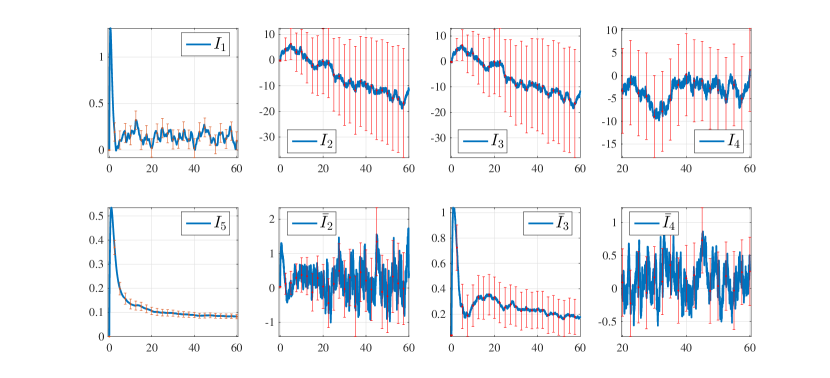
(a)

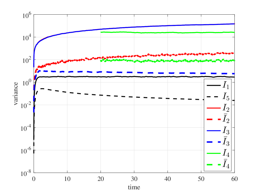
(b)

Figure 1: (a) Estimators with error bars for the derivative with respect to $\nu$ of the stochastic logistic model (22). (b) Variance of the estimators for the derivative with respect to $\nu$ of the stochastic logistic model (22) as function of time. $I_{1},I_{2},I_{3}$ and $I_{4}$: solid lines (note that the red and blue line coincide); $I_{5},\bar{I}_{2},\bar{I}_{3}$ and $\bar{I}_{4}$: dashed lines.

Here we study the logistic SDE with linear multiplicative noise which is defined through

$$dX_{t}=\nu\,X_{t}\,(1-\frac{X_{t}}{K})\,dt+\mu\,X_{t}\,dB_{t}\,,$$ (22)

where $\nu\in\mathbb{R}$ is the growth rate, $K\in\mathbb{R}^{+}$ is the capacity, $\mu\in\mathbb{R}^{+}$ the diffusion coefficient and $B_{t}$ a standard Brownian motion. This model is used as an example to illustrate the performance of estimators (6)-(14) as well as their centered variants. The parameters used for the logistic model (22) are $\nu=1,K=100,\mu=0.1,X_{0}=93$ and $T=60$. The solution of the SDE was approximated by the standard Euler-Maruyama scheme using $N=12\times 10^{3}$ points. For the finite difference estimator $\varepsilon=0.01$. The relaxation time to equilibrium is taken to be 10 and the decorrelation time $T_{d}=10$. Finally sample averages were computed over $N_{s}=1200$ sample paths.

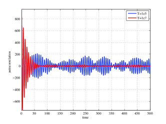
Figure 2: Autocorrelation function (ACF) for the 2nd species of the p53 model computed using a time window of width $10^{5}$ (blue line) and $10^{7}$ (red line). This is a typical example where the decorrelation length is difficult to be estimated due to the spurious oscillations.

In Figure 1(a) the sensitivity of (22) with respect to $\nu$ is presented as a function of time. Notice that although the estimators $I_{2}$ and $I_{3}$ seem to give rise the same results this is not true. The reason the estimators are so close is due to the magnitude of the noise of the score process $W$, see Appendix A, which masks the influence of the observable $f$.

In Figure 1(b) the variance of all estimators is presented. The coupling in the CFD estimator $I_{1}$ was carried out using common random numbers, see [10]. Notice that the variance of centered estimators is much smaller than that of the original LR. For the rest of the paper we will work only with the centered estimators. In accordance to the indicative analysis in (21), the proposed estimator $\bar{I}_{3}$ has constant variance in time and has the smallest variance of all the other LR estimators except the CFD estimators $I_{1}$ and $I_{5}$; the latter though become impractical in systems with a large number $N_{p}$ of parameters due to the large number of partial derivatives that need to be calculated; see also the discussion in the EGFR example below. However, note that the variance of $I_{5}$ decays for $T\gg 1$; we return to this point in the last Section of the paper. Finally, observe that the variance of $\bar{I}_{2}$ increases linearly in time as has been long-known [5].

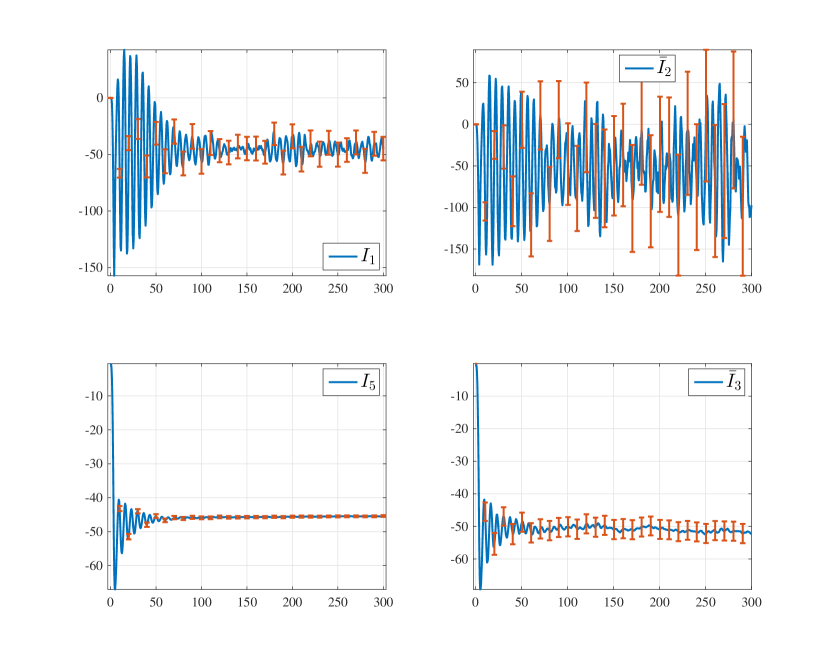
(a)

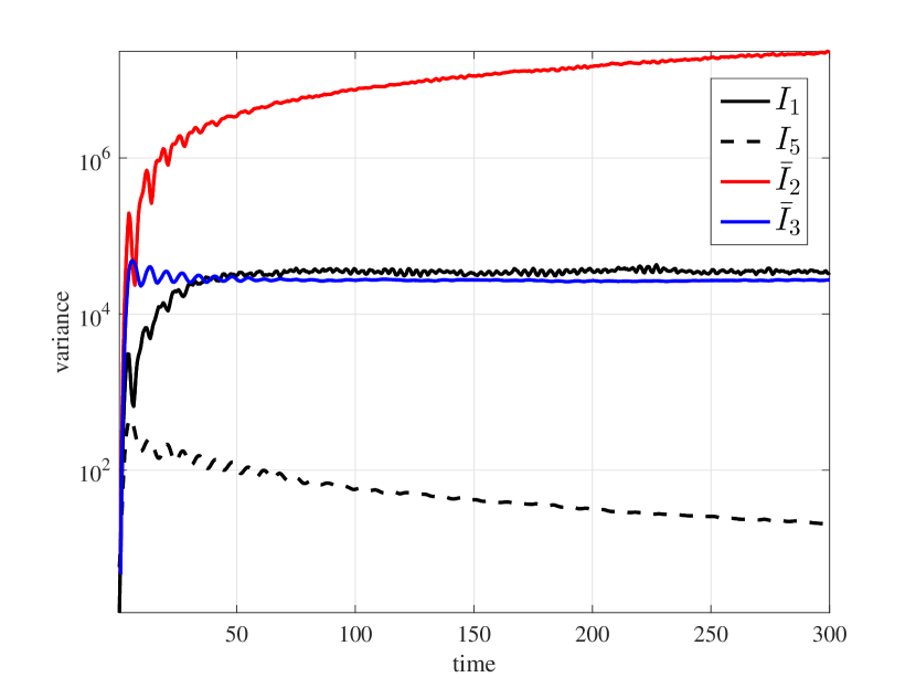
(b)

Figure 3: (a) Sensitivity index for the 2nd species with respect to the 3rd parameter of the p53 model using estimators $I_{1},\bar{I}_{2}$, $\bar{I}_{3}$ and $I_{5}$. (b) Variance of the estimators for the sensitivity index for the 2nd species with respect to the 3rd parameter of the p53 model.

3.2 Biological reaction networks

p53 reaction network: Here we compare the sensitivity estimators presented earlier in the context of a simplified p53 model [9]. The reaction network consists of 3 species, 5 reactions and 7 parameters. Detailed information of the reactions and the propensity functions, as well as the nominal values for the reaction constants, can be found in Appendix B. The parameters used here are: final time $T=50$ and for the finite difference scheme $\varepsilon=0.01$ in (6). Sample averages were computed over $N_{s}=10^{3}$ and $N_{s}=10^{4}$ sample paths for the finite difference and the log-likelihood methods, respectively. Once again the variance of $I_{1}$ and $\bar{I}_{3}$ remain constant, see Figure 3(b), and have the same (lower) variance. We return to the comparison of these two estimators in the EGFR network considered below.

In Figure 2 the autocorrelation function (ACF) of the second species is presented. The ACF is computed using a single run with a large time window. Notice that in this example an extremely large time window is needed in order to accurately compute the ACF. Furthermore the decorrelation time should be chosen at least as large as $T_{d}=200$. Here, the decorrelation time is overestimated in order to be sure that the samples are uncorrelated and was chosen to be three times $70$, where $70$ is roughly the point where the autocorrelation function approaches zero. These observations lead to the following conclusions for the use of estimator $\bar{I}_{4}$: (a) the parameter of the estimator, i.e., the decorrelation length $T_{d}$, is a sensitive quantity that needs effort and monitoring by the user to be computed; (b) the estimator becomes inefficient due to the large $T_{d}$. Thus, $\bar{I}_{4}$ is excluded from the study of the p53 model. On the other hand, the implementation of estimator $\bar{I}_{3}$ needs no monitoring by the user, hence referred to as unsupervised. In this case, due to the different (averaged) observable (2) used in (14) and the oscillations in the solution, the sensitivity index computed using $\bar{I}_{3}$ is different than using $I_{1}$ and $\bar{I}_{2}$, see Figure 3(a). However at steady states they are expected to converge to the same value due to ergodicity (5).

Note that the high variance of the LR estimator $\bar{I}_{2}$ in Figure 3(a) (growing linearly in $T$, [5]) overwhelms the estimator which does not converge to the sensitivity index and thus does not provide a conclusive result. Finally, as in the SDE example in Figure 1(b), the variance of $I_{5}$ decays for $T\gg 1$ yielding a very efficient estimator for this case; we discuss this point further in the last Section.

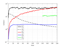
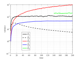
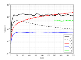
Figure 4: Variance of the estimators for the sensitivity index for the (left) 15th species with respect to the 50th parameter (middle) 18th species with respect to the 49th parameter (right) 23rd species with respect to the 47th parameter of the EGFR model as a function of time. Notice that estimator $\bar{I}_{3}$ has eventually lower variance than $I_{1}$.

EGFR reaction network: The EGFR model is a well-studied reaction network describing signaling phenomena of (mammalian) cells [19]. Here we study the reaction network developed by Kholodenko et al.  [16] which consists of 23 species, 47 reactions and a total of 50 parameters. Detailed information for the model and the nominal values for the parameters used can be found in Appendix B. The parameter used for the finite difference scheme (6) is $\varepsilon=0.01$. Sample averages were computed over $N_{s}=10^{4}$ sample paths for all estimators. The decorrelation time was chose as $T_{d}=40$ and is roughly the same for all the species.

In Figure 4 the variance of all estimators for the 15th, 18th and 23rd species with respect to the 50th, 49th and 47th parameter is presented as function of time at the transient regime up to final time $T=200$. The variance of $I_{5}$ is not always smaller than that of $\bar{I}_{3}$. However, even when the variance of $I_{5}$ is bigger, see the Figure 4 (right), it is still comparable with that of $\bar{I}_{3}$. As in previous examples, the variance of $I_{5}$ decays for $T\gg 1$; we return to this point in the last Section. After $t=30$ the system has reached steady state. In Figure 5 the sensitivity of various pairs of species and parameters is presented for all estimators at the same terminal time $T=100$. Notice that the confidence intervals of $\bar{I}_{3}$ are comparable, or even smaller, than the confidence intervals of $I_{5}$. Finally, the computational cost of $I_{1}$ and $I_{5}$ rises significantly since they need separate runs for the sensitivity of each parameter through partial derivatives calculations, for example here we have $N_{p}=50$ parameters, but also much larger systems exist in the literature; we refer to [3] for further details on sensitivity screening strategies based on (17) for systems with a large number of parameters. On the other hand $\bar{I}_{3}$ is gradient-free since it needs only one run to compute the sensitivities with respect to all parameters.

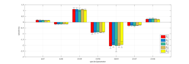
Figure 5: Sensitivity indices at equilibrium for the EGFR model for various pairs of species/parameter.

4 Discussion

Our discussion and examples make clear that the estimator $\bar{I}_{3}$ is an excellent choice as a sensitivity index for steady states, but is not appropriate for finite-time windows, unless the observable is a time average (2). However, for finite time windows the standard LR $I_{2}$ and its centered LR variant $\bar{I}_{2}$ are applicable and have bounded variance. The estimator $I_{4}$ needs explicit knowledge of the decorrelation time, $T_{d}$. In many cases this estimation is problematic, see the p53 example, and thus the use of $I_{4}$ is not recommended.

As a consequence, a reliable method combines the two LR methods, using first the standard LR estimator $\bar{I}_{2}$ and switching to the centered ergodic LR $\bar{I}_{3}$ for long times and steady state sensitivity analysis. From a practical perspective, monitoring the relaxation time of the easy to implement and low variance $\bar{I}_{3}$ suggests when to switch between $\bar{I}_{2}$ and $\bar{I}_{3}$, see for instance Fig. 1a and 2a; however this latter gluing step between finite-times and steady states may have to be supervised by the user. For example, in the p53 network, one can observe by monitoring the convergence of $\bar{I}_{3}$ that the system is equilibrated at approximately $T=100$, see Figure 3(a). Then, one can use $\bar{I}_{2}$ in the time interval $[0,T]$ and $\bar{I}_{3}$ for the computation of the sensitivity at equilibrium.

Now we turn our attention to the comparison of the ergodic estimators $\bar{I}_{3}$ and $I_{5}$. Based on the simulations presented in Figures 1b, 3b and 4, we can infer that the variance of $I_{5}$ should go to zero as $T\rightarrow\infty$, which is also expected to be mathematically correct due to ergodicity, (5). Therefore it may be plausible to argue that $I_{5}$ should be the best choice for equilibrium computations: run a single simulation for $T\gg 1$ and then estimate the sensitivity using the ergodic average $I_{5}$. However this approach may not be as efficient for high dimensional systems such as kinetic Monte Carlo, complex reaction networks or Langevin dynamics, where long time simulations are expensive or their parallelization is non-trivial. On the other hand, we can trivially parallelize the procedure, by choosing a large final time–but only big enough to ensure that the system is equilibrated–and then estimate the sensitivity using many independent simulations that can be run in parallel. In other words, for complex, high dimensional models, it may be computationally more efficient to control the variance by increasing the number $M$ of independent runs in (1) than increasing the final time $T$. It is also worth mentioning that Coupling Finite Difference (CFD) estimators such as $I_{1}$ or $I_{5}$ are biased due to the finite differencing. Furthermore, although the implementation of the CFD estimators is trivial in SDEs and fairly easy the case of biological networks, this is not true for spatial stochastic systems, as shown in [2]. Overall, we can characterize LR methods as non-intrusive in the sense that they do not require modifications to existing simulation algorithms since the are simple to implement as a standard observable; on the other hand, CFD methods are intrusive, demanding modifications to the employed stochastic simulation algorithms. In view of these observations, and taking into account the fact that the LR estimators are $2N_{p}$ times faster ($N_{p}$ is the number of model parameters) than CFD estimators as we discussed earlier in beginning of Section 3, the use of the efficient LR estimators such as $\bar{I}_{3}$ and COV are in general preferred over the CFD estimators such as $I_{1}$ and $I_{5}$.

Finally, we note that hybrid perspectives [27], (also referred as mixed estimators [10]), combine finite difference, LR and pathwise methods [21]. Overall, such an approach, in conjunction with the centered ergodic LR estimator $\bar{I}_{3}$ proposed here may prove to be a fruitful future direction towards further optimized sensitivity methods. Nevertheless, the centered ergodic (14) and the covariance LR (16), in tandem with the standard LR estimators provide a ready to use and easily implementable screening and sensitivity method, capable to handle in an unsupervised manner (at least for steady states) complex and high dimensional stochastic networks and dynamics.

Appendix A LR weights

In this section we provide some explicit formulas for the weight $W^{\theta}(X_{0:T})$ in various cases used in the paper, see e.g. [5, 4] for more details and formulas for more general processes.

1. Discrete time Markov chain on a countable state space. Let $X_{t}$ be a discrete-time Markov chain on a countable state space and transition probabilities $p^{\theta}(x,y)$. We assume that the set $\{(x,y)\,;p^{\theta}(x,y)>0\}$ does not depend on $\theta$ which implies that $P^{\theta}_{0:T}$ and $P^{\theta+\epsilon}_{0:T}$ are mutually absolutely continuous. With the score function $\nabla_{\theta}\log p^{\theta}(x,y)$ we have

$$W^{\theta}(X_{0:T})\,=\,\sum_{t=1}^{T}\nabla_{\theta}\log p^{\theta}(X_{t-1},X_{t})\,.$$ (23)

2. Countinuous time Markov chain on a countable state space. Let $X_{t}$ be a continuous-time Markov chain on a countable state space and jump rates $a^{\theta}(x,y)$ from $x$ to $y$ for $x\not=y$. We further set $a^{\theta}(x,x)=0$ and denote by $\lambda^{\theta}(x)=\sum_{y\not=x}a(x,y)$ the total jump rate from $x$. Here again we assume that the set $\{(x,y)\;a^{\theta}(x,y)>0\}$ is independent of $\theta$ which ensures $P^{\theta}_{0:T}$ and $P^{\theta+\epsilon}_{0:T}$ are mutually absolutely continuous and we have the formula

$$W^{\theta}(X_{0:T})\,=\,\int_{0}^{t}\nabla_{\theta}\lambda^{\theta}(X_{s})ds-\sum_{s\leq T}\nabla_{\theta}\log a^{\theta}(X_{s-},X_{s})\,.$$ (24)

The second term in (24) contains, almost surely, only finitely many terms corresponding to the jumps of the Markov chains between time $0$ and time $T$.

3. Stochastic differential equations. Consider the system of $N$ stochastic differential equations

$$dX_{t}=a^{\theta}(X_{t})dt+\sigma(X_{t})dB_{t}\,,$$ (25)

where $B$ is a $d$-dimensional Wiener process, $a^{\theta}(x)$ is an $N$ dimensional vector field depending on the parameter $\theta$, and $\sigma:=\sigma(x)$ an $N\times d$ matrix valued function. Typical examples are Langevin equations [24] and models in finance [10]. In this case the score process is given by the Ito integral [8],

$$W^{\theta}(X_{0:T})=\int_{0}^{T}\Gamma(X_{t})^{\top}dB_{t}\,,$$ (26)

where $\Gamma(x)$ satisfies $\sigma(x)\,\Gamma(x)=\nabla_{\theta}a(x)$, see [7] (Proposition 3.1), we also refer to [4] for more general processes with jumps.

4. Euler method for Stochastic differential equations. In numerical simulations instead of (25) one generally uses a numerical scheme, for example the Euler-Marayuma scheme given by

$$X_{n+1}=X_{n}+\Delta t\;a^{\theta}(X_{n})+\sqrt{\Delta t}\;\sigma(X_{n})\Delta B_{n}\,,$$ (27)

for $n=0,\ldots,N-1$ and $\Delta t=\frac{T}{N+1}$. Here the $\Delta B_{n}$ are i.i.d. standard normal random variables. The process $X_{n}$ is a discrete time Markov chain with a continuous state space and using the transition probabilities of $X_{n}$ one finds, as in (23), that

$$W^{\theta}(X_{0:T})=\sum_{n=1}^{N}\Gamma(X_{n-1})\,\sqrt{\Delta t}\,\Delta B_{n}\,,$$ (28)

which is, unsurprisingly, the time-discretization of the stochastic integral (26).

Appendix B Reaction networks

In this section we present the details, as well as the nominal values for the parameters, of the p53 and EGFR reaction networks presented in main text. First we note that in the context of reaction networks, in the corresponding continuous time jump processes considered in generality in Appendix A, the jump rates satisfy $a^{\theta}(x,y)=a^{\theta}(x)$.

p53 reaction network The reactions, propensity functions and reaction constants for the p53 reaction network are summarized in Table I and II.

Event	Reaction	Rate	Rate’s derivative
$R_{1}$	$\emptyset\rightarrow x$	$a_{1}(\mathbf{x})=b_{x}$	$\nabla_{\theta}a_{1}(\mathbf{x})=[1,0,0,0,0,0,0]^{\top}$
$R_{2}$	$x\rightarrow\emptyset$	$a_{2}(\mathbf{x})=a_{x}x+\frac{a_{k}y}{x+k}x$	$\nabla_{\theta}a_{2}(\mathbf{x})=[0,x,xy/(x+k),-a_{k}xy/(x+k)^{2},0,0,0]^{\top}$
$R_{3}$	$x\rightarrow x+y_{0}$	$a_{3}(\mathbf{x})=b_{y}x$	$\nabla_{\theta}a_{3}(\mathbf{x})=[0,0,0,0,x,0,0]^{\top}$
$R_{4}$	$y_{0}\rightarrow y$	$a_{4}(\mathbf{x})=a_{0}y_{0}$	$\nabla_{\theta}a_{4}(\mathbf{x})=[0,0,0,0,0,y_{0},0]^{\top}$
$R_{5}$	$y\rightarrow\emptyset$	$a_{5}(\mathbf{x})=a_{y}y$	$\nabla_{\theta}a_{5}(\mathbf{x})=[0,0,0,0,0,0,y]^{\top}$

Table 1: The reaction table where $x$ corresponds to p53, $y_{0}$ to Mdm2-precursor while $y$ corresponds to Mdm2. The state of the reaction model is defined as $\mathbf{x}=[y,y_{0},x]^{\top}$ while the parameter vector is defined as $\theta=[b_{x},a_{x},a_{k},k,b_{y},a_{0},a_{y}]^{\top}$.

Parameter	$b_{x}$	$a_{x}$	$a_{k}$	$k$	$b_{y}$	$a_{0}$	$a_{y}$
Value	90	0.002	1.7	0.01	1.1	0.8	0.8

Table 2: Parameter values for the p53 model.

EGFR reaction network

The propensity function for the $R_{j}$ reaction of the EGFR network is written in the form (mass action kinetics, see [15])

$$a_{j}(\mathbf{x})=k_{j}\binom{\mathbf{x}_{A_{j}}}{\alpha_{j}}\binom{\mathbf{x}_{B_{j}}}{\beta_{j}},\quad j=1,\ldots,47\textrm{ and }j\neq 7,14,29\ ,$$ (29)

for a reaction of the general form “$\alpha_{j}A_{j}+\beta_{j}B_{j}\xrightarrow{k_{j}}\ldots$”, where $A_{j}$ and $B_{j}$ are the reactant species, $\alpha_{j}$ and $\beta_{j}$ are the respective number of molecules needed for the reaction and $k_{j}$ the reaction constant. The binomial coefficient is defined by $\binom{n}{k}=\frac{n!}{k!(n-k)!}$. Here, $\mathbf{x}_{A_{j}}$ and $\mathbf{x}_{B_{j}}$ is the total number of species $A_{j}$ and $B_{j}$, respectively. Reactions $R_{7},R_{14},R_{29}$ are exceptions with their propensity functions being described by the Michaelis–Menten kinetics, see [15],

$$a_{j}(\mathbf{x})=V_{j}\mathbf{x}_{A_{j}}/\left(K_{j}+\mathbf{x}_{A_{j}}\right),\quad j=7,14,29\ ,$$ (30)

where $V_{j}$ represents the maximum rate achieved by the system at maximum (saturating) substrate concentrations while $K_{j}$ is the substrate concentration at which the reaction rate is half the maximum value. The parameter vector contains all the reaction constants,

$$\theta=[k_{1},\ldots,k_{6},k_{8},\ldots,k_{13},k_{15},\ldots,k_{28},k_{30},\ldots,k_{47},V_{7},K_{7},V_{14},K_{14},V_{29},K_{29}]^{\top}\ ,$$ (31)

with $K=50$. In this study the values of the reaction constants are the same as in [16].

References

- [1] D. F. Anderson. An efficient finite difference method for parameter sensitivities of continuous-time markov chains. SIAM J. Numerical Analysis, 50(5):2237–2258, 2012.
- [2] G. Arampatzis and M. Katsoulakis. Goal-oriented sensitivity analysis for lattice kinetic monte carlo simulations. J. Chem. Phys., 140(12):124108, 2014.
- [3] G. Arampatzis, M. A. Katsoulakis, and Y. Pantazis. Accelerated sensitivity analysis in high-dimensional stochastic reaction networks. PLoS ONE, 2015.
- [4] G. Arampatzis, M. A. Katsoulakis, and L. Rey-Bellet. Linear response, score functional and information-based sensitivity screening for stochastic dynamics. In preparation, 2015.
- [5] S. Asmussen and P. Glynn. Stochastic simulation: algorithms and analysis. Stochastic modelling and applied probability. Springer, New York, 2007.
- [6] P. Dupuis, M. A. Katsoulakis, Y. Pantazis, and P. Plechac. Path-space information bounds for uncertainty quantification and sensitivity analysis of stochastic dynamics. SIAM/ASA J. of Uncertainty Quantification, to appear, 2016.
- [7] E. Fournie, J. M. Lasry, J. Lebuchoux, P.-L. Lions, and N. Touzi. Applications of Malliavin calculus to Monte Carlo methods in finance. Finance and Stochastics, 3(4):391–412, 1999.
- [8] C. Gardiner. Handbook of Stochastic Methods: for Physics, Chemistry and the Natural Sciences. Springer, 4th edition, 2009.
- [9] N. Geva-Zatorsky, N. Rosenfeld, S. Itzkovitz, R. Milo, A. Sigal, E. Dekel, T. Yarnitzky, Y. Liron, P. Polak, G. Lahav, and U. Alon. Oscillations and variability in the p53 system. Molecular Systems Biology, 2:0033, 2006.
- [10] P. Glasserman. Monte Carlo methods in financial engineering. Springer, 2004.
- [11] P. Glynn. Likelihood ratio gradient estimation for stochastic systems. Communications of the ACM, 33(10):75–84, 1990.
- [12] P. W. Glynn. Likelilood ratio gradient estimation: An overview. In Proceedings of the 19th Conference on Winter Simulation, WSC ’87, pages 366–375, New York, NY, USA, 1987. ACM.
- [13] M. Hairer and A. J. Majda. A simple framework to justify linear response theory. Nonlinearity, 23(4):909–922, 2010.
- [14] A. Hashemi, M. Nunez, P. Plechac, and D. G. Vlachos. Stochastic Averaging and Sensitivity Analysis for Two Scale Reaction Networks. ArXiv e-prints, Sept. 2015.
- [15] J. D. III. Dynamic Systems Biology Modeling and Simulation. Elsevier, 2013.
- [16] B. N. Kholodenko, O. V. Demin, G. Moehren, and J. B. Hoek. Quantification of short term signaling by the epidermal growth factor receptor. Journal of Biological Chemistry, 274(42):30169–30181, 1999.
- [17] T. Liggett. Interacting particle systems. Springer - Berlin, 1985.
- [18] S. Meyn and R. Tweedie. Markov Chains and Stochastic Stability. Springer-Verlag, 1993.
- [19] N. Moghal and P. Sternberg. Multiple positive and negative regulators of signaling by the egf receptor. Curr. Opin. Cell. Biol., 11:190–196, 1999.
- [20] Y. Pantazis and M. Katsoulakis. A relative entropy rate method for path space sensitivity analysis of stationary complex stochastic dynamics. J. Chem. Phys., 138(5):054115, 2013.
- [21] P. Sheppard, M., and M. Khammash. A pathwise derivative approach to the computation of parameter sensitivities in discrete stochastic chemical systems. J. Chem. Phys., 136(3):034115, 2012.
- [22] P. W. Sheppard, M. Rathinam, and M. Khammash. SPSens: A software package for stochastic parameter sensitivity analysis of biochemical reaction networks. Bioinformatics, 29(1):140–142, 2013.
- [23] R. Srivastava, D. F. Anderson, and J. B. Rawlings. Comparison of finite difference based methods to obtain sensitivities of stochastic chemical kinetic models. J. Chem. Phys., 138(7):074110, 2013.
- [24] M. E. Tuckerman. Statistical Mechanics: Theory and Molecular Simulation. Oxford University Press, 2010.
- [25] P. B. Warren and R. J. Allen. Steady-state parameter sensitivity in stochastic modeling via trajectory reweighting. The Journal of Chemical Physics, 136(10):104106, 2012.
- [26] L. Wasserman. All of Statistics: A Concise Course in Statistical Inference. Springer, 2004.
- [27] E. S. Wolf and D. F. Anderson. Hybrid pathwise sensitivity methods for discrete stochastic models of chemical reaction systems. The Journal of Chemical Physics, 142(3):034103, 2015.