Exploring free-form smearing for bottomonium and B meson spectroscopy

Abstract:

Free-form smearing was designed as a way to implement source operators of any desired shape. A variation of the method is introduced that reduces the computational cost by reducing the number of link multiplications to its absolute minimum. Practical utility is demonstrated through calculations of bottomonium and B meson masses.

1 Motivation

To study a particular hadronic state, it would be ideal to have an operator that couples only to that state. An operator with the correct angular momentum quantum numbers is necessary but not sufficient. The spatial structure of the operator (i.e. its “shape”) helps to distinguish states with different principal quantum numbers.

Free-form smearing was designed as a way to implement source operators of any desired shape [1] and a variation of the method has been introduced that reduces the computational cost by reducing the number of link multiplications to its absolute minimum [2].

An explicit implementation of the new method is provided here, and the practical utility of the algorithm is demonstrated through calculations of bottomonium and $B_{c}$, $B_{s}$ and $B$ meson masses.

2 Free-form smearing

Though free-form smearing can be applied to a quark propagator in any context, consider for definiteness a meson operator defined at a lattice site $x$. Let $\chi(x)$ represent the antiquark field and let $\tilde{\tilde{\psi}}(x)$ represent the free-form smeared quark field. The meson operator is then

$$\chi(x)\tilde{\tilde{\psi}}(x)=\chi(x)\sum_{y}\Omega(x-y)\frac{\tilde{\psi}_{x}(y)}{\left<\left|\left|\tilde{\psi}_{x}(y)\right|\right|\right>}$$ (1)

where $\Omega(x-y)$ is chosen by the user to define the desired shape and quantum numbers of the operator. The denominator is the ensemble average of a color+Dirac trace

$$\left<\left|\left|\tilde{\psi}_{x}(y)\right|\right|\right>=\sqrt{{\rm Tr}\left(\tilde{\psi}_{x}^{\dagger}(y)\tilde{\psi}_{x}(y)\right)}$$ (2)

and its purpose is to divide out spatial variations in the quark field $\tilde{\psi}_{x}(y)$ so the interpretation of $\Omega(x-y)$ is as transparent as possible.

The original implementation of free-form smearing defined $\tilde{\psi}$ through standard Gaussian smearing, but a more efficient definition is the minimal-path definition, where no paths are duplicated in the calculation:

$$\tilde{\psi}_{x}(y)=\sum_{\rm shortest~{}paths}U(x\to y)\psi(y)$$ (3)

The link variables in $U(x\to y)$ can be thin or thick; our examples use stout links [3].

3 The minimal-path algorithm to compute $\tilde{\psi}_{x}(y)$

The algorithm to compute the minimal paths of links is presented as pseudocode in Alg. 1. Free-form smearing can then be implemented as described in Sec. 2. Whereas the Gaussian version of free-form smearing requires $O(L^{4})$ link multiplications, the minimal-path method uses only $3L^{3}$ link multiplications, which is exactly the number of spatial links on a given time slice and is therefore the minimal number of link multiplications.

Algorithm 1 An implementation of the minimal-path algorithm for free-form smearing.

blue

sitevisited = false $\triangleright$ blackInitialize all sites and links as having not been visited. blue

linkvisited = false blue

$\tilde{\psi}=0$ $\triangleright$ blackInitialize the field to unity at the origin and zero everywhere else. blue

$\tilde{\psi}(x)=1$ blue

sitevisited$(x)$ = true $\triangleright$ blackMark the origin, $x$, as having been visited. blue

$y_{\rm frontier}(1)=x$ $\triangleright$ blackMark the origin, $x$, as on the frontier. blue

$n=1$ $\triangleright$ blackInitially there is only one point on the frontier. blue

while $n>0$ do $\triangleright$ blackLoop until all sites are visited, i.e. the frontier contains no points $(n=0)$. blue

     $n_{\rm new}=0$ $\triangleright$ blackInitialize the number of points on the new frontier to zero. blue

     for $i=1,n$ do $\triangleright$ blackVisit all of the points on the frontier. blue

         $y=y_{\rm frontier}(i)$ blue

         for $\mu=1,3$ do blue

              $\triangleright$ blackFORWARD DIRECTION: blue

              if linkvisited$(\mu,y)$ = false then $\triangleright$ blackIf the link $U_{\mu}(y)$ has not been visited. blue

                  $\tilde{\psi}(y+\mu)=\tilde{\psi}(y+\mu)+U^{\dagger}_{\mu}(y)\tilde{\psi}(y)$ $\triangleright$ blackUse $U_{\mu}(y)$ to update the new frontier. blue

                  linkvisited$(\mu,y)$ = true $\triangleright$ blackMark this link as visited. blue

                  if sitevisited$(y+\mu)$ = false then $\triangleright$ blackIf this site has not been visited before. blue

                       sitevisited$(y+\mu)$ = true $\triangleright$ blackMark this site as visited. blue

                       $n_{\rm new}=n_{\rm new}+1$ $\triangleright$ blackThe new frontier is larger. blue

                       $y_{\rm newfrontier}(n_{\rm new})=y+\mu$ $\triangleright$ blackAdd this site to the new frontier. blue

                  end ifblue

              end ifblue

              $\triangleright$ blackBACKWARD DIRECTION: blue

              if linkvisited$(\mu,y)$ = false then $\triangleright$ blackIf the link $U_{\mu}(y-\mu)$ has not been visited. blue

                  $\tilde{\psi}(y-\mu)=\tilde{\psi}(y-\mu)+U_{\mu}(y-\mu)\tilde{\psi}(y)$ $\triangleright$ blackUse $U_{\mu}(y-\mu)$ to update new frontier. blue

                  linkvisited$(\mu,y)$ = true $\triangleright$ blackMark this link as visited. blue

                  if sitevisited$(y-\mu)$ = false then $\triangleright$ blackIf this site has not been visited before. blue

                       sitevisited$(y-\mu)$ = true $\triangleright$ blackMark this site as visited. blue

                       $n_{\rm new}=n_{\rm new}+1$ $\triangleright$ blackThe new frontier is larger. blue

                       $y_{\rm newfrontier}(n_{\rm new})=y-\mu$ $\triangleright$ blackAdd this site to the new frontier. blue

                  end ifblue

              end ifblue

         end forblue

     end forblue

     $n=n_{\rm new}$ $\triangleright$ blackSites in the new frontier become sites in the old frontier. blue

     $y_{\rm frontier}=y_{\rm newfrontier}$ blue

end while

4 Sample smearing shapes

To smear a bottom quark for use in bottomonium or a bottom-flavored meson, we choose $\Omega(x-y)$ to have a Coulomb wave function shape (familiar from the quantum mechanics of hydrogen) as well as the requisite $J^{P}$ quantum numbers. All of the $\Omega(x-y)$ functions from S wave to G wave are listed in [2] so only the first few are displayed here, in Table 1.

Table 1: The $\Omega(x-y)$ functions of Eq. (1) that represent Coulomb wave function shapes for S-wave and P-wave mesons can be expressed as $\Omega(x-y)=e^{-r/a_{0}}f(x-y)$. A few of the $f(x-y)$ are tabulated here.

${}^{2S+1}L_{J}$	0th radial	1st radial	2nd radial
${}^{1}S_{0}$	1	$(r-b)$	$(r-c)(r-b)$
${}^{3}S_{1}$	$\sigma_{i}$	$(r-b)\sigma_{i}$	$(r-c)(r-b)\sigma_{i}$
${}^{1}P_{1}$	$\sin\left(\frac{2\pi}{L}(x_{i}-y_{i})\right)$	$(r-b)\sin\left(\frac{2\pi}{L}(x_{i}-y_{i})\right)$
${}^{3}P_{0}$	$\sum_{i=1}^{3}\sigma_{i}\sin\left(\frac{2\pi}{L}(x_{i}-y_{i})\right)$	$(r-b)\sum_{i=1}^{3}\sigma_{i}\sin\left(\frac{2\pi}{L}(x_{i}-y_{i})\right)$

The radius and nodal parameters $(a_{0},b,c)$ are tuned for each hadron to optimize the signal, and in all of the studies reported here they satisfy $0.5\leq a_{0}\leq 7.0$ and $2.1<b\leq 6.2$ and $c=6.0$ in lattice units. These parameters are determined quite precisely for each meson, and the ranges listed here are only to provide a notion of typical numerical values. The argument $r$ of $\Omega(r)$ is defined by

$$r=\sqrt{(x_{1}-y_{1})_{\rm min}^{2}+(x_{2}-y_{2})_{\rm min}^{2}+(x_{3}-y_{3})_{\rm min}^{2}}.$$ (4)

5 Simulation details

The spectrum calculations presented here use an ensemble of 198 configurations produced by the PACS-CS collaboration [4]. Bottom quark propagators are computed with $O(v^{4})$ tadpole-improved lattice NRQCD. All other quark propagators are clover-improved Wilson fermions computed using the sap_gcr solver from DD-HMC [5]. Parameters for the charm quark, following the Fermilab interpretation, are from [6].

Three methods were combined to increase statistical precision: (1) a random U(1) wall source was used, with support from $4^{3}$ evenly spaced lattice sites, (2) correlators were averaged over sources on different time slices (every time step for bottomonium or every second time step for bottom mesons), (3) NRQCD propagators were calculated forward and backward in time.

6 Results

To verify orthogonality based on operator shape, Fig. 1 shows effective mass plots for the ${}^{3}D_{2}$ bottomonium operators for the zero’th and first radial excitations. Notice that the $n$=2 result shows no contamination from the lighter $n$=1 meson. This success is particularly satisfying because no signal for $2^{3}D_{2}$ bottomonium has been reported in the lattice QCD literature before this work.

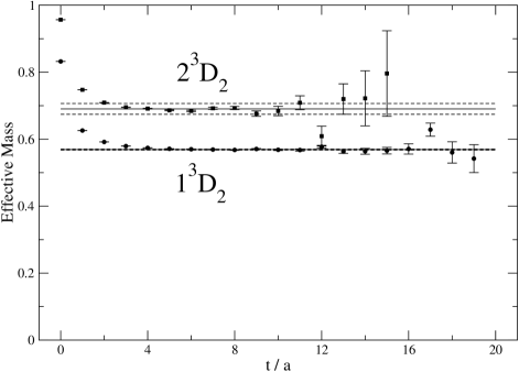
Figure 1: Effective mass plots demonstrating that the $n=2$ operator is orthogonal to the $n=1$ operator for ${}^{3}D_{2}$ bottomonium.

To determine the complete spectrum, several operators were used for each $J^{PC}$ channel and a simultaneous fit was performed. Summary plots are shown in Figs. 2, 3, 4, and 5 and include experimental data [7, 8, 9, 10, 11] where available. For further details, please consult [2].

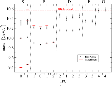
Figure 2: The bottomonium spectrum obtained using minimal-path free-form smearing.

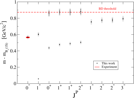
Figure 3: The $B_{c}$ meson spectrum obtained using minimal-path free-form smearing.

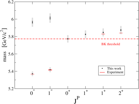
Figure 4: The $B_{s}$ meson spectrum obtained using minimal-path free-form smearing.

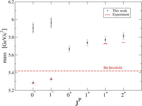
Figure 5: The $B$ meson spectrum obtained using minimal-path free-form smearing.

References

• [1] G.Β M.Β von Hippel, B.Β JΓ€ger, T.Β D.Β Rae and H.Β Wittig, JHEP 1309, 014 (2013).
• [2] M.Β Wurtz, R.Β Lewis and R.Β M.Β Woloshyn, Phys.Β Rev.Β D 92, 054504 (2015).
• [3] C.Β Morningstar and M.Β J.Β Peardon, Phys.Β Rev.Β D 69, 054501 (2004).
• [4] S.Β Aoki et al. [PACS-CS Collaboration], Phys.Β Rev.Β D 79, 034503 (2009).
• [5] M.Β LΓΌscher, Comput.Β Phys.Β Commun.Β  165, 199 (2005).
• [6] C.Β B.Β Lang, L.Β Leskovec, D.Β Mohler, S.Β Prelovsek and R.Β M.Β Woloshyn, Phys.Β Rev.Β D 90, 034510 (2014).
• [7] K.Β A.Β Olive et al. [Particle Data Group Collaboration], Chin.Β Phys.Β C 38, 090001 (2014).
• [8] T.Β A.Β Aaltonen et al. [CDF Collaboration], Phys.Β Rev.Β D 90, 012013 (2014).
• [9] G.Β Aad et al. [ATLAS Collaboration], Phys.Β Rev.Β Lett.Β  113, 212004 (2014).
• [10] R.Β Aaij et al. [LHCb Collaboration], JHEP 1410, 88 (2014).
• [11] R.Β Aaij et al. [LHCb Collaboration], JHEP 1504, 024 (2015).