Brownian dynamics simulations of an idealized chemical reaction network under spatial confinement and crowding conditions

Abstract

234

I Introduction

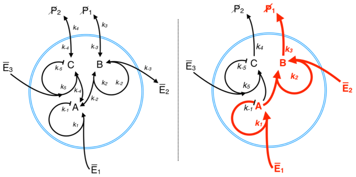
Figure 1: Schematic view of the Willamowski-Rossler chemical network. (Left) the full version. (Right) the minimal version analyzed in this study, obtained by setting $k_{-2}=k_{-3}=k_{-4}=0$. In red we highlight the Lotka-Volterra component of the network. The rate equations for both versions exhibit three different dynamical regimes: fixed point, limit cycle and chaotic Willamowski and Rossler (1980); Stucki and Urbanczik (2005).

Biochemical networks in vivo are typically open to the exchange of energy and matter with the surrounding environmentQian (2006, 2007); Ritort (2008); Stano and Luisi (2013). They often contain autocatalytic steps McNaught and Wilkinson (1997); Lee et al. (1997); Dadon et al. (2008); Virgo and Ikegami (2013); Hordijk et al. (2010) and their dynamics tends to be strongly influenced by thermal and intrinsic noise Johnson (1987); Gillespie (1977), macromolecular crowding and spatial confinement Minton (1981, 1998, 2001); Richter et al. (2007, 2008). In this study we present a simple computational model of a generic biochemical network in vivo and we investigate how its dynamics is affected by spatial confinement and particle crowding. Minton (1981, 1998, 2001); Richter et al. (2007, 2008). Our model is based on the Willamowski-Rossler (WR) chemical network Willamowski and Rossler (1980). The WR network (see Figure 1(a)) is a non-linear chemical system based on zeroth, first and second order chemical reactions. It contains three autocatalytic steps involving species $A$,$B$ and $C$ and it is thermodynamically open Qian (2006, 2007); Ritort (2008); Stano and Luisi (2013). Its rate equations display a rich and complicated dynamics comprising fixed point, limit cycle and chaotic attractors. The WR network has been previously studied via deterministic and non-spatial stochastic simulation methods Aguda and Clarke (1988); Guemez and Matias (1993); Geysermans and Nicolis (1993); Goryachev and Kapral (1996); Chavez and Kapral (2002); Stucki and Urbanczik (2005) but never as a stochastic reaction–diffusion system where crowding and spatial confinement are explicitly taken into account.

In detail, we investigate the effects of spatial confinement and crowding on a minimal version of the WR network (MWR) (see Figure 1(b) and Ref. Stucki and Urbanczik, 2005) using hard-sphere Ando and Skolnick (2010); Ando and Jeffrey (2011) Brownian dynamics simulations integrating chemical reactivity Morelli and ten Wolde (2008); Frazier and Alber (2012). We fix the population numbers for species $E_{1}$, $E_{2}$, $E_{3}$, $P_{1}$ and $P_{2}$ (consequently the rates $k_{1}$, $k_{3}$ and $k_{5}$ become pseudo-first order) so that the MWR network is thermodynamically open. The following chemical reactions describe the MWR system used in our simulations Stucki and Urbanczik (2005) (see also Figure 1(b)).

The main assumption in the MWR system Willamowski and Rossler (1980); Stucki and Urbanczik (2005) is that three of the backward reaction rate constants shown in Figure 1(a), namely $k_{-2}$, $k_{-3}$ and $k_{-4}$, are much smaller than their forward counterparts and, hence, can be neglected (See Figure 1(b)). The MWR system is composed by two main subsystems: a Lotka-Volterra oscillator Lotka (1910, 1920); Volterra (1926) involving species $A$ and $B$ and a chemical switch Aguda and Clarke (1988) that couples the Lotka-Volterra component to species $C$. Similarly to the ‘full’ WR network, the MWR rate equations derived from the set of chemical reactions $(1a)-(1e)$ display a diverse dynamical behavior comprising fixed point, limit cycle and chaotic attractors Willamowski and Rossler (1980); Stucki and Urbanczik (2005). We quantify the effects of confinement and crowding on the population dynamics, flux of information and spatial organization within the MWR network. Our approach and analysis can be naturally extended to more complicated chemical networks and can be potentially relevant to a number of open problems in biochemistry such as the synthesis of primitive cellular units (protocells) and the definition of their role in the chemical origin of life, the characterization of vesicle-mediated drug delivery processes and, more generally, the study of biochemical networks in vivo Rasmussen et al. (2008); Stano and Luisi (2013); Luisi et al. (2006); Szathmary (2005). We make the case for a more widespread development and use of spatial stochastic simulation methods for biochemical networks in vivo that explicitly take into account confinement and macromolecular crowding Beck et al. (2011); Gillespie et al. (2013); Andersen (2005); Minton (1981).

II Methods

All three autocatalytic species $A$, $B$ and $C$ are spatially confined within a spherical container, $E_{1}$ and $E_{3}$ catalyze the synthesis of $A$, and $C$, respectively, whereas $E_{2}$ catalyzes the degradation of $C$. $P_{1}$ and $P_{2}$ are the products of reactions $(1d)$ and $(1c)$, respectively, and they get instantaneously eliminated from the reaction pool, i.e., their constant population number is zero. The constant population numbers of $E_{1}$, $E_{2}$ and $E_{3}$ and the instantaneous elimination of $P_{1}$ and $P_{2}$ lead to a biochemical network composed by $A$, $B$ and $C$ which is spatially enclosed and thermodynamically open, i.e., it exchanges matter and energy with the surrounding environment by means of three sources ($E_{1}$, $E_{2}$ and $E_{3}$) and two sinks ($P_{1}$ and $P_{2}$). The constant values of $E_{1}$, $E_{2}$, $E_{3}$ are incorporated into the pseudo-first order rates $k_{1}$, $k_{3}$, $k_{5}$, respectively (see Figure 1).

The different chemical species in the MWR system are modeled as reactive, Brownian hard spheres confined in a spherical container. The details of the Brownian integrator used in our simulations can be found in Refs. Morelli and ten Wolde, 2008; Frazier and Alber, 2012. The radius of the hard spheres for species $A$, $B$, and $C$ is $0.01$ $\mu m$ and the diffusion coefficient is $D=0.01$ $\mu m^{2}s^{-1}$. In all our simulations the time step is fixed at $\Delta t=0.01$ $s$.

To study the effects of crowding and confinement we run two separate sets of reactive Brownian dynamics simulations. In the first set we consider six different spherical containers with radius varying between $0.4$ and 0.65 $\mu m$. The containers are implemented as ‘hard-wall’ spherical boundary conditions. For each of the six spherical containers we run a total of $30$ independent simulations, each of total time $t_{tot}=1000$ $s$. Three sets of values for the reaction rate constants (kset1, kset2, kset3) are used for each one of the six different spherical containers. They correspond to three distinct dynamical behaviors in the deterministic implementation of the MWR model: fixed point, limit cycle and chaotic dynamics, respectively. The first set (kset1, fixed point attractor) is $k_{1}=30.0$, $k_{-1}=0.25$, $k_{2}=1.0$, $k_{3}=10.0$, $k_{4}=0.4$, $k_{5}=16.5$, $k_{-5}=0.5$. To generate the second set (kset2 - limit cycle attractor) we simply consider the first set of parameters and change the value of $k_{4}$ to $0.6$. In the third set (kset3 - chaotic attractor) we set $k_{4}=0.6$, $k_{5}=18.5$ and $k^{-5}=0.4$. In other words, kset2 is generated from kset1 by increasing the degradation of A and C (increasing the coupling between the Lotka-Volterra component and the switch) while kset3 is obtained from kset1 by increasing both the $A-C$ coupling and decreasing the ratio $k_{-5}/k_{5}$. We run $10$ independent simulations for each of the three parameter sets. The starting point for each simulation is generated randomly placing $A=B=C=100$ hard spheres within the proper spherical container. In the second set of simulations we take into account the presence of a variable number of ‘chemically inert’ crowders modeled as hard spheres of radius $r=0.01$ $\mu m$ and with diffusion coefficient $D=0.01$ $\mu m^{2}s^{-1}$. The starting point for each simulation in the second set is generated randomly placing $A=B=C=100$ hard spheres and a variable number of inert crowders in a spherical container with radius $R=0.4$ $\mu m$. We run independent simulations for five different crowder population numbers: varying between $2\times 10^{3}$ and $8\times 10^{3}$. For each of the five crowder population numbers we run a total of $30$ independent simulations ($10$ for each of the three parameters sets), each of total time $t_{tot}=1000$ $s$.

III Results and Discussion

III.1 Population dynamics

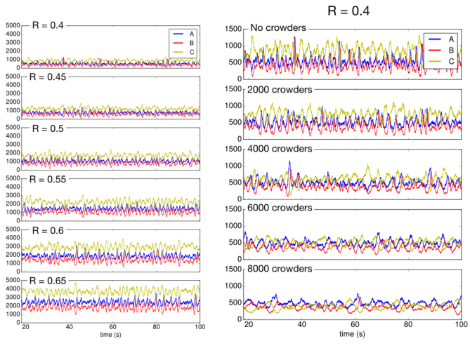
Figure 2: Population time series (partial time window) obtained each from a single trajectory of our brownian dynamics simulations of the MWR network with kset3 parameterization. Left panel: population time series for systems with varying volume (radii varying from $0.4$ to $0.65$ $\mu$m). Right panel: population time series for systems with varying number of crowders and with constant container volume (radius is $0.4$ $\mu$m).

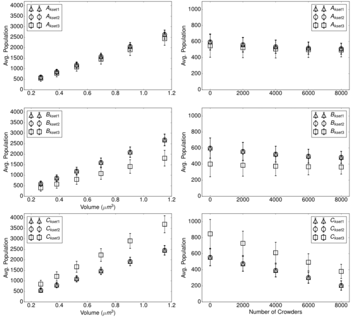
Figure 3: Average population values for species $A$ (top), $B$ (middle) and $C$ (bottom) with parameterizations kset1, kset2 and kset3. Left panel: the average populations are plotted against the volume of the spherical container, no inert crowders are present. The average population of the reactive species grows linearly with the volume of the spherical container . Right panel: the average populations are plotted against the number of inert crowders. A slight decrease in the average population is observed for larger crowders numbers.

We focus our analysis on the stationary Van Kampen (2007) portion of our Brownian simulations. In Figure 2 we show a set of representative time windows for the population numbers of species $A$, $B$ and $C$ related to simulations with variable container volume (left panel), and to simulations with constant container volume and varying number of inert crowders (right panel). All data refer to parameterization kset3 (see Section II). Time series population data generated under kset1 and kset2 are not shown as they display analogous temporal patterns. Figure 2 qualitatively shows that (1) both average population and fluctuations increase with increasing container volume for all species and (2) the presence of an increasing number of inert crowders affects the average population of species $A$, $B$ and $C$. It also appears to lower both the fluctuations in the population dynamics and the temporal interdependence between the different species. A quantitative assessment of the mean and fluctuations dependence from both the container volume and the crowders number is given in Figure 3. In the left panel we show that in the limited range of container volumes considered in our simulations, the mean population increases linearly with increasing container volume. The fluctuations calculated as the standard deviation from the mean also have a tendency to increase although the actual functional dependency is not immediately clear. The effects of the presence of inert crowders are shown in the right panel of Figure 3. All species show a decrease in their average population for increasing crowders numbers which can be intuitively related to the diminished availability of free volume within the spherical container. An additional observation on the data in Figure 3 relates to the dependence of the average population from the parameterization set. First, the population dynamics of species $A$, $B$ and $C$ does not change significantly when the parameterization set changes from kset1 to kset2. Second, the transition from parameterization kset1 and kset2 to kset3 has opposite effects on species $B$ and $C$. Third, species $A$ does not show any quantifiable dependence from the parameter set (under both volume and crowders’ number varying conditions). It is easy to connect the increase in the slope of the $C$(volume) linear fit to the increase in $C$’s net synthesis going from kset1 and kset2 to kset3. The decrease in the linear fit’s slope for species $B$ is less clear since species $B$ is not directly affected by the changes in the parameterization set and species $A$, which is directly coupled to $B$, is insensitive to those changes. The insensitivity to parameter changes in species $A$ can be qualitatively explained considering that $A$ is the connection point in the MWR network between the Lotka-Volterra component and the switch component Aguda and Clarke (1988) and therefore benefits from the ‘modulation’ given by the interaction with both species $B$ and $C$.

III.2 Information flux and statistical complexity

A possible explanation of the peculiar behavior of species $A$ and its relation with $A$’s ‘double coupling’ within the MWR network comes from the analysis of the information flux quantified by the transfer entropy defined as a particular case of the conditional mutual information Schreiber (2000); Hlavackova-Schindler et al. (2007); Vejmelka and Palus (2008):

$$\max_{\tau}I(Y(t),X(t+\tau)|X(t)),$$ (1b)

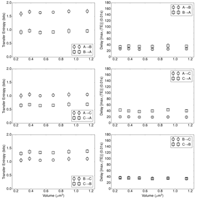
Figure 4: Left panel: transfer entropy as a function of the container volume. Right panel: characteristic time delay correspondent to the maximum value of the transfer entropy. Data refer to kset3 parameterization.

where $I(X,Y|Z)$ is the mutual information between $X$ and $Y$ given $Z$ Cover and Thomas (2006) and $\tau$ is the time delay. We employ transfer entropy to estimate both the amount and the direction of the information flux in the MWR network. The value of the delay parameter $\tau$ considered in our calculations corresponds to the maximum of the transfer entropy for a given trajectory pair. A number of interesting conclusions can be inferred from the analysis of the transfer entropy data in Figures 4 and 5. Considering first the chemical network as a whole it is worth noting that the varying container volume does not significantly affect the information flux between the different species in the network. For systems with variable number of inert crowders there is a small but noticeable systematic increase in the transfer entropy with differences between the less and the most crowded systems of the order of $0.3-0.4$ bits. A further look at the behavior of the single species shows the pivotal role of species $A$ as a common influencer of the dynamics of species $B$ and $C$. Both Figure 4 and 5 show that the amount of information transferred from species $A$ is systematically larger than the information transferred to species $A$ in both volume-varying and crowding number-varying systems. This asymmetry in the information flux (common to all three parameterization sets kset1, kset2 and kset3 - data not shown) can be linked to an increased ability of $A$ to ‘absorb’ external perturbations and therefore to its lower sensitivity to parameter change (see previous Section). The main difference in terms of information transfer between systems with and without inert crowders (see Figures 4 and 5, respectively) is in the characteristic time delay $\tau$ (see Equation 1b) at which the information transfer is maximal. While the characteristic delay $\tau$ is not affected by changes in the container volume (right panel in Figure 4), the presence of an increasing number of inert crowders in a constant volume container decreases the speed at which the information is transferred within the network (right panel in Figure 5).

In order to improve the clarity and conciseness of our manuscript, from now on we focus only on simulations performed under parameterization set kset3 as this set of parameters seems to have an additional layer of complexity with respect to kset1 and kset2 (data not shown) and carries all the significant information about our system. Information theory functionals can be also used to estimate the degree of complexity in the time evolution of the chemical network and its dependence from the container volume and from the presence of crowders. The complexity estimation quantity that we choose is an intensive statistical complexity measure which is the product of the normalized spectral entropy $\hat{S}(P_{r})$ and the intensive Jensen-Shannon divergence $\hat{Q}(P_{r},P_{e})$ Powell and Percival (1979); Rosso et al. (2007) defined respectively as:

$$\hat{S(P_{r})}=-S_{0}\sum_{r^{\prime}}^{N_{f}}P_{r^{\prime}}\log_{2}P_{r^{\prime}}$$ (1c)

with

$$P_{r}=\frac{f_{r}^{2}}{\sum_{r^{\prime}}^{N_{f}}f_{r^{\prime}}^{2}},$$ (1d)

where $f_{r}$ are the frequencies in the Fourier spectrum and $N_{f}=4000$ is the number of frequencies considered, and

$$\hat{Q}(P_{r},P_{e})=Q_{0}\Big{[}S\Big{(}\frac{P_{r}+P_{e}}{2}\Big{)}-\frac{1}{2}S(P_{e})-\frac{1}{2}S(P_{r})\Big{]},$$ (1e)

where $S(P_{e})=\log_{2}N_{f}=S_{0}^{-1}$ and $Q_{0}$ is the normalization factor for $Q$ and $P_{e}=1/N_{f}$.

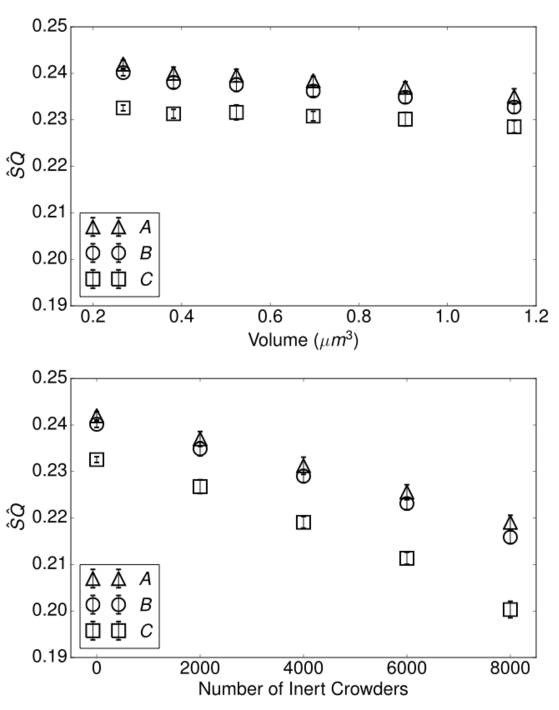
Figure 6: Statistical complexity measure as a function of the container volume (top) and number of inert crowders (bottom). Data refer to species $A$, $B$, $C$ under kset3 parameterization.

The statistical complexity $\hat{S}\hat{Q}$ is zero for both $P_{r}=\{1,0,0,\cdots,0\}$ and $P_{r}=P_{e}=1/N_{f}$, i.e., for spectral entropy $S=0$ and $S=\log_{2}N_{f}$ (fully ordered and fully stochastic systems) Rosso et al. (2007). The results for the statistical complexity $\hat{S}\hat{Q}$ are shown in Figure 6. The top panel shows that container volume variability does not significantly affect the average statistical complexity for species $A$, $B$ and $C$ (both $\hat{S}and\hat{Q}$ do not vary significantly - ${\\ }Deltaleq0.02$). Conversely, for systems with constant volume and variable crowders number the statistical complexity decreases with increasing number of crowders. In detail, the decrease is almost exclusively due to a decrease in the normalized spectral entropy from $0.62$ to $0.55$, $0.61$ to $0.54$ and $0.58$ to $0.50$, for species $A$, $B$ and $C$, respectively. The intensive Jensen-Shannon divergence remains constant at around $0.39-0.40$. As a general conclusion from our information theoretic analysis, we can state that the presence of a growing number of inert crowders drives the chemical network toward a lower degree of complexity which is possibly driven by a more efficient information transfer Figure 5) between the reactive chemical species.

III.3 Spatial statistics

The spatial organization of the chemical species in the network and its coupling with their population sizes are investigated employing a deterministic implementation of the DBSCAN clustering algorithm Ester et al. (1996), where ‘boundary’ particles are discarded as noise and with parameterization $\epsilon=0.06\mu$m and $n_{c}=4$. $\epsilon$ is the cutoff distance defining particle pairs belonging to the same cluster and therefore ‘connected’ to each other, and $n_{c}$ is the minimum number of ‘connections’ that defines a ‘core’ particle Ester et al. (1996). The presence of inert crowders strongly influences the spatial organization of the chemical species $A$, $B$ and $C$ in the MWR network.

In Figure 7 we show the average number of clusters (top) and average maximum cluster size (bottom) as a function of the number of inert clusters. On the one hand, the average number of clusters shows a weak tendency to increase for all three chemical species. On the other hand, the average maximum cluster size decreases with denser crowding conditions. Among the three reactive species the maximum cluster size in species $C$ displays both the largest values and the largest decrease rate. Figure 7 basically shows that the presence of an increasing number of crowders opposes the natural tendency of the reactive particles in our system to accumulate in well-defined regions of the available space. An interesting feature of the maximum cluster size temporal evolution is shown in Figure 8. For small numbers of crowders the maximum cluster size for species $A$ tightly mirrors the time evolution of the population of species $A$ (species $B$ and $C$ show very similar behavior - data not shown). The ‘correlation’ between population dynamics and maximum cluster dynamics weakens with increasing crowders number. Indeed, table 1 shows that the mutual information Cover and Thomas (2006) between population and maximum cluster dynamics decreases with increasing crowders numbers.

IV Conclusions

In this study we investigate the dynamical behavior of a simple chemical network under spatial confinement and crowding. We observe that the presence of inert crowders affects in a non-trivial way the population dynamics of the reactive species in the network. The detailed analysis of the population dynamics of the MWR network under different confinement and crowding conditions presented in Section III represents, from a more general perspective, an example of the level of detail, not accessible to deterministic and stochastic well-mixed models, that can be resolved when spatial confinement and crowding are explicitly taken into account. In conclusion, we try to make the case for the use of spatial stochastic simulations as an elective method to complement experiments and to improve our understanding of complex systems where dynamics is both spatially confined and compartmentalized.

Table 1: Mutual information between population size and largest cluster size for species $A$, $B$ and $C$ and for different numbers of inert crowders.

Inert Crowders	A	B	C
0	0.969	0.811	1.574
2000	0.893	0.643	1.359
4000	0.847	0.619	0.806
6000	0.611	0.583	0.735
8000	0.568	0.471	0.442

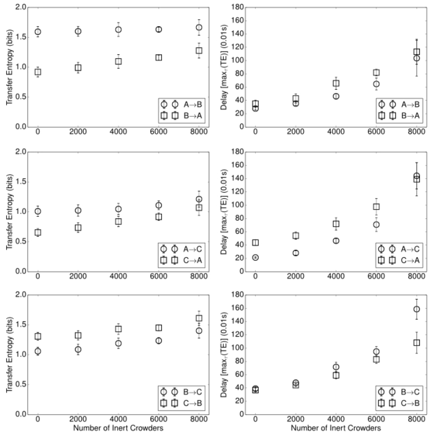
Figure 5: Left panel: transfer entropy as a function of the number of inert crowders. Right panel: characteristic time delay correspondent to the maximum value of the transfer entropy. Data refer to kset3 parameterization.

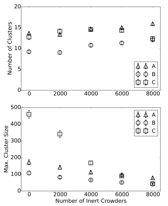
Figure 7: Average number of clusters (top) and average maximum cluster size (bottom) as a function of the number of inert clusters. Data refer to species $A$, $B$, $C$ under kset3 parameterization. The average number of clusters shows a weak tendency to increase for all three chemical species. The average maximum cluster size decreases with denser crowding conditions. The max. cluster size in species $C$ displays the largest decrease rate.

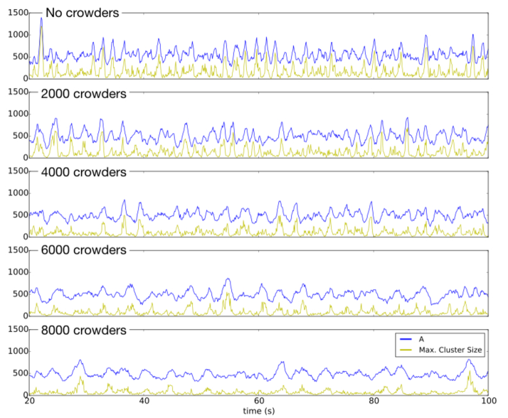
Figure 8: Time evolution for the population size (blue) and the maximum cluster size (yellow). The temporal pattern in the maximum cluster size accurately mirrors the population size. Data refer to species $A$ under kset3 parameterization. The mutual information between the two sets of temporal data decreases with increasing number of crowders (see Table 1).