Uniform Sobolev inequalities for second order non-elliptic differential operators

Abstract.

We study uniform Sobolev inequalities for the second order differential operators $P(D)$ of non-elliptic type. For $d\geq 3$ we prove that the Sobolev type estimate $\|u\|_{L^{q}(\mathbb{R}^{d})}\leq C\|P(D)u\|_{L^{p}(\mathbb{R}^{d})}$ holds with $C$ independent of the first order and the constant terms of $P(D)$ if and only if $1/p-1/q=2/d$ and $\frac{2d(d-1)}{d^{2}+2d-4}<p<\frac{2(d-1)}{d}$. We also obtain restricted weak type endpoint estimates for the critical $(p,q)=(\frac{2(d-1)}{d},\frac{2d(d-1)}{(d-2)^{2}})$, $(\frac{2d(d-1)}{d^{2}+2d-4},\frac{2(d-1)}{d-2})$. As a consequence, the result extends the class of functions for which the unique continuation for the inequality $|P(D)u|\leq|Vu|$ holds.

1. Introduction

Let $Q$ be a non-degenerate real quadratic form defined on $\mathbb{R}^{d}$, $d\geq 3$, which is given by

(1.1) $$Q(\xi)=-\xi_{1}^{2}-\cdots-\xi_{k}^{2}+\xi_{k+1}^{2}+\cdots+\xi_{d}^{2},$$

where $1\leq k\leq d$. We consider the constant coefficient second order differential operator

$$P(D)=Q(D)+\sum_{j=1}^{d}a_{j}D_{j}+b,$$

where $D=(D_{1},\cdots,D_{d})$, $D_{j}=\frac{1}{2\pi i}\frac{\partial}{\partial x_{j}}$ and $a_{1},\cdots,a_{d}$, $b$ are complex numbers. We call $P$ ‘elliptic’ if $k=d$ and ‘non-elliptic’ otherwise.

The Sobolev type estimate

(1.2) $$\|u\|_{L^{q}(\mathbb{R}^{d})}\leq C\|P(D)u\|_{L^{p}(\mathbb{R}^{d})}$$

which holds for $u\in W^{2,p}(\mathbb{R}^{d})$ has been of interest in connection to studies of partial differential equations. Here the function space $W^{2,p}(\mathbb{R}^{d})$ denotes the second order $L^{p}$-Sobolev space. If $P(D)=\frac{1}{4\pi^{2}}\Delta$, (1.2) is a particular case of the classical Hardy-Littlewood-Sobolev inequality. When $P(D)$ is non-elliptic, (1.2) is closely related to the inhomogeneous Strichartz estimates ([11, 8, 27, 16, 25]) for the dispersive equations such as the wave and the Klein-Gordon equations (see [24, 17, 18]). For these equations, estimates (1.2) were first shown by Strichartz [24] for some $p,q$.

On the other hand, related to a type of Carleman estimate (e.g. see (5.1)) which is used in the study of unique continuation, the estimate (1.2) with $C$ independent of the first and zero order parts of $P(D)$ has been studied. For such an estimate to hold, by scaling it is necessary that the condition

(1.3) $$\frac{1}{p}-\frac{1}{q}=\frac{2}{d}$$

holds. For the elliptic $P(D)$, Kenig, Ruiz, and Sogge [12] characterized the optimal range of the Lebesgue exponents $p$ and $q$ for which the uniform Sobolev inequality (1.2) holds. More precisely, they showed that the uniform estimates (1.2) are true if and only if $1/p-1/q=2/d$ and $2d/(d+3)<p<2d/(d+1)$. For non-elliptic $P(D)$, it was shown ([12, Theorem 2.1]) that the uniform Sobolev inequality (1.2) is true provided $1/p+1/q=1$ and $1/p-1/q=2/d$, i.e., $(p,q)=(2d/(d+2),2d/(d-2))$ (the point $F$ in Figure 1).

However it seems natural to expect that the uniform bounds (1.2) continue to hold for $(p,q)$ other than $(2d/(d+2),2d/(d-2))$. No such estimate seems to be established before (see Remark 1 below Theorem 1.2). A computation shows that in addition to (1.3) the condition

(1.4) $${p}<\frac{2(d-1)}{d}\,,\quad\frac{2(d-1)}{d-2}<q\,$$

should be satisfied. (See Section 3.4.)

In this paper we consider the uniform estimate (1.2) for non-elliptic $P(D)$ ($1\leq k\leq d-1$) and extend the previous results in [12] to the optimal range of exponents $p$ and $q$. Hence we completely characterize the range of $p,q$ for which the uniform estimate (1.2) holds. More precisely, we shall prove the following which is our main theorem.

Theorem 1.1.

Let $d\geq 3$ and $P(D)$ be a non-elliptic second order differential operator with constant coefficients. Then there exists an absolute constant $C$, depending only on $d,k,p$ and $q$, such that (1.2) holds uniformly in $a_{1},\dots,a_{d},$ $b$, if and only if $(p,q)$ satisfies (1.3) and (1.4) . Furthermore, if $(p,q)$ is either $\big{(}\frac{2(d-1)}{d},\frac{2d(d-1)}{(d-2)^{2}}\big{)}$ or $\big{(}\frac{2d(d-1)}{d^{2}+2d-4},\frac{2(d-1)}{d-2}\big{)}$ , we have the restricted weak type bound

(1.5) $$\|u\|_{q,\infty}\leq C\|P(D)u\|_{p,1}.$$

The argument in [12] which shows (1.2) for $1/p+1/q=1$ is based on interpolation along a complex analytic family of distributions (see [20]) for which $L^{1}$-$L^{\infty}$ and $L^{2}$-$L^{2}$ estimates are relatively easier to obtain. Since this type of argument heavily relies on the structure of the specific family of distributions, the method is less flexible and seems restrictive. Instead, we directly analyze the associated multiplier operators of which singularity lies on the surface given by the function $Q$. For this purpose, we follow the approach which is rather typical in the study of boundedness of operators of Bochner-Riesz types [7, 14, 15]. In fact, we dyadically decompose the multiplier operator away from the singularity by taking into account the distance to the surface. This gives multiplier operators of different scales which are less singular and for these operators various $L^{p}$-$L^{q}$ estimates become available. However, in order to prove the desired estimates we need to obtain the sharp bounds in terms of the distance to the singularity (for example, see the estimates (3.10), (3.11)). For this purpose we decompose the multiplier operator by imposing additional cancellation property so that the resulting operators have the correct $L^{1}$-$L^{\infty}$ bound (see Section 2.2 for details).

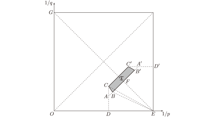
Figure 1. The points $A=(\frac{d+1}{2d},\frac{d-3}{2d})$, $B$, $C$, $D=(\frac{d+1}{2d},0)$, $E=(1,0)$, $F=(\frac{d+2}{2d},\frac{d-2}{2d})$, $G=(0,1)$, $O=(0,0)$, and the dual points $A^{\prime}$, $B^{\prime}$, $C^{\prime}$, $D^{\prime}$ when $d\geq 3$. The line segments $AA^{\prime}$, $CC^{\prime}$, $BE$, and $CE$ are on the lines $\frac{1}{p}-\frac{1}{q}=\frac{2}{d}$, $\frac{1}{p}-\frac{1}{q}=\frac{2}{d+1}$, $\frac{1}{q}=\frac{d-2}{d}(1-\frac{1}{p})$, and $\frac{1}{q}=\frac{d-1}{d+1}(1-\frac{1}{p})$, respectively.

Uniform resolvent estimate. By the reduction in [12] the crucial step for the proof of Theorem 1.1 is to obtain the uniform resolvent estimate

(1.6) $$\|u\|_{L^{q}(\mathbb{R}^{d})}\leq C\|(Q(D)+z)u\|_{L^{p}(\mathbb{R}^{d})},\quad z\in\mathbb{C}$$

for $u\in W^{2,p}(\mathbb{R}^{d}).$ When $Q(D)=\frac{1}{4\pi^{2}}\Delta$, in [12] the resolvent estimates (1.6) were proved for all $p$ and $q$ satisfying the conditions $1/p-1/q=2/d$ and $2d/(d+3)<p<2d/(d+1)$, by making use of the oscillatory integral estimate due to Stein [22]. From these estimates the uniform inequalities (1.2) were obtained in the optimal range of $p$, $q$. These correspond to the open line segment $AA^{\prime}$ in Figure 1. In particular, if $z$ is a positive real number, the estimate is related to Bochner-Riesz operator of order $-1$. The interested reader is referred to [3, 1, 2, 9, 7].

Also, when $Q(D)$ is non-elliptic, Kenig, Ruiz, and Sogge proved that the uniform resolvent estimate

(1.7) $$\|u\|_{L^{q}(\mathbb{R}^{d})}\leq C\|(Q(D)+z)u\|_{L^{p}(\mathbb{R}^{d})},\quad|z|\geq 1$$

is true whenever $1/p+1/q=1$ and $2/(d+1)\leq 1/p-1/q\leq 2/d$ [12, Theorem 2.3]. If $1/p-1/q=2/d$, the uniform estimate (1.7) is equivalent to (1.6) by scaling.

In what follows we extend the known range of $p,q$ for which (1.7) holds. In order to state our result we set

$$B=\Big{(}\frac{d}{2(d-1)},\frac{(d-2)^{2}}{2d(d-1)}\Big{)},\ C=\Big{(}\frac{d+1}{2d},\frac{(d-1)^{2}}{2d(d+1)}\Big{)},$$

and also define $B^{\prime}$ and $C^{\prime}$ by setting $P^{\prime}=(1-y,1-x)$ for $P=(x,y)$ (see Figure 1). Let us denote by $\mathfrak{T}$ the closed trapezoid with vertices $B,B^{\prime},C,C^{\prime}$ from which the points $B,B^{\prime},C,C^{\prime}$ are removed.

Theorem 1.2.

Let $d\geq 3$ and let $Q$ be a non-elliptic, non-degenerate real quadratic form as in Theorem 1.1. Let $(1/p,1/q)\in\mathfrak{T}$. Then there is an absolute constant $C$ such that (1.7) holds with $C$ independent of $z$, $|z|\geq 1$. Furthermore, if $(1/p,1/q)$ is one of the vertices $B,B^{\prime},C,C^{\prime}$, then we have $L^{p,1}$-$L^{q,\infty}$ estimate.

Remark 1.

It was claimed in [2] (Theorem $6^{\prime}$) that the $L^{p}$-$L^{q}$ estimates in Theorem 1.1 were established by combining the interpolation method (Theorem $1^{\prime}$) in [2] and the estimates for the analytic family which are used in [12]. But the argument there does not seem to work. In fact, to show (1.7) by following the lines of argument in [2] (see p.164) one has to consider the analytic family of operators $\{T_{\lambda}\}_{\lambda\in\mathbb{C}}$ which is defined along parameter $\lambda$ by

$$\widehat{T_{\lambda}f}(\xi)=C_{\lambda}(Q(\xi)+z)^{\lambda}\widehat{f}(\xi)$$

with a suitable complex number $C_{\lambda}$ (see [12, 2]). But the crucial assumption $|T_{\lambda}^{*}T_{\lambda}f|\leq C|T_{2\mathop{\mathrm{Re}}\lambda}f|$ of Theorem $1^{\prime}$ is not valid for $T_{\lambda}$. This inequality can not be satisfied for general complex number $z$ unless $z$ is real because

$$T_{\lambda}^{*}T_{\lambda}f=|C_{\lambda}|^{2}\mathcal{F}^{-1}\big{(}{(Q(\xi)+\bar{z})^{\bar{\lambda}}(Q(\xi)+z)^{\lambda}\widehat{f}(\xi)}\big{)}.$$

Restriction-extension operator. The uniform estimates (1.2) and (1.7) are closely related to the $L^{2}$-Fourier restriction estimate to the surfaces $\Sigma_{\rho}=\{\xi:Q(\xi)=\rho\}$. We note that

$$\frac{1}{Q(\xi)\pm 1+i\epsilon}-\frac{1}{Q(\xi)\pm 1-i\epsilon}=\frac{-2i\epsilon}{(Q(\xi)\pm 1)^{2}+\epsilon^{2}}\to-2\pi i\,\delta(Q(\xi)\pm 1)$$

as $\epsilon\to 0$ in the sense of tempered distribution. Here $\delta$ is the delta distribution and $\delta(Q(\xi)\pm\rho)$ is the composition of the distribution $\delta$ with the smooth function $Q(\xi)\pm\rho$. For $\rho\neq 0$, $\delta(Q(\xi)-\rho)$ is well defined. See [10, pp.133–137] for detail. It should be noted that $\delta(Q(\xi)-\rho)$ coincides with the canonical measure on $\Sigma_{\rho}$. Hence, the uniform estimate (1.2) (also (1.6) and (1.7)) implies

(1.8) $$\Big{\|}\int\delta(Q(\xi)\pm 1)e^{2\pi ix\cdot\xi}\widehat{f}(\xi)d\xi\Big{\|}_{L^{q}(\mathbb{R}^{d})}\leq C\|f\|_{L^{p}(\mathbb{R}^{d})},\quad f\in\mathcal{S}(\mathbb{R}^{d}).$$

(Here $\mathcal{S}(\mathbb{R}^{d})$ denotes the Schwartz space.) Instead of the term extension operator which is typically used and somehow misleading we call the operator $f\to\mathcal{F}^{-1}\big{(}{\delta(Q\pm 1)\widehat{f}\,\,}\big{)}$ restriction-extension operator since it is composition of the Fourier restriction and extension (its dual) operators defined by the surface $\Sigma_{\mp 1}$. As is clear to experts, (1.8) is closely related to the inhomogeneous Strichartz estimates. See [11, 8, 27, 25] and references therein. Especially, if $Q(\xi)=-\xi_{1}^{2}+\xi_{2}^{2}+\dots+\xi_{d}^{2}$, (1.8) relates to the estimates for the Klein-Gordon equation. For example, see [17, 18] for earlier results.

By scaling (1.8) implies the estimate

(1.9) $$\Big{\|}\int\delta(Q(\xi)-\rho)e^{2\pi ix\cdot\xi}\widehat{f}(\xi)d\xi\Big{\|}_{L^{q}(\mathbb{R}^{d})}\leq C{|\rho|^{\frac{1}{2}(\frac{d}{p}-\frac{d}{q}-2)}}\|f\|_{L^{p}(\mathbb{R}^{d})},\quad f\in\mathcal{S}(\mathbb{R}^{d}),$$

for $\rho\neq 0$. This estimate will play an important role in proving (1.7). Even if (1.8) is obviously weaker than (1.7), in view of our argument which proves (1.7) the estimate (1.8) may be considered to be almost as strong as (1.7). In Section 3 we show that (1.8) holds for the same $p,q$ as in Theorem 1.2 (see Proposition 3.1).

The rest of this paper is organized as follows. In section 2 we state and prove technical lemmas which decompose the delta and principal value distributions into a sum of functions while these functions possess favorable cancellation properties. These lemmas will be crucial for obtaining the sharp estimates. Also, we show sharp estimates for the multiplier operators associated with the surfaces $\Sigma_{\rho}$. In section 3 we prove the restriction-extension estimate (1.8) and investigate its necessary conditions, which in turn give the optimality of the range of $p,q$ in Theorem 1.1. In section 4 we prove Theorem 1.1 and Theorem 1.2. In section 5, as applications, we shall briefly mention results on Carleman inequalities and unique continuation.

Notations. Throughout this paper the constant $C$ may vary line to line. For $A,B>0$ we write $A\lesssim B$ to denote $A\leq CB$ for some constant $C>0$ independent of $A,B$. By $A\sim B$ we mean $A\lesssim B$ and $B\lesssim A$. Also, $\widehat{f}$ and $f^{\vee}$ denote the Fourier and inverse Fourier transforms of $f$, respectively;

$$\widehat{f}(\xi)=\int_{\mathbb{R}^{d}}e^{-2\pi ix\cdot\xi}f(x)dx,\quad f^{\vee}(x)=\int_{\mathbb{R}^{d}}e^{2\pi ix\cdot\xi}f(\xi)d\xi.$$

We also use the notations $\mathcal{F}(f)$ and $\mathcal{F}^{-1}\big{(}{f}\big{)}$ for the Fourier and the inverse Fourier transforms of $f$, respectively. In the sequel we frequently need to consider points $x,\eta\in\mathbb{R}^{d}$ in separated variables. We write $x=(x_{1},x^{\prime},x^{\prime\prime},x_{d})\in\mathbb{R}\times\mathbb{R}^{k-1}\times\mathbb{R}^{d-k-1}\times\mathbb{R}$ and $\eta=(\eta_{1},\eta^{\prime},\eta^{\prime\prime},\eta_{d})\in\mathbb{R}\times\mathbb{R}^{k-1}\times\mathbb{R}^{d-k-1}\times\mathbb{R}$. We also write as $\tilde{x}=(x_{1},x^{\prime},x^{\prime\prime})\in\mathbb{R}^{d-1}$ and $\tilde{\eta}=(\eta_{1},{\eta^{\prime}},{\eta^{\prime\prime}})\in\mathbb{R}^{d-1}$.

2. Preliminaries

2.1. Decomposition of distributions

We now state and prove the following lemmas which provide dyadic decompositions of the delta and the principal value distributions. These are to be used in Section 3.

Lemma 2.1.

There is a function $\psi\in\mathcal{S}(\mathbb{R})$ of which Fourier transform $\widehat{\psi}$ is supported in $[-2,-1/2]\cup[1/2,2]$ such that, for all $g\in\mathcal{S}(\mathbb{R})$,

$$g(0)=\sum_{j=-\infty}^{\infty}2^{-j}\int\psi(2^{-j}x)g(x)dx.$$

Proof.

The proof of this lemma is rather straightforward. Let $\phi$ be a smooth function supported in $[-2,-1/2]\cup[1/2,2]$ such that $\sum_{j=-\infty}^{\infty}\phi(2^{j}x)=1$ for $x\neq 0$. Then, for $g\in\mathcal{S}(\mathbb{R})$

$$g(0)=\int\widehat{g}(\xi)d\xi=\sum_{j=-\infty}^{\infty}\int\phi(2^{j}\xi)\widehat{g}(\xi)d\xi=\sum_{j=-\infty}^{\infty}\int 2^{-j}\widehat{\phi}(2^{-j}x)g(x)dx.$$

Hence we need only to set $\psi=\widehat{\phi}$. ∎

Lemma 2.2.

There is an odd function $\psi\in\mathcal{S}(\mathbb{R})$ of which Fourier transform $\widehat{\psi}$ is supported in $[-2,-1/2]\cup[1/2,2]$ such that, for all $g\in\mathcal{S}(\mathbb{R})$,

(2.1) $$\operatorname{p.v.}\int\frac{1}{x}\,g(x)dx=\sum_{j=-\infty}^{\infty}2^{-j}\int\psi(2^{-j}x)g(x)dx.$$

Proof.

Let $\chi$ be a smooth function supported in the interval $[1,2]$ satisfying $\int_{\mathbb{R}}\chi(x)dx=1/2$. We set $\widehat{\phi}(\xi)=\chi(\xi)+\chi(-\xi)$ and $\varphi(x)=\phi(x/2)-\phi(x)$. Since $\phi(0)=1$ and $\phi\in\mathcal{S}(\mathbb{R})$, it is easy to see that

$$\sum_{j=-\infty}^{\infty}\varphi(2^{-j}x)=\lim_{\begin{subarray}{c}m\to\infty\\ n\to\infty\end{subarray}}\sum_{j=-m}^{n}\varphi(2^{-j}x)=\lim_{\begin{subarray}{c}m\to\infty\\ n\to\infty\end{subarray}}\big{(}\phi(2^{-n-1}x)-\phi(2^{m}x)\big{)}=1$$

whenever $x\neq 0$. Let us set $\chi_{0}=\chi_{(-1,1)}$ and $\chi_{\infty}=1-\chi_{0}$. Then, for $g\in\mathcal{S}(\mathbb{R})$,

$$\operatorname{p.v.}\int\frac{1}{x}g(x)dx=\int\frac{1}{x}g(x)\chi_{\infty}(x)dx+\int\frac{1}{x}(g(x)-g(0))\chi_{0}(x)dx.$$

Since $\frac{1}{x}g(x)\chi_{\infty}(x)+\frac{1}{x}(g(x)-g(0))\chi_{0}(x)$ is integrable on $\mathbb{R}$, by the dominated convergence theorem we may write

$$\operatorname{p.v.}\int\frac{1}{x}g(x)dx=\sum_{j=-\infty}^{\infty}\int\frac{1}{x}\varphi(2^{-j}x)[g(x)\chi_{\infty}(x)+(g(x)-g(0))\chi_{0}(x)]dx.$$

Since $\varphi(0)=0$ and $\varphi$ is even, $\frac{1}{x}\varphi(2^{-j}x)$ is integrable and $\int\frac{1}{x}\varphi(2^{-j}x)\chi_{0}(x)dx=0$. Thus, we get

$$\operatorname{p.v.}\int\frac{1}{x}g(x)dx=\sum_{j=-\infty}^{\infty}\int\frac{1}{x}\varphi(2^{-j}x)g(x)dx.$$

To get the desired (2.1) we need only to set

$$\psi(x)=\frac{\varphi(x)}{x}.$$

It now remains to show that $\operatorname{supp}\widehat{\psi}\subset[-2,-1/2]\cup[1/2,2]$. Since $\widehat{\psi}(t)=\int e^{-2\pi itx}\frac{\varphi(x)}{x}dx$ it is clear that $\frac{d\widehat{\psi}}{dt}(t)=-2\pi i\widehat{\varphi}(t)$. Hence we may write

(2.2) $$\widehat{\psi}(t)=-2\pi i\int_{-\infty}^{t}\widehat{\varphi}(s)ds=-2\pi i\int_{-\infty}^{t}2\chi(2s)-\chi(s)+2\chi(-2s)-\chi(-s)ds.$$

Since $\chi$ is supported in $[1,2]$, it is easy to check that the integral vanishes if $|t|\geq 2$ or $|t|\leq 1/2$. From this it follows that $\psi\in\mathcal{S}(\mathbb{R})$. ∎

2.2. Estimates associated with the surfaces $\Sigma_{\rho}$

In sections 3 and 4 we shall apply smooth partition of unity and change of coordinates so that the surface $\{\xi:Q(\xi)=\rho\}$ is written locally as the graph of

$$\mathcal{G}_{\rho}(\tilde{\eta})=\frac{|{\eta^{\prime}}|^{2}-|{\eta^{\prime\prime}}|^{2}+\rho}{2\eta_{1}}$$

over the set

$${\mathcal{D}}=\big{\{}\tilde{\eta}=(\eta_{1},\eta^{\prime},\eta^{\prime\prime})\in\mathbb{R}^{d-1}:|{\eta^{\prime}}|\leq 1,|{\eta^{\prime\prime}}|\leq 1,\eta_{1}\in[1,2]\big{\}}.$$

Lemma 2.3.

Let $\mathcal{G}_{\rho}$ be given as in the above and set

$$I(x)=\int e^{{2\pi}i(\tilde{x}\cdot\tilde{\eta}+x_{d}\mathcal{G}_{\rho}(\tilde{\eta}))}\tilde{\chi}(\tilde{\eta})d\tilde{\eta},$$

where $\tilde{\chi}\in C^{\infty}_{c}(\mathcal{D})$. Then, there is a constant $C$, independent of $\rho$, such that

(2.3) $$|I(x)| \leq C(1+{|x_{d}|}{|\rho|})^{-\frac{1}{2}}(1+|x_{d}|)^{-\frac{d-2}{2}}.$$

Proof.

We may assume $\tilde{\chi}(\tilde{\eta})={\phi_{1}(\eta_{1})\phi_{2}(\eta_{1},{\eta^{\prime}},{\eta^{\prime\prime}})}$ with $\phi_{1}\in C^{\infty}(\mathbb{R})$ supported in $[1/2,4]$ and $\phi_{2}\in C^{\infty}(\mathbb{R}^{d-1})$ supported in $\mathcal{D}$. Let us write

$$I(x)=\int e^{2\pi i(x_{1}\eta_{1}+x_{d}\frac{\rho}{2\eta_{1}})}\phi_{1}(\eta_{1})\iint e^{2\pi i(x^{\prime}\cdot\eta^{\prime}+x^{\prime\prime}\cdot\eta^{\prime\prime}+x_{d}\frac{|{\eta^{\prime}}|^{2}-|{\eta^{\prime\prime}}|^{2}}{2\eta_{1}})}\phi_{2}(\eta_{1},{\eta^{\prime}},{\eta^{\prime\prime}})d{\eta^{\prime}}d{\eta^{\prime\prime}}d\eta_{1}.$$

By Plancherel’s theorem the inner integral equals

$$c\Big{(}\frac{\eta_{1}}{|x_{d}|}\Big{)}^{\frac{d-2}{2}}\iint e^{-\pi i\frac{\eta_{1}}{x_{d}}(|y^{\prime}|^{2}-|y^{\prime\prime}|^{2})}\Phi_{\eta_{1}}({{y}^{\prime},{y^{\prime\prime}}})d{y^{\prime}}d{y^{\prime\prime}},$$

where $\Phi_{\eta_{1}}(y^{\prime},y^{\prime\prime})=e^{-\pi i\frac{\eta_{1}}{x_{d}}(|x^{\prime}|^{2}-|x^{\prime\prime}|^{2}+2x^{\prime}\cdot y^{\prime}-2x^{\prime\prime}\cdot y^{\prime\prime})}\mathcal{F}(\phi_{2}(\eta_{1},\cdot,\cdot))(y^{\prime},y^{\prime\prime})$ and $c$ is a constant with $|c|=1$. Hence

$$I(x)=c|x_{d}|^{-\frac{d-2}{2}}\iint\Big{(}\int\eta_{1}^{\frac{d-2}{2}}e^{2\pi i(x_{1}\eta_{1}+x_{d}\frac{\rho}{2\eta_{1}}-\frac{\eta_{1}}{2x_{d}}(|{y^{\prime}}|^{2}-|{y^{\prime\prime}}|^{2}))}\phi_{1}(\eta_{1})\,\,\Phi_{\eta_{1}}({{y^{\prime}},{y^{\prime\prime}}})d\eta_{1}\Big{)}d{y^{\prime}}d{y^{\prime\prime}}.$$

By the van der Corput lemma the inner integral is bounded by $C(1+{|x_{d}|}{|\rho|})^{-\frac{1}{2}}$ (e.g. [23, Corollary in p.334]). Hence the desired bound follows. ∎

Let us consider the evolution operator $U_{\rho}(t)$ which is given by

$$U_{\rho}(t)g(\tilde{x})=\int e^{{2\pi i}(\tilde{x}\cdot\tilde{\eta}+t\mathcal{G}_{\rho}(\tilde{\eta}))}\tilde{\chi}(\tilde{\eta})\,\widehat{g}(\tilde{\eta})d\tilde{\eta}.$$

From (2.3) we have $\|U_{\rho}(t)g\|_{\infty}\lesssim|t|^{-\sigma}|\rho|^{\frac{d-2}{2}-\sigma}\|g\|_{1}$ for $\frac{d-2}{2}\leq\sigma\leq\frac{d-1}{2}$. Using the standard $TT^{*}$ argument (or following the argument in [11]) we have, for $\frac{d-2}{2}\leq\sigma\leq\frac{d-1}{2}$,

(2.4) $$\|U_{\rho}(t)g(\tilde{x})\|_{L^{\frac{2(\sigma+1)}{\sigma}}(dtd\tilde{x})}\lesssim|\rho|^{\frac{1}{2(\sigma+1)}(\frac{d-2}{2}-\sigma)}\|g\|_{2}.$$

In fact, with $\sigma=\frac{d-1}{2}$, $\sigma=\frac{d-2}{2}$ we have the estimates $\|U_{\rho}(t)g(\tilde{x})\|_{L^{\frac{2(d+1)}{d-1}}(dtd\tilde{x})}\lesssim|\rho|^{-\frac{1}{2(d+1)}}\|g\|_{2},$ $\|U_{\rho}(t)g(\tilde{x})\|_{L^{\frac{2d}{d-2}}(dtd\tilde{x})}\lesssim\|g\|_{2}$, respectively. Interpolation of these estimates also gives (2.4).

Let $m$ be a smooth function on $\mathcal{D}$ satisfying

$$\frac{1}{2}\leq m\leq 2.$$

For $\lambda>0$, we define a multiplier operator $\mathcal{T}^{\rho}_{\lambda}$ by

(2.5) $$\widehat{\mathcal{T}^{\rho}_{\lambda}f}(\eta)=\tilde{\chi}(\tilde{\eta}){\psi}\big{(}\lambda^{-1}m(\tilde{\eta})(\eta_{d}-\mathcal{G}_{\rho}(\tilde{\eta}))\big{)}\widehat{f}(\eta),$$

where $\psi\in\mathcal{S}(\mathbb{R})$ and $\tilde{\chi}$ is a smooth function supported in $\mathcal{D}$.

Lemma 2.4.

Let $0<\lambda\leq 1$, $\psi\in\mathcal{S}(\mathbb{R})$ and $\mathcal{T}^{\rho}_{\lambda}$ be defined by (2.5). Then, for $\frac{d-2}{2}\leq\sigma\leq\frac{d-1}{2}$, the estimate

(2.6) $$\|\mathcal{T}^{\rho}_{\lambda}f\|_{\frac{2(\sigma+1)}{\sigma}}\leq C|\rho|^{\frac{1}{2(\sigma+1)}(\frac{d-2}{2}-\sigma)}\lambda^{\frac{1}{2}}\|f\|_{2}$$

holds with the constant $C$ independent of $\rho$ and $\lambda$.

Proof.

Let $\beta$ be a smooth function supported on $[-2,-1/2]\cup[1/2,2]$ and $\beta_{0}$ be a smooth function supported on $[-2,2]$ which satisfy $\beta_{0}(t)+\sum_{j=1}^{\infty}\beta(2^{-j}t)=1$ on $\mathbb{R}.$ By using this, we decompose the operator $\mathcal{T}^{\rho}_{\lambda}$ so that

$$\mathcal{T}^{\rho}_{\lambda}f=\sum_{j=0}^{\infty}\mathcal{T}_{j}f,$$

where $\mathcal{T}_{j}f$, $j\geq 0$, is defined by $\widehat{\mathcal{T}_{0}f}(\eta)={\beta_{0}}\big{(}\lambda^{-1}(\eta_{d}-\mathcal{G}_{\rho}(\tilde{\eta}))\big{)}\widehat{\mathcal{T}^{\rho}_{\lambda}f}(\eta)$ and

$$\widehat{\mathcal{T}_{j}f}(\eta) ={\beta}\big{(}(2^{j}\lambda)^{-1}(\eta_{d}-\mathcal{G}_{\rho}(\tilde{\eta}))\big{)}\widehat{\mathcal{T}^{\rho}_{\lambda}f}(\eta),\quad~{}j\geq 1.$$

So, it suffices to show that, for $j\geq 0$,

(2.7) $$\|\mathcal{T}_{j}f\|_{\frac{2(\sigma+1)}{\sigma}}\lesssim 2^{-j}|\rho|^{\frac{1}{2(\sigma+1)}(\frac{d-2}{2}-\sigma)}\lambda^{\frac{1}{2}}\|f\|_{2}.$$

For $j\geq 1$, by changing variables $\eta_{d}\to\eta_{d}+\mathcal{G}_{\rho}(\tilde{\eta})$, we have

$$\mathcal{T}_{j}f(x)=\int e^{2\pi i\eta_{d}x_{d}}\beta(\frac{\eta_{d}}{2^{j}\lambda})\int e^{2\pi ix\cdot(\tilde{\eta},\mathcal{G}_{\rho}(\tilde{\eta}))}\tilde{\chi}(\tilde{\eta})\psi(\frac{m(\tilde{\eta})\eta_{d}}{\lambda})\widehat{f}(\tilde{\eta},\eta_{d}+\mathcal{G}_{\rho}(\tilde{\eta}))d\tilde{\eta}d\eta_{d}.$$

We observe that the inner integral equals

(2.8) $$U_{\rho}(x_{d})\big{(}\mathcal{F}^{-1}_{\tilde{x}}\big{(}\psi(\frac{m(\cdot)\eta_{d}}{\lambda}){\widehat{f}}(\cdot,\eta_{d}+\mathcal{G}_{\rho}(\cdot))\big{)}\big{)}(\tilde{x}).$$

Here $\mathcal{F}^{-1}_{\tilde{x}}h$ is the inverse Fourier transform of $h$ in $\tilde{x}$. By (2.4) and Plancherel’s theorem, we see that the $L_{x}^{\frac{2(\sigma+1)}{\sigma}}$-norm of (2.8) is bounded by

$$C|\rho|^{\frac{1}{2(\sigma+1)}(\frac{d-2}{2}-\sigma)}\|\psi(\frac{m(\cdot)\eta_{d}}{\lambda})\widehat{f}(\cdot,\eta_{d}+\mathcal{G}_{\rho}(\cdot))\|_{L^{2}(\mathbb{R}^{d-1})}.$$

Thus, using Minkowski’s inequality we get

$$\|\mathcal{T}_{j}f\|_{\frac{2(\sigma+1)}{\sigma}}\lesssim|\rho|^{\frac{1}{2(\sigma+1)}(\frac{d-2}{2}-\sigma)}\int|\beta(\frac{\eta_{d}}{2^{j}\lambda})|\|\psi(\frac{m(\cdot)\eta_{d}}{\lambda})\widehat{f}(\cdot,\eta_{d}+\mathcal{G}_{\rho}(\cdot))\|_{L^{2}(\mathbb{R}^{d-1})}d\eta_{d}.$$

Note that $|\psi(t)|\lesssim|t|^{-2}$ if $|t|\geq 1/2.$ Since $m\sim 1$ and $\operatorname{supp}\beta(2^{-j}\cdot)\subset[2^{j-1},2^{j+1}]$, $|\psi(\frac{m(\tilde{\eta})\eta_{d}}{\lambda})|\lesssim 2^{-2j},$ whenever $\beta(\frac{\eta_{d}}{2^{j}\lambda})\neq 0.$ Using this and the Cauchy-Schwarz inequality, we get, for $j\geq 1$,

$$\|\mathcal{T}_{j}f\|_{\frac{2(\sigma+1)}{\sigma}} \lesssim 2^{-2j}|\rho|^{\frac{1}{2(\sigma+1)}(\frac{d-2}{2}-\sigma)}\int|\beta(\frac{\eta_{d}}{2^{j}\lambda})|\|\widehat{f}(\cdot,\eta_{d}+\mathcal{G}_{\rho}(\cdot))\|_{L^{2}(\mathbb{R}^{d-1})}d\eta_{d}$$

$$\lesssim 2^{-j}|\rho|^{\frac{1}{2(\sigma+1)}(\frac{d-2}{2}-\sigma)}\lambda^{\frac{1}{2}}\left(\int\|\widehat{f}(\cdot,\eta_{d}+\mathcal{G}_{\rho}(\cdot))\|^{2}_{L^{2}(\mathbb{R}^{d-1})}d\eta_{d}\right)^{\frac{1}{2}}.$$

By reversing the change of variables and Plancherel’s theorem, the last integral is clearly bounded by $\|f\|_{2}^{2}$. Hence, we get (2.7) for $j\geq 1$.

Similarly, repeating the same argument one can easily show (2.7) for $j=0$. So, the proof is completed. ∎

In the following lemma we obtain an estimate for the kernel of $\mathcal{T}_{\lambda}^{\rho}$. For this the support property of $\widehat{\psi}$ becomes important in that the estimate (2.9) is no longer true for a general $\psi\in\mathcal{S}(\mathbb{R})$.

Lemma 2.5.

For every $\rho\neq 0$ and $0<\lambda\leq 1$, let $\mathcal{K}_{\lambda}^{\rho}$ be the kernel of $\mathcal{T}_{\lambda}^{\rho}$, i.e.,

$$\mathcal{K}^{\rho}_{\lambda}(x)=\int_{\mathbb{R}^{d}}\psi\big{(}\lambda^{-1}m(\tilde{\eta})(\eta_{d}-\mathcal{G}_{\rho}(\tilde{\eta}))\big{)}\tilde{\chi}(\tilde{\eta})e^{2\pi ix\cdot\eta}d\eta,$$

where $\psi\in\mathcal{S}(\mathbb{R})$ and $\tilde{\chi}$ is a smooth function supported on $\mathcal{D}$. Suppose $\widehat{\psi}$ is supported on $\{t:1/2\leq|t|\leq 2\}$. Then $\mathcal{K}^{\rho}_{\lambda}$ is supported in the set $\{x\in\mathbb{R}^{d}:|x_{d}|\sim\lambda^{-1}\}$ and

(2.9) $$|\mathcal{K}^{\rho}_{\lambda}(x)|\leq C\lambda^{\frac{d}{2}}\min(1,\lambda^{\frac{1}{2}}|\rho|^{-\frac{1}{2}}).$$

Proof.

By inversion we write

$$\psi\big{(}\lambda^{-1}m(\tilde{\eta})(\eta_{d}-\mathcal{G}_{\rho}(\tilde{\eta}))\big{)}=\frac{\lambda}{m(\tilde{\eta})}\int e^{2\pi i\tau(\eta_{d}-\mathcal{G}_{\rho}(\tilde{\eta}))}\widehat{\psi}(\frac{\lambda\tau}{m(\tilde{\eta})})d\tau.$$

Inserting this and making the change of variables $\eta_{d}\to\eta_{d}+\mathcal{G}_{\rho}(\tilde{\eta})$ and taking integration in $\eta_{d}$, we have

$$\mathcal{K}^{\rho}_{\lambda}(x)=\lambda\int\frac{1}{m(\tilde{\eta})}\widehat{\psi}\big{(}\frac{-\lambda x_{d}}{m(\tilde{\eta})}\big{)}e^{{2\pi}i(\tilde{x}\cdot\tilde{\eta}+x_{d}\mathcal{G}_{\rho}(\tilde{\eta}))}\tilde{\chi}(\tilde{\eta})d\tilde{\eta}.$$

Since $\widehat{\psi}$ is supported in $\{|t|\sim 1\}$ and $m\sim 1$ on the support of $\tilde{\chi}$, we may assume $|\lambda x_{d}|\sim 1$ because $\mathcal{K}^{\rho}_{\lambda}(x)=0$ otherwise. Hence we set

$$\chi(\tilde{\eta})=\frac{1}{m(\tilde{\eta})}\widehat{\psi}\big{(}\frac{-\lambda x_{d}}{m(\tilde{\eta})}\big{)}\tilde{\chi}(\tilde{\eta}).$$

Then $\chi(\tilde{\eta})$ is contained in $C_{c}^{\infty}(\mathcal{D})$ uniformly in $x_{d},\lambda$. Hence we may repeat the argument in the proof of Lemma 2.3 to see that

$$\Big{|}\int e^{{2\pi}i(\tilde{x}\cdot\tilde{\eta}+x_{d}\mathcal{G}_{\rho}(\tilde{\eta}))}{\chi}(\tilde{\eta})d\tilde{\eta}\Big{|}\lesssim(1+{|x_{d}|}{|\rho|})^{-\frac{1}{2}}(1+|x_{d}|)^{-\frac{d-2}{2}}.$$

This gives the desired estimate (2.9) because $|\lambda x_{d}|\sim 1$. ∎

Proposition 2.6.

Let $\lambda>0$, $0<|\rho|\lesssim 1$, and $\psi\in\mathcal{S}(\mathbb{R})$ with $\widehat{\psi}$ supported in $[-2,-1/2]\cup[1/2,2]$ and let $\mathcal{T}^{\rho}_{\lambda}$ be defined by (2.5). Then, for $1\leq p\leq 2$ and $\frac{1}{q}=\frac{d-1}{d+1}(1-\frac{1}{p})$,

(2.10) $$\|\mathcal{T}^{\rho}_{\lambda}f\|_{q}\lesssim|\rho|^{-\frac{1}{2}(\frac{1}{p}-\frac{1}{q})}\lambda^{\frac{d}{p}-\frac{d-1}{2}}\|f\|_{p},$$

and, for $1\leq p\leq 2$ and $\frac{1}{q}=\frac{d-2}{d}(1-\frac{1}{p})$,

(2.11) $$\|\mathcal{T}^{\rho}_{\lambda}f\|_{q}\lesssim\lambda^{\frac{d-1}{p}-\frac{d-2}{2}}\|f\|_{p}.$$

Proof.

We may assume $\lambda\leq 1$. Otherwise, the $L^{p}$-$L^{q}$ bound for the multiplier operator is uniformly bounded because the multiplier is smooth and uniformly bounded in $C^{\infty}$. The estimate (2.9) gives the estimates $\|\mathcal{T}^{\rho}_{\lambda}f\|_{\infty}\lesssim\lambda^{\frac{d}{2}}\|f\|_{1}$ and $\|\mathcal{T}^{\rho}_{\lambda}f\|_{\infty}\lesssim\lambda^{\frac{d+1}{2}}|\rho|^{-\frac{1}{2}}\|f\|_{1}$. Then interpolation between the first and (2.6) with $\sigma=\frac{d-2}{2}$ gives (2.11). Similarly we interpolate the second estimate and (2.6) with $\sigma=\frac{d-1}{2}$ to get (2.10). ∎

3. Restriction-extension estimate

In this section we study $L^{p}$-$L^{q}$ boundedness of the operator $f\to\mathcal{F}^{-1}\big{(}{\delta(Q-\rho)\widehat{f}}\big{)}$. In fact, we prove Proposition 3.1 below and investigate the allowable range of $p,q$ on which the operator is bounded from $L^{p}$ into $L^{q}$.

Recall $\Sigma_{\rho}=\{\xi:Q(\xi)=\rho\},\rho\neq 0$ and let $d\sigma_{\rho}$ be the surface measure (induced Lebesgue measure) on $\Sigma_{\rho}$. To begin with, we note that

(3.1) $$\int e^{2\pi ix\cdot\xi}\delta(Q(\xi)-\rho)\widehat{f}(\xi)d\xi=\int_{\Sigma_{\rho}}e^{2\pi ix\cdot\xi}\widehat{f}(\xi)\frac{d\sigma_{\rho}}{|\nabla Q(\xi)|}.$$

Proposition 3.1.

Let $\rho=\pm 1$. Under the same assumption as in Theorem 1.2, we have (1.8) whenever $(1/p,1/q)$ is contained in $\mathfrak{T}$. Additionally, if $(1/p,1/q)=B,C,C^{\prime},$ and $B^{\prime}$, then we have $L^{p,1}$-$L^{q,\infty}$ estimate.

When $Q(D)=\frac{1}{4\pi^{2}}\Delta$ and $\rho$ is negative real number, then (1.9) is an estimate for the Bochner-Riesz operator of order $-1$. $L^{p}$-$L^{q}$ estimates for the Bochner-Riesz operator of negative order have been studied by several authors ([3, 19, 6, 2]). The early results go back as far as Tomas and Stein ([26, 22]). It was shown that (1.9) holds for $p=(2d+2)/(d+3)$ and $q=(2d+2)/(d-1)$, which is equivalent to $L^{(2d+2)/(d+3)}$-$L^{2}$ restriction estimates for the sphere. The estimate (1.9) is now known on the optimal range of $p$ and $q$. That is, for $1\leq p,q\leq\infty$, $Q(D)=\frac{1}{4\pi^{2}}\Delta$ and $\rho=-1$, (1.9) is true if and only if $(1/p,1/q)$ is in the set

$$\Big{\{}\Big{(}\frac{1}{p},\frac{1}{q}\Big{)}\in[0,1]\times[0,1]:\frac{1}{p}-\frac{1}{q}\geq\frac{2}{d+1},\,\,\,\frac{1}{p}>\frac{d+1}{2d},\,\,\,\frac{1}{q}<\frac{d-1}{2d}\Big{\}}.$$

On the other hand, if $Q(D)$ is not the Laplace operator, the inequality (1.8) is known to be true if $p=2d/(d+2)$ and $q=2d/(d-2)$ (the point $F$ in Figure 1), which is due to Strichartz [24]. As is mentioned before, for the special case $Q(\xi)=-\xi_{1}^{2}+\xi_{2}^{2}+\dots+\xi_{2}^{2}$ there are other available estimates [17, 18, 25].

3.1. Proof of Proposition 3.1

We prove Proposition 3.1 by showing the restricted weak type estimates at the endpoints $B$, $B^{\prime}$, $C$, and $C^{\prime}$ in Figure 1. Then real interpolation between these estimates gives the estimate (1.8) for $(\frac{1}{p},\frac{1}{q})\in\mathfrak{T}$. By duality it is sufficient to show that, for $(1/p,1/q)=B,$ $C$,

(3.2) $$\|\mathcal{F}^{-1}\big{(}\delta(Q\pm 1)\widehat{f}\,\big{)}\|_{q,\infty}\leq C\|f\|_{p,1}.$$

Let us define the projection operator $P_{j}$, $j\in\mathbb{Z}$, by

$$\widehat{P_{j}f}(\xi)=\beta(2^{-j}|\xi|)\widehat{f}(\xi),$$

where $\beta:\mathbb{R}_{+}\to[0,1]$ is a smooth function supported on the interval $[1/2,2]$ satisfying $\sum_{j=-\infty}^{\infty}\beta(2^{-j}t)=1$ for $t>0$. Since $1<p\leq 2\leq q<\infty$, by Littlewood-Paley theory and Minkowski inequality it is sufficient to show

(3.3) $$\|\mathcal{F}^{-1}\big{(}\delta(Q\pm 1)\widehat{P_{j}f}\,\big{)}\|_{q,\infty}\leq C\|P_{j}f\|_{p,1}.$$

To see this we need the following simple lemma.

Lemma 3.2.

Let $1<p<\infty$, $1\leq r\leq\infty$, and let $L^{p,r}$ denote the Lorentz spaces. Then

$$\|f\|_{p,r}\lesssim\|(\sum|P_{j}f|^{2})^{\frac{1}{2}}\|_{p,r}\lesssim\|f\|_{p,r}.$$

The upper bound follows from the usual Littlewood-Paley inequality $\|(\sum|P_{j}f|^{2})^{\frac{1}{2}}\|_{p}\lesssim\|f\|_{p}$, $1<p<\infty$ and (real) interpolation. Once the upper bound is obtained, the lower bound can be shown by using the usual polarization argument. For example, see [21] or [13] for detail.

Hence, in particular

$$\|\mathcal{F}^{-1}\big{(}{\delta(Q\pm 1)\widehat{f}\,}\big{)}\|_{q,\infty}\sim\Big{\|}\Big{(}\sum_{j}|\mathcal{F}^{-1}\big{(}{\delta(Q\pm 1)\widehat{P_{j}f}\,}\big{)}|^{2}\Big{)}^{1/2}\Big{\|}_{q,\infty}.$$

Since $q>2$, $L^{q/2,\infty}$ is normable. So, we have for $2<q<\infty$

(3.4) $$\|(\sum_{j}|h_{j}|^{2})^{\frac{1}{2}}\|_{q,\infty}\lesssim(\sum_{j}\|h_{j}\|^{2}_{q,\infty})^{\frac{1}{2}}.$$

Combining this with the above inequality gives

$$\|\mathcal{F}^{-1}\big{(}{\delta(Q\pm 1)\widehat{f}\,}\big{)}\|_{q,\infty} \lesssim\Big{(}\sum_{j}\|\mathcal{F}^{-1}\big{(}\delta(Q\pm 1)\widehat{P_{j}f}\,\big{)}\|_{q,\infty}^{2}\Big{)}^{1/2}.$$

We now use (3.3) to get

$$\|\mathcal{F}^{-1}\big{(}{\delta(Q\pm 1)\widehat{f}\,}\big{)}\|_{q,\infty}\lesssim\Big{(}\sum_{j}\|P_{j}f\|_{p,1}^{2}\Big{)}^{1/2}.$$

Since $\|g\|_{r,s}=\sup_{\|h\|_{r^{\prime},s^{\prime}}\leq 1}|\int g(x)h(x)dx|$ for $1\leq r,s\leq\infty$, by the standard duality argument one can easily see that (3.4) implies $(\sum_{j}\|h_{j}\|^{2}_{p,1})^{\frac{1}{2}}\lesssim\|(\sum_{j}|h_{j}|^{2})^{\frac{1}{2}}\|_{p,1}$ if $1<p<2$. Hence we have

$$\|\mathcal{F}^{-1}\big{(}{\delta(Q\pm 1)\widehat{f}\,}\big{)}\|_{q,\infty}\lesssim\Big{\|}(\sum_{j}|P_{j}f|^{2})^{1/2}\Big{\|}_{p,1}.$$

Now Lemma 3.2 gives (3.2). Therefore we are reduced to showing (3.3).

Note that we may assume $2^{j}\geq 2^{-2}$ because $\mathcal{F}^{-1}\big{(}{\delta(Q\pm 1)\widehat{P_{j}f}\,}\big{)}=0$, otherwise. Let us set

$$\mathbb{A}=\{\xi\in\mathbb{R}^{d}:1/2\leq|\xi|\leq 2\}.$$

Then by scaling, (3.3) is equivalent to

(3.5) $$\|\mathcal{F}^{-1}\big{(}\delta(Q\pm 2^{-2j})\widehat{f}\,\big{)}\|_{q,\infty}\leq C2^{j(2-\frac{d}{p}+\frac{d}{q})}\|f\|_{p,1},\quad\operatorname{supp}\widehat{f}\subset\mathbb{A}.$$

By finite decomposition of $\widehat{f}$, we may assume that $\widehat{f}$ is supported in a small neighborhood of a point $\xi_{0}\in\mathbb{A}$. For every invertible linear map $L$ defined on $\mathbb{R}^{d}$ with $|\det L|=1$, the change of variable $\xi\to L\xi$ in the frequency domain is harmless. Specifically, we apply a rotation $R=R_{1}\oplus R_{2}\in SO(\mathbb{R}^{d})$, where $R_{1}\in SO(\mathbb{R}^{k})$ and $R_{2}\in SO(\mathbb{R}^{d-k})$ by splitting the variable $\xi=(\xi_{1},\xi^{\prime},\xi^{\prime\prime},\xi_{d})\in\mathbb{R}^{k}\times\mathbb{R}^{d-k}$ so that the support of $\widehat{f}$ is contained in a small neighborhood (in $\mathbb{R}^{d}$) of the intersection of $\{\xi:Q(\xi)=\mp 2^{-2j},~{}1/2\leq|\xi|\leq 2,~{}{\xi_{1}\geq 0,~{}\xi_{d}\geq 0}\}$ and the $\xi_{1}\xi_{d}$-plane. Since $Q(R\xi)=Q(\xi)$, the surface $\{\xi:Q(\xi)=\mp 2^{-2j}\}$ and the measure $\delta(Q(\xi)\pm 2^{-2j})d\xi=\frac{d\sigma_{\mp 2^{-2j}}}{|\nabla Q(\xi)|}$ are invariant under the rotation $R$. We may assume that the surface is given by

(3.6) $$\mp\,2^{-2j}=Q(\xi)=(\xi_{d}+\xi_{1})(\xi_{d}-\xi_{1})-\xi_{2}^{2}-\cdots-\xi_{k}^{2}+\xi_{k+1}^{2}+\cdots+\xi_{d-1}^{2},$$

and that $\widehat{f}$ is supported on the set

$$\{\xi\in\mathbb{R}^{d}:|\xi_{d}+\xi_{1}|\sim 1,\,|\xi_{d}-\xi_{1}|\lesssim 1,\,|\xi^{\prime}|\ll 1,\,|\xi^{\prime\prime}|\ll 1\}.$$

Next we apply another harmless change of variables via the rotation $\xi\to\eta$, where

(3.7) $$\left\{\begin{array}[]{l}\eta_{1}=(\xi_{d}+\xi_{1})/\sqrt{2},\quad\eta_{d}=(\xi_{d}-\xi_{1})/\sqrt{2},\\ {\eta^{\prime}}={\xi^{\prime}},\ {\eta^{\prime\prime}}={\xi^{\prime\prime}}.\end{array}\right.$$

As mentioned in the introduction, for notational convenience we write $\tilde{\eta}=(\eta_{1},{\eta^{\prime}},{\eta^{\prime\prime}})=(\eta_{1},\cdots,\eta_{d-1})\in\mathbb{R}^{d-1}$. Then the surface given by (3.6) is now represented locally as the graph of $\mathcal{G}_{\mp 2^{-2j}}$ in the new coordinate. For the rest of this section we set

$$\rho=\mp 2^{-2j}.$$

Hence, by change of variables, (3.5) is again equivalent to the estimate

(3.8) $$\Big{\|}\int\delta({\eta_{d}-\mathcal{G}_{\rho}(\tilde{\eta})})e^{2\pi ix\cdot\eta}\widehat{f}(\eta)\chi(\eta)d\eta\Big{\|}_{L^{q,\infty}(\mathbb{R}^{d})}\leq C|\rho|^{\frac{1}{2}(\frac{d}{p}-\frac{d}{q}-2)}\|f\|_{L^{p,1}(\mathbb{R}^{d})},$$

where $\chi$ is a smooth function supported in a set $\mathbb{A}_{0}:=\mathbb{A}\cap\{\eta\in\mathbb{R}^{d}:|{\eta^{\prime}}|\ll 1,~{}|{\eta^{\prime\prime}}|\ll 1,|\eta_{d}|\lesssim 1,~{}\eta_{1}\sim 1\}.$ We now use Lemma 2.1 to get

$$\mathcal{F}^{-1}\big{(}{\delta({\eta_{d}-\mathcal{G}_{\rho}(\tilde{\eta})})\widehat{f}(\eta)\chi(\eta)}\big{)}=\sum_{l\in\mathbb{Z}}T_{l}f,$$

where $\psi$ is a smooth function with $\operatorname{supp}\widehat{\psi}\subset\{t\in\mathbb{R}:|t|\sim 1\}$ and

$$T_{l}f(x)=2^{-l}\int_{\mathbb{R}^{d}}\psi(2^{-l}(\eta_{d}-\mathcal{G}_{\rho}(\tilde{\eta})))\chi(\eta)\widehat{f}(\eta)e^{2\pi ix\cdot\eta}d\eta.$$

3.1.1. Restricted weak type estimate at $B$

By Proposition 2.6 with $m=1$ we have, for $1\leq p\leq 2$ and $\frac{1}{q}=\frac{d-2}{d}(1-\frac{1}{p})$,

(3.9) $$\|{T}_{l}f\|_{q}\lesssim 2^{l(\frac{d-1}{p}-\frac{d}{2})}\|f\|_{p}.$$

Now we make use of the following elementary lemma which was implicit in [4]. A statement in more general setting can also be found in [5].

Lemma 3.3.

Let $\varepsilon_{0},\varepsilon_{1}>0$, and let $\{T_{l}:l\in\mathbb{Z}\}$ be a sequence of linear operators satisfying

$$\|T_{l}f\|_{q_{0}}\leq M_{0}2^{\varepsilon_{0}{l}}\|f\|_{p_{0}},\quad\|T_{l}f\|_{q_{1}}\leq M_{1}2^{-\varepsilon_{1}{l}}\|f\|_{p_{1}}$$

for some $1\leq p_{0},p_{1},q_{0},q_{1}\leq\infty$. Then $T=\sum_{l\in\mathbb{Z}}T_{l}$ is bounded from $L^{p,1}$ to $L^{q,\infty}$ with $\|Tf\|_{q,\infty}\leq CM_{0}^{\theta}M_{1}^{1-\theta}\|f\|_{p,1},$ where $\theta=\varepsilon_{1}/(\varepsilon_{0}+\varepsilon_{1})$, $1/q=\theta/q_{0}+(1-\theta)/q_{1}$, $1/p=\theta/p_{0}+(1-\theta)/p_{1}$.

We choose $(p_{i},q_{i})$ satisfying $\frac{1}{q_{i}}=\frac{d-2}{d}(1-\frac{1}{p_{i}})$ for $i=0,1$, and $\frac{1}{2}\leq\frac{1}{p_{0}}<\frac{d}{2(d-1)}<\frac{1}{p_{1}}<1$. Then by (3.9) we have for $i=0,1,$

$$\|T_{l}f\|_{q_{i}}\leq C2^{l(\frac{d-1}{p_{i}}-\frac{d}{2})}\|f\|_{p_{i}}.$$

Note that $\frac{d}{2}-\frac{d-1}{p_{1}}<0<\frac{d}{2}-\frac{d-1}{p_{0}}$. We combine two estimates for $i=0,1$ and Lemma 3.3 with $\varepsilon_{0}=\frac{d}{2}-\frac{d-1}{p_{0}}$ and $\varepsilon_{1}=-\frac{d}{2}+\frac{d-1}{p_{1}}$ to get

$$\|\mathcal{F}^{-1}\big{(}{\delta({\eta_{d}-\mathcal{G}_{\rho}(\tilde{\eta})})\widehat{f}(\eta)\chi(\eta)}\big{)}\|_{q,\infty}\leq C\|f\|_{p,1}$$

for $(1/p,1/q)=B$. This is (3.8) when $(1/p,1/q)=B$.

3.1.2. Restricted weak type estimate at $C$

Again by proposition 2.6 we have, for $1\leq p\leq 2$ and $\frac{1}{q}=\frac{d-1}{d+1}(1-\frac{1}{p})$,

$$\|{T}_{l}f\|_{q}\lesssim|\rho|^{-\frac{1}{2}(\frac{1}{p}-\frac{1}{q})}2^{l(\frac{d}{p}-\frac{d+1}{2})}\|f\|_{p}.$$

By the same argument as before we get the restricted weak type estimate

$$\|\mathcal{F}^{-1}\big{(}{\delta({\eta_{d}-\mathcal{G}_{\rho}(\tilde{\eta})})\widehat{f}(\eta)\chi(\eta)}\big{)}\|_{q,\infty}\lesssim|\rho|^{-\frac{1}{2}(\frac{1}{p}-\frac{1}{q})}\|f\|_{p,1}$$

for $(1/p,1/q)=C$. Finally note that $|\rho|^{-\frac{1}{2}(\frac{1}{p}-\frac{1}{q})}=|\rho|^{\frac{1}{2}(\frac{d}{p}-\frac{d}{q}-2)}$ when $(1/p,1/q)=C$. Hence we have (3.8) for $(1/p,1/q)=C$.

3.2. Estimate for $f\to\mathcal{F}^{-1}\big{(}{\psi(2^{-l}(Q-a))\widehat{f}\,\,}\big{)}$

In this section we prove a few estimates which will be used later.

Proposition 3.4.

Let $\lambda>0$, $0<|a|\lesssim 1$, $\psi\in\mathcal{S}(\mathbb{R})$ with $\widehat{\psi}$ supported in $[-2,-1/2]\cup[1/2,2]$. Then, if the support of Fourier transform of $f$ is contained in $\{\xi:|\xi|\geq 1/2\}$, for $1<p\leq 2$ and $\frac{1}{q}=\frac{d-1}{d+1}(1-\frac{1}{p})$,

(3.10) $$\|\mathcal{F}^{-1}\big{(}{\psi(\lambda^{-1}(Q-a))\widehat{f}\,\,}\big{)}\|_{q}\lesssim|a|^{-\frac{1}{2}(\frac{1}{p}-\frac{1}{q})}\lambda^{\frac{d}{p}-\frac{d-1}{2}}\|f\|_{p},$$

and, for $1<p\leq 2$ and $\frac{1}{q}=\frac{d-2}{d}(1-\frac{1}{p})$,

(3.11) $$\|\mathcal{F}^{-1}\big{(}{\psi(\lambda^{-1}(Q-a))\widehat{f}\,\,}\big{)}\|_{q}\lesssim\lambda^{\frac{d-1}{p}-\frac{d-2}{2}}\|f\|_{p}.$$

In order to show this, by Littlewood-Paley inequality and using the fact that $1<p\leq 2\leq q<\infty$, it is sufficient to obtain (3.10) and (3.11) for the same $p,q$ as in Proposition 3.4 with $f$ of which Fourier transform is supported $\{\xi:2^{j-1}\leq|\xi|\leq 2^{j+1}\}$, $j\geq-1$. The estimates for each dyadic piece can be put together by the same argument as before. By rescaling it is enough to do this with $f$ whose Fourier transform is supported in $\mathbb{A}$. In fact, by rescaling ($\xi\to 2^{j}\xi$ in frequency domain) we have

$$\mathcal{F}^{-1}\big{(}{\psi(\lambda^{-1}(Q-a))\widehat{f}\,\,}\big{)}(x)=\mathcal{F}^{-1}\big{(}{\psi((2^{-2j}\lambda)^{-1}(Q-2^{-2j}a))\widehat{f(2^{-j}\cdot)}}\big{)}(2^{j}x).$$

Since $\widehat{f(2^{-j}\cdot)}$ is supported in $\mathbb{A}$, we see that (3.10) and (3.11) with $\widehat{f}$ supported in $\mathbb{A}$ implies

$$\|\mathcal{F}^{-1}\big{(}{\psi(\lambda^{-1}(Q-a))\widehat{f}\,\,}\big{)}\|_{q} \lesssim 2^{j((d-1)(1-\frac{1}{p})-\frac{d+1}{q})}|a|^{-\frac{1}{2}(\frac{1}{p}-\frac{1}{q})}\lambda^{\frac{d}{p}-\frac{d-1}{2}}\|f\|_{p},$$

$$\|\mathcal{F}^{-1}\big{(}{\psi(\lambda^{-1}(Q-a))\widehat{f}\,\,}\big{)}\|_{q} \lesssim 2^{j((d-2)(1-\frac{1}{p})-\frac{d}{q})}\lambda^{\frac{d-1}{p}-\frac{d-2}{2}}\|f\|_{p},$$

respectively, provided that the Fourier transform of $f$ is supported in $\{\xi:2^{j-1}\leq|\xi|\leq 2^{j+1}\}$, $j\geq-1$. Therefore, for the proof of Proposition 3.4 it is sufficient to show (3.10) with $\widehat{f}$ supported in $\mathbb{A}$ and $0<|a|\lesssim 1$ for $1<p\leq 2$ and $\frac{1}{q}=\frac{d-1}{d+1}(1-\frac{1}{p})$, and (3.11) for $1<p\leq 2$ and $\frac{1}{q}=\frac{d-2}{d}(1-\frac{1}{p})$.

Since $Q$ is non-elliptic, by finite decomposition of the support of $\widehat{f}$, rotation and changing variables ((3.6), (3.7)), to show (3.10) and (3.11) with $\widehat{f}$ supported in $\mathbb{A}$, it is sufficient to show the same bounds for $\mathcal{F}^{-1}\big{(}{\psi(\lambda^{-1}(2\eta_{1}(\eta_{d}-\mathcal{G}_{a}(\tilde{\eta})))\tilde{\chi}\,\widehat{f}\,\,}\big{)}$ instead of $\mathcal{F}^{-1}\big{(}{\psi(\lambda^{-1}(Q-a))\widehat{f}\,\,}\big{)}$ while $\widehat{f}$ is assumed to be supported in $\mathbb{A}_{0}$. This can easily be done by repeating the proof of Proposition 2.6 by using Lemma 2.4 and Lemma 2.5 with $m(\tilde{\eta})=2\eta_{1}$. This completes the proof.

3.3. Bounds for the multiplier given by principal value

Let us consider the estimate

(3.12) $$\Big{\|}\mathcal{F}^{-1}\Big{(}\operatorname{p.v.}\frac{1}{Q(\xi)\pm 1}\widehat{f}(\xi)\Big{)}\Big{\|}_{q}\leq C\|f\|_{p}.$$

We now have another result similar to Proposition 3.1.

Proposition 3.5.

Let $d\geq 3$ and let $Q$ be a non-elliptic quadratic form as in Theorem 1.1. Let $(1/p,1/q)$ be contained in $\mathfrak{T}$. Then there is a constant $C$ such that (3.12) holds. Additionally, if $(1/p,1/q)=B,C,C^{\prime},$ and $B^{\prime}$, then we have $L^{p,1}$-$L^{q,\infty}$ estimate.

This can be proved by the same argument which is used for the proof of Proposition 3.1. So, we shall be brief. The distribution $\operatorname{p.v.}\frac{1}{Q(\xi)\pm 1}$ is smooth on $|\xi|<3/4$ and bounded away from zero. So, we may assume $\widehat{f}$ is supported in $\{\xi:|\xi|\geq 1/2\}$. As before, by Littlewood-Paley theory and scaling it is enough to show that, for $(1/p,1/q)=B,C,$ and $j\geq 0$

$$\Big{\|}\mathcal{F}^{-1}\Big{(}\operatorname{p.v.}\frac{1}{Q(\xi)\pm 2^{-2j}}\widehat{f}(\xi)\Big{)}\Big{\|}_{q,\infty}\leq C2^{j(2-\frac{d}{p}+\frac{d}{q})}\|f\|_{p,1},\quad\operatorname{supp}\widehat{f}\subset\mathbb{A}.$$

Let us set $\rho=\mp 2^{-2j}$ as before. By finite decomposition, rotation, and change of variables (3.6) and (3.7), this further reduces to showing the estimate

(3.13) $$\Big{\|}\mathcal{F}^{-1}\Big{(}\operatorname{p.v.}\frac{1}{\eta_{d}-\mathcal{G}_{\rho}(\tilde{\eta})}\tilde{\chi}(\tilde{\eta})\widehat{f}(\eta)\Big{)}\Big{\|}_{q,\infty}\leq C{|\rho|^{\frac{1}{2}(\frac{d}{p}-\frac{d}{q}-2)}}\|f\|_{p,1},\quad\operatorname{supp}\widehat{f}\subset\mathbb{A}_{0},$$

where $\tilde{\chi}$ is smooth function supported in $\mathcal{D}$. Now, by Lemma 2.2, we decompose this operator as

$$\mathcal{F}^{-1}\Big{(}\operatorname{p.v.}\frac{1}{\eta_{d}-\mathcal{G}_{\rho}(\tilde{\eta})}\tilde{\chi}(\tilde{\eta})\widehat{f}(\eta)\Big{)}=\sum_{l\in\mathbb{Z}}2^{-l}\int_{\mathbb{R}^{d}}\psi(2^{-l}(\eta_{d}-\mathcal{G}_{\rho}(\tilde{\eta})))\tilde{\chi}(\tilde{\eta})\widehat{f}(\eta)e^{2\pi ix\cdot\eta}d\eta,$$

where $\psi$ is a smooth function on $\mathbb{R}$ such that $\operatorname{supp}\widehat{\psi}\subset\{t\in\mathbb{R}:|t|\sim 1\}$. At this point we remark that the exactly same argument as in Section 3.1 can be applied to show (3.13) for $(1/p,1/q)=B$, or $C$. So we avoid duplication.

3.4. Necessary conditions

In this section we obtain necessary conditions for the estimates (1.2), (1.6), (1.8). By the implication (1.2) $\rightarrow$ (1.6) $\rightarrow$ (1.8) it is sufficient to consider (1.8).

3.4.1. Failure of (1.8) for $\frac{1}{p}-\frac{1}{q}>\frac{2}{d}$

After change of variables (3.6), (3.7), the quadratic form $Q$ is replaced by $2\eta_{1}\eta_{d}-|\eta^{\prime}|^{2}+|\eta^{\prime\prime}|^{2}$. By (3.1) it follows that the estimate (1.8) implies

(3.14) $$\Big{\|}\int e^{2\pi i(\tilde{x}\cdot\tilde{\eta}+x_{d}\mathcal{G}_{\pm 1}(\tilde{\eta}))}\widehat{g}(\tilde{\eta},\mathcal{G}_{\pm 1}(\tilde{\eta}))\frac{1}{2\eta_{1}}d\tilde{\eta}\Big{\|}_{L^{q}(\mathbb{R}^{d})}\leq C\|g\|_{L^{p}(\mathbb{R}^{d})},$$

whenever $\widehat{g}$ vanishes near $\eta_{1}=0.$ Let $\phi\in C_{c}^{\infty}(\mathbb{R})$ be supported on the interval $[-2^{-2},2^{-2}]$. For $0<\lambda\ll 1$, define $g_{\lambda}\in\mathcal{S}(\mathbb{R}^{d})$ by

(3.15) $$\widehat{g_{\lambda}}(\eta)=\phi(\lambda^{2}(\eta_{1}-\lambda^{-2}))\phi(\eta_{d})\prod_{j=2}^{d-1}\phi(\lambda\eta_{j}).$$

Since $\widehat{g_{\lambda}}$ is supported in the $d$-dimensional rectangle

$$R_{\lambda}=\{\eta\in\mathbb{R}^{d}:|\eta_{1}-\lambda^{-2}|\leq(2\lambda)^{-2},~{}|\eta_{d}|\leq 2^{-2},~{}|\eta_{j}|\leq({4\lambda})^{-1},~{}2\leq j\leq d-1\},$$

it is easy to see that $\big{|}\int e^{2\pi i(\tilde{x}\cdot\tilde{\eta}+x_{d}\mathcal{G}_{\pm 1}(\tilde{\eta}))}\widehat{g_{\lambda}}(\tilde{\eta},\mathcal{G}_{\pm 1}(\tilde{\eta}))\frac{1}{2\eta_{1}}d\tilde{\eta}\big{|}\gtrsim\lambda^{2}|{R_{\lambda}}|$ if $x$ is in the set

$$R_{\lambda}^{\prime}=\big{\{}x\in\mathbb{R}^{d}:|x_{1}|\leq\frac{\lambda^{2}}{125d},~{}|x_{d}|\leq\frac{1}{20d},~{}|x_{j}|\leq\frac{\lambda}{25d},~{}2\leq j\leq d-1\big{\}}.$$

Hence, we have

$$\Big{\|}\int e^{2\pi i(\tilde{x}\cdot\tilde{\eta}+x_{d}\mathcal{G}_{\pm 1}(\tilde{\eta}))}\widehat{g_{\lambda}}(\tilde{\eta},\mathcal{G}_{\pm 1}(\tilde{\eta}))\frac{1}{2\eta_{1}}d\tilde{\eta}\Big{\|}_{L^{q}(R_{\lambda}^{\prime})}\gtrsim\lambda^{2}|{R_{\lambda}}||R_{\lambda}^{\prime}|^{1/q}\sim\lambda^{2-d+d/q}.$$

On the other hand it is also clear that $\|g_{\lambda}\|_{p}\lesssim\lambda^{-d+d/p}$. Therefore, (3.14) gives $\lambda^{2-d+d/q}\lesssim\lambda^{-d+d/p}$. By letting $\lambda\to 0$ we see that the inequality (1.8) cannot be true unless $1/p-1/q\leq 2/d$.

3.4.2. Failure of (1.8) for $\frac{1}{p}-\frac{1}{q}<\frac{2}{d+1}$, $q{~{}\leq~{}}\frac{2d}{d-1}$, $p{~{}\geq~{}}\frac{2d}{d+1}$

Failure of (1.8) on this range can be shown similarly as in the proof of Bochner-Riesz means of negative order (see [3] [7]). Here we only consider the case $\delta(Q-1)$. The other case $\delta(Q+1)$ can be shown via a little modification.

Typical Knapp’s example shows the estimate (1.8) is only possible for

(3.16) $$\frac{1}{p}-\frac{1}{q}\geq\frac{2}{d+1}.$$

In fact, for $0<\lambda\ll 1$, let us define $\widehat{f_{\lambda}}(\xi)=\phi(\lambda^{-2}(\xi_{d}-1))\prod_{j=1}^{d-1}\phi(\lambda^{-1}\xi_{j})$, where $\phi\in C^{\infty}_{c}(\mathbb{R})$ is the same function as in (3.15). Then it is easy to see that

$$\Big{|}\int\delta(Q(\xi)-1)e^{2\pi ix\cdot\xi}\widehat{f_{\lambda}}(\xi)d\xi\Big{|}\gtrsim\lambda^{d-1}$$

for $|x_{d}|\leq c\lambda^{-2}$ and $|x_{j}|\leq c\lambda^{-1},\,j\neq d$ with a sufficiently small $c>0$. The estimate (1.8) implies $\lambda^{d-1}\lambda^{-\frac{d+1}{q}}\lesssim\lambda^{d+1-\frac{d+1}{p}}$. Letting $\lambda\to 0$ gives the condition (3.16).

The surface $\{\xi:Q(\xi)=1,\ |\xi|\leq 2\}$ has nonvanishing Gaussian curvature. If we choose a function $f$ with $\widehat{f}$ supported in a small enough neighborhood of $(0,\pm 1)\in\mathbb{R}^{d-1}\times\mathbb{R}$, then by the stationary phase method we see

$$\Big{|}\int\delta(Q(\xi)\,-\,1)e^{2\pi ix\cdot\xi}\widehat{f}(\xi)d\xi\Big{|}\gtrsim|{x_{d}}|^{\frac{1-d}{2}}$$

if $c|x_{d}|>|\tilde{x}|$. The estimate (1.8) implies that $|{x_{d}}|^{\frac{1-d}{2}}\chi_{\{c|x_{d}|>|\tilde{x}|\}}\in L^{q}$. Hence, it follows that $\frac{(d-1)q}{2}>d$ and the estimate (1.8) can not be true for $q{~{}\leq~{}}\frac{2d}{d-1}$. Duality gives the other condition $p{~{}\geq~{}}\frac{2d}{d+1}$.

3.4.3. Necessity of the condition $p<2(d-1)/d,~{}q>2(d-1)/(d-2)$ for (1.8) when $1/p-1/q=2/d$

It is enough to show $q>2(d-1)/(d-2)$ because of duality.

Let $m_{1}<m_{2}$ be positive numbers. From scaling, we see that (1.8) implies for any $r>0$

$$\Big{\|}\int\delta(Q(\xi)-r^{2})e^{2\pi ix\cdot\xi}\widehat{f}(\xi)d\xi\Big{\|}_{L^{q}(\mathbb{R}^{d})}\leq C\|f\|_{L^{p}(\mathbb{R}^{d})}$$

with $C$ independent of $m_{1},m_{2}$ if $\operatorname{supp}\widehat{f}\subset\{\xi:m_{1}\leq|\xi|\leq m_{2}\}$ and $1/p-1/q=2/d$. Letting $r\to 0$ gives, for $\operatorname{supp}\widehat{f}\subset\{\xi:m_{1}\leq|\xi|\leq m_{2}\}$,

(3.17) $$\Big{\|}\int\delta(Q(\xi))e^{2\pi ix\cdot\xi}\widehat{f}(\xi)d\xi\Big{\|}_{L^{q}(\mathbb{R}^{d})}\leq C\|f\|_{L^{p}(\mathbb{R}^{d})}.$$

Then parameterizing the set $\{\xi:Q(\xi)=0\}$, in particular, we see that (3.17) implies

(3.18) $$\Big{\|}\int_{\mathbb{R}^{d-1}}\widehat{g}\Big{(}\tilde{\eta},\frac{|{\eta^{\prime}}|^{2}-|{\eta^{\prime\prime}}|^{2}}{2\eta_{1}}\Big{)}e^{2\pi i(\tilde{x}\cdot\tilde{\eta}+x_{d}\frac{|{\eta^{\prime}}|^{2}-|{\eta^{\prime\prime}}|^{2}}{2\eta_{1}})}\tilde{\chi}(\tilde{\eta})d\tilde{\eta}\Big{\|}_{q}\leq C\|g\|_{p}$$

whenever $\tilde{\chi}$ is a smooth function supported in $\{\tilde{\eta}:\eta_{1}\in(10^{-2},10^{2}),|(\eta^{\prime},\eta^{\prime\prime})|\leq M\}$ for any $M>0$. Here we use the same coordinates given by (3.7). Let $\phi\in C^{\infty}_{c}(-10^{-2},10^{-2})$ be satisfying

$$0\leq\widehat{\phi}(t)\leq 2~{}\text{for ~{} all }~{}t\in\mathbb{R}\quad\text{and}\quad\widehat{\phi}(t)\geq 1~{}\text{on}~{}|t|\leq 1.$$

Also, let $\phi_{2}\in C^{\infty}_{c}(\mathbb{R}^{k-1})$ and $\phi_{3}\in C^{\infty}_{c}(\mathbb{R}^{d-k-1})$ be radial functions which are supported in the balls $B(0,M/2)$ and have nonnegative Fourier transforms. We set

$$\phi_{1}(t)=t^{\frac{-d+2}{2}}\phi(t-1),\ \tilde{\chi}(\tilde{\eta})=\phi_{1}(\eta_{1})\phi_{2}({\eta^{\prime}})\phi_{3}({\eta^{\prime\prime}}).$$

From the support condition, the inequality (3.18) holds for such $\tilde{\chi}$. Choose $g\in\mathcal{S}(\mathbb{R}^{d})$ such that $|\widehat{g}\Big{(}\tilde{\eta},\frac{|{\eta^{\prime}}|^{2}-|{\eta^{\prime\prime}}|^{2}}{2\eta_{1}}\Big{)}|\equiv 1$ if $\tilde{\eta}\in\operatorname{supp}\tilde{\chi}$. Then (3.18) implies that

$$K(x)=\int_{\mathbb{R}^{d-1}}e^{2\pi i(\tilde{x}\cdot\tilde{\eta}+x_{d}\frac{|{\eta^{\prime}}|^{2}-|{\eta^{\prime\prime}}|^{2}}{2\eta_{1}})}\phi_{1}(\eta_{1})\phi_{2}({\eta^{\prime}})\phi_{3}({\eta^{\prime\prime}})d\tilde{\eta}$$

is in $L^{q}(\mathbb{R}^{d})$.

We now compute $K$. By making use of the Fourier transform of the Gaussian function, we obtain, for $x_{d}\neq 0$,

$$K(x) =|x_{d}|^{-\frac{d-2}{2}}e^{\pi i\frac{-d+2k}{4}}\int\int e^{2\pi i\eta_{1}(x_{1}-\frac{|y|^{2}-|z|^{2}}{2x_{d}})}\eta_{1}^{\frac{d-2}{2}}\phi_{1}(\eta_{1})d\eta_{1}\widehat{\phi_{2}}({y}-{x^{\prime}})\widehat{\phi_{3}}({z}-{x^{\prime\prime}})dydz$$

$$=|x_{d}|^{-\frac{d-2}{2}}e^{2\pi i(\frac{-d+2k}{8}+x_{1}-\frac{|{x^{\prime}}|^{2}-|{x^{\prime\prime}}|^{2}}{2x_{d}})}\times I(x),$$

where

$$I(x)=\int\widehat{\phi_{2}}(y)\widehat{\phi_{3}}(z)\widehat{\phi}(-x_{1}+\frac{|y+{x^{\prime}}|^{2}-|z+{x^{\prime\prime}}|^{2}}{2x_{d}})e^{-2\pi i(\frac{2{x^{\prime}}\cdot y-2{x^{\prime\prime}}\cdot z+|y|^{2}-|z|^{2}}{2x_{d}})}dydz.$$

Let us set $B=\iint\widehat{\phi_{2}}(y)\widehat{\phi_{3}}(z)dydz$. Then let $\lambda$ be a number large enough such that $\iint_{|(y,z)|\geq\lambda}\widehat{\phi_{2}}(y)\widehat{\phi_{3}}(z)dydz\leq 10^{-2}B.$ Note that, if $|(y,z)|\leq\lambda$, $|x_{1}-\frac{|x^{\prime}|^{2}-|x^{\prime\prime}|^{2}}{2x_{d}}|\leq 1/2$, $|x^{\prime}|,|x^{\prime\prime}|\leq 10^{-3}\lambda^{-2}|x_{d}|$ and $|x_{d}|\geq 10^{3}\lambda^{2}$, then $|-x_{1}+\frac{|y+{x^{\prime}}|^{2}-|z+{x^{\prime\prime}}|^{2}}{2x_{d}}|\leq 1$ and $|\frac{2{x^{\prime}}\cdot y-2{x^{\prime\prime}}\cdot z+|y|^{2}-|z|^{2}}{2x_{d}}|\leq 10^{-2}.$ Hence, by the choice of $\lambda$

$$\Big{|}I(x)-\int_{|(y,z)|\leq\lambda}\widehat{\phi_{2}}(y)\widehat{\phi_{3}}(z)\widehat{\phi}(-x_{1}+\frac{|y+{x^{\prime}}|^{2}-|z+{x^{\prime\prime}}|^{2}}{2x_{d}})dydz\Big{|}\leq 10^{-1}B$$

provided that $x$ is in the set

$$U_{\lambda}=\Big{\{}x:|x_{1}-\frac{|x^{\prime}|^{2}-|x^{\prime\prime}|^{2}}{2x_{d}}|\leq 1/2,\ |x^{\prime}|,|x^{\prime\prime}|\leq 10^{-3}\lambda^{-2}x_{d},\ {x_{d}\geq 10^{3}\lambda^{2}}\Big{\}}.$$

Hence, if $x\in U_{\lambda}$, $|I(x)|\geq\frac{1}{2}B.$ Therefore, we see that if $x\in U_{\lambda}$

$$|K(x)|\gtrsim B|x_{d}|^{-\frac{d-2}{2}}.$$

Using this

$$\int|K(x)|^{q} \gtrsim\int(\int\int\chi_{U_{\lambda}}(x)|x_{d}|^{-\frac{q(d-2)}{2}}dx^{\prime}dx^{\prime\prime}dx_{1})dx_{d}$$

$$\sim\int_{10^{3}\lambda^{2}}^{\infty}|x_{d}|^{-\frac{q(d-2)}{2}}x_{d}^{d-1}x_{d}^{-1}dx_{d}.$$

The last integral must be finite since $K\in L^{q}$. Hence we get $q>2(d-1)/(d-2)$ as desired.

4. Proofs of Theorem 1.2 and Theorem 1.1

4.1. Proof of Theorem 1.1

The necessity part follows from the scaling condition (1.3) and the condition in the subsection 3.4.3. For the proof of the sufficiency part of Theorem 1.1 by duality and interpolation it is sufficient to show the restricted weak type bound (1.5) for $(p,q)=\big{(}\frac{2(d-1)}{d},\frac{2d(d-1)}{(d-2)^{2}}\big{)}$. By scaling, limiting argument and Lorentz transformation, to show (1.5) it is enough to show the following (see [12, Proposition 2.1]):

If $\alpha\in\mathbb{R}\setminus\{0\}$, $\beta\in\mathbb{R}$, $\lambda=\pm 1$ and $l=d$ (or $l=1$), there exists a uniform constant $C$ such that, for $(p,q)=\big{(}\frac{2(d-1)}{d},\frac{2d(d-1)}{(d-2)^{2}}\big{)}$,

(4.1) $$\|u\|_{q,\infty}\leq C\Big{\|}\Big{(}Q(D)+\alpha\Big{(}\frac{\partial}{\partial x_{l}}+i\beta\Big{)}+\lambda\Big{)}u\Big{\|}_{p,1},\quad u\in\mathcal{S}(\mathbb{R}^{d}).$$

Even though $L^{p,1},$ $L^{q,\infty}$ are used here instead of $L^{p},$ $L^{q}$, the reduction can be justified without modification by following the argument [12] because $L^{p,1}$ and $L^{q,\infty}$ are normable.

Further reduction is possible by following the argument in [12, pp.335–337]. In fact, we make use of Littlewood-Paley inequality (projections in $x_{d}$) in Lorentz spaces (cf. Lemma 3.2) and Proposition 3.1 which gives the restricted weak type estimate for $(p,q)=\big{(}\frac{2(d-1)}{d},\frac{2d(d-1)}{(d-2)^{2}}\big{)}$. One may repeat the same argument by replacing $L^{p}$, $L^{q}$ with $L^{p,1}$, $L^{q,\infty}$. This reduction works well because of the scaling condition $1/p-1/q=2/d$. So, in order to prove the estimates (4.1) it is enough to show that, for $(p,q)=\big{(}\frac{2(d-1)}{d},\frac{2d(d-1)}{(d-2)^{2}}\big{)}$,

$$\|u\|_{L^{q,\infty}(\mathbb{R}^{d})}\leq C\|(Q(D)+z)u\|_{L^{p,1}(\mathbb{R}^{d})},\quad z\in\mathbb{C}.$$

Thanks to the scaling condition (1.3), by scaling we only need to show the above estimate for $|z|\geq 1$. Therefore, it is enough to show Theorem 1.2. This is done in the following section.

4.2. Proof of Theorem 1.2

As before, by duality and interpolation it is enough to show, for $(1/p,1/q)=B,$ $C$,

$$\|u\|_{L^{q,\infty}(\mathbb{R}^{d})}\leq C\|(Q(D)+z)u\|_{L^{p,1}(\mathbb{R}^{d})},\quad|z|\geq 1.$$

Writing $z=a+ib$, this reduces to showing

(4.2) $$\Big{\|}\mathcal{F}^{-1}\big{(}({Q+a+ib})^{-1}{\widehat{f}}\,\,\big{)}\Big{\|}_{q,\infty}\leq C\|f\|_{p,1}$$

which is uniform in $a,b,$ provided $a^{2}+b^{2}=1$. In fact, by scaling (4.2) implies

$$\Big{\|}\mathcal{F}^{-1}\big{(}({Q+z})^{-1}{\widehat{f}}\,\,\big{)}\Big{\|}_{q,\infty}\leq C|z|^{\frac{1}{2}(\frac{d}{p}-\frac{d}{q}-2)}\|f\|_{p,1},\quad z\in\mathbb{C}.$$

Since $\frac{d}{p}-\frac{d}{q}-2\leq 0$, the desired estimate follows for $(1/p,1/q)=B,$ $C$. Hence this proves Theorem 1.2. For the rest of this section we fix $p,q$ so that

$$\Big{(}\frac{1}{p},\frac{1}{q}\Big{)}=B,~{}C.$$

Let $\psi$ be a smooth function which is supported in $\{\xi:|\xi|\leq 3/4\}$. Since $|a+ib|=1$, $({Q+a+ib})^{-1}\psi$ is a smooth function uniformly contained in $C^{\infty}$. Thus the multiplier operator $f\to\mathcal{F}^{-1}\big{(}{({Q+a+ib})^{-1}\psi{\widehat{f}\,\,}}\big{)}$ is uniformly bounded from $L^{p}$ to $L^{q}$ for $1\leq p\leq q\leq\infty$. So, for the proof of (4.2) we may assume

(4.3) $$\operatorname{supp}\widehat{f}\subset\big{\{}\xi:|\xi|\geq\frac{1}{2}\big{\}}.$$

We separately consider the real and imaginary parts of the multiplier. Let us write

(4.4) $$\frac{1}{Q(\xi)+a+ib}=\frac{Q(\xi)+a}{(Q(\xi)+a)^{2}+b^{2}}-\frac{ib}{(Q(\xi)+a)^{2}+b^{2}}.$$

We also need to use the generalized polar coordinate which is given by the quadratic form $Q$. Let us set $\Sigma_{\pm}=\{\xi:Q(\xi)=\pm 1\}$ and let $d\sigma_{\pm}$ be the measure induced by the distribution $\delta(Q\mp 1)$ on the surface $\Sigma_{\pm}$. It is well-known that

$$d\xi=\sum_{\pm}\rho^{d-1}d\rho d\sigma_{\pm}(\theta),$$

where $\xi=\rho\theta$, $\rho>0$, $\theta\in\Sigma_{\pm}$.

4.2.1. Imaginary part

First we deal with the imaginary part, which is relatively simpler. Note that

$$\mathcal{F}^{-1}\Big{(}\frac{b\widehat{f}}{(Q+a)^{2}+b^{2}}\Big{)}(x)=\sum_{\pm}\int_{0}^{\infty}\int_{\Sigma_{\pm}}\frac{b\widehat{f}(\rho\theta)e^{2\pi ix\cdot\rho\theta}}{(\pm\rho^{2}+a)^{2}+b^{2}}d\sigma_{\pm}(\theta)\rho^{d-1}d\rho.$$

By Minkowski’s inequality, scaling, and by Proposition 3.1, it follows

$$\Big{\|}\mathcal{F}^{-1}\Big{(}\frac{b\widehat{f}}{(Q+a)^{2}+b^{2}}\Big{)}\Big{\|}_{q,\infty} \lesssim\sum_{\pm}\int_{0}^{\infty}\Big{\|}\int_{\Sigma_{\pm}}\frac{b\widehat{f}(\rho\theta)e^{2\pi ix\cdot\theta}}{(\pm\rho^{2}+a)^{2}+b^{2}}d\sigma_{\pm}(\theta)\Big{\|}_{q,\infty}\rho^{-\frac{d}{q}+d-1}d\rho$$

$$\lesssim\|f\|_{p,1}\int_{0}^{\infty}\frac{|b|\rho\rho^{\frac{d}{p}-\frac{d}{q}-2}}{(\rho^{2}-|a|)^{2}+b^{2}}d\rho.$$

Here we use the fact that $L^{q,\infty}$ is normable. Hence, it is sufficient to show that

(4.5) $$\int_{0}^{\infty}\frac{|b|\rho^{-\sigma}}{(\rho-|a|)^{2}+b^{2}}d\rho\leq C$$

with $C$ independent of $a,b$ when $a^{2}+b^{2}=1$, where

$$\sigma=1-\frac{d}{2p}+\frac{d}{2q}.$$

So, $0\leq\sigma\leq\frac{1}{d+1}.$ To show (4.5) we consider the cases $10^{-2}|a|\leq|b|\leq 10^{2}|a|$, $|a|<10^{-2}|b|$, and $|a|>10^{2}|b|$, separately. The first two cases are easy to check. For the last case, splitting

$$\int_{0}^{\infty}\frac{|b|\rho^{-\sigma}}{(\rho-|a|)^{2}+b^{2}}d\rho=\Big{(}\int_{0}^{|a|-|b|}+\int_{|a|-|b|}^{|a|+|b|}+\int_{|a|+|b|}^{\infty}\Big{)}\frac{|b|\rho^{-\sigma}}{(\rho-|a|)^{2}+b^{2}}d\rho$$

and using $|a|\sim 1\gg|b|$, it is not difficult to see the three integrals are uniformly bounded.

4.2.2. Real part

For the real part we show

(4.6) $$\Big{\|}\mathcal{F}^{-1}\Big{(}\frac{(Q+a)\widehat{f}}{(Q+a)^{2}+b^{2}}\Big{)}\Big{\|}_{q,\infty}\leq C\|f\|_{p,1},$$

uniformly in $a,b\in\mathbb{R}$ provided $a^{2}+b^{2}=1$. As in [12] by a density argument we may assume $b\neq 0$. In fact, the case $b=0$ in which (4.6) is understood as $\big{\|}\mathcal{F}^{-1}(\operatorname{p.v.}{(Q\pm 1)^{-1}}{\widehat{f}}\,)\big{\|}_{q,\infty}\leq C\|f\|_{p,1}$ is already handled in Section 3.3.

We start by decomposing the multiplier. We make use of the particular functions $\varphi$, $\psi$ which are constructed in Lemma 2.2 so that

$$1=\sum_{l=-\infty}^{\infty}\varphi(2^{-l}x)=\sum_{l=-\infty}^{\infty}2^{-l}x\psi(2^{-l}x).$$

Let $l_{0}$ be the number such that $2^{l_{0}-1}<|b|\leq 2^{l_{0}}$. Let us set

$$A_{l} =\frac{Q(\xi)+a}{(Q(\xi)+a)^{2}+b^{2}}\varphi(2^{-l}(Q(\xi)+a)),$$

$$B_{l} =\Big{(}\frac{Q(\xi)+a}{(Q(\xi)+a)^{2}+b^{2}}-\frac{1}{Q(\xi)+a}\Big{)}\varphi(2^{-l}(Q(\xi)+a)),$$

$$C_{l} =\frac{1}{Q(\xi)+a}\varphi(2^{-l}(Q(\xi)+a)).$$

This gives a decomposition of the multiplier as follows;

(4.7) $$~{}\qquad\frac{Q(\xi)+a}{(Q(\xi)+a)^{2}+b^{2}}=\sum_{l<l_{0}}A_{l}+\sum_{l\geq l_{0}}B_{l}+\sum_{l\geq l_{0}}C_{l}.$$

Now, in order to prove (4.6) we consider the two cases $(1/p,1/q)=B$ and $(1/p,1/q)=C$, separately.

Proof of (4.6) for $(1/p,1/q)=B$. The operator which corresponds to $\sum_{l\geq l_{0}}C_{l}$ can be handled by the exactly same argument as in the section 3.1. Note that $C_{l}=2^{-l}\psi(2^{-l}(Q(\xi)+a))$ and $\operatorname{supp}\widehat{\psi}\subset\{t:1/2\leq|t|\leq 2\}$ and recall that we are assuming (4.3). Hence, one may repeat the argument in the subsections 3.1.1, 3.1.2 by making use of the bounds for $f\to\mathcal{F}^{-1}\big{(}{C_{l}\widehat{f}\,\,}\big{)}$ in Proposition 3.4 ((3.11)) and Lemma 3.3 to get, for $(1/p,1/q)=B$,

(4.8) $$\Big{\|}\mathcal{F}^{-1}\big{(}{\sum_{l\geq l_{0}}C_{l}\widehat{f}\,\,}\big{)}\Big{\|}_{q,\infty}\lesssim\|f\|_{p,1}.$$

The boundedness of multiplier operators given by $\sum_{l<l_{0}}A_{l}$ and $\sum_{l\geq l_{0}}B_{l}$ can be shown by the similar argument for the imaginary part in (4.4). We first handle the operator given by $\sum_{l\geq l_{0}}B_{l}$. Note that

$$B_{l}=\frac{-b^{2}}{(Q(\xi)+a)^{2}+b^{2}}2^{-l}\psi(2^{-l}(Q(\xi)+a)).$$

Since $\psi$ is bounded, using the generalized polar coordinates and Minkowski’s inequality as before, we have

$$~{}\quad\Big{\|}\int_{\mathbb{R}^{d}}B_{l}(\xi)\widehat{f}(\xi)e^{2\pi ix\cdot\xi}d\xi\Big{\|}_{q,\infty}$$

$$\lesssim 2^{-l}b^{2}\sum_{\pm}\int_{0}^{\infty}\Big{\|}\int_{\Sigma_{\pm}}\frac{\psi(2^{-l}(\pm\rho^{2}+a))}{(\pm\rho^{2}+a)^{2}+b^{2}}\widehat{f}(\rho\theta)e^{2\pi ix\cdot\theta}d\sigma_{\pm}(\theta)\Big{\|}_{q,\infty}\rho^{-\frac{d}{q}+d-1}d\rho$$

$$\lesssim 2^{-l}b^{2}\|f\|_{p,1}\sum_{\pm}\int_{0}^{\infty}\frac{\rho\rho^{\frac{d}{p}-\frac{d}{q}-2}}{(\pm\rho^{2}+a)^{2}+b^{2}}d\rho.$$

Note that ${\frac{d}{p}-\frac{d}{q}-2}=0$ because $(1/p,1/q)=B$. Recalling $2^{l}\geq|b|$ and taking the summation over $l$, we have

(4.9) $$\Big{\|}\int_{\mathbb{R}^{d}}\sum_{l\geq l_{0}}B_{l}(\xi)\widehat{f}(\xi)e^{2\pi ix\cdot\xi}d\xi\Big{\|}_{q,\infty}\lesssim\|f\|_{p,1}\int_{0}^{\infty}\frac{|b|\rho}{(\rho^{2}-|a|)^{2}+b^{2}}d\rho.$$

This gives the desired uniform bound because the last integral is bounded uniformly in $a,b$ when $a^{2}+b^{2}=1$ (see (4.5)).

Now we consider the part given by $\sum_{l<l_{0}}A_{l}$. Similarly,

$$~{}\quad\Big{\|}\int_{\mathbb{R}^{d}}A_{l}(\xi)\widehat{f}(\xi)e^{2\pi ix\cdot\xi}d\xi\Big{\|}_{q,\infty}$$

$$\lesssim\sum_{\pm}\int_{0}^{\infty}\Big{\|}\int_{\Sigma_{\pm}}\frac{(\pm\rho^{2}+a)\varphi(2^{-l}(\pm\rho^{2}+a))}{(\pm\rho^{2}+a)^{2}+b^{2}}\widehat{f}(\rho\theta)e^{2\pi ix\cdot\theta}d\sigma_{\pm}(\theta)\Big{\|}_{q,\infty}\rho^{-\frac{d}{q}+d-1}d\rho$$

$$\lesssim\|f\|_{p,1}\sum_{\pm}\int_{0}^{\infty}\frac{\rho\rho^{\frac{d}{p}-\frac{d}{q}-2}|\pm\rho^{2}+a||\varphi(2^{-l}(\pm\rho^{2}+a))|}{(\pm\rho^{2}+a)^{2}+b^{2}}d\rho.$$

Since $|\varphi(\rho)|\lesssim(1+\rho)^{-M},$ $\sum_{l<l_{0}}|t\,\varphi(2^{-l}t)|\lesssim\sum_{l<l_{0}}2^{l}$. So, we have $\sum_{l<l_{0}}|t\,\varphi(2^{-l}t)|\lesssim|b|$ because $2^{l_{0}}\lesssim|b|$. Now, taking summation over $l$, we get

(4.10) $$\Big{\|}\int_{\mathbb{R}^{d}}\sum_{l<l_{0}}A_{l}(\xi)\widehat{f}(\xi)e^{2\pi ix\cdot\xi}d\xi\Big{\|}_{q,\infty}\lesssim\|f\|_{p,1}\int_{0}^{\infty}\frac{|b|\rho}{(\rho^{2}-|a|)^{2}+b^{2}}d\rho.$$

As before this gives the desired uniform bound by (4.5).

Therefore, combining (4.8), (4.9), and (4.10), we get the uniform bound (4.6) for $(1/p,1/q)=B$.

Proof of (4.6) for $(1/p,1/q)=C$. We distinguish the cases $|b|<|a|$ and $|a|\leq|b|$.

The case $|b|<|a|$ can be treated similarly by following the lines of argument for the former case $(1/p,1/q)=B$. We use the decomposition (4.7) and, then, the bounds for the multipliers given by $\sum_{l<l_{0}}A_{l}$ and $\sum_{l\geq l_{0}}B_{l}$ follow from the same argument for the case $(1/p,1/q)=B$. So, we omit the detail. However, for the part given by $\sum_{l\geq l_{0}}C_{l}$ we have

$$\Big{\|}\mathcal{F}^{-1}\big{(}{\sum_{l\geq l_{0}}C_{l}\widehat{f}\,\,}\big{)}\Big{\|}_{q,\infty}\lesssim|a|^{-\frac{1}{2}(\frac{1}{p}-\frac{1}{q})}\|f\|_{p,1}$$

from Proposition 3.4 ((3.10)) and Lemma 3.3. But, since $|b|<|a|$ ($1/\sqrt{2}\leq|a|\leq 1$), we get the uniform bound (4.8) for $(1/p,1/q)=C$. Combining all these estimates, we get (4.6) for $(1/p,1/q)=C$ when $|b|<|a|$.

For the case $|a|\leq|b|$ we don’t need the decomposition (4.7). The multiplier operator can be handled easily by making use of Proposition 3.1 and the generalized polar coordinates. Similarly as before, using the polar coordinates, Minkowski’s inequality, and Proposition 3.1,

$$\Big{\|}\mathcal{F}^{-1}\Big{(}\frac{(Q+a)\widehat{f}}{(Q+a)^{2}+b^{2}}\Big{)}\Big{\|}_{q,\infty} \lesssim\|f\|_{p,1}\sum_{\pm}\int_{0}^{\infty}\frac{|a\pm\rho^{2}|\rho\rho^{\frac{d}{p}-\frac{d}{q}-2}}{|a\pm\rho^{2}|^{2}+b^{2}}d\rho$$

$$\lesssim\|f\|_{p,1}\int_{0}^{\infty}\frac{|\rho-|a||\rho^{-\frac{1}{d+1}}}{|\rho-|a||^{2}+b^{2}}d\rho\,.$$

Since $|a|\leq 1/\sqrt{2}\leq|b|$, by splitting the integral $\int_{0}^{\infty}=\int_{0}^{1}+\int_{1}^{\infty}$ it is easy to see the last integral is uniformly bounded if $a^{2}+b^{2}=1$ and $|a|\leq|b|$. Hence, we get (4.6) for $(1/p,1/q)=C$ when $|a|\leq|b|$. This completes the proof of Theorem 1.2.

5. Application to unique continuation problem for non-elliptic equation operators

As an immediate consequence of the non-elliptic uniform Sobolev inequality (1.2) in Theorem 1.1, we have a type of Carleman estimates (5.1). As their applications, one also obtains results on unique continuation. For the elliptic case, although only the dual case ($1/p+1/q=1$, $1/p-1/q=2/d$) is explicitly stated in [12] (pp. 342–346), the corresponding statements for any $p,q$ are true as long as the uniform Sobolev estimate ([12]) holds. Likewise, the enlarged range of $p,q$ for which the uniform Sobolev inequalities for non-elliptic operators hold extends the class of functions for which unique continuation holds. What follows can be proved by routine adaptation of the argument in [12] once we have the uniform Sobolev inequality (1.2). So, we state our results without giving proofs.

Corollary 5.1.

Let $d\geq 3$ and let $P(D)=Q(D)+\sum_{j=1}^{d}a_{j}D_{j}+b$ with the non-elliptic principal symbol $Q$ as in (1.1), where $a_{j},b\in\mathbb{C}$. Suppose $p$, $q$ satisfy $1/p-1/q=2/d$ and $2d(d-1)/(d^{2}+2d-4)<p<2(d-1)/d$, then we have

(5.1) $$\|e^{tv\cdot x}u\|_{L^{q}(\mathbb{R}^{d})}\leq C\|e^{tv\cdot x}P(D)u\|_{L^{p}(\mathbb{R}^{d})},\quad u\in\mathcal{S}(\mathbb{R}^{d}),$$

where the constant $C$ is independent of $t\in\mathbb{R}$, $v\in\mathbb{R}^{d}$, and $a_{j},b$.

Consequently, this extends the class of functions for which the global and local unique continuation properties for the differential inequality $|P(D)u|\leq|Vu|$ hold.

Corollary 5.2.

Let $d\geq 3$ and let $p$ and $P(D)$ be as in Corollary 5.1. Suppose $V\in L^{d/2}(\mathbb{R}^{d})$. If the support of $u\in W^{2,p}(\mathbb{R}^{d})$ is contained in a half space and $u$ satisfies $|P(D)u|\leq|Vu|$ almost everywhere, then $u=0$ on the whole $\mathbb{R}^{d}$.

Proposition 5.3.

Let $d\geq 3$, $2d(d-1)/(d^{2}+2d-4)<p<2(d-1)/d$, and let $P(D)=\bigboxvoid+\sum_{j=1}^{d}a_{j}D_{j}+b$, where $\bigboxvoid=D^{2}_{1}-\sum^{d}_{j=2}D^{2}_{j}$ is the wave operator and $a_{j},b\in\mathbb{C}$. Suppose $\mathcal{C}_{v}$ is an open convex cone with vertex $v\in\mathbb{R}^{d}$ such that every characteristic hyperplane with respect to $P(D)$ through $v$ intersects $\overline{\mathcal{C}_{v}}\setminus\{v\}$. If $u\in W_{loc}^{2,p}(\mathcal{C}_{v})$ and $V\in L_{loc}^{d/2}(\mathcal{C}_{v})$ satisfy the differential inequality $|P(D)u|\leq|Vu|$ in $\mathcal{C}_{v}$, then $u=0$ in the whole $\mathcal{C}_{v}$ whenever $u$ vanishes outside a bounded subset of $\mathcal{C}_{v}$.

Acknowledgement

This work was supported by NRF of Republic of Korea (grant No. 2015R1A2A2A05000956). The authors would like to thank J.-G. Bak for communication regarding earlier results.

References

- [1] J.-G. Bak, Sharp estimates for the Bochner-Riesz operator of negative order in , Proc. Amer. Math. Soc. 125 (1997), no. 7, 1977–1986.
- [2] J.-G. Bak, D. McMichael, D. Oberlin, - estimates off the line of duality, J. Austral. Math. Soc. (Series A) 58 (1995), no. 2, 154–166.
- [3] L. Börjeson, Estimates for the Bochner-Riesz operator with negative index, Indiana U. Math. J. 35 (1986), no. 2, 225–233.
- [4] J. Bourgain, Esitmations de certaines functions maximales, C.R. Acad. Sci. Paris 310 (1985), 499–502.
- [5] A. Carbery, A. Seeger, S. Wainger, J. Wright, Class of singular integral operators along variable lines, J. Geom. Anal. 9 (1999), no. 4, 583–605.
- [6] A. Carbery, F. Soria, Almost-everywhere convergence of Fourier integrals for functions in Sobolev spaces, and an -localisation principle, Rev. Mat. Iberoamericana 4 (1988), no. 2, 319–337.
- [7] Y. Cho, Y, Kim, S, Lee, Y. Shim, Sharp - estimates for Bochner-Riesz operators of negative index in , , J. Funct. Anal. 218 (2005), no. 1, 150–167.
- [8] D. Foschi, Inhomogeneous Strichartz estimates, J. Hyperbolic Differ. Equ. 2 (2005), no. 1, 1–24.
- [9] S. Gutiérrez, A note on restricted weak-type estimates for Bochner-Riesz operators with negative index in , Proc. Amer. Math. Soc. 128 (2000), no. 2, 495–501.
- [10] L. Hörmander, The Analysis of Linear Partial Differential Operators I, Distribution Theory and Fourier Analysis, Second edition, Springer-Verlag, Berlin, 1990.
- [11] M. Keel, T. Tao, Endpoint Strichartz estimates, Amer. J. Math. 120 (1998), no. 5, 955–980.
- [12] C. E. Kenig, A. Ruiz, C. D. Sogge, Uniform Sobolev inequalities and unique continuation for second order constant coefficient differential operators, Duke Math. J. 55 (1987), no. 2, 329–347.
- [13] H. Ko, S. Lee, Fourier transform and regularity property of characteristic functions, arXiv:1508.04218.
- [14] S. Lee, Some sharp bounds for the cone multiplier of negative order in , Bull. London. Math. Soc. 35 (2003), no. 3, 373–390.
- [15] S. Lee, I. Seo, Sharp bounds for multiplier operators of negative indices associated with degenerate curves, Math. Z. 267 (2011), no. 1-2, 291–323.
- [16] by same author, On inhomogeneous Strichartz estimates for the Schrödinger equation, Rev. Mat. Iberoam. 30 (2014), no. 2, 711–726.
- [17] B. Marshall, W. Strauss, S. Wainger, - estimates for the Klein-Gordon equation, J. Math. Pures Appl. (9) 59 (1980), no. 4, 417–440.
- [18] M. Nakamura, T. Ozawa, The Cauchy problem for nonlinear Klein-Gordon equations in the Sobolev spaces, Publ. Res. Inst. Math. Sci. 37 (2001), no. 3, 255–293.
- [19] C. D. Sogge, Oscillatory integrals and spherical harmonics, Duke Math. J. 53 (1986), no. 1, 43–65.
- [20] E. M. Stein, Interpolation of linear operators, Trans. Amer. Math. Soc. 83 (1956), 482–492.
- [21] by same author, Singular integrals and differentiability properties of functions, Princeton Univ. Press, Princeton, New Jersey, 1970.
- [22] by same author, Oscillatory integrals in Fourier analysis, Beijing lectures in harmonic analysis (Beijing, 1984), 307–355, Ann. of Math. Stud., 112, Princeton Univ. Press, Princeton, NJ, 1986.
- [23] by same author, Harmonic analysis: Real-variable methods, orthogonality, and oscillatory integrals, Princeton Univ. Press, Princeton, New Jersey, 1993.
- [24] R. S. Strichartz, Restriction of Fourier transforms to quadratic surfaces and decay of solutions of wave equations, Duke Math. J. 44 (1977), 705–714.
- [25] R. Taggart, Inhomogeneous Strichartz estimates, Forum Math. 22 (2010), no. 5, 825–853.
- [26] P. Tomas, A restriction theorem for the Fourier transform, Bull. Amer. Math. Soc. 81 (1975), 477–478.
- [27] M.C. Vilela, Inhomogeneous Strichartz estimates for the Schrödinger equation, Trans. Amer. Math. Soc. 359 (2007), no. 5, 2123–2136