Entropy-continuity for interval maps with holes

Abstract.

We study the dependence of the topological entropy of piecewise monotonic maps with holes under perturbations, for example sliding a hole of fixed size at uniform speed or expanding a hole at a uniform rate. We show that under suitable conditions the topological entropy varies locally Hölder continuously with the local Hölder exponent depending itself on the value of the topological entropy.

1. Introduction and main result

Given a piecewise monotonic map $T$ of an interval $I$, one measure of the ‘complexity’ of the map is the topological entropy $h_{\rm top}(T)$, given by the exponential growth rate of the number of monotonicity intervals of iterates of the map. It turns out that varying the map may produce discontinuities of the topological entropy. As a simple, yet illustrative example, consider for $0\leq a\leq 1$, the scaled Farey map $T_{a}:[0,1]\rightarrow[0,1]$ given by

$$T_{a}(x)=\begin{cases}a\frac{x}{1-x}&\text{for $x\in[0,1/2]$},\\ a\frac{1-x}{x}&\text{for $x\in(1/2,1]$}.\end{cases}$$

It is not difficult to see that if $0\leq a\leq\frac{1}{2}$ then $h_{\rm top}(T_{a})=0$. For $\frac{1}{2}<a\leq 1$ the map has a closed invariant set on which it is topologically conjugate to the tent map, so $h_{\rm top}(T_{a})=\log 2$. Thus, as $a$ passes a half, the sudden appearance of a full tent map produces a discontinuity of the topological entropy. On the other hand, it is known that for certain one-parameter families of smooth maps the topological entropy is even Hölder continuous (see, for example, [Gu]).

A somewhat milder way of changing the map is to fix the map itself but to change the interval of definition, that is to introduce ‘holes’ in the map. In dynamical terms, if a point in the domain of definition hits the hole under iteration of the map, it is not allowed to evolve any further. The motivational idea is a physical system for which mass leaks through an opening in phase space.

This set-up has received considerable attention over the past decades (see [BBF] for a snapshot of recent developments). Most of the efforts have been directed to studying the escape rate of mass through the hole as well as showing the existence of conditionally invariant measures with good statistical properties for various classes of maps, as well as conditions on the hole, typically that the hole is either part of a Markov partition for the map (see, for example, [PY, CMS, CMa]) or that the hole is ‘small’ (see, for example, [CMaT, LM, BeC, BrDM, DemWY, DemW]). In a similar vein, the behaviour of the escape rate as the size of the hole shrinks to zero has also been studied in some detail (see, for example, [BY, KeL2, FP, Det, CrKD]).

In this article, we shall focus on the regularity of the topological entropy $h_{\rm top}(T,H)$ of a fixed piecewise monotonic expanding interval map $T:I\to I$ as a function of the hole $H$, without any assumptions on the size or position of $H$. Roughly speaking we shall show that if $\mathcal{S}$ is a neighbourhood of $t\in\mathbb{R}$ and $(H_{s})_{s\in\mathcal{S}}$ is a family of holes varying sufficiently regularly in the space of holes, then, under a mild expansivity condition on $T$, the function $s\mapsto h_{\rm top}(T,H_{s})$ is continuous at $t$. Moreover, if $h_{\rm top}(T,H_{t})>0$, then $s\mapsto h_{\rm top}(T,H_{s})$ is even Hölder continuous at $t$ with Hölder exponent at $t$ depending on $h_{\rm top}(T,H_{t})$.

In order to provide a more precise formulation of these results, we require some more notation.

Definition 1.1.

Let $I$ be a compact interval and let $\mathcal{Z}$ be a finite collection of disjoint open subintervals of $I$. We say that $T:\bigcup\mathcal{Z}\to I$ is a piecewise monotonic $C^{1}$-map with initial partition $\mathcal{Z}$ if for each $Z\in\mathcal{Z}$ the restriction $T_{|Z}$ of $T$ to $Z$ is strictly monotonic and extends as a $C^{1}$-function to the closure $\rm cl(Z)$ of $Z$.

Suppose now that we are given a piecewise monotonic $C^{1}$-map $T$ with initial partition $\mathcal{Z}$. For $n\in\mathbb{N}$ we write

$$\mathcal{Z}_{n}=\left\{\,{Z_{0}\cap T^{-1}Z_{1}\cap\ldots\cap T^{-(n-1)}Z_{n-1}\neq\emptyset}\,:\,{Z_{i}\in\mathcal{Z}\text{ for all $i$}}\,\right\}$$

for the collection of cylinder sets of level $n$ and observe that $T^{n}$ is well-defined and strictly monotonic on each element of $\mathcal{Z}_{n}$. In order to avoid trivialities we shall assume throughout this article that $\mathcal{Z}_{n}$ is non-empty for all $n$.

Let $D(T^{n})$ denote the derivative of $T^{n}$ and $m$ Lebesgue measure on $I$. We set

$$\Xi_{n}(T)=\frac{1}{n}\sup_{Z\in\mathcal{Z}_{n}}\log\frac{\sup_{x\in Z}\left|{D(T^{n})(x)}\right|}{\makebox{$m(T^{n}Z)$}\,,}$$

and define

$$\Xi(T)=\limsup_{n\to\infty}\Xi_{n}(T)\,.$$

The number $\Xi(T)$ quantifies expansivity of the map. In the particular case where $T$ is Markov, it follows that $m(T^{n}Z)$ is uniformly bounded from below, so the number $\Xi(T)$ measures the growth rate of the maximal expansion of $T^{n}$.

Let us now make the notion of a hole more precise. For $N\in\mathbb{N}$ we write ${\mathcal{H}}_{N}(I)$ for the collection of sets $H\subset I$ which may be written as a union of at most $N$ closed subintervals of $I$. We then define

$${\mathcal{H}}(I)=\bigcup_{N\in\mathbb{N}}{\mathcal{H}}_{N}(I)$$ (1)

to be our ‘space of holes’ and equip it with the following distance function

$${\rm dist}(H_{1},H_{2})=m((H_{1}\setminus H_{2})\cup(H_{2}\setminus H_{1}))\quad(\forall H_{1},H_{2}\in{\mathcal{H}}(I))\,.$$ (2)

Note that this distance is a pseudometric, that is, it is a bona fide metric, except that the distance between two holes may vanish without the holes coinciding. Note also that it does not distinguish the number of intervals constituting a hole.

Given a map $T:\bigcup\mathcal{Z}\to I$ and a hole $H$ as above, we will be interested in the dynamics of the map restricted to the complement of $H$. More precisely, we consider $T$ on the initial partition

$$\mathcal{Z}^{H}=\left\{\,{Z\cap(I\setminus H)\neq\emptyset}\,:\,{Z\in\mathcal{Z}}\,\right\}$$

and let $\mathcal{Z}^{H}_{n}$ denote the corresponding collection of cylinder sets of level $n$. In passing, we note that elements of $\mathcal{Z}^{H}_{n}$ are not necessarily intervals in the usual sense. The (non-negative) topological entropy of the restricted map is then given by the exponential growth rate of the number of elements in $\mathcal{Z}^{H}_{n}$

$$h_{\rm top}(T,H)=\lim_{n\rightarrow\infty}\frac{1}{n}\log^{+}\operatorname*{card}\mathcal{Z}^{H}_{n}\geq 0,$$

where $\log^{+}(t)=\max\{0,\log(t)\}$. By [MS], this coincides with other definitions of the topological entropy.

Associated with the restricted map we also have a transfer operator acting on $BV(I)$, the space of functions of bounded variation on $I$,

$$(\mathcal{L}_{I\setminus H}f)(x)=\sum_{y\in T^{-1}(x)}\chi_{I\setminus H}(y)f(y)\,.$$

It turns out that if $h_{\rm top}(T,H)>0$ then $\exp(h_{\rm top}(T,H))$ is an isolated eigenvalue (in fact the largest in modulus) of $\mathcal{L}_{I\setminus H}$, and hence also a pole of the resolvent of $\mathcal{L}_{I\setminus H}$. As we shall see shortly, the order of this pole plays a role for the degree of regularity of the topological entropy of $T$ at $H$.

Our main result on the regularity of the topological entropy as a function of the hole, to be proved in Section 5, can now be formulated as follows.

Theorem 1.2.

Suppose that $T:\bigcup\mathcal{Z}\to I$ is a piecewise monotonic $C^{1}$-map with $0<\Xi(T)<+\infty$. Let $\mathcal{S}$ be a neighbourhood of $t\in\mathbb{R}$ and suppose that $(H_{s})_{s\in\mathcal{S}}\subset{\mathcal{H}}(I)$ is a family of holes which is Lipschitz continuous in $s$ and for which the number of holes is uniformly bounded. Then $s\mapsto h_{\rm top}(T,H_{s})$ is continuous at $t$.

Furthermore, if   $h_{\rm top}(T,H_{t})>0$  then $s\mapsto h_{\rm top}(T,H_{s})$ is Hölder continuous at $t$ with local Hölder exponent (see Definition 4.6) satisfying

$${\rm H\ddot{o}l}(h_{\rm top}(T,H_{\cdot}),t)\geq\frac{h_{\rm top}(T,H_{t})}{p\;\Xi(T)}\,,$$ (3)

where $p$ is the order of the pole of the resolvent of $\mathcal{L}_{\chi_{I\setminus H_{t}}}$ at $\exp(h_{\rm top}(T,H_{t}))$.

It is rather curious that the local Hölder exponent of the topological entropy at a particular hole depends itself on the value of the topological entropy at that hole. A similar behaviour of the topological entropy, albeit not for maps with holes, but for one-parameter deformations of the tent map, has already been conjectured by Isola and Politi in the early nineties (see  [IP]). Our numerical simulations also indicate that the factor $p$ can not be omitted in the above formula.

The theorem above is in fact a special case of a more general theorem with similar hypotheses and similar conclusions, but with the behaviour of the topological entropy as a function of the hole replaced by the behaviour of the topological pressure as a function of the potential (see Corollary 4.8).

The proof of the theorem above and its generalisation relies on a spectral perturbation theorem of Keller and Liverani [KeL1], which has opened up a rich seam of applications in various areas. In fact, our proof relies on a refinement of the Keller-Liverani theorem (see Corollary 3.4) which is of interest in its own right and elucidates the role of the pole of the resolvent of the perturbed operator.

As an illustration of the theorem above we consider the topological entropy of the doubling map $T(x)=2x\mod 1$ on the unit interval with a uniformly left-expanding hole, that is, we are interested in the regularity of the function

$$(1/2,1)\ni a\mapsto h(a)=h_{\rm top}(T,[a,1])\,.$$

It is not difficult to see that $\Xi(T)=\log 2$, so the first part of the theorem above immediately implies that $h$ is continuous, thus giving a new proof of a result originally due to Urbański [U, Theorem 1]. Moreover, as we shall show in Section 6, the order of the pole of $\mathcal{L}_{I\setminus[a,1]}$ at $\exp(h(a))$ is one for each $a\in(1/2,1)$, so $h$ is Hölder continuous at each $a\in(1/2,1)$ with local Hölder exponent satisfying

$${\rm H\ddot{o}l}(h,a)\geq\frac{h(a)}{\log 2}\,.$$ (4)

The above lower bound for the local Hölder exponent was recently obtained by Carminati and Tiozzo [CaT], using a different approach of a combinatorial flavour, which, as a bonus, also yields that there is equality in (4) for all $a\in(1/2,1)$ at which $h$ is not locally constant. In fact, they are able to show that the local Hölder exponent of the topological entropy of the $d$-adic map $T(x)=dx\mod 1$ with $d\in\mathbb{N}\setminus{\{1\}}$ with uniformly left-expanding hole equals the topological entropy divided by $\log d$ for all points at which the topological entropy is not locally constant.

This paper is organised as follows. In Section 2 we consider piecewise monotonic interval maps and study the corresponding transfer operators with general weights on spaces of functions of bounded variation. The main goal will be to obtain a Lasota-Yorke inequality for the transfer operator (see Proposition 2.3), which is sufficiently uniform in order for the Keller-Liverani Theorem to apply. Section 3 is devoted to proving our refinement of the Keller-Liverani Theorem (see Corollary 3.4). In the following Section 4, we define the notion of the pressure $P(T,g)$ of a piecewise monotonic interval map $T$ with a given weight $g$ in a form suitable for our applications and show its equivalence to other definitions (see Theorem 4.2). We then go on to prove our main result on the regularity of $P(T,g)$ as a function of $g$ (see Corollary  4.8). In Section 5 we specialise the results of the previous section to prove our Theorem 1.2 on the regularity of the topological entropy as a function of the hole. In Section 6 we apply the results of the previous section to the doubling map with left-expanding hole, for which we are able to show that the order of the pole is always equal to one. We also consider the doubling map with a sliding hole of fixed size, showing that a double pole can suddenly occur.

2. Setup

Let $T:\bigcup\mathcal{Z}\rightarrow I$ be a piecewise monotonic $C^{1}$-map. Given a bounded function $g:\bigcup\mathcal{Z}\to\mathbb{C}$ we define the Ruelle transfer operator of $T$ with weight $g$ by

$$\mathcal{L}_{g}f=\sum_{Z\in\mathcal{Z}}(f\cdot g)\circ T_{|Z}^{-1}\cdot\chi_{TZ}\,,$$

for any bounded $f:I\to\mathbb{C}$. Here, $T_{|Z}^{-1}$ denotes the inverse of the restriction of $T$ to $Z$. It is not difficult to see that the $n$-th power of $\mathcal{L}_{g}$ can be written

$$\mathcal{L}_{g}^{n}f=\sum_{Z\in\mathcal{Z}_{n}}(f\cdot g_{n})\circ T_{|Z}^{-n}\cdot\chi_{T^{n}Z}\,$$

where $T_{|Z}^{-n}$ denotes the inverse of $T^{n}$ restricted to $Z\in\mathcal{Z}_{n}$ and $g_{n}:\bigcup\mathcal{Z}_{n}\to\mathbb{C}$ is given by

$$g_{n}=\prod_{k=0}^{n-1}g\circ T^{k}\,.$$

We shall see presently that, for suitable $g$, the transfer operator $\mathcal{L}_{g}$ has nice spectral properties on the space $BV$ of functions of bounded variation, the definition of which we briefly recall.

Let $m$ denote Lebesgue measure on $\mathbb{R}$. For $A\subset\mathbb{R}$ measurable we write $L^{1}(A)=L^{1}(A,m)$ to denote the Banach space of (equivalence classes) of $m$-integrable functions on $A$ with the usual norm. Suppose now that $J\subset\mathbb{R}$ is a bounded interval. If $f:J\to\mathbb{C}$ is an ordinary function we write

$$\bigvee_{J}f=\sup\left\{\,{\sum_{i=1}^{n}\left|{f(c_{i+1})-f(c_{i})}\right|}\,:\,{n\in\mathbb{N},c_{0}<c_{1}<\cdots<c_{n},c_{i}\in J}\,\right\}$$

for the total variation of $f$, while for $f\in L^{1}(J)$ the total variation is given by

$$\operatorname*{var}_{J}(f)=\inf\left\{\,{\bigvee_{J}\tilde{f}}\,:\,{\text{$\tilde{f}$ is a version of $f$}}\,\right\}\,.$$

The space of functions of bounded variation is now defined by

$$BV(J)=\left\{\,{f\in L^{1}(J)}\,:\,{\operatorname*{var}_{J}(f)<\infty}\,\right\}\,.$$

When equipped with the norm

$$\left\|{f}\right\|_{BV(J)}=\operatorname*{var}_{J}(f)+\int_{J}\left|{f}\right|\,dm$$

it becomes a Banach space, which is compactly embedded in $L^{1}(J)$ (see, for example [HoK, Lemma 5] or [G, Theorem 1.19]). For other characterisations of this space, see, for example [G, pp. 26-9] or [BoG, Theorem 2.3.12].

We briefly mention $BV$ spaces over more general sets, which are defined as follows. Let $\mathcal{J}$ be a finite collection of mutually disjoint open intervals and $A=\bigcup\mathcal{J}$. For $f\in L^{1}(A,m)$, we let

$$\operatorname*{var}_{A}(f)=\sum_{J\in\mathcal{J}}\operatorname*{var}_{J}(f)$$

and define

$$BV(A)=\left\{\,{f\in L^{1}(A)}\,:\,{\operatorname*{var}_{A}(f)<\infty}\,\right\}\,.$$

It turns out that, for suitable $g$, the transfer operator $\mathcal{L}_{g}$ of a piecewise monotonic $C^{1}$ map $T:\bigcup\mathcal{Z}\to I$ is a continuous endomorphism of $BV(I)$ with discrete peripheral spectrum (see [HoK, Ryc, Ke, BaK]). Moreover, we shall see that the peripheral spectrum is stable under suitable perturbations of $g$. This will follow from an application of the Keller-Liverani perturbation theorem [KeL1]. In order to apply it we require a Lasota-Yorke inequality for $\mathcal{L}_{g}$, which is suitably uniform in $g$.

In our derivation we shall follow the approach in [BaK], where a $BV$-$L^{\infty}$ Lasota-Yorke inequality is proved. For reasons that will become apparent later on, we require a $BV$-$L^{1}$ Lasota-Yorke inequality, similar to the one by Rychlik [Ryc], but with more explicit control of the coefficients.

We start by quickly summarising some useful properties of variation. In order to declutter notation it will be useful to introduce the following shorthand: for $J$ a real interval and $f\in L^{\infty}(J,m)$ we write

$$\left|{f}\right|_{J,\infty}:=\left\|{f}\right\|_{L^{\infty}(J)}$$

for its $L^{\infty}$-norm.

Lemma 2.1.

Let $J$ and $K$ be bounded non-empty intervals and let $f\in BV(J)$.

1. If $K\subset J$, then

   $$\operatorname*{var}_{K}(f)\leq\operatorname*{var}_{J}(f)\,.$$

2. If $K\subset J$, then

   $$\operatorname*{var}_{J}(f\chi_{K})\leq\operatorname*{var}_{K}(f)+2\left|{f}\right|_{K,\infty}\,.$$

3. If $S:K\to J$ is a homeomorphism, then

   $$\operatorname*{var}_{K}(f\circ S)=\operatorname*{var}_{J}(f)\,.$$

4. We have

   $$\left|{f}\right|_{J,\infty}\leq\operatorname*{var}_{J}(f)+\frac{1}{m(J)}\int_{J}\left|{f}\right|\,dm\,.$$

5. If $f_{1},\ldots,f_{n}\in BV(J)$, then

   $$\operatorname*{var}_{J}(\prod_{k=1}^{n}f_{k})\leq\sum_{k=1}^{n}\left|{\prod_{i=1}^{k-1}f_{i}}\right|_{J,\infty}\operatorname*{var}_{J}(f_{k})\left|{\prod_{i=k+1}^{n}f_{i}}\right|_{J,\infty}\,.$$

6. If $J_{1},\ldots,J_{n}$ are subintervals of $J$ with mutually disjoint interiors then

   $$\sum_{k=1}^{n}\operatorname*{var}_{J_{k}}f\leq\operatorname*{var}_{J}(f)\,.$$

Proof.

These are all well-known, apart, perhaps, from (e), which is proved as follows. If $\tilde{f}_{j}$ is a version of $f_{j}$ and $x,y\in J$ we have

$$\prod_{k=1}^{n}\tilde{f}_{k}(x)-\prod_{k=1}^{n}\tilde{f}_{k}(y)=\sum_{k=1}^{n}\prod_{j<k}\tilde{f}_{j}(y)(\tilde{f}_{k}(x)-\tilde{f}_{k}(y))\prod_{k<l}\tilde{f}_{l}(x)\,,$$

so

$$\bigvee_{J}(\prod_{k=1}^{n}\tilde{f}_{k})\leq\sum_{k=1}^{n}\sup_{J}\left|\prod_{i=1}^{k-1}\tilde{f}_{i}\right|\bigvee_{J}(\tilde{f}_{k})\sup_{J}\left|\prod_{i=k+1}^{n}\tilde{f}_{i}\right|\,,$$

from which the assertion follows. ∎

We shall now derive a number of auxiliary results, including a uniform Lasota-Yorke inequality for the action of the transfer operator on functions of bounded variation. Here and in the following we use $D(T^{n})$ to denote the derivative of $T^{n}$.

Lemma 2.2.

Let $T:\bigcup\mathcal{Z}\to I$ be a piecewise monotonic $C^{1}$-map and let $g\in BV(\bigcup\mathcal{Z})$. For $n\in\mathbb{N}$ and $Z\in\mathcal{Z}_{n}$ write

$$a_{n}(Z) =3\left|{g_{n}}\right|_{Z,\infty}+\operatorname*{var}_{Z}(g_{n})\,,$$ (5)

$$A^{\prime}_{n}(Z) =(2\left|{g_{n}}\right|_{Z,\infty}+\operatorname*{var}_{Z}(g_{n}))\frac{\left|{D(T^{n})}\right|_{Z,\infty}}{\makebox{$m(T^{n}Z)$}}\,,$$ (6)

$$A^{\prime\prime}_{n}(Z) =\left|{g_{n}}\right|_{Z,\infty}\left|{D(T^{n})}\right|_{Z,\infty}\,.$$ (7)

Then for any $f\in BV(I)$ we have

$$\operatorname*{var}_{I}(\mathcal{L}^{n}_{g}(f\chi_{Z})) \leq a_{n}(Z)\operatorname*{var}_{Z}(f)+A^{\prime}_{n}(Z)\int_{Z}\left|{f}\right|\,dm$$ (8)

$$\left\|{\mathcal{L}_{g}^{n}(f\chi_{Z})}\right\|_{L^{1}(I)} \leq A^{\prime\prime}_{n}(Z)\int_{Z}\left|{f}\right|\,dm\,.$$ (9)

Proof.

Using (b), (c), and (e) of Lemma 2.1 we have

$$\operatorname*{var}_{I}(\mathcal{L}^{n}_{g}(f\chi_{Z}))= \operatorname*{var}_{I}((f\cdot g_{n})\circ T_{|Z}^{-n}\cdot\chi_{T^{n}Z})$$

$$\leq \operatorname*{var}_{T^{n}Z}((f\cdot g_{n})\circ T_{|Z}^{-n})+2\left|{(f\cdot g_{n})\circ T_{|Z}^{-n}}\right|_{T^{n}Z,\infty}$$

$$\leq \operatorname*{var}_{Z}(f\cdot g_{n})+2\left|{f}\right|_{Z,\infty}\left|{g_{n}}\right|_{Z,\infty}$$

$$\leq \operatorname*{var}_{Z}(f)\left|{g_{n}}\right|_{Z,\infty}+\left|{f}\right|_{Z,\infty}\operatorname*{var}_{Z}(g_{n})+2\left|{f}\right|_{Z,\infty}\left|{g_{n}}\right|_{Z,\infty}$$

$$= \left|{g_{n}}\right|_{Z,\infty}\operatorname*{var}_{Z}{f}+(2\left|{g_{n}}\right|_{Z,\infty}+\operatorname*{var}_{Z}(g_{n}))\left|{f}\right|_{Z,\infty}\,.$$

But, by (d) of Lemma 2.1 we have

$$\left|{f}\right|_{Z,\infty}\leq\operatorname*{var}_{Z}(f)+\frac{1}{m(Z)}\int_{Z}\left|{f}\right|\,dm\,,$$

and the first assertion follows by observing that

$$m(T^{n}Z)=\int_{Z}\left|{D(T^{n})}\right|\,dm\leq\left|{D(T^{n})}\right|_{Z,\infty}m(Z)\,.$$

For the second we use a change of variables formula to obtain

$$\left\|{\mathcal{L}_{g}^{n}(f\chi_{Z})}\right\|_{L^{1}(I)}= \int_{I}\left|{(f\cdot g_{n})\circ T_{|Z}^{-n}\cdot\chi_{T^{n}Z}}\right|\,dm$$

$$= \int_{T^{n}Z}\left|{f\cdot g_{n}}\right|\circ T_{|Z}^{-n}\,dm$$

$$= \int_{Z}\left|{f}\right|\cdot\left|{g_{n}}\right|\cdot\left|{D(T^{n})}\right|\,dm$$

$$\leq \left|{g_{n}}\right|_{Z,\infty}\left|{D(T^{n})}\right|_{Z,\infty}\int_{Z}\left|{f}\right|\,dm\,.$$

∎

We are now able to deduce the following $BV$-$L^{1}$ Lasota-Yorke inequality.

Proposition 2.3.

Let $T:\bigcup\mathcal{Z}\to I$ be a piecewise monotonic $C^{1}$-map and let $g\in BV(\bigcup\mathcal{Z})$. Then we have for any $n\in\mathbb{N}$

$$\left\|{\mathcal{L}^{n}_{g}f}\right\|_{L^{1}(I)}\leq A_{n}\left\|{f}\right\|_{L^{1}(I)}\quad(\forall f\in BV(I))\,,$$ (10)

$$\left\|{\mathcal{L}^{n}_{g}f}\right\|_{BV(I)}\leq a_{n}\left\|{f}\right\|_{BV(I)}+A_{n}\left\|{f}\right\|_{L^{1}(I)}\quad(\forall f\in BV(I))\,,$$ (11)

where, using the notation from the previous lemma,

$$a_{n} =\sup_{Z\in\mathcal{Z}_{n}}a_{n}(Z)\,,$$

$$A_{n} =\sup_{Z\in\mathcal{Z}_{n}}(A^{\prime}_{n}(Z)+A^{\prime\prime}_{n}(Z))\,.$$

Proof.

For any $f\in BV(I)$ and $Z\in\mathcal{Z}_{n}$, we have by Lemma 2.2

$$\left\|{\mathcal{L}^{n}_{g}(f\chi_{Z})}\right\|_{L^{1}(I)}\leq A_{n}\int_{Z}\left|{f}\right|\,dm\,,$$

so

$$\left\|{\mathcal{L}^{n}_{g}f}\right\|_{L^{1}(I)}\leq\sum_{Z\in\mathcal{Z}_{n}}\left\|{\mathcal{L}^{n}_{g}(f\chi_{Z})}\right\|_{L^{1}(I)}\leq A_{n}\sum_{Z\in\mathcal{Z}_{n}}\int_{Z}\left|{f}\right|\,dm\\ \leq A_{n}\int_{I}\left|{f}\right|\,dm\,,$$

which proves (10). Similarly,

$$\left\|{\mathcal{L}^{n}_{g}(f\chi_{Z})}\right\|_{BV(I)}\leq a_{n}\operatorname*{var}_{Z}(f)+A_{n}\int_{Z}\left|{f}\right|\,dm\,,$$

so, using (f) of Lemma 2.1,

$$\left\|{\mathcal{L}^{n}_{g}f}\right\|_{BV(I)} \leq\sum_{Z\in\mathcal{Z}_{n}}\left\|{\mathcal{L}^{n}_{g}(f\chi_{Z})}\right\|_{BV(I)}$$

$$\leq a_{n}\sum_{Z\in\mathcal{Z}_{n}}\operatorname*{var}_{Z}(f)+A_{n}\sum_{Z\in\mathcal{Z}_{n}}\int_{Z}\left|{f}\right|\,dm$$

$$\leq a_{n}\operatorname*{var}_{I}(f)+A_{n}\int_{I}\left|{f}\right|\,dm\,,$$

which proves (11). ∎

In the following we need a control on the growth of the above coefficients $a_{n}$ and $A_{n}$ which is uniform in $g$. In order to achieve this we will use the following notation. Define for $n\in\mathbb{N}$ (recalling that $\mathcal{Z}_{n}\neq\emptyset$ by our standing assumption):

$$\Theta_{n}(T,g) =\frac{1}{n}\sup_{Z\in\mathcal{Z}_{n}}\log\left|{g_{n}}\right|_{Z,\infty}\,$$

$$\Lambda_{n}(T) =\frac{1}{n}\sup_{Z\in\mathcal{Z}_{n}}\log\left|{D(T^{n})}\right|_{Z,\infty}\,$$

$$\Xi_{n}(T) =\frac{1}{n}\sup_{Z\in\mathcal{Z}_{n}}\log\frac{\left|{D(T^{n})}\right|_{Z,\infty}}{\makebox{$m(T^{n}Z)$}}\,$$

and let

$$\Theta(T,g) :=\lim_{n\to\infty}\Theta_{n}(T,g)$$

$$\Lambda(T) :=\lim_{n\to\infty}\Lambda_{n}(T)$$

$$\Xi(T) :=\limsup_{n\to\infty}\Xi_{n}(T)\,,$$

where, as before, $D(T^{n})$ denotes the derivative of $T^{n}$.

Remark 2.4.

1. The first two limits can be shown to exist by a simple sub-additivity argument.

2. A short calculation shows that $\Xi(T)\geq 0$.

3. The quantity $\Lambda(T)$ measures the growth rate of the maximal expansion of $T^{n}$. Although it is easier to calculate than $\Xi(T)$ it will not play any further role in our results. We note, however, that it is closely related to $\Xi(T)$, as we shall see presently. Since $m(T^{n}Z)\leq m(I)<+\infty$ we obviously have $\Lambda(T)\leq\Xi(T)$. There is equality when $T$ has big images, that is, if

   $$\liminf_{n\to\infty}\left(\inf\left\{\,{m(T^{n}Z)}\,:\,{Z\in\mathcal{Z}_{n}}\,\right\}\right)^{1/n}=1\,.$$

   Note that any piecewise monotonic $C^{1}$-map which is Markov has big images.

The following lemma establishes uniform bounds for the constants occurring in the Lasota-Yorke inequality.

Lemma 2.5.

Suppose that $T:\bigcup\mathcal{Z}\to I$ is a piecewise monotonic $C^{1}$-map and that $g\in BV(\bigcup\mathcal{Z})$. Let $\beta>\exp(\Theta(T,g))$ and define the quantities (tacitly assuming that $M\geq 1$)

$$M=M(T,g,\beta) :=\;\sup_{n\geq 1}\;\sup_{Z\in\mathcal{Z}_{n}}\;\beta^{-n}\left|{g_{n}}\right|_{Z,\infty}$$ (12)

$$\Gamma=\Gamma(T,g) :=\;\sup_{Z\in\mathcal{Z}}\;\operatorname*{var}_{\rule[0.0pt]{0.0pt}{4.67152pt}{}Z}(g)\,.$$ (13)

Then for $n\in\mathbb{N}$ and $Z\in\mathcal{Z}_{n}$

$$\left|{g_{n}}\right|_{Z,\infty} \leq M\beta^{n}\,,$$

$$\displaystyle\operatorname*{var}_{\rule[0.0pt]{0.0pt}{4.67152pt}{}Z}(g_{n}) \leq n\;\Gamma\;M^{2}\;\beta^{n-1}\,.$$

Proof.

The first equation is obviously a consequence of (12). Let $n\in\mathbb{N}$ and $Z\in\mathcal{Z}_{n}$ with

$$Z=Z_{0}\cap T^{-1}Z_{1}\cap\ldots\cap T^{-(n-1)}Z_{n-1}\,,$$

for some $Z_{i}\in\mathcal{Z}$. Then, using (e) of Lemma 2.1, we have

$$\operatorname*{var}_{Z}(g_{n}) \leq\sum_{k=1}^{n}\left|{g_{k-1}}\right|_{Z,\infty}\operatorname*{var}_{Z}(g\circ T^{k-1})\left|{g_{n-k}\circ T^{k}}\right|_{Z,\infty}$$

$$\leq\sum_{k=1}^{n}M\beta^{k-1}\operatorname*{var}_{T^{k-1}Z}(g)\,M\beta^{n-k}$$

$$\leq\sum_{k=1}^{n}\operatorname*{var}_{T^{k-1}Z}(g)\;M^{2}\;\beta^{n-1}\,.$$

But $T^{k-1}Z\subset Z_{k}$, so

$$\sum_{k=1}^{n}\operatorname*{var}_{T^{k-1}Z}(g)\leq\sum_{k=1}^{n}\operatorname*{var}_{Z_{k}}(g)\leq n\;\Gamma$$

and the assertion follows. ∎

The following estimate will provide a perturbative bound when varying the weight.

Lemma 2.6.

Let $T:\bigcup\mathcal{Z}\to I$ be a piecewise monotonic $C^{1}$-map. Then for any $g\in L^{1}(\bigcup\mathcal{Z})$ and any $f\in BV(I)$ we have

$$\left\|{\mathcal{L}_{g}f}\right\|_{L^{1}(I)}\leq\frac{\exp(\Lambda_{1}(T))}{\min{\{1,m(I)\}}}\left\|{g}\right\|_{L^{1}(\bigcup\mathcal{Z})}\left\|{f}\right\|_{BV(I)}\,.$$

Proof.

Using the change of variables formula we have, for $Z\in\mathcal{Z}$,

$$\left\|{\mathcal{L}_{g}(f\chi_{Z})}\right\|_{L^{1}(I)}= \int_{I}\left|{(f\cdot g)\circ T_{|Z}^{-1}\cdot\chi_{TZ}}\right|\,dm$$

$$= \int_{TZ}\left|{f\cdot g}\right|\circ T_{|Z}^{-1}\,dm$$

$$= \int_{Z}\left|{f}\right|\cdot\left|{g}\right|\cdot\left|{D(T)}\right|\,dm$$

$$\leq \left|{f}\right|_{Z,\infty}\left|{D(T)}\right|_{Z,\infty}\int_{Z}\left|{g}\right|\,dm\,.$$

But $\left|{D(T)}\right|_{Z,\infty}\leq\exp(\Lambda_{1}(T))$ and by (d) of Lemma 2.1

$$\left|{f}\right|_{Z,\infty}\leq\left|{f}\right|_{I,\infty}\leq\operatorname*{var}_{I}(f)+\frac{1}{m(I)}\int_{I}\left|{f}\right|\,dm\leq\frac{1}{\min{\{1,m(I)\}}}\left\|{f}\right\|_{BV(I)}\,,$$

so the inequality follows since

$$\left\|{\mathcal{L}_{g}f}\right\|_{L^{1}(I)}\leq\sum_{Z\in\mathcal{Z}}\left\|{\mathcal{L}_{g}(f\chi_{Z})}\right\|_{L^{1}(I)}\leq\frac{\exp(\Lambda_{1}(T))}{\min{\{1,m(I)\}}}\left\|{f}\right\|_{BV(I)}\sum_{Z\in\mathcal{Z}}\int_{Z}\left|{g}\right|\,dm\,.$$

∎

3. The Keller-Liverani perturbation theorem and its consequences

Let $(X,\left\|{\cdot}\right\|)$ be a Banach space and $L:X\to X$ a bounded linear operator. In the following, we denote by $\varrho(L)$ the resolvent set of $L$

$$\varrho(L)=\left\{\,{z\in\mathbb{C}}\,:\,{\text{$zI-L$ is boundedly invertible on $X$}}\,\right\}\,$$

and by $\sigma(L)=\mathbb{C}\setminus\varrho(L)$ the spectrum of $L$. Recall that the discrete spectrum $\sigma_{\rm disc}(L)$ consists of all isolated eigenvalues of $L$ with finite algebraic multiplicity, and that its complement in $\sigma(L)$ is known as the (Browder) essential spectrum $\sigma_{\rm ess}(L)=\sigma(L)\setminus\sigma_{\rm disc}(L)$. The spectral radius of $L$ will be denoted by $\rho(L)$ and the essential spectral radius of $L$ by $\rho_{\rm ess}(L)$, that is,

$$\rho(L) =\sup\left\{\,{\left|{\lambda}\right|}\,:\,{\lambda\in\sigma(L)}\,\right\}\,,$$

$$\rho_{\rm ess}(L) =\sup\left\{\,{\left|{\lambda}\right|}\,:\,{\lambda\in\sigma_{\rm ess}(L)}\,\right\}\,.$$

Finally, given $\delta>0$ and $r>0$ we write

$$W_{r,\delta}(L)=\left\{\,{z\in\mathbb{C}}\,:\,{\left|{z}\right|>r\text{ and }{\rm dist}(z,\sigma(L))>\delta}\,\right\}\,,$$

and

$$\sigma_{r}(L)=\left\{\,{z\in\mathbb{C}}\,:\,{\left|{z}\right|\leq r}\,\right\}\cup\sigma(L)\,.$$

The Keller-Liverani Theorem applies in the following situation. Suppose that the Banach space $(X,\left\|{\cdot}\right\|)$ is equipped with a second norm $\left|{\cdot}\right|_{w}$, which is weaker than the original norm in the sense that $\left|{f}\right|_{w}\leq\left\|{f}\right\|$ for every $f\in X$. Given a bounded linear operator $L:X\to X$ we write

$${\left|\kern-1.07639pt\left|\kern-1.07639pt\left|{L}\right|\kern-1.07639pt\right|\kern-1.07639pt\right|}=\sup\left\{\,{\left|{Lf}\right|_{w}}\,:\,{f\in X,\left\|{f}\right\|\leq 1}\,\right\}$$

for the norm of $L$ considered as an operator from $(X,\left\|{\cdot}\right\|)$ to $(X,\left|{\cdot}\right|_{w})$.

Furthermore, suppose that $E=[0,\epsilon^{\prime}]$ is a set of parameter values where $\epsilon^{\prime}$ is a positive constant and that we are given a family $(L_{\epsilon})_{\epsilon\in E}$ of bounded linear operators on $(X,\left\|{\cdot}\right\|)$ satisfying the following three properties.

• There are constants $C_{1},C_{2},C_{3}>0$ and $0<a<A$ such that for every $\epsilon\in E$

  $$\left|{L^{n}_{\epsilon}f}\right|_{w}\leq C_{1}A^{n}\left|{f}\right|_{w}(\forall f\in X,\forall n\in\mathbb{N})\,,$$ (14)

  and

  $$\left\|{L^{n}_{\epsilon}f}\right\|\leq C_{2}a^{n}\left\|{f}\right\|+C_{3}A^{n}\left|{f}\right|_{w}(\forall f\in X,\forall n\in\mathbb{N})\,.$$ (15)

• For every $\epsilon\in E$, if $\lambda\in\sigma(L_{\epsilon})$ and $\left|{\lambda}\right|>a$ then $\lambda$ does not belong to the residual spectrum of $L_{\epsilon}$.

• There is a monotonic upper-semicontinuous function $\tau:E\to[0,\infty)$ with $\lim_{\epsilon\downarrow 0}\tau_{\epsilon}=0$ and

  $${\left|\kern-1.07639pt\left|\kern-1.07639pt\left|{L_{\epsilon}-L_{0}}\right|\kern-1.07639pt\right|\kern-1.07639pt\right|}\leq\tau_{\epsilon}\quad(\forall\epsilon\in E)\,.$$

Remark 3.1.

Note that condition (KL2) follows from condition (KL1) provided that the embedding $(X,\left\|{\cdot}\right\|)\hookrightarrow(X,\left|{\cdot}\right|_{w})$ is compact, since then

$$\rho_{\rm ess}(L_{\epsilon})\leq a\quad(\forall\epsilon\in E)\,,$$

by a theorem of Ionescu Tulcea and Marinescu (see [IM] for the original paper or [Hen] for a more contemporary exposition).

The Keller-Liverani Theorem can now be stated as follows.

Theorem 3.2.

Suppose that $(L_{\epsilon})_{\epsilon\in E}$ is a family of bounded linear operators satisfying conditions (KL1), (KL2), and (KL3) above. Fix $r\in(a,A)$ and $\delta>0$. Then there is a constant $\epsilon_{0}=\epsilon_{0}(r,\delta)>0$ such that

$$W_{r,\delta}(L_{0})\subset\varrho(L_{\epsilon})\quad(\forall\epsilon\in[0,\epsilon_{0}])\,.$$ (16)

Moreover, if ${\mathcal{C}}$ is a compact subset of $W_{r,\delta}(L_{0})$, then there is a constant $K_{0}=K_{0}(r,\delta,{\mathcal{C}})>0$ such that

$$\sup_{z\in{\mathcal{C}}}{\left|\kern-1.07639pt\left|\kern-1.07639pt\left|{(zI-L_{\epsilon})^{-1}-(zI-L_{0})^{-1}}\right|\kern-1.07639pt\right|\kern-1.07639pt\right|}\leq K_{0}\tau_{\epsilon}^{\eta}\quad(\forall\epsilon\in[0,\epsilon_{0}])\,,$$ (17)

where

$$\eta=\frac{\log(r/a)}{\log(A/a)}\,.$$

Proof.

See [KeL1, Theorem 1]. ∎

Suppose now that $\lambda\in\mathbb{C}$ with $\left|{\lambda}\right|>a$ is an isolated point of the spectrum of $L_{0}$. Fixing $r$ with $a<r<\left|{\lambda}\right|$ we can choose $\delta>0$ so that $\Delta_{\delta}(\lambda)\cap\sigma_{r}(L_{0})={\{\lambda\}}$, where

$$\Delta_{\delta}(\lambda)=\left\{\,{z\in\mathbb{C}}\,:\,{\left|{z-\lambda}\right|\leq\delta}\,\right\}$$

denotes the closed disk with radius $\delta$ and centre $\lambda$. The Keller-Liverani Theorem now implies that for all $\epsilon$ sufficiently small, the positively-oriented boundary $\partial\Delta_{\delta}(\lambda)$ belongs to $\varrho(L_{\epsilon})$ implying that the spectral projections

$$P_{\epsilon}^{(\lambda,\delta)}=\frac{1}{2\pi\rm{i}}\oint_{\partial\Delta_{\delta}(\lambda)}(zI-L_{\epsilon})^{-1}\,dz$$

exist for all $\epsilon$ sufficiently small (e.g. for all $\epsilon\in[0,\epsilon_{0}(\delta/2,r)]$). In fact, more is true.

Corollary 3.3.

Suppose that $(L_{\epsilon})_{\epsilon\in E}$ is a family of bounded linear operators satisfying conditions (KL1), (KL2), and (KL3) above and suppose that $\lambda$ is an isolated spectral point of $L_{0}$ with $\left|{\lambda}\right|>a$. Fix $r$ with $a<r<\left|{\lambda}\right|$. Then there is a constant $\delta_{1}=\delta_{1}(r)>0$ such that for every $\delta\in(0,\delta_{1}]$ there are constants $K_{1}=K_{1}(r,\delta)>0$ and $\epsilon_{1}=\epsilon_{1}(r,\delta)>0$ with the following properties:

$$\partial\Delta_{\delta}(\lambda)\subset\varrho(L_{\epsilon})\quad(\forall\epsilon\in[0,\epsilon_{1}])\,,$$ (18)

$$\left\|{P_{\epsilon}^{(\lambda,\delta)}f}\right\|\leq K_{1}\left|{P_{\epsilon}^{(\lambda,\delta)}f}\right|_{w}\quad(\forall f\in X,\forall\epsilon\in[0,\epsilon_{1}])\,,$$ (19)

$${\rm rank}\,P_{\epsilon}^{(\lambda,\delta)}={\rm rank}\,P_{0}^{(\lambda,\delta)}\quad(\forall\epsilon\in[0,\epsilon_{1}])\,.$$ (20)

Proof.

See [KeL1, Corollary 1]. ∎

For the applications we have in mind we require the following refinement of the previous results, providing a quantitative bound for the behaviour of a peripheral eigenvalue $\lambda$ of $L_{0}$ under perturbations which are small in the norm ${\left|\kern-1.07639pt\left|\kern-1.07639pt\left|{\cdot}\right|\kern-1.07639pt\right|\kern-1.07639pt\right|}$. It turns out that the behaviour is governed by the size of the largest Jordan block of $L_{0}$ corresponding to $\lambda$, or, equivalently, by the order of the pole of the resolvent of $L_{0}$ at $\lambda$, just as in standard perturbation theory (see, for example, [Cha, Theorem 6.7]).

Corollary 3.4.

Suppose that $(L_{\epsilon})_{\epsilon\in E}$ is a family of bounded linear operators satisfying conditions (KL1), (KL2), and (KL3) above and suppose that $\lambda$ with $\left|{\lambda}\right|>a$ is a pole of the resolvent of $L_{0}$ of order $p$. Fix $r$ with $a<r<\left|{\lambda}\right|$. Then there is a constant $\delta_{2}=\delta_{2}(r)>0$ such that for every $\delta\in(0,\delta_{2}]$ there are constants $K_{2}=K_{2}(r,\delta,p)>0$ and $\epsilon_{2}=\epsilon_{2}(r,\delta)>0$ with the following properties:

$$\Delta_{\delta}(\lambda)\cap\sigma_{r}(L_{\epsilon})\not=\emptyset\quad(\forall\epsilon\in[0,\epsilon_{2}])\,,$$ (21)

$$\sup\left\{\,{\left|{\lambda^{\prime}-\lambda}\right|}\,:\,{\lambda^{\prime}\in\Delta_{\delta}(\lambda)\cap\sigma_{r}(L_{\epsilon})}\,\right\}\leq K_{2}\tau_{\epsilon}^{\eta/p}\quad(\forall\epsilon\in[0,\epsilon_{2}])\,,$$ (22)

where

$$\eta=\frac{\log(r/a)}{\log(A/a)}\,.$$

Proof.

Fix $r$ with $a<r<\left|{\lambda}\right|$. Choose $\delta_{2}(r)\leq\delta_{1}(r)$ so that $\Delta_{\delta_{2}}(\lambda)\cap\sigma_{r}(L_{0})={\{\lambda\}}$. Now fix $\delta\in(0,\delta_{2})$. Write $\epsilon_{2}(r,\delta)=\min{\{\epsilon_{0}(r,\delta),\epsilon_{1}(r,\delta)\}}$ and let $\epsilon\in[0,\epsilon_{2}]$.

The first assertion now follows, since we have ${\rm rank}\,P_{\epsilon}^{(\lambda,\delta)}={\rm rank}\,P_{0}^{(\lambda,\delta)}>0$ by (20) of the previous corollary.

In order to prove the remaining assertion write

$$\Pi=\frac{1}{2\pi\rm{i}}\oint_{\partial\Delta_{\delta}(\lambda)}\left[(z-\lambda)^{p}(zI-L_{\epsilon})^{-1}-(z-\lambda)^{p}(zI-L_{0})^{-1}\right]\,dz\,,$$

and observe that $\Pi$ is a bounded linear operator on $X$. In order to conclude the proof we shall bound ${\left|\kern-1.07639pt\left|\kern-1.07639pt\left|{\Pi}\right|\kern-1.07639pt\right|\kern-1.07639pt\right|}$ from above and below. We start with the upper bound. By Theorem 3.2 we have with $K_{0}=K_{0}(r,\delta,\partial\Delta_{\delta}(\lambda))$

$${\left|\kern-1.07639pt\left|\kern-1.07639pt\left|{\Pi}\right|\kern-1.07639pt\right|\kern-1.07639pt\right|}\leq\frac{1}{2\pi}\oint_{\partial\Delta_{\delta}(\lambda)}\delta^{p}{\left|\kern-1.07639pt\left|\kern-1.07639pt\left|{(zI-L_{\epsilon})^{-1}-(zI-L_{0})^{-1}}\right|\kern-1.07639pt\right|\kern-1.07639pt\right|}\,\left|{dz}\right|\\ \leq\delta^{p+1}K_{0}\tau_{\epsilon}^{\eta}\,.$$ (23)

For the lower bound, we first use the fact that $\lambda$ is a pole of order $p$ of $z\mapsto(zI-L_{0})^{-1}$ together with analytic functional calculus for $L_{\epsilon}$ (see, for example, [DS, Theorem VII.3.10]) to conclude that

$$\Pi=\frac{1}{2\pi\rm{i}}\oint_{\partial\Delta_{\delta}(\lambda)}(z-\lambda)^{p}(zI-L_{\epsilon})^{-1}\,dz=(L_{\epsilon}-\lambda I)^{p}P_{\epsilon}^{(\lambda,\delta)}\,.$$

Let now $\lambda^{\prime}\in\Delta_{\delta}(\lambda)\cap\sigma_{r}(L_{\epsilon})$. Then there is a non-zero $f^{\prime}\in X$ with $P_{\epsilon}^{(\lambda,\delta)}f^{\prime}=f^{\prime}$ and $(L_{\epsilon}-\lambda^{\prime})f^{\prime}=0$. Thus

$$\Pi f^{\prime}=(L_{\epsilon}-\lambda I)^{p}f^{\prime}=\left[(L_{\epsilon}-\lambda^{\prime}I)+(\lambda^{\prime}-\lambda)I\right]^{p}f^{\prime}=(\lambda^{\prime}-\lambda)^{p}f^{\prime}=(\lambda^{\prime}-\lambda)^{p}P_{\epsilon}^{(\lambda,\delta)}f^{\prime}\,.$$

Since $f^{\prime}\neq 0$ we may, with no loss of generality, assume that $\left\|{f^{\prime}}\right\|=1$. Then, using the previous equation together with (19) of the previous corollary, we have

$${\left|\kern-1.07639pt\left|\kern-1.07639pt\left|{\Pi}\right|\kern-1.07639pt\right|\kern-1.07639pt\right|}\geq\left|{\Pi f^{\prime}}\right|_{w}=\left|{\lambda^{\prime}-\lambda}\right|^{p}\left|{P_{\epsilon}^{(\lambda,\delta)}f^{\prime}}\right|_{w}\geq\left|{\lambda^{\prime}-\lambda}\right|^{p}K_{1}^{-1}\left\|{P_{\epsilon}^{(\lambda,\delta)}f^{\prime}}\right\|\\ =\left|{\lambda^{\prime}-\lambda}\right|^{p}K_{1}^{-1}\left\|{f^{\prime}}\right\|=\left|{\lambda^{\prime}-\lambda}\right|^{p}K_{1}^{-1}\,.$$ (24)

Combining (23) and (24) we have

$$\left|{\lambda^{\prime}-\lambda}\right|^{p}\leq\delta^{p+1}K_{0}K_{1}\tau_{\epsilon}^{\eta}$$

and (22) follows by setting $K_{2}=\delta^{1+1/p}(K_{0}K_{1})^{1/p}$. ∎

4. Local Hölder continuity of the pressure

In this section we prove our main abstract result on the regularity of the pressure. Before we start with a definition of pressure suitable for our purposes, we require the following notation. For $J$ a finite union of open subsets of $J$ we write $BV_{+}(J)$ for the space of real non-negative weights on $J$ of bounded variation.

Definition 4.1.

Suppose that $T:\bigcup\mathcal{Z}\to I$ is a piecewise monotonic $C^{1}$-map. Let $g\in BV_{+}(\bigcup\mathcal{Z})$ and let $\mathcal{L}_{g}:BV(I)\to BV(I)$ denote the corresponding transfer operator. We then call

$$P(T,g)=\log\rho(\mathcal{L}_{g})$$

the pressure of $T$ with weight $g$.

An alternative expression for the pressure is given in the following theorem.

Theorem 4.2.

Let $T:\bigcup\mathcal{Z}\to I$ be a piecewise monotonic $C^{1}$-map and $g\in BV_{+}(\bigcup\mathcal{Z})$. If either

1. $g_{|Z}$ is continuous for each $Z\in\mathcal{Z}$ and $\mathcal{Z}$ is generating, or

2. $g_{|Z}$ is constant for each $Z\in\mathcal{Z}$ ($\mathcal{Z}$ need not be generating)

then

$$P(T,g)=\limsup_{n\to\infty}\frac{1}{n}\log\sum_{Z\in\mathcal{Z}_{n}}\sup_{Z}g_{n}\,.$$

Proof.

The first case is proved as in [BaK, Theorem 3]. In the second case we note that $g_{n|Z}$ is constant for each $Z\in\mathcal{Z}_{n}$. The set $\mathcal{A}_{n}=\{T^{n}Z:Z\in\mathcal{Z}_{n}\}$ is a subset of the so-called Hofbauer tower so has cardinality $\operatorname*{card}\mathcal{A}_{n}\leq 2n\operatorname*{card}\mathcal{Z}_{1}$ (see, for example, [BaK, Section 3]). For each $A\in\mathcal{A}_{n}$, pick $x_{A}\in A$. Then

$$\Omega_{n}:=\sum_{Z\in\mathcal{Z}_{n}}g_{n|Z}\leq\sum_{A\in\mathcal{A}_{n}}\sum_{y\in T^{-n}x_{A}}g_{n}(y)=\sum_{A\in\mathcal{A}_{n}}\left(\mathcal{L}_{g}^{n}{\mathbf{1}}\right)(x_{A}),$$

so $\Omega_{n}\leq 2n\operatorname*{card}Z_{1}\|\mathcal{L}_{g}^{n}\|$. It follows that $\limsup_{n\to\infty}\Omega_{n}^{1/n}\leq\rho(\mathcal{L}_{g})$. The reverse inequality follows as in the proof of [BaK, Theorem 3]. ∎

Before we continue we summarise some consequences of the results in Section 2. We start with the following well-known facts already contained in [Ke, BaK], the simple proofs of which we give for the convenience of the reader.

Lemma 4.3.

Let $T:\bigcup\mathcal{Z}\to I$ be a piecewise monotonic $C^{1}$-map and $g\in BV(\bigcup\mathcal{Z})$. Then

$$\rho_{\rm ess}(\mathcal{L}_{g})\leq\exp(\Theta(T,g))\,.$$

Proof.

Fix $\beta>\exp(\Theta(T,g))$. Proposition 2.3 and Lemma 2.5 imply that the transfer operator $\mathcal{L}_{g}$ satisfies a Lasota-Yorke inequality of the form

$$\left\|{\mathcal{L}_{g}^{n}f}\right\|_{BV(I)}\leq a_{n}\left\|{f}\right\|_{BV(I)}+A_{n}\left\|{f}\right\|_{L^{1}(I)}\quad(\forall n\in\mathbb{N},\forall f\in BV(I))\,,$$

with

$$\limsup_{n\to\infty}a_{n}^{1/n}\leq\beta\,.$$

Since the embedding $BV(I)\hookrightarrow L^{1}(I)$ is compact, it follows, for example by [Hen], that $\rho_{\rm ess}(\mathcal{L}_{g})\leq\beta$. Since $\beta>\exp(\Theta(T,g))$ was arbitrary, the assertion is proved. ∎

Lemma 4.4.

Let $T:\bigcup\mathcal{Z}\to I$ be a piecewise monotonic $C^{1}$-map and $g\in BV_{+}(\bigcup\mathcal{Z})$. If $P(T,g)>\Theta(T,g)$, then $\exp(P(T,g))$ is a pole of the resolvent of $\mathcal{L}_{g}$ and in particular an eigenvalue of $\mathcal{L}_{g}$.

Proof.

This follows from a positivity argument. Consider the real Banach space $BV(I)_{\mathbb{R}}=\left\{\,{f:I\to\mathbb{R}}\,:\,{\left\|{f}\right\|_{BV(I)}<\infty}\,\right\}$ and observe that $BV_{+}(I)$ is a total cone, that is, a cone the span of which is dense in $BV(I)_{\mathbb{R}}$. Since $g\geq 0$ the transfer operator leaves this cone invariant. Moreover, since $P(T,g)>\Theta(T,g)$, the previous lemma implies that $\rho(\mathcal{L}_{g})>\rho_{\rm ess}(\mathcal{L}_{g})$, so the resolvent of $\mathcal{L}_{g}$ must have a pole on the circle centred at $0$ with radius $\rho(\mathcal{L}_{g})$. Using [S, Appendix 2.4]) it now follows that $\rho(\mathcal{L}_{g})$ is a pole of the resolvent of $\mathcal{L}_{g}$ on $BV(I)_{\mathbb{R}}$ and the assertion of the lemma is proved since the complex Banach space $BV(I)$ is equivalent to any standard complexification of $BV(I)_{\mathbb{R}}$. ∎

Remark 4.5.

This also follows from [BaK, Theorem 2]. The above proof, however, is more direct.

Definition 4.6.

When $(X,d_{X})$ and $(Y,d_{Y})$ are metric spaces, a function $h:X\rightarrow Y$ is said to be Hölder continuous at $t\in X$ if there is $\alpha\in(0,1]$ such that

$$\limsup_{s\to t}\frac{d_{Y}(h(s),h(t))}{d_{X}(s,t)^{\alpha}}<\infty\,.$$

In case such an $\alpha$ exists, we call

$${\rm H\ddot{o}l}(h,t)=\sup\left\{\,{\alpha\in(0,1]}\,:\,{\limsup_{s\to t}\frac{d_{Y}(h(s),h(t))}{d_{X}(s,t)^{\alpha}}<\infty}\,\right\}$$

the local Hölder exponent of $h$ at $t$.

In the following we consider a fixed piecewise monotonic $C^{1}$-map $T:\bigcup\mathcal{Z}\to I$ and a family $(g_{s})_{s\in\mathcal{S}}$ of weights. We shall be interested in the regularity of $s\mapsto P(T,g_{s})$. The following is our abstract main result.

Theorem 4.7.

Suppose that $T:\bigcup\mathcal{Z}\to I$ is a piecewise monotonic $C^{1}$-map with $0<\Xi(T)<+\infty$. Let $t\in\mathbb{R}$ and let $\mathcal{S}$ be a neighbourhood of $t$. Suppose that $(g_{s})_{s\in\mathcal{S}}$ is a family of non-negative weights on $\bigcup\mathcal{Z}$ of bounded variation and that there is $\Theta\in\mathbb{R}$ with the following properties (see Lemma 2.5 for definitions):

• $\displaystyle\limsup_{s\to t}\Theta(T,g_{s})\leq\Theta$ and $\displaystyle\limsup_{s\to t}\ \Gamma(T,g_{s})<+\infty$;
  

• $\displaystyle\limsup_{s\to t}\ M(T,g_{s},\beta)<+\infty$ whenever $\beta>\exp\Theta$;
  

• $\left\|{g_{s}-g_{t}}\right\|_{L^{1}(\bigcup\mathcal{Z})}\leq\tau_{s-t}$, where $\tau$ is a monotonic upper-semicontinuous function defined in a neighbourhood of $0$ with $\lim_{\epsilon\to 0}\tau_{\epsilon}=0$.

If $\Theta<P(T,g_{t})$, then for every

$$0<\eta<\eta_{0}:=\frac{P(T,g_{t})-\Theta}{\Xi(T)}$$ (25)

there is a constant $K^{\prime}$ and a neighbourhood $\mathcal{S^{\prime}}$ of $t$ such that

$$\left|{P(T,g_{s})-P(T,g_{t})}\right|\leq K^{\prime}\tau_{s-t}^{\eta/p}\quad(\forall s\in\mathcal{S^{\prime}})\,,$$ (26)

where $p$ is the order of the pole of the resolvent of $\mathcal{L}_{g_{t}}$ at $\exp(P(T,g_{t}))$.

Proof.

Fix $\eta<\eta_{0}$. We may choose constants satisfying $\Theta<\Theta^{\prime}<R<P(T,g_{t})$ and $\Xi^{\prime}>\Xi(T)$ such that $\eta=\frac{R-\Theta^{\prime}}{\Xi^{\prime}}$. Now fix $\beta$ with $\exp(\Theta)<\beta<\beta^{\prime}:=\exp(\Theta^{\prime})$.

By possibly shrinking $\mathcal{S}$ we may, by (i) and (ii), assume that $\sup_{s\in\mathcal{S}}M(T,g_{s},\beta)\leq M<+\infty$ and $\sup_{s\in\mathcal{S}}\Gamma(T,g_{s})\leq\Gamma<+\infty$. We thus have

$$\left|{g_{s,n}}\right|_{Z,\infty}\leq M\exp(n\Theta^{\prime})\quad(\forall s\in\mathcal{S},\forall n\in\mathbb{N},\forall Z\in\mathcal{Z}_{n})\,.$$

Moreover, by Lemma 2.5 we have $\operatorname*{var}_{Z}(g_{s,n})\leq n\Gamma M^{2}\beta^{n-1}$ for all $s\in\mathcal{S}$ and all $n\in\mathbb{N}$, $Z\in\mathcal{Z}_{n}$. As $\beta^{\prime}>\beta$ we may absorb the factor $n$ and conclude that there is a constant $C^{\prime}$ not depending on $s$ such that

$$\operatorname*{var}_{Z}(g_{s,n})\leq C^{\prime}\exp(n\Theta^{\prime})\quad(\forall s\in\mathcal{S},\forall n\in\mathbb{N},\forall Z\in\mathcal{Z}_{n})\,.$$

Furthermore, by the definition of $\Xi(T)$ there is a constant $C^{\prime\prime}$ such that

$$\frac{\left|{D(T^{n})}\right|_{Z,\infty}}{\makebox{$m(T^{n}Z)$}}\leq C^{\prime\prime}\exp(n\Xi^{\prime})\quad(\forall n\in\mathbb{N},\forall Z\in\mathcal{Z}_{n})\,.$$

Hence we also have

$$\left|{D(T^{n})}\right|_{Z,\infty}\leq m(I)\,C^{\prime\prime}\exp(n\Xi^{\prime})\quad(\forall n\in\mathbb{N},\forall Z\in\mathcal{Z}_{n})\,.$$

We can thus bound the constants $a_{n}$ and $A_{n}$ occurring in Proposition 2.3 by

$$a_{n}\leq C_{2}\exp(n\Theta^{\prime})\,,\quad A_{n}\leq C_{3}\exp(n\Theta^{\prime})\exp(n\Xi^{\prime})$$

where $C_{2}=3M+C^{\prime}$ and $C_{3}=(2M+m(I)M+C^{\prime})C^{\prime\prime}$, which shows that condition (KL1) of the Keller-Liverani Theorem is satisfied with $a=\exp(\Theta^{\prime})$ and $A=\exp(\Theta^{\prime}+\Xi^{\prime})$ for the family $(\mathcal{L}_{g_{t+\epsilon}})_{\epsilon\in E}$ with $E$ a small neighbourhood of $0$.

Condition (KL2) follows from Remark 3.1 together with the compactness of the embedding $BV(\bigcup\mathcal{Z})\hookrightarrow L^{1}(\bigcup\mathcal{Z})$.

By Lemma 2.6, there is a constant $C$ such that

$${\left|\kern-1.07639pt\left|\kern-1.07639pt\left|{\mathcal{L}_{g_{s}}-\mathcal{L}_{g_{t}}}\right|\kern-1.07639pt\right|\kern-1.07639pt\right|}{}={\left|\kern-1.07639pt\left|\kern-1.07639pt\left|{\mathcal{L}_{g_{s}-g_{t}}}\right|\kern-1.07639pt\right|\kern-1.07639pt\right|}{}\leq C\left\|{g_{s}-g_{t}}\right\|_{L^{1}(\bigcup\mathcal{Z})}\leq C\tau_{s-t}\,,$$

so condition (KL3) of the Keller-Liverani Theorem is also satisfied.

Since $\lambda_{s}=\exp(P(T,g_{s}))$ is the largest real eigenvalue of $\mathcal{L}_{g_{s}}$ we have $\lim_{s\to t}\lambda_{s}=\lambda_{t}$. In order to see this, fix $r=\exp(R)$ and let $\delta\in(0,(\lambda_{t}-r)/2)$. Observing that by (16) of Theorem 3.2 we have $\lambda_{s}\leq\lambda_{t}+\delta$ whenever $|s-t|\leq\epsilon_{0}(r,\delta)$ as $\sigma(\mathcal{L}_{g_{s}})$ is contained in a $\delta$-neighbourhood of $\sigma_{r}(\mathcal{L}_{g_{t}})$. Similarly, by (20) of Corollary 3.3 we have $\lambda_{t}-\delta\leq\lambda_{s}$ for $|s-t|\leq\epsilon_{1}(r,\delta)$ since there exists an eigenvalue of $\mathcal{L}_{g_{s}}$ in a $\delta$-neighbourhood of $\lambda_{t}$.

To conclude the proof we again set $r=\exp(R)$ and observe that, by Corollary 3.4, we can choose a $\delta>0$ and a neighbourhood $\mathcal{S^{\prime}}$ of $t$ so that $\lambda_{s}\in\Delta_{\delta}(\lambda_{t})$ for all $s\in\mathcal{S^{\prime}}$ and

$$\left|{\log\lambda_{s}-\log\lambda_{t}}\right|\leq\frac{1}{\min{\{\lambda_{s},\lambda_{t}\}}}\left|{\lambda_{s}-\lambda_{t}}\right|\leq\exp(-\Theta)K_{2}(C\tau_{t-s})^{\eta/p}\quad(\forall s\in\mathcal{S^{\prime}})\,,$$

where

$$\eta=\frac{R-\Theta^{\prime}}{\Xi^{\prime}}\,,$$

and $K_{2}$ is the constant in Corollary 3.4. ∎

Corollary 4.8.

Under the hypotheses of the previous theorem:

1. if $s\mapsto g_{s}\in L^{1}(\bigcup\mathcal{Z})$ is continuous at $t$, then so is the map $s\mapsto\max\{P(T,g_{s}),\Theta\}$;

2. if $P(T,g_{t})>\Theta$ and $s\mapsto g_{s}\in L^{1}(\bigcup\mathcal{Z})$ is Lipschitz continuous at $t$ then $s\mapsto P(T,g_{s})$ is Hölder continuous at $t$ with local Hölder exponent satisfying

   $${\rm H\ddot{o}l}(P(T,g),t)\geq\frac{P(T,g_{t})-\Theta}{p\;\Xi(T)}\,,$$

   where $p$ is the order of the pole of the resolvent of $\mathcal{L}_{g_{t}}$ at $\exp(P(T,g_{t}))$.

Proof.

Part (b) follows immediately from (26) in our previous theorem by taking suitable limits. In order to show (a) it suffices to prove that if $P(T,g_{t})\leq\Theta$ then also $\limsup_{s\to t}P(T,g_{s})\leq\Theta$. Hence, assume that $P(T,g_{t})\leq\Theta$ and let $\varepsilon\in(0,\Xi(T))$. The spectrum of $\mathcal{L}_{g_{t}}$ is contained in the disk $\left\{\,{z\in\mathbb{C}}\,:\,{\left|{z}\right|\leq\exp(\Theta)}\,\right\}$. Choosing $r=\exp(\Theta+\varepsilon)$ and $\delta>0$ so that $\exp(\Theta)+\delta\leq\exp(\Theta+\varepsilon)$ in Theorem 3.2, inclusion (16) implies that if $|s-t|\leq\epsilon_{0}(r,\delta)$ then $\sigma(\mathcal{L}_{g_{s}})$ is contained in the disk $\left\{\,{z\in\mathbb{C}}\,:\,{\left|{z}\right|\leq\exp(\Theta+\varepsilon)}\,\right\}$. So $P(T,g_{s})\leq\Theta+\varepsilon$ for such $s$-values and the claim follows. ∎

5. Application: regularity of topological entropy for interval maps with holes

We shall now apply the results of the previous section to interval maps with holes and, in particular, prove Theorem 1.2 from the introduction. In the following, we let $T:\bigcup\mathcal{Z}\to I$ be a fixed piecewise monotonic $C^{1}$-map. The space of holes equipped with a pseudometric was defined in the introduction, see equations (1) and (2).

First we note that the relation between the pressure and the (non-negative) topological entropy of the dynamical system with holes is as follows.

Proposition 5.1.

Let $H\in{\mathcal{H}}(I)$. Then $\displaystyle h_{\rm top}(T,H)=\max\{P(T,\chi_{I\setminus H}),0\}$.

Proof.

Given the weight $g=\chi_{I\setminus H}$, it is clear that $g_{n}$ takes values one or zero only. For $Z\in\mathcal{Z}_{n}$, we have $\sup_{Z}g_{n}=1$ precisely when $Z$ contains a non-empty cylinder for the restricted dynamics, say $Z^{\prime}\in\mathcal{Z}^{H}_{n}$. In fact, the support of $g_{n}$ restricted to $Z$ is the closure of $Z^{\prime}$. Thus $\sum_{Z\in\mathcal{Z}_{n}}\sup_{Z}g_{n}=\operatorname*{card}\mathcal{Z}^{H}_{n}$ and by Theorem 4.2 it follows that when $\mathcal{Z}^{H}_{n}$ is non-empty for every $n\in\mathbb{N}$

$$P(T,\chi_{I\setminus H})=\limsup_{n\to\infty}\frac{1}{n}\log\sum_{Z\in\mathcal{Z}_{n}}\sup_{Z}g_{n}=\limsup_{n\to\infty}\frac{1}{n}\log^{+}\operatorname*{card}\mathcal{Z}^{H}_{n}=h_{\rm top}(T,H)\geq 0\,,$$

and the assertion follows in this case.

If on the other hand $\mathcal{Z}^{H}_{n}$ is empty for some $n\in\mathbb{N}$, then $\mathcal{Z}^{H}_{\nu}$ is empty for all $\nu\geq n$, hence $h_{\rm top}(T,H)=0$. Moreover, $g_{\nu}=0$ for all $\nu\geq n$, so $\rho(\mathcal{L}_{g})=0$ and the assertion follows in this case as well. ∎

Proof of Theorem 1.2:.

Since the weight $g_{s}=\chi_{I\setminus H_{s}}$ takes the values 0 and 1 only, we observe that

$$\Theta(T,\chi_{I\setminus H})=0\ \ (\mbox{or}\ -\infty)\quad(\forall H\in{\mathcal{H}}(I))\,,$$ (27)

$$\left\|{g_{s}-g_{t}}\right\|_{L^{1}(\bigcup\mathcal{Z})}={\rm dist}(H_{s},H_{t})\quad(\forall H_{s},H_{t}\in{\mathcal{H}}(I))\,,$$ (28)

so the family of weights is $L^{1}$-Lipschitz continuous in $s$. If the number of holes is uniformly bounded by $N<+\infty$ and the cardinality of $\mathcal{Z}$ is $d$ then the variation norm of $g_{s}$ is uniformly bounded by $2N+2d$.

We therefore have $M(T,g_{s},\beta)\leq 1$ whenever $\beta>1$ and $\Gamma(T,g_{s})\leq 2N+2d$, both uniformly in $s$. The conditions in Theorem 4.7 are thus satisfied with $\Theta=\log(1)=0$. The conclusions follow by applying Corollary 4.8 to $h_{\rm top}(T,H_{s})=\max\{P(T,g_{s}),0\}$. ∎

This result is perhaps a bit surprising, given the rather brutal nature of introducing a hole into the dynamics. Note that $P(T,g_{s})$ may drop discontinuously from $0$ to $-\infty$, which happens when all points escape. This is the reason for defining the topological entropy as in the introduction.

6. Examples

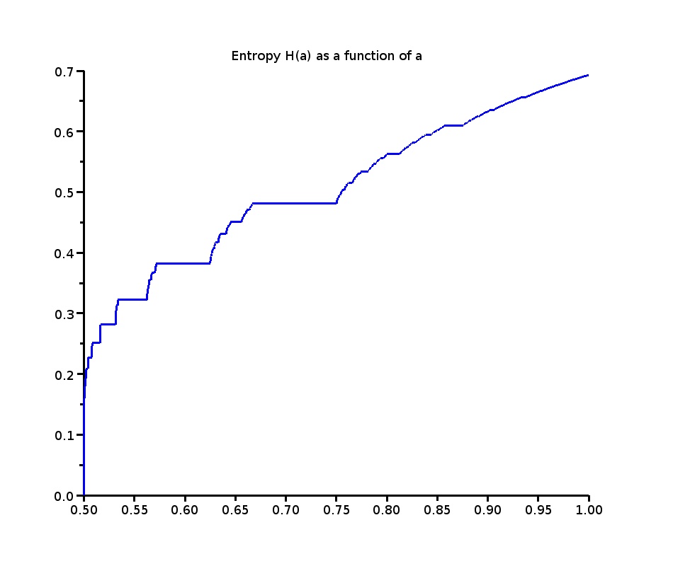
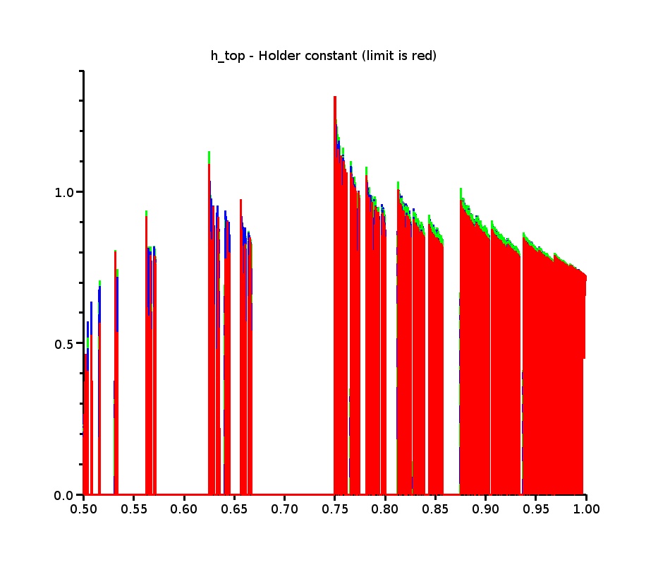
Figure 1. Left: The topological entropy of the doubling map with hole $[a,1]$ as a function of $a$. Right: Estimated local Hölder constant $C(a)$ as a function of $a$ assuming $p=1$ using different mesh-sizes.

In this section we will illustrate and compare Hölder continuity of families of interval maps numerically and theoretically. A non-trivial difficulty in applying our theorems numerically is that an explicit value for the Hölder exponent requires knowledge of the order $p$ of the pole associated with the leading eigenvalue. In our first example below we exhibit a family in which the leading eigenvalue is simple for all parameter values, which in particular implies that $p=1$. We then provide an example exhibiting a double pole and show how this is reflected in numerical experiments.

6.1. Doubling map with left expanding hole

We consider the map $T(x)=2x\mod 1$, defined on $(0,1/2)\cup(1/2,1)$. Let $1/2<a<1$. We will be interested in the topological entropy of $h(a)=h_{\rm top}(T,[a,1])$, that is, $T$ restricted to the set $A=(0,1/2)\cup(1/2,a)$. As shown in the previous section we may calculate this entropy as the leading eigenvalue of a transfer operator. There are essentially two ways to do so. The first is to consider the map $T$ as defined on $I=(0,1/2)\cup(1/2,1)$, and using as weight $g$ the indicator function of $A$. The transfer operator then takes the form

$$(\mathcal{L}_{a}f)(x)=f\left(\frac{x}{2}\right)+\chi_{(0,a)}\left(\frac{1+x}{2}\right)f\left(\frac{1+x}{2}\right)\,.$$

We note that the map has big images as $T^{n}(Z)=(0,1)$ for every $n\in\mathbb{N}$, $Z\in\mathcal{Z}_{n}$. We also have $\Lambda(T)=\Xi(T)=\log 2$. We may apply Theorem 1.2 to see that $h$ is Hölder continuous at every $a\in(1/2,1)$ with the local Hölder exponent satisfying

$${\rm H\ddot{o}l}(h,a)\geq\frac{h(a)}{p\log 2}$$ (29)

for some $p\in\mathbb{N}$. We claim that $p=1$ for each $a\in(1/2,1)$. This is also indicated by numerical experiments illustrated in Figure 1. In that figure we show our numerical estimates of $h(a)=h_{\rm top}(T,[a,1])$ on the left, and on the right the local Hölder constant under the assumption that $p=1$ given by

$$C(a)=\limsup_{s\to a}\frac{|h(s)-h(a)|}{(s-a)^{h(a)/\log 2}}$$

The (numerically obtained) limit superior seems to be neither 0 nor infinity, indicating that our estimate for the local Hölder exponent is optimal.

Now, in order to prove that $p=1$ it suffices to show that the leading eigenvalue is simple. We shall do so by considering an alternative description of the system, using a Hofbauer tower ([Hof], see also [BaK, Section 3]), which we also used to compute our numerical estimates.

We start out by writing $J_{0}=(0,1/2)$, $J_{1}=(1/2,a)$, and $J_{2}=(a,1)$. Set ${\mathcal{Z}}=\{J_{0},J_{1},J_{2}\}$ and consider the locally constant weight $g=\chi_{J_{1}\cup J_{2}}$. For simplicity of notation we shall in the following tacitly omit intervals arising from $J_{2}$ from the Hofbauer tower as they will not contribute to the spectral properties of the transfer operator on the tower.

Instead of working with cylinder sets, that is, intersections of preimages of the $J_{i}$’s, the idea is to deal with intersections of forward iterates of these intervals. In our case, this boils down to studying the forward orbit of the point $a$. To this end, we define the sequence $(a_{n})_{n\geq 0}$ by setting $a_{0}=a$ and $a_{k+1}=T(\min\{a,a_{k}\}^{-})\in[0,a_{1}]$ for $k\geq 0$, where $T(x^{-})=\lim_{\xi\uparrow x}T(\xi)$ for $x\in(0,1]$.

The sequence contains finitely many values if either $a_{k}\geq a$ for some $k$, which happens when the orbit of $a$ ‘escapes’, or if $a$ is pre-periodic for $T$. Otherwise the orbit is infinite.

Let us first consider the case when the orbit is infinite, so in particular we have $0<a_{k}<a$ and $a_{k}\neq 1/2$ for all $k\geq 1$. We set ${\mathcal{D}}_{0}=T(J_{0})=(0,1)$ and define the ‘flats’ ${\mathcal{D}}_{k}=(0,a_{k})$ for $k\geq 1$. We have the following ‘transition’ rules giving rise to a transition matrix $M$ (elements other than those mentioned all being zero):

$$\begin{array}[]{lcllll}\ 0<a_{k}<1/2&:&{\mathcal{D}}_{k+1}&=T({\mathcal{D}}_{k}\cap J_{0})&=(0,a_{k+1}),&M_{k,k+1}=1,\\ \ 1/2<a_{k}<1&:&{\mathcal{D}}_{k+1}&=T({\mathcal{D}}_{k}\cap J_{1})&=(0,a_{k+1}),&M_{k,k+1}=1,\\ \ 1/2\leq a_{k}<1&:&{\mathcal{D}}_{0}&=T({\mathcal{D}}_{k}\cap J_{0})&=(0,1),&M_{k,0}=1.\\ \end{array}$$

Note that the above lines describe two cases: if $a_{k}<1/2$, then there is exactly one transition, namely from ${\mathcal{D}}_{k}$ to ${\mathcal{D}}_{k+1}$; if $a_{k}>1/2$, then two different transitions are possible, namely the one from ${\mathcal{D}}_{k}$ to ${\mathcal{D}}_{k+1}$ and an additional one from ${\mathcal{D}}_{k}$ to the bottom flat ${\mathcal{D}}_{0}$.

For later use, let $A=\left\{\,{k\geq 0}\,:\,{a_{k}\geq 1/2}\,\right\}$ denote the set of indices for which there is a transition from the $k$-th flat to the bottom flat. Note that $0\in A$ and that $A$ contains at least one more index, the latter being a consequence of the fact that $T$ is expanding.

The Hofbauer tower is now defined as the disjoint union of flats

$$\widehat{\mathcal{D}}=\left\{\,{(x,{\mathcal{D}}_{k})}\,:\,{k\geq 0,\ x\in{\mathcal{D}}_{k}}\,\right\}\,.$$

With the tower we associate a directed graph ${\mathcal{G}}$ obtained from the transition matrix. A possible transition graph is sketched in Figure 2.

Figure 2. The transition graph ${\mathcal{G}}$ in the case of $A=\{0,2,4,\ldots\}$

By [BaK, Theorem 2 and Lemma 4.1], the multiplicity of the leading eigenvalue $\lambda$ of the transfer operator $\mathcal{L}_{a}$ equals the order of the leading pole $z=1/\lambda$ of the zeta-function associated with the tower, which is given by

$$\zeta(z)=\exp\sum_{k=1}^{\infty}\widehat{\zeta}_{k}\frac{z^{k}}{k}\,,$$

where $\widehat{\zeta}_{k}$ is the total number of periodic points in ${\mathcal{G}}$ of period $k$ (not necessarily prime).

Now, by Hofbauer [Hof, Theorem 1 as well as Lemmas 3 and 4] this periodic orbit counting zeta-function has the same poles in the unit disk as the zeros of a determinant calculated in the following way: call $\gamma=(i_{0}i_{1}\cdots i_{n-1})$ a simple cycle if $M_{i_{0}i_{1}}\cdots M_{i_{n-1}i_{0}}=1$ and all the $i$’s are distinct. Also denote by $|\gamma|=n$ the length of such a cycle. Then

$$d(z)=1+\sum\left(-z^{|\gamma_{1}|}\right)\cdots\left(-z^{|\gamma_{q}|}\right)$$ (30)

where the sum is over all $q$-tuples (with $q\geq 1$) of disjoint simple cycles of ${\mathcal{G}}$.

When a transition matrix $M$ is of finite size $N\times N$ the formula follows easily from the standard expansion of $d(z)=\det(I-zM)$ in terms of permutations and rewriting permutations as products over distinct cycles. In the case of unbounded matrix size we refer to [Hof] which explains how to take a limit of finite matrix truncations, that is, levels in the Hofbauer tower. Combining the above two results we have:

Theorem 6.1.

Let $z\in\mathbb{C}$ with $0<\left|{z}\right|<1$. Then $z$ is a zero of $d$ iff $1/z$ is an eigenvalue of the transfer operator. Moreover, if this is the case the order of the zero equals the (algebraic) multiplicity of the eigenvalue.

In order to apply the theorem above to the present situation we requite a simple lemma on the nature of the zeros closest to the origin of certain power series.

Lemma 6.2.

Let $(m_{k})_{k\geq 1}$ denote a sequence with $m_{k}\in{\{0,1\}}$ such that $m_{k}=1$ for at least one $k\geq 1$. Then

$$\delta(z)=1-z-\sum_{k=1}^{\infty}m_{k}z^{k+1}$$

is holomorphic in the open unit disk. Moreover, there is a unique $r\in(0,1)$ which is a simple zero of $\delta$ and all other zeros of $\delta$ are strictly larger in modulus.

Proof.

By the Cauchy-Hadamard Theorem, the function $\delta$ is holomorphic in the open unit disk. Furthermore, we have $|\delta(z)|\geq 1-\left|{z}\right|-\sum_{k=1}^{\infty}m_{k}|z|^{k+1}=\delta(|z|)$ with equality iff $z$ is real and positive. Since $\delta(0)=1$ and $\delta(z)<0$ for $z$ real and sufficiently close to $1$ there is $r\in(0,1)$ with $d(r)=0$. Moreover, since $|\delta(\lambda)|>\delta(|\lambda|)$ when $\lambda\notin[0,1)$, any other zero must be of absolute value strictly larger than $r$, and noting that $d^{\prime}(r)=-1-\sum_{k=1}^{\infty}(k+1)m_{k}r^{k}<0$ the order of the zero must be one. ∎

Returning to our specific case when the orbit of $a$ is infinite we obtain the following.

Proposition 6.3.

Suppose that the orbit $(a_{k})_{k\geq 0}$ is infinite. Then the Hofbauer determinant (30) is given by

$$d(z)=1-\sum_{k=0}^{\infty}M_{k,0}\,z^{k+1}$$

and is holomorphic in the open unit disk. There is a unique $r\in(0,1)$ which is a simple zero of $d$ and all other zeros of $d$ are of strictly larger modulus. The spectral radius of the transfer operator equals $1/r$ and is a simple eigenvalue. All other spectral values are strictly smaller in modulus than $1/r$.

Proof.

Cycles are to be distinct in the above sum and any cycle in our transition graph has to contain ${\mathcal{D}}_{0}$ so there are no two distinct non-trivial cycles. Since every cycle is of the form $({\mathcal{D}}_{0}{\mathcal{D}}_{1}\cdots{\mathcal{D}}_{k})$ with $M_{k,0}=1$ we immediately obtain the expression for the Hofbauer determinant.

The remaining assertions now follow from Theorem 6.1 and Lemma 6.2 by observing that $d(z)=1-\sum_{k\in A}^{\infty}z^{k+1}$, that $0\in A$ and that $A\setminus{\{0\}}$ is non-empty. ∎

We now turn to the case where the Hofbauer tower is finite. Recall that this happens precisely if $a$ is pre-periodic for $T$ or if the orbit escapes. In either case there are $N$ and $1\leq j\leq N$ with $a_{N+1}=a_{j}$; note that if the orbit escapes we have $a_{N+1}=a_{1}$. Thus there is no element $M_{N,N+1}$ but we have the additional transition $M_{N,j}=1$.

We then have the following simple cycles:

1. For $0\leq k\leq N$ with $M_{k,0}=1$, $({\mathcal{D}}_{0}{\mathcal{D}}_{1}\cdots{\mathcal{D}}_{k})$ is of length $k+1$.

2. One additional cycle of the form $({\mathcal{D}}_{j}\cdots{\mathcal{D}}_{N})$ and of length $N-j+1$.

In this case there is also the possibility of disjoint $2$-tuples for each $0\leq k<j$ with $M_{0,k}=1$ of the form

$$\{({\mathcal{D}}_{0}{\mathcal{D}}_{1}\cdots{\mathcal{D}}_{k}),({\mathcal{D}}_{j}\cdots{\mathcal{D}}_{N})\}.$$ (31)

The Hofbauer determinant (30) then takes the form

$$d(z)= 1-z^{N-j+1}-\sum_{k=0}^{N}M_{k,0}\,z^{k+1}+\sum_{k=0}^{j-1}M_{k,0}\,z^{k+1}z^{N-j+1}$$

$$= \left(1-z^{N-j+1}\right)\left(1-\sum_{k=0}^{j-1}M_{k,0}\,z^{k+1}-\left(1-z^{N-j+1}\right)^{-1}\sum_{k=j}^{N}M_{k,0}\,z^{k+1}\right)$$

$$= \left(1-z^{N-j+1}\right)\left(1-\sum_{k=0}^{\infty}\widetilde{M}_{k,0}\,z^{k+1}\right)$$

where

$$\widetilde{M}_{k,0}=\begin{cases}M_{k,0}&\text{for $0\leq k<j$,}\\ M_{j+(k-j\mod(N-j+1)),0}&\text{for $k\geq j$.}\end{cases}$$ (32)

We may thus conclude:

Proposition 6.4.

Suppose that the orbit $(a_{k})_{k\geq 0}$ is finite. Then the Hofbauer determinant (30) is given by

$$d(z)=\left(1-z^{N-j+1}\right)\left(1-\sum_{k=0}^{\infty}\widetilde{M}_{k,0}z^{k+1}\right)$$

for some $N$ and $j$ with $1\leq j\leq N$ and $\widetilde{M}_{k,0}$ gven by (32). The function $d$ is holomorphic in the open unit disk. Moreover, there is a unique $r\in(0,1)$ which is a simple zero of $d$ and all other zeros of $d$ are of strictly larger modulus. The spectral radius of the transfer operator equals $1/r$ and is a simple eigenvalue. All other spectral values are strictly smaller in modulus than $1/r$.

Proof.

This follows from the calculation above together with Theorem 6.1 and Lemma 6.2. ∎

Summarising, we have shown the following.

Corollary 6.5.

For any $a\in(1/2,1)$ the transfer operator $\mathcal{L}_{a}$ has a leading eigenvalue which is simple. In particular, the topological entropy $h(a)$ of the doubling map with hole $[a,1]$ satisfies

$${\rm H\ddot{o}l}(h,a)\geq\frac{h(a)}{\log 2}\,.$$

6.2. Doubling map with hole giving rise to a double pole

One of the dynamically simplest examples exhibiting a double pole of the resolvent is again furnished by the doubling map $T(x)=2x\mod 1$. This time, however, we introduce a hole from $a$ to $a+1/12$, that is, we shall consider $h_{\rm top}(T,[a,a+1/12])$ as a function of $a$. For the particular value $a=3/4$ the hole is from $3/4$ to $5/6$. Figure 3 shows this map indicating orbits of boundary points.

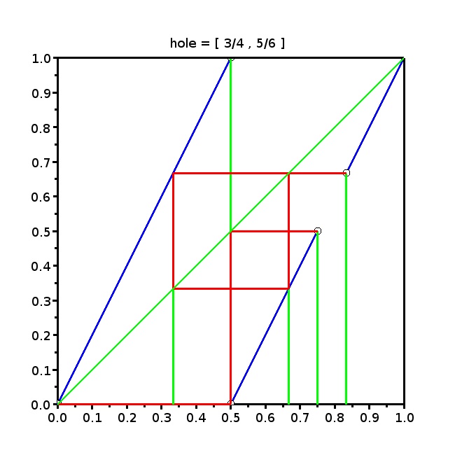
Figure 3. The doubling map with hole $[3/4,5/6]$ showing orbits of the hole boundaries.

The estimated entropy $h_{\rm top}(T,[a,a+1/12])$ as a function of $a$ is shown in Figure 5 on the left, exhibiting a ‘dip’ at $a=3/4$. In order to understand this dip, note that the intervals $I_{1}=(0,1/2)$, $I_{2}=(1/2,3/4)$, and $I_{3}=(5/6,1)$ make up the initial partition. Introducing $I_{4}=(2/3,3/4)$ and $I_{5}=(1/3,1/2)$ we have the following transitions (see Figure 4 for the corresponding transition graph):

$$\text{\raisebox{0.5pt}{\raisebox{-.9pt} {1}⃝}}\to\text{\text{\raisebox{0.5pt}{\raisebox{-.9pt} {1}⃝}}, \text{\raisebox{0.5pt}{\raisebox{-.9pt} {2}⃝}} or \text{\raisebox{0.5pt}{\raisebox{-.9pt} {3}⃝}}}\,;\quad\text{\raisebox{0.5pt}{\raisebox{-.9pt} {2}⃝}}\to\text{\raisebox{0.5pt}{\raisebox{-.9pt} {1}⃝}}\,;\quad\text{\raisebox{0.5pt}{\raisebox{-.9pt} {3}⃝}}\to\text{\text{\raisebox{0.5pt}{\raisebox{-.9pt} {3}⃝}} or \text{\raisebox{0.5pt}{\raisebox{-.9pt} {4}⃝}}}\,;\quad\text{\raisebox{0.5pt}{\raisebox{-.9pt} {4}⃝}}\to\text{\raisebox{0.5pt}{\raisebox{-.9pt} {5}⃝}}\,;\quad\text{\raisebox{0.5pt}{\raisebox{-.9pt} {5}⃝}}\to\text{\text{\raisebox{0.5pt}{\raisebox{-.9pt} {3}⃝}} or \text{\raisebox{0.5pt}{\raisebox{-.9pt} {4}⃝}}}\,.$$

Figure 4. The transition graph ${\mathcal{G}}$ in the double pole case

One verifies that $\gamma=(1+\sqrt{5})/2$ is a double eigenvalue of the corresponding transition matrix $\pi$ (see Figure 5 right) and that $\ker(\pi-\gamma I)$ is one-dimensional. This implies that the resolvent has a double pole at $\gamma$. Theorem 1.2 applied at $a=3/4$ shows that the entropy $h(a)=h_{\rm top}(T,[a,a+1/12])$ is Hölder continuous with a local exponent at least $\log(\gamma)/(2\log 2)\approx 0.3471$ which is consistent with a numerical estimate for the exponent (not shown).

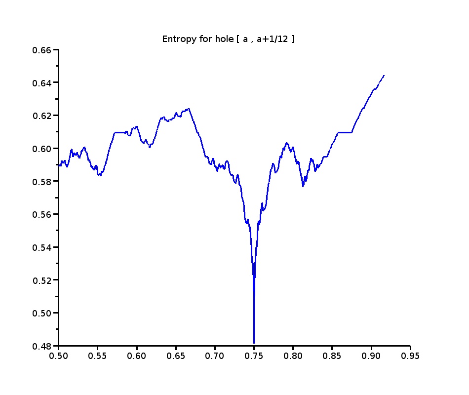
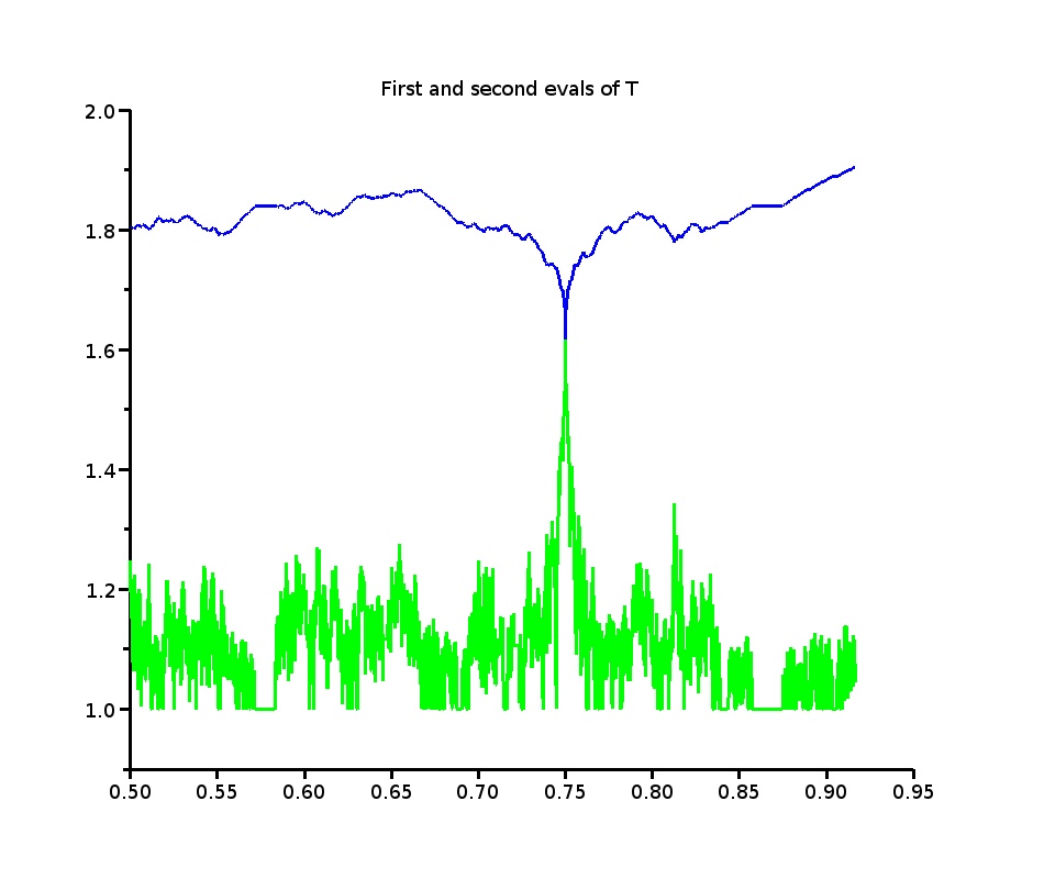
Figure 5. Left: the topological $h_{\rm top}(T,[a,a+1/12])$ as a function of $a$. Note the dip for $a=3/4$. Right: the two largest eigenvalues of the transfer operator.

References

- [BBF] W. Bahsoun, C. Bose and G. Froyland (eds). Ergodic Theory, Open Dynamics, and Coherent Structures. New York, Springer, 2014.
- [BaK] V. Baladi and G. Keller. Zeta functions and transfer operators for piecewise monotone transformations. Commun. Math. Phys. 127 (1990) 459–477.
- [BeC] H. van den Bedem and N. Chernov. Expanding maps of an interval with holes. Ergodic Theory Dynam. Systems 22 (2002) 637–654.
- [BoG] A. Boyarsky and P. Gora. Laws of Chaos: Invariant Measures and Dynamical Systems in One Dimension. Boston, Birkhäuser, 1997.
- [BrDM] H. Bruin, M. Demers and I. Melbourne. Existence and convergence properties of physical measures for certain dynamical systems with holes. Ergod. Th. & Dynam. Sys. 30 (2010) 687–728.
- [BY] L. Bunimovich and A. Yurchenko. Where to place a hole to achieve a maximal escape rate. Israel J. Math. 182 (2008) 229-252.
- [CaT] C. Carminati and G. Tiozzo. The local Hölder exponent for the dimension of invariant subsets of the circle. Ergod. Th. & Dynam. Sys., doi:10.1017/etds.2015.135, in press.
- [Cha] F. Chatelin. Spectral Approximation of Linear Operators. New York, Academic Press, 1983.
- [CMa] N. Chernov and R. Markarian. Ergodic properties of Anosov maps with rectangular holes. Bol. Soc. Brasil. Mat. 28 (1997) 271–314.
- [CMaT] N. Chernov, R. Markarian and S. Troubetzkoy. Conditionally invariant measures for Anosov maps with small holes. Ergodic Theory Dynam. Systems 18 (1998) 1049–1073.
- [CMS] P. Collet, S. Martínez and B. Schmitt. The Yorke-Pianigiani measure and the asymptotic law on the limit Cantor set of expanding systems. Nonlinearity 7 (1994) 1437–1443.
- [CrKD] G. Cristadoro, G. Knight and M. Degli Esposti. Follow the fugitive: an application of the method of images to open systems. J. Phys. A 46 (2013) 272001, 8 pp.
- [DemW] M. Demers and P. Wright. Behaviour of the escape rate function in hyperbolic dynamical systems. Nonlinearity 25 (2012) 2133–2150.
- [DemWY] M. Demers, P. Wright and L-S. Young. Escape rates and physically relevant measures for billiards with small holes. Comm. Math. Phys. 294 (2010) 353–388.
- [Det] C. Dettmann. Open circle maps: small hole asymptotics. Nonlinearity 26 (2013) 307–317.
- [DS] N. Dunford and J. T. Schwartz. Linear Operators. Part I. General Theory. New York, Interscience, 1958.
- [FP] A. Ferguson and M. Pollicott. Escape rates for Gibbs measures. Ergod. Th. & Dynam. Sys. 32 (2012) 961–988.
- [G] E. Giusti. Minimal Surfaces and Functions of Bounded Variation. Boston, Birkhäuser, 1984.
- [Gu] J. Guckenheimer. The growth of topological entropy for one-dimensional maps. In Z. Nitecki and C. Robinson, Global theory of dynamical systems (Proc. Internat. Conf., Northwestern Univ., Evanston, Ill., 1979), Lecture Notes in Mathematics 819, Berlin, Springer, 1980, pp. 216–223.
- [Hen] H. Hennion. Sur un théorème spectral et son application aux noyaux lipchitziens. Proc. Amer. Math. Soc. 118 (1993) 627–634.
- [Hof] F. Hofbauer. Periodic points for piecewise monotonic transformations. Ergod. Th. & Dynam. Sys. 5 (1985) 237–256.
- [HoK] F. Hofbauer and G. Keller. Ergodic properties of invariant measures for piecewise monotonic transformations. Math. Z. 180 (1982) 119–140.
- [IM] C.T. Ionescu Tulcea and G. Marinescu. Théorie ergodique pour des classes d’opérations non complètement continues. Ann. of Math. 52 (1950) 140–147.
- [IP] S. Isola and A. Politi. Universal encoding for unimodal maps. J. Statist. Phys. 61 (1990) 263–291.
- [Kat] T. Kato. Perturbation Theory for Linear Operators. 2nd edition, Berlin, Springer-Verlag, 1980.
- [Ke] G. Keller. On the rate of convergence to equilibrium in one-dimensional systems. Commun. Math. Phys. 96 (1984) 181–193.
- [KeL1] G. Keller and C. Liverani. Stability of the spectrum for transfer operators. Ann. Scuola Norm. Sup. Pisa Cl. Sci. (4) 28 (1999) 141–152.
- [KeL2] G. Keller and C. Liverani. Rare events, escape rates and quasistationarity: some exact formulae. J. Stat. Phys. 135 (2009) 519–534.
- [LM] C. Liverani and V. Maume-Deschamps. Lasota-Yorke maps with holes: conditionally invariant probability measures and invariant probability measures on the survivor set. Ann. Inst. H. Poincaré Probab. Statist. 39 (2003) 385–412.
- [MS] M. Misiurewicz and W. Szlenk. Entropy of piecewise monotone mappings. Studia Math. 67 (1980) 45–63.
- [PY] G. Pianigiani and J.A. Yorke. Expanding maps on sets which are almost invariant. Decay and chaos. Trans. Amer. Math. Soc. 252 (1979) 351–366.
- [R] H.H. Rugh. Intermittency and regularized Fredholm determinants. Inv. Math. 135 (1999) 1–24.
- [Ryc] M. Rychlik. Bounded variation and invariant measures. Studia Math. 76 (1983), 69–80.
- [S] H.H. Schaefer. Topological Vector Spaces, 2nd ed., with M. P. Wolff. New York, Springer, 1999.
- [U] M. Urbański. On Hausdorff dimension of invariant sets for expanding maps of a circle. Ergod. Th. & Dynam. Sys. 6 (1986) 295–309.