Polarization microlensing in the quadruply imaged broad absorption line quasar H1413+117

We have obtained spectropolarimetric observations of the four images of the gravitationally lensed broad absorption line quasar H1413+117. The polarization of the microlensed image D is significantly different, both in the continuum and in the broad lines, from the polarization of image A, which is essentially unaffected by microlensing. The observations suggest that the continuum is scattered off two regions, spatially separated, and producing roughly perpendicular polarizations. These results are compatible with a model in which the microlensed polarized continuum comes from a compact region located in the equatorial plane close to the accretion disk and the non-microlensed continuum from an extended region located along the polar axis.

1 Introduction

Spectropolarimetry is a powerful tool to study and disentangle the inner regions of quasars, otherwise impossible to resolve spatially. Most often optical linear polarization originates from scattering off a separate region that acts as a mirror. In this kind of situation, the separation of the polarized light from the unpolarized light usually offers an additional line of sight to different quasar regions, providing information about the geometry and location of quasar components, such as the source of continuum or the broad emission/absorption line regions (e.g., Antonucci and Miller ant85 (1985); Smith et al. smi04 (2004); Kishimito et al. kis08 (2008)).

Gravitational microlensing, on the other hand, can selectively magnify quasar inner regions, such as the accretion disk or even part of the broad line region, in one of the lensed images. A comparison with unaffected images can provide constraints on the size, location, and kinematics of the quasar inner regions (e.g., Eigenbrod et al. eig08 (2008); Blackburne et al. bla11 (2011); Sluse et al. slu11 (2011); Braibant et al. bra14 (2014)).

Broad absorption lines (BALs) are seen in approximately 20% of optically selected quasars (Knigge et al. kni08 (2008)). BAL quasars are characterized by deep blueshifted absorption in the resonance lines of ionized species revealing fast and massive outflows, which likely affect the evolution of the host galaxy and intergalactic medium (Silk and Rees sil98 (1998)). Spectropolarimetry has proved useful to constrain the geometry and dynamics of the outflows, which are usually attributed to roughly equatorial winds launched from the accretion disk (Goodrich and Miller goo95 (1995); Ogle et al. ogl99 (1999); Lamy and Hutsemékers lam04 (2004); Young et al. you07 (2007)), although polar winds are observed in some radio-loud BAL quasars (Zhou et al. zho06 (2006); Ghosh and Punsly gho07 (2007); DiPompeo et al. dip13 (2013); Bruni et al. bru13 (2013)). In one particular case, microlensing has helped to disentangle the intrinsic absorption line from the emission line profile, providing evidence for outflows with both equatorial and polar components. (Hutsemékers et al. hut10 (2010), hereafter Paper I).

Here, we report on the first spectropolarimetric observations of the four images of a gravitationally lensed quasar, the quadruply imaged broad absorption line quasar H1413+117, known to be both polarized and microlensed (Angonin et al. ang90 (1990); Hutsemékers hut93 (1993); Østensen et al. ost97 (1997); Chae et al. cha01 (2001); Anguita et al. ang08 (2008); Paper I; O’Dowd et al. odo15 (2015)). In Sluse et al. (slu15 (2015), hereafter Paper II), we have unveiled the existence of two sources of continuum, especially a spatially separated or extended continuum source, using differences induced by microlensing in the total flux spectra. The present paper focuses on the analysis of the polarization of the individual images. Broadband polarization measurements of the four images were already reported in Chae et al. (cha01 (2001)) and in Paper I, with inconclusive results (see also Hales and Lewis hal07 (2007)).

2 Observations and data reduction

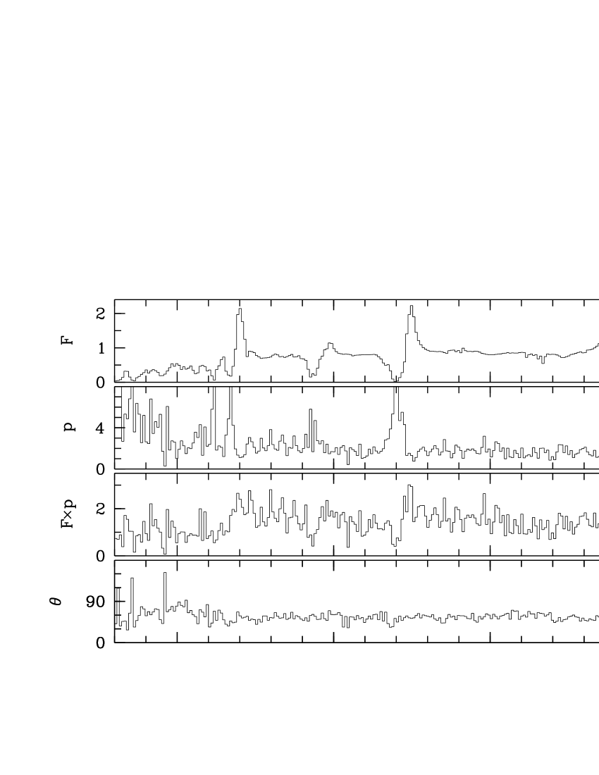
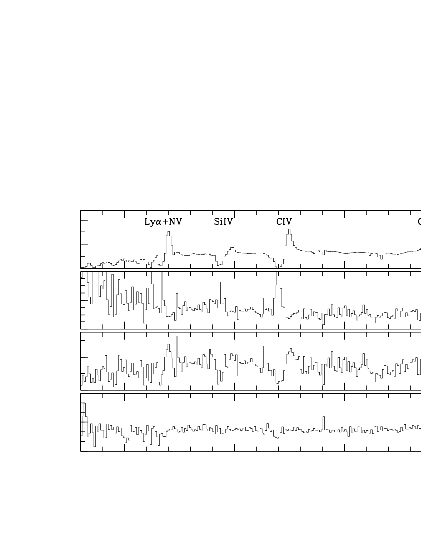
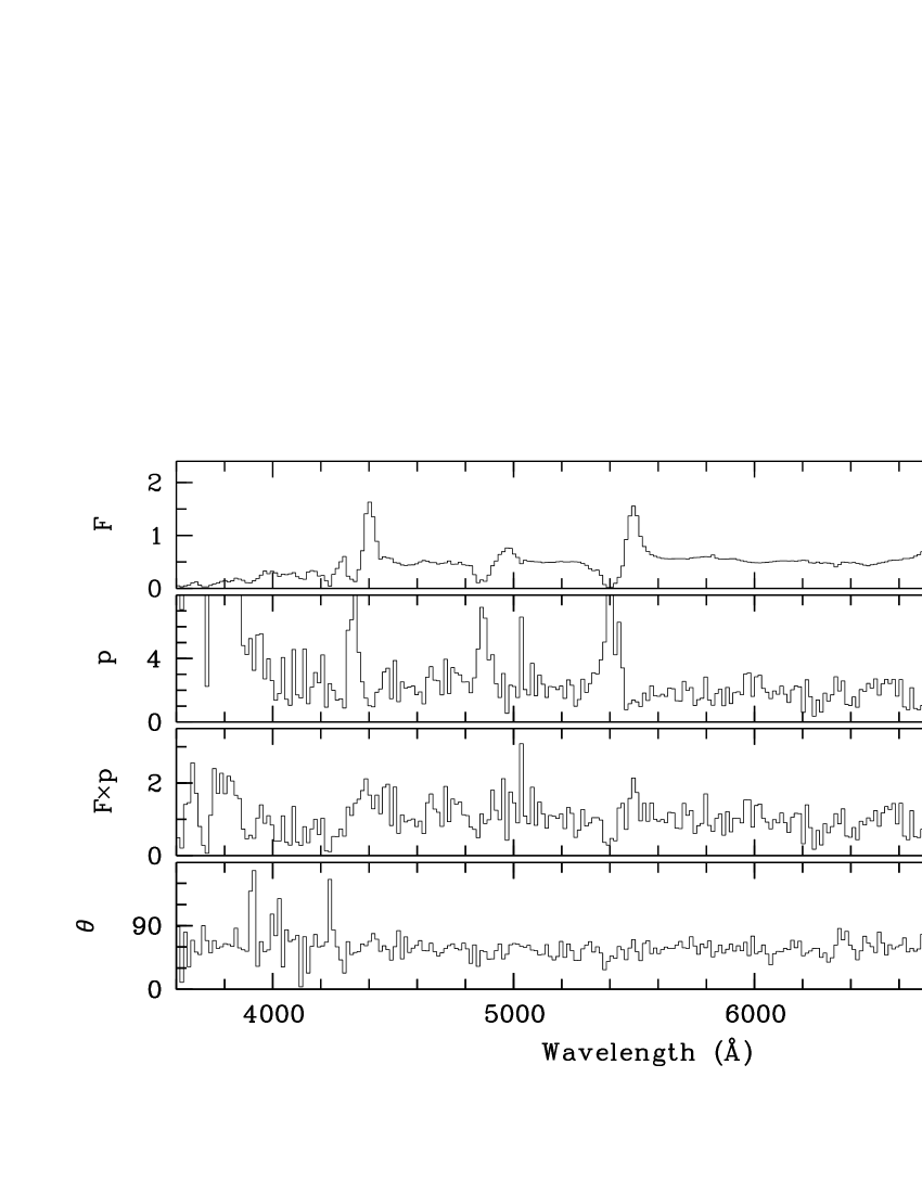
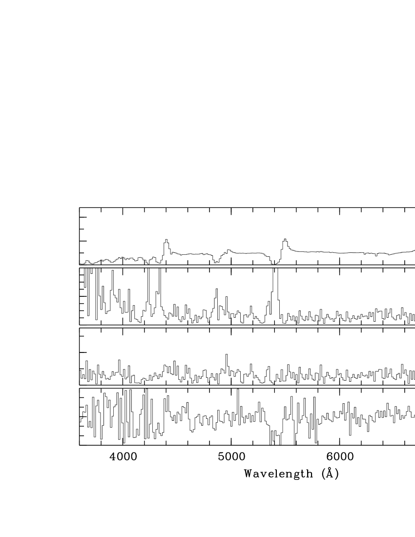
Figure 1: The total flux $F(\lambda)$, (in arbitrary units), the linear polarization degree $p(\lambda)$, (in %), the polarized flux $F(\lambda)\times p(\lambda)$, (in arbitrary units), and the polarization position angle $\theta(\lambda)$, (in degree, east of north) for images A, B, C, D of H1413+117.

The observations were carried out in March-April 2011 with the ESO Very Large Telescope equipped with the FORS2 instrument in its linear spectropolarimetry mode (FORS User Manual, VLT-MAN-ESO-13100-1543). The spectra were obtained by positioning a 0$\aas@@fstack{\prime\prime}$4-wide MOS slit through either the A-D or the B-C images of H1413+117 (naming convention from Paper I). Grisms 300V and 300I were used to cover the 0.36-0.90 $\mu$m and 0.60-1.03 $\mu$m spectral ranges, respectively. Each observation was carried out twice with a seeing better than 0$\aas@@fstack{\prime\prime}$6 (cf. Paper II, for other details). Exposures of 660s each were secured with the half-wave plate rotated at the position angles 0°, 22.5°, 45°, and 67.5°. For each image and grism, 16 spectra (two orthogonal polarizations, four half-wave plate angles, two epochs) were obtained and extracted by fitting Moffat profiles along the slit.

For each image of H1413+117, the normalized Stokes parameters $q(\lambda)$ and $u(\lambda)$, the linear polarization degree $p(\lambda)$, the polarization position angle $\theta(\lambda)$, the total flux $F(\lambda)$, and the polarized flux $F(\lambda)\times p(\lambda)$ were computed from the individual spectra according to standard recipes (e.g., FORS manual). To increase the signal to noise ratio, the original spectra were rebinned over 15Å wavelength ($\sim$9 pixel) bins and the two epochs added before computing the polarimetric data. The spectra were corrected for the retarder plate zero angle given in the FORS manual. The final blue spectra are illustrated in Fig. 1. Contamination by interstellar polarization in our Galaxy is negligible for H1413+117 (Hutsemékers et al. hut98 (1998); Ogle et al. ogl99 (1999)).

To enable comparison with previous broadband polarization measurements, we integrated the spectra over the FORS2 V High filter and measured the broadband polarizations reported in Table 1. The quoted uncertainties are estimated from the differences between the measurements obtained at the two epochs (separated by at most 26 days), which are in excellent agreement. Since the C iv line appears in the V filter, we also measured the polarization by integrating over a continuum region excluding C iv, namely the 0.57-0.64 $\mu$m wavelength range. The difference between these two sets of broadband measurements is negligible. Finally, polarization integrated over the FORS2 I Bessel filter is also given, using both the 300V and 300I data sets.

3 The polarization of the four images

3.1 Overview

The broadband measurements confirm the variability in both degree and angle of the polarization in H1413+117, which was first reported by Goodrich and Miller (goo95 (1995)).

In 2011, there was a net decrease of the continuum polarization degree of image D with respect to the other images and previous epochs (Table 1). The polarization angle measured for image D also appears significantly different, by $\sim$25°, from the angles measured in the other images. This difference is roughly constant with time, apparently superimposed on intrinsic variations that affect all images.

In agreement with previous spectropolarimetric observations (Goodrich and Miller goo95 (1995); Ogle et al. ogl99 (1999); Lamy and Hutsemékers lam04 (2004)), we find a strong increase of the polarization degree in the BAL troughs. The strongest, low-velocity absorption component is present but shallower in polarized flux than in total flux. These polarization properties are usually interpreted by electron or dust scattering of the continuum, where the scattered light is less absorbed than the direct light.

For images A, B, and C, a small rotation of the polarization angle is observed in the BAL troughs, in particular C iv, suggesting the presence of two polarization sources with different polarization angles. The N v, the C iv, and possibly the Si iv emission lines appear in the polarized flux, but they are less polarized than the continuum. Although the polarization data of image D are noisier, the C iv absorption line is seen in the polarized flux with no significant emission line. In that image, a strong rotation of the polarization angle is observed across a large part of the C iv line profile.

3.2 The continuum polarization: Analysis of the (D,A) pair

We focus on the (D,A) pair of images because at rest-frame optical-UV wavelengths, image D is strongly microlensed while only image A is not (Paper II). The fact that the polarization angle of the continuum of image D is rotated with respect to the polarization angle of the continuum of image A requires two sources of polarized continuum with different polarization angles, one which is microlensed and the other not. Because its magnification decreases with increasing wavelength, the microlensed continuum source was identified in Paper II as the accretion disk. This microlensed polarized continuum then originates from a compact source, presumably disk-like, close to the accretion disk or from the accretion disk itself.

Table 1: Broadband polarization of the four images of H1413+117

Epoch / Band	A	B	C	D
		$p\;(\%)$
1999 / F555W	1.6$\pm$0.5	2.3$\pm$0.5	1.8$\pm$0.5	2.9$\pm$0.5
2008 / V	1.4$\pm$0.1	2.4$\pm$0.1	1.2$\pm$0.1	2.0$\pm$0.1
2011 / V	1.7$\pm$0.1	2.2$\pm$0.1	1.9$\pm$0.1	0.7$\pm$0.1
2011 / Vc	1.7$\pm$0.1	2.0$\pm$0.1	1.7$\pm$0.1	0.8$\pm$0.2
2011 / I	1.7$\pm$0.3	1.7$\pm$0.3	1.5$\pm$0.2	1.0$\pm$0.2
		$\theta\;(\degr)$
1999 / F555W	75$\pm$9	65$\pm$6	71$\pm$8	102$\pm$5
2008 / V	72$\pm$2	79$\pm$1	69$\pm$3	96$\pm$2
2011 / V	55$\pm$2	65$\pm$2	57$\pm$2	82$\pm$4
2011 / Vc	56$\pm$2	63$\pm$2	57$\pm$2	86$\pm$8
2011 / I	47$\pm$5	64$\pm$5	55$\pm$4	78$\pm$6

The linear polarization degree $p$ is given in percent and the polarization position angle $\theta$ in degree, east of north. The data obtained in 2008 and 1999 are from Paper I and from Chae et al. (cha01 (2001)), respectively. For the 2011 data, V and I refer to measurements integrated over the FORS2 V and I filters, and Vc over the 0.57 - 0.64 $\mu$m wavelength range.

Under the hypothesis that the observed continuum polarization is the sum of the polarization from a microlensed compact source and a non-microlensed extended one, we can extract the intrinsic polarizations of the two sources, $p_{c}$, $\theta_{c}$, $p_{e}$, $\theta_{e}$, as detailed in Appendix A. The results are listed in Table 2. They were derived from the broadband measurements using the magnification factor $\mu$ =2.0 assumed constant with time (Paper II). Three values of $F_{e}/F_{c}$, the flux ratio between the extended and compact continua, are considered.

Although differences exist, likely due to the oversimplified model considered here, the results appear remarkably consistent for the different epochs and wavelength bands. The polarization of the compact source is around $p_{c}\sim 3\%$ and $\theta_{c}\sim 115\degr$. The polarization of the extended source is around $p_{e}\sim 10\%$ and $\theta_{e}\sim 35\degr$. The polarizations appear roughly orthogonal. They can be produced by electron or dust scattering (Brown and McLean bro77 (1977); Goosmann and Gaskell goo07 (2007)). These results are consistent with a single central source of continuum, the accretion disk, which is scattered off a compact low-polarization region close to it in the equatorial plane and a separated, extended, high-polarization region located along the accretion disk axis, i.e., in a polar region. The whole system is observed at intermediate- to high-inclination (Ogle ogl97 (1997); Lamy and Hutsemékers lam04 (2004); Smith et al. smi04 (2004)). The model is schematically illustrated in Fig. 2.

These results depend little on the exact values of $\mu$ (which may be lower at the I band wavelength) and of $F_{e}/F_{c}$. A significant ($\gtrsim$ 0.2) contribution from the non-microlensed continuum is nevertheless required to keep the polarization $p_{e}$ at reasonable levels and to avoid fine-tuning, in agreement with the results of Paper II. These values of $F_{e}/F_{c}$ are compatible with the fraction of polar scattered flux computed from models (e.g., Brown and McLean bro77 (1977); Goosmann and Gaskell goo07 (2007)).

Time variability can be due to changes of the polarization or to a variation of the $F_{e}/F_{c}$ ratio. Interestingly, with $p_{c}$, $\theta_{c}$, $p_{e}$, $\theta_{e}$ fixed, adopting a higher $F_{e}/F_{c}$ ratio in 2011 than at previous epochs, as suggested in Paper II, rotates all polarization angles toward $\theta_{e}$ and decreases the polarization degree in image D, in (qualitative) agreement with the observations (Table 1).

Table 2: Results from the polarization model applied to the (D,A) pair

Epoch / Band	$F_{e}/F_{c}$	$p_{c}\;(\%)$	$\theta_{c}\;(\degr)$	$p_{e}\;(\%)$	$\theta_{e}\;(\degr)$
1999 / F555W	0.2	5.6$\pm$2.2	111$\pm$11	27.3$\pm$15.	32$\pm$16
	0.5	6.3$\pm$2.3	112$\pm$12	12.5$\pm$7.3	34$\pm$17
	0.8	7.1$\pm$3.0	113$\pm$12	8.9$\pm$5.3	35$\pm$17
2008 / V	0.2	3.5$\pm$0.5	107$\pm$4	16.6$\pm$3.2	31$\pm$6
	0.5	3.9$\pm$0.6	108$\pm$4	7.7$\pm$1.5	34$\pm$6
	0.8	4.3$\pm$0.6	109$\pm$4	5.5$\pm$1.1	36$\pm$6
2011 / V	0.2	1.7$\pm$0.4	121$\pm$8	16.9$\pm$3.0	44$\pm$5
	0.5	2.0$\pm$0.5	124$\pm$7	8.6$\pm$1.4	46$\pm$5
	0.8	2.4$\pm$0.6	125$\pm$7	6.5$\pm$1.1	46$\pm$5
2011 / I	0.2	2.1$\pm$1.0	105$\pm$13	17.4$\pm$6.9	31$\pm$11
	0.5	2.5$\pm$1.2	107$\pm$13	8.7$\pm$3.3	32$\pm$11
	0.8	2.9$\pm$1.3	109$\pm$13	6.5$\pm$2.4	33$\pm$11

3.3 The polarization in the line profiles

The increase of the polarization degree in the BAL troughs and the presence of shallower BALs in the polarized flux (Fig. 1) suggest that the extended polarized continuum is absorbed by the BAL flow but less than the compact continuum (e.g., Goodrich and Miller goo95 (1995)). In other words, when the light from the compact continuum is blocked by the absorber, the polarization properties of the extended continuum are revealed in the BAL troughs.

In the following we focus on the C iv line, which shows the clearest profiles (Fig. 3). In the BAL trough of image A, the polarization angle rotates to $\sim$ 30 - 40°, which is precisely the polarization angle derived for the polar-scattered continuum. Moreover, the polarization in the troughs reaches high degrees in agreement with the high values of $p_{e}$ derived from the microlensing analysis (Table 2). The rotation of the polarization angle essentially occurs on the blue side of the polarization maximum, a behavior also observed in images B and C.

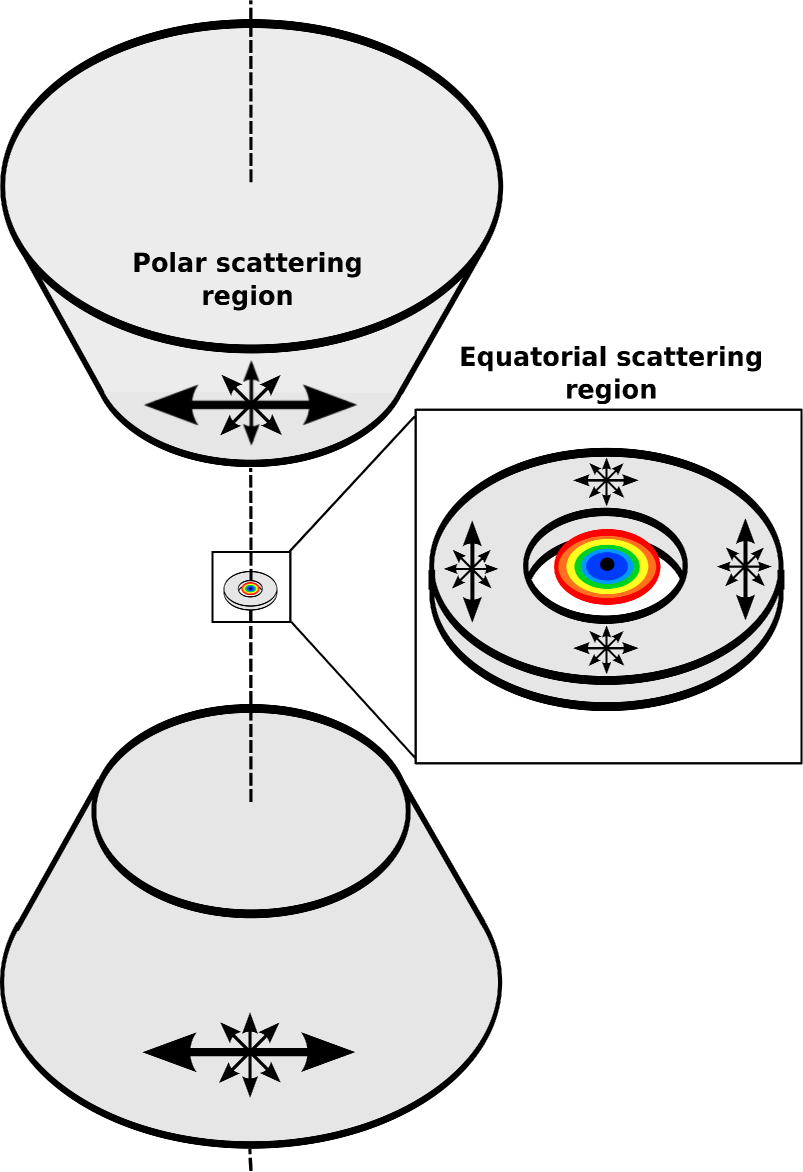
Figure 2: Schematic picture (not to scale; adapted from Smith et al. 2004) illustrating the model adopted for interpreting the quasar continuum polarization. The equatorial scattering region is compact and magnified by microlensing together with the central continuum source (the accretion disk), while the polar scattering region is more extended and not magnified. The system axis is inclined with respect to the line of sight to the observer. The arrows indicate the direction of the resulting polarization projected onto the plane of the sky for each scattering region. The equatorial scattering region produces low polarization predominantly parallel to the system symmetry axis, while the polar scattering region produces high polarization perpendicular to the system axis.

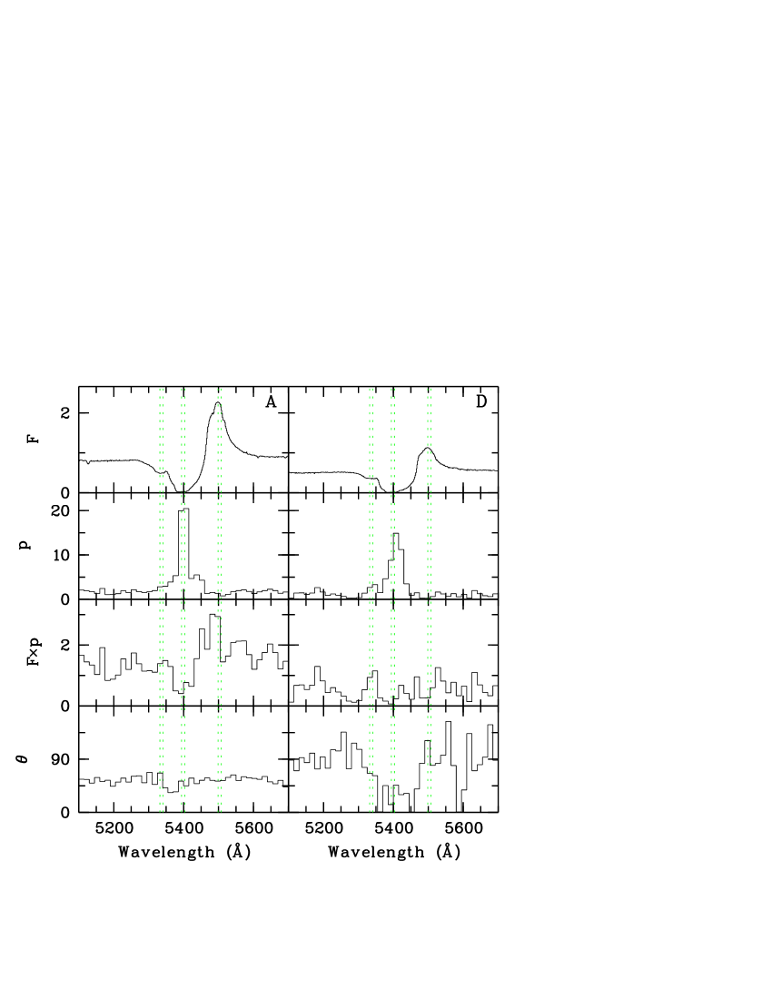
Figure 3: The polarization of the C iv line. From top to bottom, the total flux $F(\lambda)$, (in arbitrary units), the linear polarization degree $p(\lambda)$, (in %), the polarized flux $F(\lambda)\times p(\lambda)$, (in arbitrary units), and the polarization position angle $\theta(\lambda)$ (in degree). The left panel refers to image A and the right panel to image D. The position of the broad emission line, the low-velocity BAL and the high-velocity BAL are indicated.

In image D, microlensing magnifies the contribution of the compact polarized continuum by a factor $\sim$ 2 with respect to image A, which results in a rotation of the continuum polarization angle from $\sim$ 55° to $\sim$ 85°. In the BAL trough, the light from the compact source is blocked and the polarization angle jumps to the polarization angle of the polar-scattered continuum, i.e., $\sim$ 35°. The polarization angle rotates over the 5310-5470 Å wavelength range, which corresponds to the full intrinsic absorption line extracted in Paper I.

The emission lines are not significantly affected by microlensing (Papers I and II). They should then arise from a region larger than the compact continuum (larger than 20 light days according to O’Dowd et al. odo15 (2015)). Since they appear in the polarized flux and show a polarization degree lower than the continuum, they should come from a region roughly cospatial with the extended scattering region, as their lower polarization is due to geometric dilution (Goodrich and Miller goo95 (1995)). Weakly polarized emission lines dilute the continuum polarization and only slightly affect its polarization angle. In image D, the compact continuum is magnified and the relative contribution of the emission lines is smaller.

4 Discussion

Our observations suggest the existence of two scattering regions producing roughly perpendicularly polarized continua. The microlensed polarized continuum comes from a region close to the accretion disk in the equatorial plane producing polarization predominantly parallel to the accretion disk axis, while the non-microlensed one comes from an extended polar region producing perpendicular polarization. In this scenario, we would expect the accretion disk axis and thus the radio jet to have position angles close to $\sim$ 115°. Unfortunately, no clear information on the object morphology is available

Since an equatorial BAL wind can originate from the accretion disk (Murray et al. mur95 (1995)), the polarization of the compact continuum could be due to electron scattering at the base of the wind, as proposed by Wang et al. (wan05 (2005, 2007)). Observed at high inclination, this ring-like region predominantly produces parallel polarization. Both the central unpolarized source and this compact scattering region are microlensed in image D. On the other hand, the extended polar scattering region could be related to polar BAL and/or BEL regions (e.g., Ogle ogl97 (1997); Korista and Ferland kor98 (1998); Ghosh and Punsly gho07 (2007)), in agreement with the two-component wind structure proposed in Paper I (see also Borguet and Hutsemékers bor10 (2010), and Borguet bor09 (2009)). Finally, resonance scattering in the equatorial and polar BAL flows could fill in the red part of the absorption troughs with light polarized at the same position angle as the continuum, so that a significant rotation of the polarization angle is only observed on the blue side of the main absorption trough. Detailed modeling would be needed to test these hypotheses.

In Paper II we found that, in 2011, the highest velocity BAL trough absorbs the extended continuum more strongly than the compact continuum. In that case, we would expect the polarization angle to jump toward the value of the compact continuum, i.e., $\sim$ 115°, in that trough. This is not observed (Fig. 3). This may indicate that the part of the extended scattering region that contributes the most to the polarization differs from the part of the extended region that suffers strong absorption in the highest velocity BAL trough. Alternatively, the high-velocity part of the wind can be more clumpy than the low-velocity part. The secular decrease of the high-velocity absorption trough (Paper I and II) could be due to clouds moving out of the line of sight (Capellupo et al. cap14 (2014)), thus affecting the light from the compact region more strongly than the light from the extended region. In that case, absorbing clouds could preferentially uncover the part of the ring-like compact polarization source that produces polarization perpendicular to the system axis, so that the polarization angle in the high-velocity trough remains roughly unchanged.

5 Conclusions

We have obtained spectropolarimetric observations of the four images of the gravitationally lensed BAL quasar H1413+117. We found that the polarization of image D, which is microlensed, is significantly different from the polarization of image A, which is essentially unaffected by microlensing.

The observations can be consistently interpreted by assuming that the polarized continuum comes from two regions, producing roughly perpendicular polarizations: a compact one located in the equatorial plane close to the accretion disk and an extended one located along the polar axis. Our results provide further evidence for the existence of a region in H1413+117 that is more extended than the accretion disk and that significantly contributes to the observed continuum. Our findings allow us to identify this as a polar-scattering region.

Appendix A A simple model for the polarization of the continuum

We consider two sources of continuum polarization. The compact source ($c$) is microlensed by a factor $\mu$ and the extended source ($e$) is not microlensed. Both are macrolensed by a factor $M$. We write for images 1 and 2

$$F_{1} = M\,F_{e}+M\mu\,F_{c}\;,$$ (1)

$$S_{1} = M\,S_{e}+M\mu\,S_{c}\;,$$ (2)

$$F_{2} = F_{e}+F_{c}\;,$$ (3)

$$S_{2} = S_{e}+S_{c}\;,$$ (4)

where $S$ represents the Stokes fluxes $Q$ or $U$. We assumed that the compact source is magnified by the microlensing caustic network without spatial distortions modifying its polarization. Denoting $\beta$ = $F_{e}/F_{c}$, the flux ratio of the extended and the compact continua, we have

$$s_{1} = \frac{\mu\,s_{c}+\beta\,s_{e}}{\mu+\beta}\;,$$ (5)

$$s_{2} = \frac{s_{c}+\beta\,s_{e}}{1+\beta}\;,$$ (6)

where $s$ denotes the normalized Stokes parameters $q$ or $u$. These equations can be solved to express the polarization of the compact and extended continua as a function of the polarization measured in images 1 and 2, i.e.,

$$s_{e} = \frac{\mu\,(1+\beta)\,s_{2}-(\mu+\beta)\,s_{1}}{\beta\,(\mu-1)}\;,$$ (7)

$$s_{c} = \frac{(\mu+\beta)\,s_{1}-(1+\beta)\,s_{2}}{\mu-1}\;.$$ (8)

The polarization degrees and polarization angles can finally be computed using $p_{x}=\sqrt{q_{x}^{2}+u_{x}^{2}}$ and $\theta_{x}=1/2\,\arctan\,(u_{x}/q_{x})$, where $x$ = $c$ or $e$ for either the compact or the extended continuum.