Scalable posterior approximations for large-scale Bayesian inverse problems via likelihood-informed parameter and state reduction

Abstract

Two major bottlenecks to the solution of large-scale Bayesian inverse problems are the scaling of posterior sampling algorithms to high-dimensional parameter spaces and the computational cost of forward model evaluations. Yet incomplete or noisy data, the state variation and parameter dependence of the forward model, and correlations in the prior collectively provide useful structure that can be exploited for dimension reduction in this setting—both in the parameter space of the inverse problem and in the state space of the forward model. To this end, we show how to jointly construct low-dimensional subspaces of the parameter space and the state space in order to accelerate the Bayesian solution of the inverse problem. As a byproduct of state dimension reduction, we also show how to identify low-dimensional subspaces of the data in problems with high-dimensional observations. These subspaces enable approximation of the posterior as a product of two factors: (i) a projection of the posterior onto a low-dimensional parameter subspace, wherein the original likelihood is replaced by an approximation involving a reduced model; and (ii) the marginal prior distribution on the high-dimensional complement of the parameter subspace. We present and compare several strategies for constructing these subspaces using only a limited number of forward and adjoint model simulations. The resulting posterior approximations can rapidly be characterized using standard sampling techniques, e.g., Markov chain Monte Carlo. Two numerical examples demonstrate the accuracy and efficiency of our approach: inversion of an integral equation in atmospheric remote sensing, where the data dimension is very high; and the inference of a heterogeneous transmissivity field in a groundwater system, which involves a partial differential equation forward model with high dimensional state and parameters.

1 Introduction

Inverse problems convert indirect observations into useful characterizations of the parameters of a physical system. These parameters are related to the observations by a forward model, which often is expressed as a system of ordinary or partial differential equations (PDEs) or as an integral equation. Observations are inevitably corrupted by noise, and the unknown model parameters may be high-dimensional or infinite-dimensional in principle. Solution of the inverse problem is thus classically ill-posed: many feasible realizations of the parameters may be consistent with the data, and small perturbations in the data may lead to large perturbations in unregularized parameter estimates. Rather than seeking regularized point estimates, the Bayesian approach [1, 2, 3] casts the inverse solution as the posterior probability distribution of the model parameters conditioned on data, and introduces regularization in the form of prior information. It thus provides a means of combining prior knowledge, the data and forward model, and a stochastic description of measurement and/or model errors; the result is a principled quantification of uncertainty in parameters and in parameter-dependent predictions. Characterizing the posterior, however, is in general a computationally challenging task. The workhorses of Bayesian computation in this context are Markov chain Monte Carlo (MCMC) methods [4, 5, 6], originating with the Metropolis-Hastings algorithm [7, 8].

A central challenge in the application of MCMC methods to inverse problems is poor scaling of computational effort with parameter dimension and with the size of the forward model. High-dimensional parameters frequently represent the discretization of a spatial field (e.g., the permeability field of a porous medium) that is the target of inference. Yet the efficiency of many standard MCMC methods degrades with parameter dimension [9, 10, 11, 12, 13]; longer mixing times for MCMC chains then demand more posterior evaluations to estimate posterior expectations with any given accuracy. Similarly, many forward models of interest have high-dimensional states—resulting, for instance, from finite-element discretizations of PDEs, where many degrees of freedom are needed to resolve the relevant physics accurately. The computational expense of each forward model evaluation scales at least linearly with the dimension of model state (e.g., when the solution of a linear system is required). Another important but often-neglected computational expense in MCMC methods is the proposal process: the cost of generating random variables and calculating the candidate step often scales at least linearly with the parameter dimension.

To overcome these twin challenges—parameter dimension and forward model cost—this paper proposes a likelihood-informed approach for identifying and exploiting low-dimensional structure in both the parameter space and the model state space of inverse problems. Our approach integrates and extends two lines of research: the likelihood-informed parameter dimension reduction of [14, 15] and the data-driven model reduction of [16]. By simultaneously considering the limited accuracy or influence of the observations, the smoothing properties of the forward model, and the covariance structure of the prior, the former identifies a low-dimensional likelihood-informed parameter subspace (LIPS) where the influence of the likelihood on the posterior dominates that of the prior. Given this subspace, one can approximate the full posterior as the product of a low-dimensional posterior on the LIPS and the marginalization of the prior onto the complement of the LIPS. The latter term can be characterized analytically or with perfectly independent samples. Evaluation of the posterior density restricted to the LIPS is still computationally expensive, however, as it involves the full forward model. Our second step accelerates these evaluations by projecting [18, 19, 20, 21] the forward model—with input parameters restricted to the LIPS—onto a low-dimensional state subspace. This subspace is called the likelihood-informed state subspace (LISS), as it captures variations in the model state associated with the LIPS-projected posterior. This model reduction approach extends the data-driven model reduction ideas of [16] by not only exploiting posterior concentration, but also avoiding consideration of input parameter directions that ultimately will not be data-informed. Finally, we combine these approximations together: the reduced-order model resulting from projection onto the LISS is substituted into the product-form approximation of the posterior described above. The resulting jointly-approximated posterior is inexpensive to evaluate and to sample, with a computational cost that is independent of the dimension of the full model state or the parameters. Indeed, this cost scales only with the dimensions of the LIPS and the LISS, which are in a sense the intrinsic dimensions of the problem.

As a byproduct of state reduction, we describe new approaches for efficiently handling and reducing high-dimensional data sets in inverse problems; these approaches are potentially useful in “big data” settings. While the jointly-approximated posterior achieves excellent accuracy in our numerical examples, we also discuss how to use it as a proposal distribution in importance sampling or delayed-acceptance MCMC [22, 23] for the purpose of “exact” sampling—i.e., the computation of expectations with respect to the full posterior—if desired. To ensure convergence in this setting, we introduce a special treatment of the tails of the jointly-approximated posterior.

Previous work has also investigated the idea of combining parameter reduction with model reduction or other forms of surrogate modeling in order to approximate posterior distributions. One early effort is [24], which constructs a reduced parameter basis using the truncated Karhunen-Lòeve (KL) expansion [25, 26] of the prior covariance, and then uses generalized polynomial chaos expansions [27, 28, 29] to build a surrogate of the full model. The same KL-based parameter reduction technique has also been combined with projection-based model reduction to accelerate posterior evaluations; examples include [30] and [16]. Similarly, [31] combines a process convolution model [32] of the parameters with a sparse grid approximation of the forward model. A different approach in [33] simultaneously identifies reduced subspaces for both the parameters and the state, by solving a sequence of model-constrained optimization problems penalized by the prior. In general, all these earlier approaches seek a truncation of the parameter dimension and then accelerate forward model evaluations over the reduced parameter subspace using surrogates. The smoothness of the prior plays a crucial role in these approaches, either for avoiding large KL truncation errors or for promoting convergence of the model-constrained optimization. In practice, this requirement can impose significant restrictions on the choice of priors. Our approach is fundamentally different in several respects. First, our posterior approximation is based on capturing the change from the prior to the posterior within the LIPS, rather than directly truncating the parameter dimension of the problem. Second, model reduction using the LISS only captures the state variations that are relevant to the change from prior to posterior; this “localization” strategy is key to the successful construction of reduced-order models for high-dimensional parameterized systems. Furthermore, our jointly-approximated posterior is not singular with respect to the full posterior, and can thus be used to drive exact sampling schemes (e.g., importance sampling as mentioned above).

The rest of this paper is organized as follows. In Section 2, we review the Bayesian formulation of inverse problems. In Section 3, we introduce the concept of joint posterior approximation using reduced parameter and state subspaces, then detail various strategies and practical algorithms for constructing this approximation and for exploring the full posterior. In Section 4, we demonstrate various aspects of our proposed approach using an atmospheric remote sensing problem, comparing different strategies for subspace identification and for the reduction of high-dimensional data. In Section 5, we apply our joint posterior approximation approach to the inference of the transmissivity field of a groundwater aquifer. Section 6 offers concluding remarks.

2 Bayesian formulation for inverse problems

We begin by constructing the forward model. Consider a numerical discretization of the system of interest, described by a nonlinear equation

$$A(u,x)=0,$$ (1)

where $u\in\mathbb{U}\subseteq{}^{m}$ and $x\in\mathbb{X}\subseteq{}^{n}$ are the $m$-dimensional state vector and the $n$-dimensional parameter vector, respectively. The goal of an inverse problem is to infer the unobservable parameters $x$ from noisy partial observations of the states $u$, given by

$$y_{\rm obs}=C(u,x)+e\,.$$ (2)

Here $C$ is a discretized observation operator mapping from the states and parameters to the observables, and $e$ is a random variable representing noise and/or model error, which appear additively. The system model $A(u,x)=0$ and observation model $C(u,x)$ together define a forward model $y=F(x)$ that maps the unknown parameter to the observable model outputs. We note that although the forward model defined by (1) and (2) is induced by a stationary problem, the methodology presented in this paper is also applicable to time-dependent systems.

To formulate the inverse problem in a Bayesian setting, we model the parameter $x$ as a random variable, endow it with a prior distribution, and then characterize its posterior distribution given a realization of the data, $y_{\rm obs}\in\mathbb{Y}\subseteq{}^{d}$:

$$\pi(x|y_{\rm obs})\propto\mathcal{L}(y_{\rm obs}|x)\pi_{0}(x).$$ (3)

Here, we assume that all distributions have densities with respect to Lebesgue measure. The posterior density above is the product of two terms: the prior density $\pi_{0}(x)$, which models knowledge of the parameters before the data are observed, and the likelihood function $\mathcal{L}(y_{\rm obs}|x)$, which describes the probability distribution of $y_{\rm obs}$ for a given $x$.

We develop our formulation in the setting of a multivariate Gaussian prior $\mathcal{N}(\mu_{\rm pr},\Gamma_{\rm pr})$, where the covariance matrix $\Gamma_{\rm pr}$ might also be specified by its inverse $\Gamma_{\rm pr}^{-1}$, commonly referred to as the precision matrix. The additive observational noise is taken to be a zero mean Gaussian distribution, i.e., $e\sim\mathcal{N}(0,\Gamma_{\rm obs})$. Given the weighted inner product $\langle y_{1},y_{2}\rangle_{\Gamma_{\rm obs}}=\langle y_{1},\Gamma_{\rm obs}^{-1}y_{2}\rangle$ and the induced norm $\|y\|_{\Gamma_{\rm obs}}=\sqrt{\langle y,y\rangle_{\Gamma_{\rm obs}}}$, we can define a data-misfit function

$$\eta(x)=\frac{1}{2}\left\|F(x)-y_{\rm obs}\right\|^{2}_{\Gamma_{\rm obs}}.$$ (4)

The likelihood function is thus proportional to $\exp\left(-\eta(x)\right)$. The Gaussian settings used here can be generalized to non-Gaussian priors, e.g., log-normal distributions, with an appropriate transformation or change of variables to a Gaussian. Additive but non-Gaussian noise can be handled similarly. These transformations may introduce additional nonlinearity in the forward model.

Note that the unknown parameters and the model states are in principle functions of space and/or time, and that the finite-dimensional representations above are the result of numerical discretization. If one considers progressively refining the parameter discretization, however, the posterior distribution does not have a density with respect to Lebesgue measure at the infinite-dimensional limit. However, for inverse problems with properly chosen Gaussian priors—e.g., a covariance operator that is self-adjoint, positive definite, and trace-class—and a forward model satisfying certain regularity conditions—e.g., appropriately bounded [3] and locally Lipschitz—the posterior has a density with respect to the prior and yields a full measure at the infinite-dimensional limit. In this case, Bayes’ rule in (3) is expressed as the Radon-Nikodym derivative of the posterior with respect to the prior. We refer the readers to [3] and references therein for more details. Since we aim to approximate the posterior distribution defined by given discretizations of the parameters, a finite-dimensional forward model, and the associated prior, we adopt the finite-dimensional representation of the posterior as our starting point in this paper. This finite-dimensional posterior can be derived either from a consistent discretization of an infinite-dimensional inverse problem or from some other existing numerical models that are not necessarily well-defined in the infinite-dimensional limit.

3 Posterior approximation via dimension reduction

In this section, our first objective is to reduce the algorithmic complexity of posterior sampling by identifying a likelihood-informed parameter subspace (LIPS) that captures parameter directions where the change from prior to posterior is most significant. We will then decompose the posterior into the product of (i) a low-dimensional distribution, defined on the LIPS, that is analytically intractable and therefore must be sampled; and (ii) a higher-dimensional but analytically tractable marginal of the prior distribution on the complement of the LIPS. To accelerate the forward model evaluations required when sampling the first term of this product decomposition, we will identify a low-dimensional subspace of the forward model state—the likelihood-informed state subspace (LISS)—and construct a reduced version of the forward model accordingly. Introducing this reduced model into the product decomposition yields the jointly-approximated posterior distribution described in the introduction. At the end of this section, we will describe and compare various sampling strategies for constructing the LISS and LIPS, and hence the jointly-approximated posterior. We will also discuss methods for exploring the full posterior distribution, given the preceding approximations.

3.1 Data-informed parameter reduction

Inverse problems very often involve some combination of a smoothing forward model, limited or noisy observations, and correlations in the prior. When any of these factors is present, the data will not equally inform all directions in the parameter space. We may be able to explicitly project the argument of the likelihood function onto a lower-dimensional subspace of the parameter space without losing much information. Our objective here is to find an $r$-dimensional LIPS, denoted by $\mathbb{X}_{r}$, to capture the parameter directions where the likelihood is “most informative” relative to the prior. This notion will be defined more precisely below.

3.1.1 Parameter-reduced posterior

Consider a rank-$r$ projector $\Pi_{r}$ whose range is the LIPS, i.e., $\mathbb{X}_{r}=\operatorname{range}(\Pi_{r})$. We approximate the posterior density (3) as:

$$\hat{\pi}(x|y_{\rm obs})\propto\mathcal{L}\left(y_{\rm obs}|\Pi_{r}x\right)\pi_{0}(x),$$ (5)

where $\mathcal{L}\left(y_{\rm obs}|\Pi_{r}x\right)$ is an approximation to the original likelihood function $\mathcal{L}\left(y_{\rm obs}|x\right)$. We require the projector $\Pi_{r}$ to be orthogonal with respect to the inner product induced by the prior covariance $\langle x_{1},x_{2}\rangle_{\Gamma_{\rm pr}}=\langle x_{1},\Gamma_{\rm pr}^{-1}x_{2}\rangle$. This requirement is essential to constructing a tractable product-form approximation of the posterior.

Definition 3.1 (Parameter space projectors).

Suppose the subspace $\mathbb{X}_{r}$ is spanned by a basis $\Phi_{r}\in{}^{n\times r}$ that is orthogonal with respect to the inner product $\langle\cdot,\cdot\rangle_{\Gamma_{\rm pr}}$, i.e., $\langle\Phi_{r},\Phi_{r}\rangle_{\Gamma_{\rm pr}}=I_{r}$, where $I_{r}$ is the $r$-by-$r$ identity matrix. Define the matrix $\Xi_{r}\in{}^{n\times r}$ such that $\Xi_{r}^{\top}\Phi_{r}=I_{r}$. Then the projectors

$$\Pi_{r}=\Phi_{r}\Xi_{r}^{\top}\quad{\rm and}\quad\Pi_{\perp}=I-\Pi_{r},$$

are orthogonal with respect to $\langle\cdot,\cdot\rangle_{\Gamma_{\rm pr}}$. Moreover, the $(n-r)$-dimensional subspace $\mathbb{X}_{\perp}=\operatorname{range}(\Pi_{\perp})$ is the orthogonal complement of $\mathbb{X}_{r}$ with respect to $\langle\cdot,\cdot\rangle_{\Gamma_{\rm pr}}$. We can choose a basis $\Phi_{\perp}\in{}^{n\times(n-r)}$ such that $[\Phi_{r},\Phi_{\perp}]$ forms a complete orthogonal system in ⁿ with respect to $\langle\cdot,\cdot\rangle_{\Gamma_{\rm pr}}$, and thus the projector $\Pi_{\perp}$ can be written as $\Pi_{\perp}=\Phi_{\perp}\Xi_{\perp}^{\top}$, where $\Xi_{\perp}\in{}^{n\times(n-r)}$ is the matrix such that $\Xi_{\perp}^{\top}\Phi_{\perp}=I_{\perp}$.

Using the projectors defined above, the parameter $x$ can be decomposed as $x=\Pi_{r}x+\Pi_{\perp}x$, where each projection can be represented as the linear combination of the corresponding basis vectors. Consider parameters $x_{r}$ and $x_{\perp}$ that are the weights associated with the bases $\Phi_{r}$ and $\Phi_{\perp}$, respectively. Then we can define the following pair of linear transformations between $x$ and $(x_{r},x_{\perp})$:

$$x=\left[\Phi_{r}\;\Phi_{\perp}\right]\left[\begin{array}[]{l}x_{r}\\ x_{\perp}\end{array}\right]\quad{\rm and}\quad\left[\begin{array}[]{l}x_{r}\\ x_{\perp}\end{array}\right]=\left[\Xi_{r}\;\Xi_{\perp}\right]^{\top}x.$$ (6)

Lemma 3.2.

Given the decomposition $x=\Phi_{r}x_{r}+\Phi_{\perp}x_{\perp}$ defined in (6), the prior distribution can be decomposed into the product form $\pi_{0}(x)\propto\pi_{0}(x_{r})\pi_{0}(x_{\perp})$, where $\pi_{0}(x_{r})=\mathcal{N}(\Xi_{r}^{\top}\mu_{\rm pr},I_{r})$ and $\pi_{0}(x_{\perp})=\mathcal{N}(\Xi_{\perp}^{\top}\mu_{\rm pr},I_{\perp})$.

Applying the linear transformation (6) and Lemma 3.2, the parameter-approximated posterior (5) can be written as

$$\hat{\pi}(x|y_{\rm obs})\propto\hat{\pi}(x_{r},x_{\perp}|y_{\rm obs})=\pi(x_{r}|y_{\rm obs})\pi_{0}(x_{\perp}),$$ (7)

which is the product of the parameter-reduced posterior

$$\pi(x_{r}|y_{\rm obs})\propto\mathcal{L}\left(y_{\rm obs}|\Phi_{r}x_{r}\right)\pi_{0}(x_{r}),$$ (8)

and the complement prior $\pi_{0}(x_{\perp})$. In this product-form approximation, the prior-to-posterior update is captured entirely by the parameter-reduced posterior. Approximations of this form naturally yield a scalable posterior exploration scheme: the high-dimensional complement prior $\pi_{0}(x_{\perp})$ is analytically tractable, and the remaining challenge is to explore the analytically intractable but low-dimensional parameter-reduced posterior (8). Of course, this construction rests on identifying the LIPS basis $\Phi_{r}$. In the rest of this subsection, we will discuss several ways to construct the LIPS by balancing the influence of the prior and the likelihood.

Remark 3.3.

It is usually not feasible to compute and store the high-dimensional basis $\Phi_{\perp}\in{}^{n\times(n-r)}$. In fact, the construction of the parameter-approximated posterior (7) only requires the low-dimensional LIPS basis $\Phi_{r}$ in order to construct the parameter-reduced posterior. Operations involving the complement subspace $\mathbb{X}_{\perp}$ are performed using the projector $\Pi_{\perp}=I-\Pi_{r}$ rather than the high-dimensional basis $\Phi_{\perp}$.

3.1.2 Likelihood-informed parameter subspace

In previous work [14, 34, 35, 36, 37], the Hessian of the data-misfit function (4) (in particular, the Gauss-Newton approximation $H(x)$ of the Hessian) is used to quantify the local impact of the likelihood, relative to the prior, along a parameter direction $\varphi$. This notion of relative impact is captured via the local Rayleigh ratio

$$\mathcal{R}(\varphi;x)=\frac{\langle\varphi,H(x)\varphi\rangle}{\langle\varphi,\Gamma_{\rm pr}^{-1}\varphi\rangle},$$ (9)

which is maximized (over successively smaller subspaces $\operatorname{span}^{\bot}{(\varphi_{j})_{j<i}}$) by generalized eigenvectors of the matrix pencil $(H(x),\Gamma_{\rm pr}^{-1})$

$$H(x)\varphi_{i}=\gamma_{i}\Gamma_{\rm pr}^{-1}\varphi_{i}.$$ (10)

The largest eigenvalues of (10) correspond to parameter directions along which the local curvature of the log-posterior density is more constrained by the log-likelihood than by the log-prior. Conversely, eigendirections associated with the smallest eigenvalues correspond to directions along which the likelihood is essentially flat, and hence where the posterior is (locally) determined by the prior.

Given the local Gauss-Newton approximation of the Hessian, $H(x)$, we can define a local Gaussian approximation of the posterior with covariance $\Gamma_{\rm pos}(x):=(H(x)+\Gamma_{\rm pr}^{-1})^{-1}$. This covariance can be written as a low-rank update of the prior covariance:

$$\Gamma_{\rm pos}(x)\approx\Gamma_{\rm pos}^{(l)}=\Gamma_{\rm pr}-\sum_{i=1}^{l}\frac{\gamma_{i}}{\gamma_{i}+1}\varphi_{i}\varphi_{i}^{\top}\,,$$ (11)

which is in general approximate for $l<n$. Here $\varphi_{i}$ and $\gamma_{i}$ are eigenvectors and eigenvalues from (10), which depend on the parameter $x$. In this approximation, the basis $\{\varphi_{1},\ldots,\varphi_{l}\}$ characterizes the prior-to-posterior update at a given $x$.

This low-rank update was first used in [34] for computing and factorizing the posterior covariance in large-scale linear inverse problems. Spantini et al. [14] proved the optimality of this approximation at any given $l$, for linear inverse problems, in the sense of minimizing the Förstner-Moonen [38] distance from the exact posterior covariance matrix over the class of positive definite matrices that are rank-$l$ negative semidefinite updates of the prior covariance. For nonlinear inverse problems, given the posterior mode (i.e., the maximum a posteriori (MAP) estimator)

$$x_{\rm MAP}=\operatorname*{arg\,max}_{x}\pi(x|y_{\rm obs}),$$

the local Gaussian approximation (11) centered at $x_{\rm MAP}$ yields a Laplace approximation of the posterior:

$$\pi(x|y_{\rm obs})\approx\pi_{\rm L}(x)=\mathcal{N}\left(x_{\rm MAP}\,,\,\Gamma_{\rm pr}-\sum_{I=1}^{l}\frac{\gamma_{i}}{\gamma_{i}+1}\varphi_{i}\varphi_{i}^{\top}\right).$$ (12)

For unimodal and nearly Gaussian posteriors, the Laplace approximation might be used directly as a surrogate for the posterior, as in [36]; alternatively, it can be used as a fixed preconditioner for MCMC sampling, as in the stochastic Newton method of [37]. We will use the Laplace approximation as a component of certain subspace construction strategies, described in the next subsection.

We wish to construct the parameter-approximated posterior (7) for nonlinear inverse problems, and thus must extend beyond Gaussian approximations. Since the Hessian varies over the parameter space for nonlinear forward models, the likelihood-informed directions also vary with $x$ and are embedded in some nonlinear manifold. To build a global linear subspace—the LIPS—that captures the majority of this nonlinear manifold, Cui et al. [15] extends the pointwise criterion (9) into the expected value of the Rayleigh quotient over the posterior

$$\mathbb{E}_{\pi(x|y_{\rm obs})}\left[\mathcal{R}(\phi;x)\right]=\frac{\langle\phi,S_{\rm post}\,\phi\rangle}{\langle\phi,\Gamma_{\rm pr}^{-1}\phi\rangle},$$ (13)

where $S_{\rm post}$ is the posterior expectation of the Gauss-Newton approximation of the Hessian (GNH):

$$S_{\rm post}=\int_{\mathbb{X}}H(x)\,\pi(dx|y_{\rm obs}).$$ (14)

This way, the LIPS can be obtained through the eigendecomposition of the matrix pencil $\left(S_{\rm post},\Gamma_{\rm pr}^{-1}\right)$,

$$S_{\rm post}\,\phi_{i}=\lambda_{i}\Gamma_{\rm pr}^{-1}\phi_{i}.$$ (15)

The eigenvectors $\{\phi_{1},\ldots,\phi_{r}\}$ correspond to the $r$ leading eigenvalues of (15), such that $\lambda_{1}\geq\lambda_{2}\geq\ldots\geq\lambda_{r}\geq\tau_{\rm g}>0$, span the LIPS. Here the truncation threshold $\tau_{\rm g}$ is usually set to a value less than one, e.g., $\tau_{\rm g}=10^{-1}$, thus only removing parameter directions where the impact of the likelihood is significantly smaller than that of the prior.

The evaluation of the expected GNH (14) should be carried out adaptively during posterior exploration. In particular, we consider approximating $S_{\rm post}$ using Monte Carlo integration,

$$\widehat{S}_{\rm post}=\frac{1}{N}\sum_{k=1}^{N}H(x^{(k)}),$$

where $x^{(k)}\sim\pi(x|y_{\rm obs})$, $k=1\ldots N$, are posterior samples adaptively selected during posterior exploration. Section 3.3 will describe how we fit this task into an adaptive sampling framework where posterior exploration and posterior approximation are carried out simultaneously.

Lemma 3.4.

The eigenvectors $\{\phi_{1},\ldots,\phi_{r}\}$ are linearly independent and form a LIPS basis $\Phi_{r}=[\phi_{1},\ldots,\phi_{r}]$ that is orthogonal with respect to the inner product $\langle\cdot,\cdot\rangle_{\Gamma_{\rm pr}}$.

Proof.

The result directly follows from the fact that the estimated expected GNH $\widehat{S}_{\rm post}$ is symmetric positive semidefinite and the prior covariance $\Gamma_{\rm pr}$ is symmetric positive definite. See Theorem 15.3.3 of [39] for details. ∎

As a consequence of Lemma 3.4, we can construct the matrix $\Xi_{r}=\Phi_{r}\,(\Phi_{r}^{\top}\,\Phi_{r})^{-1}$, such that $\Xi_{r}^{\top}\Phi_{r}=I_{r}$, and the projector $\Pi_{r}=\Phi_{r}\Xi_{r}^{\top}$ as in Definition 3.1. This way, the parameter-approximated posterior (7) and parameter-reduced posterior (8) can be defined.

3.1.3 Parameter subspace identification: choice of reference distribution

The LIPS basis discussed above results from balancing the influence of the prior and the likelihood over the support of the posterior. It is also possible to quantify this relative influence using expectations of the local Rayleigh quotient over other reference distributions. Depending on the choice of reference distribution, the local likelihood-informed directions—summarized by the local Rayleigh quotient—are weighed differently in the resulting LIPS. Furthermore, the involvement of the observed data set in the reference distribution affects how computational resources might be allocated to LIPS construction. If the observed data are not involved in the reference distribution, the evaluation of the expectation can be performed once for a particular combination of forward model and prior, and reused for different data sets. This way, LIPS construction is decoupled from any particular data set, and we consider it to be an offline procedure. In contrast, if the reference distribution involves the observation—e.g., if it is the posterior—the resulting expectation evaluation is an online procedure, as the LIPS basis must be recomputed for each new data set.

One obvious candidate for the reference distribution is the prior, which leads to a LIPS basis that is constructed from the eigendecomposition of the matrix pencil $\left(S_{\rm pr},\Gamma_{\rm pr}^{-1}\right)$, where

$$S_{\rm pr}=\int_{\mathbb{X}}H(x)\,\pi_{0}(dx),$$

is the expected GNH over the prior. As discussed above, using the prior as a reference distribution leads to an offline procedure for parameter dimension reduction.

Alternatively, we can set the reference distribution to be the Laplace approximation (12), which is an inexpensive and easy-to-sample surrogate for the posterior. This way, the LIPS can be obtained from the eigendecomposition of the pencil $\left(S_{\rm L},\Gamma_{\rm pr}^{-1}\right)$, where

$$S_{\rm L}=\int_{\mathbb{X}}H(x)\,\pi_{\rm L}(dx).$$

Although samples can be directly drawn from the Laplace approximation, this choice of reference constitutes an online approach, since the Laplace approximation is data-dependent.

All of the LIPS bases discussed above are orthogonal with respect to the inner product $\langle\cdot,\cdot\rangle_{\Gamma_{\rm pr}}$, since they result from generalized eigenproblems involving $\Gamma_{\rm pr}^{-1}$. We note that other choices of reduced parameter basis can also lead to the product-form approximated posterior (7), provided that the basis is orthogonal with respect to $\langle\cdot,\cdot\rangle_{\Gamma_{\rm pr}}$. For instance, the basis defined by the truncated Karhunen-Loève expansion of the prior covariance [24] also satisfies this property.

Table 1: Summary of parameter dimension reduction methods discussed in Section 3.1.3: the associated eigendecomposition, whether the process is offline/online, and whether adaptive sampling is required.

Method	Eigendecomposition		Online/offline	Adaptive sampling?
Posterior-LIPS	$\left(S_{\rm post},\Gamma_{\rm pr}^{-1}\right)$	$S_{\rm post}=\int_{\mathbb{X}}H(x)\pi(dx|y_{\rm obs})$	online	yes
Laplace-LIPS	$\left(S_{\rm L},\Gamma_{\rm pr}^{-1}\right)$	$S_{\rm L}=\int_{\mathbb{X}}H(x)\pi_{\rm L}(dx)\;\,$	online	no
Prior-LIPS	$\left(S_{\rm pr},\Gamma_{\rm pr}^{-1}\right)$	$S_{\rm pr}=\int_{\mathbb{X}}H(x)\pi_{0}(dx)\;\;\,$	offline	no
Prior-KL	$\Gamma_{\rm pr}$	–	offline	no

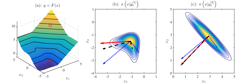
Figure 1: Illustration of Example 3.5. (a) Forward model, with two different observations $y_{\rm obs}^{(1)}$ and $y_{\rm obs}^{(2)}$ marked by the triangle and the circle, respectively. (b) Contours of the posterior density $\pi(x|y_{\rm obs}^{(1)})$. (c) Contours of the posterior density $\pi(x|y_{\rm obs}^{(2)})$. On (b) and (c), the parameter bases computed using posterior-LIPS, Laplace-LIPS, and prior-LIPS are depicted by the solid, dashed, and dotted lines, respectively.

All of the parameter subspace identification techniques presented here can be interpreted as the result of an eigendecomposition. For each technique, Table 1 summarizes the specific form of eigendecomposition, whether reduction is offline/online, and whether adaptive sampling is required. We compute the expected Hessians required for both Prior-LIPS and Laplace-LIPS using Monte Carlo integration, where samples can be directly generated from the prior and the Laplace approximation. These Hessian evaluations are therefore embarrassingly parallel. Posterior-LIPS, on the other hand, requires posterior sampling; we defer a discussion of the associated adaptive framework to Section 3.3. We also note that Prior-KL is less computationally demanding than the other methods discussed here, as it only involves an eigendecomposition of the prior covariance.

Example 3.5 (Parameter reduction with different reference distributions).

To demonstrate the properties of different parameter reduction approaches, we consider a two-dimensional inverse problem with the following scalar-valued forward model:

$$F(x):=\frac{1}{2}\left[\left(\operatorname{erf}\left(x_{1}+1\right)+1\right)\left(x_{1}+1\right)+\left(\operatorname{erf}\left(x_{2}+1\right)+1\right)\left(x_{2}+1\right)+\left(1-\operatorname{erf}\left(x_{1}+1\right)\right)\cos(x_{2})\right].$$

We define a Gaussian observational error $e\sim\mathcal{N}(0,\sigma^{-2}I_{1})$ with $\sigma=0.25$, and a prior $\pi_{0}(x)=\mathcal{N}(0,I_{2})$. Figure 1(a) shows the response of the forward model over a range of input parameter values $(x_{1},x_{2})$. Different observations will yield posterior distributions with dramatically different shapes and orientations, due to the nonlinearity of the forward model. We consider two different observation values $y_{\rm obs}^{(1)}$ and $y_{\rm obs}^{(2)}$, generated by setting the underlying true parameter to $(-1,-2)$ and $(3,3)$, respectively. These observations are illustrated by the triangle and the circle in Figure 1(a).

As shown in Figure 1(b), the posterior distribution $\pi(x|y_{\rm obs}^{(1)})$ has strongly non-Gaussian structure in both parameter dimensions, as the observation $y_{\rm obs}^{(1)}$ falls in a regime where the forward model exhibits nonlinear behavior. In contrast, the observation $y_{\rm obs}^{(2)}$ corresponds to a parameter regime where the forward model is rather linear, and thus the posterior distribution $\pi(x|y_{\rm obs}^{(2)})$, shown in Figure 1(c), has nearly Gaussian structure.

In this example, the Prior-KL basis simply corresponds to the canonical basis of the posterior, as the prior is an independent standard Gaussian. The Prior-LIPS basis is illustrated with dotted lines and remains unchanged for both data sets, while the Posterior-LIPS basis is illustrated with solid lines and depends on the data set. The vectors corresponding to the Prior-LIPS basis and the Posterior-LIPS basis in the figure are scaled by their associated generalized eigenvalues. For the data set $y_{\rm obs}^{(2)}$, the likelihood function only informs one dimension in the parameter space, since the forward model is nearly linear in the support of the posterior. Posterior-LIPS captures this likelihood-informed subspace accurately, but Prior-LIPS does not; it suggests that two parameter directions are of comparable importance. Laplace-LIPS produces results similar to Posterior-LIPS for the data set $y_{\rm obs}^{(2)}$, but the bases generated by Laplace-LIPS and Posterior-LIPS are rather different for the data set $y_{\rm obs}^{(1)}$. This is expected, because the posterior $\pi(x|y_{\rm obs}^{(2)})$ is nearly Gaussian and well described by its Laplace approximation, whereas the posterior $\pi(x|y_{\rm obs}^{(1)})$ is strongly non-Gaussian.

As shown by the above example, all three strategies for computing the LIPS can reveal the impact of the likelihood on different parameter directions, relative to the prior. The Prior-LIPS does not depend on the data set, and hence can be constructed offline for all possible observations. Its potential drawback is that the resulting low-dimensional parameter subspace may contain directions unimportant to the posterior at hand; alternatively, some important posterior structure may be missed, due to the averaging of different Hessians over a much less concentrated parameter measure. In comparison, the online Posterior-LIPS can accurately capture likelihood-informed directions for a specific posterior distribution of interest. Depending on the shape of the posterior, Laplace-LIPS can be used either as a replacement for Posterior-LIPS when the posterior is nearly Gaussian, or as an initial guess for Posterior-LIPS that is adaptively refined (see Section 3.3).

3.2 Likelihood-informed state reduction

Although the parameter-approximated posterior $\hat{\pi}(x|y_{\rm obs})\propto\pi(x_{r}|y_{\rm obs})\pi_{0}(x_{\perp})$ enables significant reductions in the algorithmic complexity of posterior exploration, by confining sampling to a lower dimensional space, a remaining computational bottleneck is the exploration of the parameter-reduced posterior $\pi(x_{r}|y_{\rm obs})$. The cost of this exploration is dominated by forward model evaluations, and thus we turn to model reduction approaches.

3.2.1 Model reduction

In the parameter-reduced posterior, by projecting the argument of the likelihood function onto the subspace spanned by the reduced parameter basis $\Phi_{r}$, the forward model defined by (1) and (2) can be rewritten as

$$A(u,\Phi_{r}x_{r})=0,\quad{\rm and}\quad y=C(u,\Phi_{r}x_{r}).$$ (16)

To reduce the computational cost, we wish to solve a projection of the parameter-reduced forward model (16) onto a reduced dimensional state subspace. Without loss of generality, we consider the system model $A(u,x)=0$ to consist of a linear operator $L$ and a nonlinear function $f$, which take the form

$$L(x)u+f(x,u)=0.$$ (17)

Suppose that variation of the $m$-dimensional state lies within an $s$-dimensional subspace spanned by a basis $V_{s}\in{}^{m\times s}$. Then the state $u$ can be approximated by a linear combination of the reduced basis vectors, i.e., $u\approx V_{s}u_{s}$. This way, the parameter-reduced system model $A(u,\Phi_{r}x_{r})=0$ can be approximated by the following Galerkin projection:

$$\underbrace{V_{s}^{\top}L(\Phi_{r}x_{r})V_{s}}_{L_{s}(x_{r})}u_{s}+V_{s}^{\top}f(V_{s}u_{s},\Phi_{r}x_{r})=0.$$ (18)

If $s\ll m$, the dimension of the unknown state in (18) is greatly reduced compared to that of the original system (17). However, (18) cannot necessarily be solved quickly, because the reduced-order model still requires evaluating the full-scale system matrices or residual and then projecting those matrices or the residual onto the reduced state subspace. Many elements of these computations depend on the state and parameter dimension of the original system, and hence this process is typically computationally expensive (unless there is special structure to be exploited, such as affine parametric dependence). In this situation, methods such as missing point estimation [40], empirical interpolation [41], or its discrete variant [42], can be used to approximate the nonlinear term in the reduced-order model by selective spatial sampling.

We employ the discrete empirical interpolation method (DEIM) [42] to approximate the nonlinear terms of (18). Suppose that the outputs of a nonlinear function $f(V_{s}u_{s},\Phi_{r}x_{r})$ in (18) can be captured by a linear subspace spanned by the basis $\Theta_{t}\in{}^{m\times t}$. Then DEIM approximates the nonlinear term by

$$f(V_{s}u_{s},\Phi_{r}x_{r})\approx\Theta_{t}\alpha(u_{s},x_{r}).$$

Here the lower-dimensional coefficient function $\alpha(\cdot,\cdot)\in{}^{t}$ is constructed by selectively evaluating the nonlinear function $f$ at output indices $p_{1},\ldots,p_{t}$, which are chosen by a greedy procedure. This leads to a masking matrix $P_{t}=[\delta_{p_{1}},\ldots,\delta_{p_{t}}]$, where $\delta_{i}$ is the canonical basis in ^m and the matrix $P_{t}^{\top}\Theta_{t}$ is nonsingular. This way, the coefficient function can be determined by $P_{t}^{\top}f(V_{s}u_{s},\Phi_{r}x_{r})=P_{t}^{\top}\Theta_{t}\alpha(u_{s},x_{r})$, which yields

$$\alpha(u_{s},x_{r})=\left(P_{t}^{\top}\Theta_{t}\right)^{-1}P_{t}^{\top}f(V_{s}u_{s},\Phi_{r}x_{r}).$$ (19)

The resulting DEIM approximation of the reduced-order model (18) becomes

$$L_{s}(x_{r})u_{s}+V_{s}^{\top}\Theta_{t}\alpha(u_{s},x_{r})=0,$$ (20)

and the associated model outputs are

$$y=C(V_{s}u_{s},\Phi_{r}x_{r}).$$ (21)

Together (20) and (21) define a reduced-order model $y=\tilde{F}(x_{r})$ that maps a realization of the reduced parameter $x_{r}$ to an approximation of the observable model outputs. In situations where the observables are high-dimensional or the observation function $C$ involves complex nonlinear relations, we can again employ the DEIM method to approximate the observation model.

3.2.2 State subspace identification: choice of reference distribution

At the heart of model reduction is the identification of the reduced bases $V_{s}$ and $\Theta_{t}$. We employ the well-known proper orthogonal decomposition (POD) method [19, 20], also known in statistics as principal component analysis, for this task. If the parameter $x$ is distributed according to a probability distribution $p$, the eigenvectors corresponding to the leading eigenvalues of the state covariance matrix,

$$K=\int_{\mathbb{X}}u(x)u(x)^{\top}p(dx),$$ (22)

form the reduced state basis $V_{s}$ in POD. For dynamical problems, time variation of the state should also be considered, in which case the right-hand side of (22) should be integrated over both time and the parameter. The covariance matrix is often approximated empirically by full model states—commonly referred to as snapshots [19]—obtained at parameter samples drawn from the probability distribution $p$. Given $M$ samples and the snapshot matrix $U=[u(x^{(1)}),\ldots,u(x^{(M)})]$, the empirical approximation of $K$ takes the form

$$\widehat{K}=\frac{1}{M}U\,U^{\top}.$$

If the sample size is much smaller than the state dimension, i.e., $M\ll m$, the singular value decomposition (SVD) of $U$ provides an effective way of computing the reduced basis $V_{s}$. The basis $\Theta_{s}$ can be constructed in a similar fashion.

As in the parameter reduction problem, the choice of an appropriate reference probability distribution for the parameters $x$ is also essential to identifying the reduced state subspace. Using the construction of the basis $V_{s}$ as an example, we now discuss various choices of reference distribution. In the inverse problems literature, one common choice is the prior distribution [43, 44, 30], which leads to the state covariance

$$K_{\rm pr}=\int_{\mathbb{X}}u(x)u(x)^{\top}\pi_{0}(dx).$$ (23)

Alternatively, Cui et al. [16] suggest constructing the reduced-order model over the support of the posterior rather than the prior. The size and accuracy of the resulting reduced-order model can scale better with parameter dimension than those of a reduced-order model built from the prior, since the posterior has a more concentrated support than the prior. In the context of POD, this choice leads to the state covariance

$$K_{\rm post}=\int_{\mathbb{X}}u(x)u(x)^{\top}\pi(dx|y_{\rm obs}).$$ (24)

The choices above can have critical drawbacks for high-dimensional ill-posed inverse problems, however. Data may only inform a low-dimensional subspace in the parameter space (the LIPS), within which the posterior distribution concentrates relative to the prior. In contrast, within the complement of the LIPS, the posterior and the prior are essentially the same. Hence the variation of the model states induced by either the prior or the posterior is potentially dominated by the complement prior. This effect is undesirable; recall that the goal of model reduction here is to accelerate forward model simulations only for exploring the parameter-reduced posterior. Thus, state variations induced by the prior distribution on the complement of the LIPS should be eliminated. This task can be readily achieved by choosing the parameter-reduced posterior as the reference distribution, which leads to the state covariance:

$$\widetilde{K}_{\rm post}=\int_{\mathbb{X}_{r}}u(\Phi_{r}x_{r})u(\Phi_{r}x_{r})^{\top}\pi(dx_{r}|y_{\rm obs}).$$ (25)

As in the Posterior-LIPS construction, samples from the parameter-reduced posterior used in a Monte Carlo approximation of (25) should also be adaptively selected during posterior exploration. The details of this adaptive sampling procedure will be given in Section 3.3.

If the Laplace approximation (12) is used as an approximation of the posterior, the effect of the complement prior can be removed by projecting the full-dimensional input parameters onto the LIPS. This leads to the state covariance

$$\widetilde{K}_{\rm L}=\int_{\mathbb{X}}u(\Pi_{r}x)u(\Pi_{r}x)^{\top}\pi_{\rm L}(dx),$$ (26)

where $\Pi_{r}=\Phi_{r}\Xi_{r}^{\top}$ is given in Definition 3.1. The data-dependent nature of both the parameter-reduced posterior and the Laplace approximation necessitate that model reduction be carried out online when either is used as the reference distribution.

In contrast, using the prior projected onto the LIPS (referred to as the parameter-reduced prior) as a reference distribution provides an offline model reduction approach; here the state covariance becomes

$$\widetilde{K}_{\rm pr}=\int_{\mathbb{X}_{r}}u(\Phi_{r}x_{r})u(\Phi_{r}x_{r})^{\top}\pi_{0}(dx_{r}).$$ (27)

To render this approach fully offline, it should be applied together with an offline parameter reduction method such as Prior-LIPS or Prior-KL .

Example 3.6 (State reduction with different reference distributions).

To demonstrate the effect of the reference distribution on state reduction, we consider the following linear example:

$$u=Lx,\quad{\rm and}\quad y=Cu,$$

where both the state and the parameters have dimension $n=m=200$, and $d=20$ observations are collected; thus we have $L\in{}^{200\times 200}$ and $C\in{}^{20\times 200}$. The system model $L$ and the prior covariance $\Gamma_{\rm pr}$ have eigendecompositions of the form $L=\Psi_{\rm L}\Delta_{\rm L}\Psi_{\rm L}^{\top}$ and $\Gamma_{\rm pr}=\Psi_{\rm pr}\Delta_{\rm pr}\Psi_{\rm pr}^{\top}$, and are constructed randomly. The orthonormal bases $\Psi_{\rm L}$ and $\Psi_{\rm pr}$ are computed by taking the QR decompositions of two independent square matrices with independent standard Gaussian entries. The spectra $\Delta_{\rm L}={\rm diag}\{\kappa_{1},\ldots,\kappa_{200}\}$ and $\Delta_{\rm pr}={\rm diag}\{\rho_{1},\ldots,\rho_{200}\}$ are prescribed as

$$\kappa_{i}=\kappa_{0}\left(\frac{i}{a_{\rm L}}\right)^{-b_{\rm L}},\quad{\rm and}\quad\rho_{i}=\rho_{0}\left(\frac{i}{a_{\rm pr}}\right)^{-b_{\rm pr}}.$$

We choose $\kappa_{0}=100$, $a_{\rm L}=2$, $b_{\rm L}=2$, $\rho_{0}=10$, $a_{\rm pr}=10$ and $b_{\rm pr}=4$ in this experiment. Observations are made at $d$ randomly selected indices of the state vector, and the observational noise is standard Gaussian.

The left plot of Figure 2 shows the spectra of the prior covariance matrix $\Gamma_{\rm pr}$ and of the system model $L$, along with the generalized eigenvalues (15) associated with the LIPS. The right plot of Figure 2 compares the spectra of the state covariance matrices induced by the prior, the posterior, the parameter-reduced prior, and the parameter-reduced posterior. We see that the spectra of the covariance matrices induced by the prior and the posterior decay more slowly than the spectra induced by the parameter-reduced prior and parameter-reduced posterior. This difference is due to the high-dimensional complement prior, which induces state variations that are irrelevant to the observations. Projection onto the LIPS eliminates the effect of the complement prior, and thus the corresponding state covariance matrices have quickly decaying spectra that in fact vanish at index $20$, which is the number of observations and the dimension of the LIPS. Note also that eigenvalues of the state covariance matrix induced by the parameter-reduced posterior decay more quickly than those induced by the parameter-reduced prior, since the posterior is more concentrated than the prior within the LIPS.

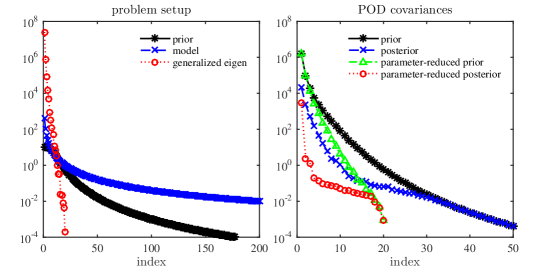
Figure 2: The impact of parameter reference distributions on model reduction, as described in Example 3.6. Left: spectra of the prior covariance matrix $\Gamma_{\rm pr}$ (stars) and the system model $L$ (crosses), along with generalized eigenvalues from (15) (circles). Right: spectra of the state covariance matrices induced by the prior, the posterior, the parameter-reduced prior, and the parameter-reduced posterior; these are denoted by stars, crosses, triangles and circles, respectively.

Table 2: Summary of state reduction methods: the associated state covariance matrix, whether the process is offline/online, and whether adaptive sampling is required.

Method	state covariance	online/offline	adaptive sampling?
Posterior-LISS	$\widetilde{K}_{\rm post}=\int_{\mathbb{X}}u(\Phi_{r}x_{r})u(\Phi_{r}x_{r})^{\top}\pi(dx_{r}|y_{\rm obs})$	online	yes
Laplace-LISS	$\widetilde{K}_{\rm L}\;\;\;=\int_{\mathbb{X}}u(\Pi_{r}x)u(\Pi_{r}x)^{\top}\pi_{\rm L}(dx)$	online	no
Prior-POD	$\widetilde{K}_{\rm pr}\;\;=\int_{\mathbb{X}}u(\Phi_{r}x_{r})u(\Phi_{r}x_{r})^{\top}\pi_{0}(dx_{r})$	offline	no

Since the amount of state variation in the reduced parameter subspace is greatly reduced relative to that induced by either the full-dimensional posterior or the full-dimensional prior, we will henceforth construct reduced-order models only within the reduced parameter subspace. For each state reduction technique of this kind, Table 2 summarizes the specific form of the state covariance, whether reduction is offline/online, and whether adaptive sampling is required, given the choice of parameter reference distribution. Overall, the benefit of pursuing model reduction on the reduced parameter subspace is twofold: first, this approach addresses challenges in the scalability of model reduction with parameter dimension; second, it reduces the computational cost of handling high-dimensional parameters in the parameterized reduced model.

3.2.3 Jointly-approximated posterior

By replacing the forward model $F:{}^{n}\rightarrow{}^{d}$ with the reduced-order model $\tilde{F}:{}^{r}\rightarrow{}^{d}$, the data-misfit function (4) can be approximated as

$$\tilde{\eta}(x_{r})=\frac{1}{2}\|\tilde{F}(x_{r})-y_{\rm obs}\|^{2}_{\Gamma_{\rm obs}}.$$ (28)

Then the resulting jointly-reduced posterior distribution has the form

$$\tilde{\pi}(x_{r}|y_{\rm obs})\propto\exp\left(-\tilde{\eta}(x_{r})\right)\pi_{0}(x_{r}).$$ (29)

Together with the complement prior, this defines a product-form jointly-approximated posterior

$$\tilde{\pi}(x|y_{\rm obs})\propto\tilde{\pi}(x_{r},x_{\perp}|y_{\rm obs})\propto\tilde{\pi}(x_{r}|y_{\rm obs})\pi_{0}(x_{\perp}).$$ (30)

We use the descriptor ‘joint’ to signify that both the parameter space and the model state space have been reduced in these posterior approximations. Because the high-dimensional complement prior $\pi_{0}(x_{\perp})$ is analytically tractable and the low-dimensional jointly-reduced posterior avoids computationally expensive full forward model evaluations, this jointly-approximated posterior can be used to design scalable and computationally efficient posterior exploration schemes.

Remark 3.7 (Data reduction).

In problems where the data set is high-dimensional, the computation time required to evaluate the data-misfit function (4) can also be significant. These evaluations can be accelerated by exploiting low-dimensional structure in the data space, via the DEIM method. Suppose that the dimension of the output of the observation model, $y=C(V_{s}u_{s},\Phi_{r}x_{r})$, is much larger than the reduced parameter dimension and the reduced state dimension. Suppose also that the variation of the model outputs, $C(V_{s}u_{s},\Phi_{r}x_{r})$, can be captured by a subspace spanned by a basis $Y_{o}\in{}^{d\times o}$ that is orthogonal with respect to $\langle\cdot,\cdot\rangle_{\Gamma_{\rm obs}}$. As in the model reduction case, the DEIM method can be used to identify a masking matrix $P_{o}=[\delta_{p_{1}},\ldots,\delta_{p_{o}}]$, where $\delta_{i}$ is the canonical basis in ^o, such that $P_{o}^{\top}Y_{o}$ is nonsingular. Thus we can determine a low-dimensional coefficient function

$$\beta(u_{s},x_{r})=\left(P_{o}^{\top}Y_{o}\right)^{-1}P_{o}^{\top}\,C(V_{s}u_{s},\Phi_{r}x_{r}),$$ (31)

which selectively evaluates the nonlinear function $C$ at indices $p_{1},\ldots,p_{o}$. The resulting approximated observation model has the form

$$\tilde{y}=Y_{o}\,\beta(u_{s},x_{r}).$$ (32)

In this setting, the coefficient function $\beta$ and the reduced system model (20) together define a new reduced-order forward model $\hat{F}:{}^{r}\rightarrow{}^{o}$ that has a smaller number of outputs. This corresponds to model outputs $\tilde{y}=Y_{o}\hat{F}(x_{r})$ in the original observable space. It leads to an approximated data-misfit function in the form of

$$\tilde{\eta}(x_{r}) =\frac{1}{2}\left\|Y_{o}\hat{F}(x_{r})-y_{\rm obs}\right\|^{2}_{\Gamma_{\rm obs}}$$

$$=\frac{1}{2}\left\|\hat{F}(x_{r})-Y_{o}^{\top}\Gamma_{\rm obs}^{-1}\,y_{\rm obs}\right\|^{2}+c,$$ (33)

where $c=\frac{1}{2}\|(I-Y_{o}Y_{o}^{\top})\,y_{\rm obs}\|^{2}_{\Gamma_{\rm obs}}$ is a constant. As in the state reduction case, we can also use a POD approach with the parameter-reduced posterior, the Laplace approximation, or the parameter-reduced prior as reference distributions for constructing the reduced data basis.

3.3 Integrated algorithms

Concisely, construction of the jointly-approximated posterior distribution involves parameter reduction followed by model reduction. Combining the parameter reduction methods of Section 3.1 with the state reduction methods of Section 3.2 leads to various integrated strategies for this task. We list several algorithmic options in Table 3, distinguished according to their online/offline nature and whether adaptive sampling is required.

Table 3: Summary of sampling strategies for constructing the jointly-approximated posterior.

Strategy	Prior-KL-POD	Prior-Joint	Laplace-Joint	Posterior-Joint
Parameter reduction	Prior-KL	Prior-LIPS	Laplace-LIPS	Posterior-LIPS
State reduction	Prior-POD	Prior-POD	Laplace-LISS	Posterior-LISS
Sampling requirement	offline	offline	online	online and adaptive

3.3.1 Non-iterative strategies

The Prior-KL-POD strategy is the simplest option above: we compute the reduced parameter basis using the truncated KL expansion of the prior, and then compute a POD basis for the state by sampling from the parameter-reduced prior. In contrast, the Prior-Joint strategy uses the prior expectation of the GNH to construct a low-dimensional parameter subspace and defines the parameter-reduced prior accordingly; this strategy is still entirely offline, as both the parameter and state subspaces are independent of the data. Only prior samples are required in these two strategies. Full model evaluations in the Prior-POD step and Hessian evaluations in Prior-LIPS estimation can be massively parallelized. The computational cost of Prior-KL-POD is less than that of Prior-Joint, since the former involves no Hessians in the parameter reduction step.

Given observed data, the Laplace-Joint strategy involves first finding the posterior mode by solving an optimization problem. Then samples can be directly drawn from the Laplace approximation (12). In this way, the GNH evaluations required for Laplace-LIPS parameter reduction and the full model evaluations required for Laplace-LISS state reduction can also be carried out in parallel. The computational cost thus is comparable to that of the Prior-Joint strategy. However, in contrast with Prior-Joint, Laplace-Joint is an online strategy that depends on a particular realization of the observed data—and on the associated approximation of the posterior. Using the data focuses attention on regions of high posterior probability and leads to a localization effect in the identification of subspaces; thus, we expect that the jointly-approximated posterior computed by Laplace-Joint will have better accuracy than those produced by the Prior-KL-POD or Prior-Joint strategies, for comparable dimensions of the parameter and state bases. We will explore this conjecture in numerical results below.

3.3.2 Iterative strategy

In the Posterior-Joint strategy, constructing parameter and state subspaces requires computing expectations over the full posterior (to obtain the posterior-LIPS) and the parameter-reduced posterior (to obtain the posterior-LISS). Since direct sampling is not feasible a priori—after all, we are computing these bases in order to facilitate posterior sampling—Algorithm 1 proposes an iterative sampling framework to construct the reduced bases adaptively during posterior exploration.

1:At iteration $k=0$, initialize the jointly-approximated posterior $\tilde{\pi}^{0}(x|y_{\rm obs})$ to be either the prior or the Laplace approximation (12).

2:At iteration $k$, given (i) the reduced data-misfit function $\tilde{\eta}^{k}(x_{r})$ and the jointly-reduced posterior $\tilde{\pi}^{k}(x_{r}|y_{\rm obs})$ induced by the LIPS basis $\Phi_{r}^{k}$ and the LISS basis $V_{s}^{k}$; (ii) the projector $\Pi_{r}^{k}=\Phi_{r}^{k}(\Xi_{r}^{k})^{\top}$ as in Definition 3.1; and (iii) the resulting jointly-approximated posterior $\tilde{\pi}^{k}(x|y_{\rm obs})$, one iteration of the algorithm is:

3:if $k=0$ then

4:     Generate two sample sets, $\{x_{i}\}_{i=1}^{N}$ and $\{x_{i}\}_{i=1}^{M}$, from $\tilde{\pi}^{0}(x|y_{\rm obs})$ by direct sampling.

5:else

6:     Generate two sample sets, $\{x_{i}\}_{i=1}^{N}$ and $\{x_{i}\}_{i=1}^{M}$, from $\tilde{\pi}^{k}(x|y_{\rm obs})$ by applying MCMC to $\tilde{\pi}^{k}(x_{r}|y_{\rm obs})$ and direct sampling to $\pi_{0}(x_{\perp})$.

7:end if

8:Compute the LIPS basis $\Phi_{r}^{k+1}$ by finding the dominant eigenvectors of $(\widehat{S}_{\rm post},\Gamma_{\rm pr}^{-1})$, where

$$\widehat{S}_{\rm post}=\frac{1}{\sum_{i=1}^{N}\omega_{i}}\sum_{i=1}^{N}\omega_{i}\,H(x_{i}),\ \ \text{and}\ \ \omega_{i}=\exp\left(\tilde{\eta}^{k}\left((\Xi_{r}^{k})^{\top}x_{i}\right)-\eta(x_{i})\right).$$ (34)

9:Update the projector $\Pi_{r}^{k+1}=\Phi_{r}^{k+1}(\Xi_{r}^{k+1})^{\top}$ and compute the weighted snapshot matrix

$$U=\frac{1}{\sqrt{\sum_{i=1}^{M}\upsilon_{i}}}\left[\sqrt{\upsilon_{1}}u\left(\Pi_{r}^{k+1}x_{1}\right),\ldots,\sqrt{\upsilon_{M}}u\left(\Pi_{r}^{k+1}x_{M}\right)\right],$$ (35)

where $\upsilon_{i}=\exp\left(\tilde{\eta}^{k}\left((\Xi_{r}^{k})^{\top}x_{i}\right)-\eta\left((\Xi_{r}^{k+1})^{\top}x_{i}\right)\right)$, and then compute the reduced state basis $V_{s}^{k+1}$ via the SVD of $U$.

10:For system models involving nonlinear functions, compute the DEIM basis $\Theta_{t}^{k+1}$ as in Step 7, and then construct the masking matrix $P_{t}^{k+1}$.

11:Update $\tilde{\eta}^{k+1}(x_{r})$, $\tilde{\pi}^{k+1}(x_{r}|y_{\rm obs})$ and $\tilde{\pi}^{k+1}(x|y_{\rm obs})$.

12:At $k=0$, importance sampling is turned off, i.e., $\omega_{i}=1$ and $\upsilon_{i}=1$.

Algorithm 1 Iterative construction used in the Posterior-Joint strategy.

In Algorithm 1, we initialize the jointly-approximated posterior to be either the prior or the Laplace approximation (12). At each iteration $k$, two independent sets of samples are generated from the current jointly-approximated posterior, $\tilde{\pi}^{k}(x|y_{\rm obs})$, in order to construct reduced parameter and state bases using the Posterior-LIPS and Posterior-LISS methods, respectively. In this step, samples can be directly drawn when $k=0$. For $k>0$, sampling $\tilde{\pi}^{k}(x|y_{\rm obs})$ requires applying MCMC to the low-dimensional and cheap-to-evaluate jointly-reduced posterior $\tilde{\pi}^{k}(x_{r}|y_{\rm obs})$, and directly sampling the high-dimensional complement prior $\pi_{0}(x_{\perp})$. At each iteration $k$, we use the current jointly-approximated posterior $\tilde{\pi}^{k}(x|y_{\rm obs})$ as the biasing distribution to compute the posterior expectation of the GNH via importance sampling; this process can be written as

$$S_{\rm post}=\int_{\mathbb{X}}\frac{\pi(x|y_{\rm obs})}{\tilde{\pi}^{k}(x|y_{\rm obs})}\,H(x)\,\tilde{\pi}^{k}(dx|y_{\rm obs}).$$ (36)

Given the data-misfit function $\tilde{\eta}^{k}(x_{r})$ induced by the current reduced order model, the importance weight

$$\frac{\pi(x|y_{\rm obs})}{\tilde{\pi}^{k}(x|y_{\rm obs})}\propto\omega(x):=\exp\left(\tilde{\eta}^{k}(x_{r})-\eta(x)\right),\;\;{\rm where}\;\;x_{r}=(\Xi_{r}^{k})^{\top}x,$$ (37)

can only be computed up to a normalizing constant. This leads to the self-normalized importance sampling estimator of $\widehat{S}_{\rm post}$ in (34). By finding the dominant eigenvectors of the pencil $(\widehat{S}_{\rm post},\Gamma_{\rm pr}^{-1})$, we obtain the new LIPS basis $\Phi_{r}^{k+1}$.

Remark 3.8.

We note that it is not feasible to store and factorize the matrix $\widehat{S}_{\rm post}$ directly. By computing the action of the local GNH $H(x_{i})$ on vectors—each action requires one forward model evaluation and one adjoint model evaluation—low-rank approximations of each sampled $H(x_{i})$ can be computed using Krylov subspace methods [45] or randomized algorithms [46, 47]. Monte Carlo estimates of the expected Hessians used to identify the Laplace-LIPS and the Prior-LIPS are constructed in the same way. We refer readers to [15, 17] for more details on storage management and computational strategies.

The updated LIPS basis $\Phi_{r}^{k+1}$ leads to a new parameter-reduced posterior $\pi^{k+1}(x_{r}|y_{\rm obs})$, and then the next task is to compute the new reduced-order model using the Posterior-LISS. Since finding the Posterior-LISS requires integration over $\pi^{k+1}(x_{r}|y_{\rm obs})$, which can be computationally expensive, we again employ importance sampling with the previous jointly-approximated posterior $\tilde{\pi}^{k}(x|y_{\rm obs})$ as the biasing distribution. We use the following identity

$$\widetilde{K}_{\rm post} =\int_{\mathbb{X}_{r}}u\left(\Phi_{r}^{k+1}x_{r}\right)u\left(\Phi_{r}^{k+1}x_{r}\right)^{\top}\pi^{k+1}(dx_{r}|y_{\rm obs}),$$

$$=\int_{\mathbb{X}}u\left(\Pi_{r}^{k+1}x\right)u\left(\Pi_{r}^{k+1}x\right)^{\top}\hat{\pi}^{k+1}(dx|y_{\rm obs}),$$

to derive the importance sampling formula in the full parameter space. Thus, the state covariance estimated over $\pi^{k+1}(x_{r}|y_{\rm obs})$ can be written as

$$\widetilde{K}_{\rm post}=\int_{\mathbb{X}}\frac{\hat{\pi}^{k+1}(x|y_{\rm obs})}{\tilde{\pi}^{k}(x|y_{\rm obs})}\,u\left(\Pi_{r}^{k+1}x\right)u\left(\Pi_{r}^{k+1}x\right)^{\top}\,\tilde{\pi}^{k}(dx|y_{\rm obs}).$$ (38)

As in the parameter reduction case, the likelihood ratio

$$\frac{\hat{\pi}^{k+1}(x|y_{\rm obs})}{\tilde{\pi}^{k}(x|y_{\rm obs})}\propto\upsilon(x):=\exp\left(\tilde{\eta}^{k}\left((\Xi_{r}^{k})^{\top}x\right)-\eta\left((\Xi_{r}^{k+1})^{\top}x\right)\right),$$ (39)

can only be computed up to a normalizing constant, and therefore we use self-normalized importance sampling. When the SVD is used to compute the POD basis, this leads to the weighted snapshot matrix in (35). We note that the full model evaluation in the parameter-reduced data-misfit function $\eta\left((\Xi_{r}^{k+1})^{\top}x\right)$ in (39) generates exactly the snapshot $u(\Pi_{r}^{k+1}x)$ used in computing the POD basis.

At the first iteration, the initial distribution $\tilde{\pi}^{0}(x|y_{\rm obs})$ can have a large discrepancy from the posterior, and thus the resulting importance weights $\omega_{i}$ and $\upsilon_{i}$ can potentially have large variances. To overcome this potential sampling deficiency, we set the weights $\omega_{i}$ and $\upsilon_{i}$ to $1$ at the first iteration. This way, the initial distribution is used as a surrogate to explore the support of the posterior, and importance sampling only kicks in at later iterations to estimate the LIPS and the LISS.

Remark 3.9.

In each iteration of Algorithm 1, constructing the LIPS involves evaluating the forward model—and hence the full posterior density—at a set of samples, and computing the action of the GNH on a number of directions for each sample in this set. In addition, the forward model and the full posterior density are evaluated at another set of samples—projected onto the subspace spanned by the LIPS—to construct the reduced-order model. Based on our numerical experience, a sample size on the order of hundreds is sufficient for both steps. We also note that the first iteration of Algorithm 1 generates a jointly-approximated posterior equivalent to the result of either the Prior-Joint strategy or the Laplace-Joint strategy, depending on the choice of initial distribution.

To ensure the convergence of the self-normalized importance sampling estimators (34) and (35), it is required that $\tilde{\pi}^{k}(x|y_{\rm obs})>0$ whenever $\pi(x|y_{\rm obs})>0$ , and that $\tilde{\pi}^{k}(x|y_{\rm obs})>0$ whenever $\hat{\pi}^{k+1}(x|y_{\rm obs})>0$, for any $k>0$. Furthermore, distributions constructed from the low-dimensional subspaces are not guaranteed to capture the tails of the posterior accurately, and hence the weights $\omega(x)$ and $\upsilon(x)$ might have large variance in some situations. Bounding $\omega(x)$ and $\upsilon(x)$ from above, however, can control the variance of the importance weights and thus guarantee finite variance of the estimators. The following lemma establishes that by assigning upper bounds to the approximated data-misfit functions, the ratios $\omega(x)$ and $\upsilon(x)$ can be bounded.

Lemma 3.10.

Given an upper bound $K>0$ on the parameter-approximated data-misfit function $\eta(\Xi_{r}^{\top}x)$ and the jointly-approximated data-misfit function $\tilde{\eta}(\Xi_{r}^{\top}x)$, i.e.,

$$\eta(\Xi_{r}^{\top}x)\leq K<\infty\;\;{\rm and}\;\;\tilde{\eta}(\Xi_{r}^{\top}x)\leq K<\infty,$$ (40)

the ratios $\omega(x)$ and $\upsilon(x)$ defined in (36) and (39) are bounded as $\omega(x)\leq\exp(K)$ and $\upsilon(x)\leq\exp(K)$.

Proof.

Since all the data-misfit functions have the form of a weighted $L^{2}$ norm, their values cannot be negative, i.e., $\eta\left(x\right)\geq 0$, $\eta(\Xi_{r}^{\top}x)\geq 0$, and $\tilde{\eta}(\Xi_{r}^{\top}x)\geq 0$. The upper bounds on $\eta(\Xi_{r}^{\top}x)$ and $\tilde{\eta}(\Xi_{r}^{\top}x)$ in (40) then lead to

$$\tilde{\eta}(x_{r})-\eta(x)\leq K\;\;{\rm and}\;\;\tilde{\eta}(\Xi_{r}^{\top}x)-\eta(\Xi_{r}^{\top}x)\leq K.$$

Thus both ratios $\omega(x)$ and $\upsilon(x)$ are bounded above by $\exp(K)$. ∎

We employ a heuristic based on a (somewhat frequentist) probabilistic argument to choose a value of $K$ to impose as a bound on our misfit functions. If the whitened residual in the data-misfit function, $\Gamma_{\rm obs}^{-1/2}(F(x)-y_{\rm obs})$, is a $d$-dimensional random vector whose components are independent standard Gaussians, then the data-misfit function follows a chi-squared distribution with $d$ degrees of freedom, $\chi_{d}^{2}$. Then the upper bound $K$ can be chosen so that the probability of the data-misfit function exceeding $K$ is $\tau_{d}\ll 1$, i.e.,

$${\mathbb{P}}[z>K]=\tau_{d},\ \ \text{where}\ \ z\sim\chi_{d}^{2}.$$

Here we choose $\tau_{d}=10^{-4}$.

3.3.3 Posterior exploration schemes

The jointly-approximated posterior provides a launching point for many scalable and computationally efficient posterior sampling schemes: the analytically tractable and high-dimensional complement prior is sampled directly, while the low-dimensional and analytically intractable jointly-reduced posterior can be sampled by various MCMC methods. Evaluations of the latter density are accelerated because they rely only on the reduced-order forward model. In this paper, we employ the adaptive Metropolis-adjusted Langevin Algorithm (MALA) [48] to sample the jointly-reduced posterior. We note that the separable representation of the jointly-approximated posterior is amenable to a range of alternative posterior exploration or integration approaches, e.g., implicit sampling [49, 50], the randomize-then-optimize method [51], and sparse quadrature [52, 53, 54].

If, on the other hand, one would like to compute the expectation of a function of interest $g(x)$ over the full posterior, samples from the jointly-approximated posterior can be used to derive importance sampling estimates thereof. Bounding the jointly-approximated posterior as in Lemma 3.10, and using the identity

$$\mathbb{E}\left[g(x)\right]=\int_{\mathbb{X}}g(x)\,\pi(dx|y_{\rm obs})=\int_{\mathbb{X}}\frac{\pi(x|y_{\rm obs})}{\tilde{\pi}(x|y_{\rm obs})}\,g(x)\,\tilde{\pi}(dx|y_{\rm obs}),$$

yields the estimator

$$\mathbb{E}\left[g(x)\right]\approx\frac{1}{\sum_{i=1}^{N}\omega(x_{i})}\sum_{i=1}^{N}\omega(x_{i})g(x_{i}),$$ (41)

where $\omega(x)=\exp\left(\tilde{\eta}\left(\Xi_{r}^{\top}x\right)-\eta\left(x\right)\right)$ and $x_{i}\sim\tilde{\pi}(x|y_{\rm obs})$ for $i=1,\ldots,N$. This ratio $\omega(x)$ could also be used in a delayed-acceptance MCMC method [22, 23] to sample the full posterior; in this case, the jointly-approximated posterior is used to “screen” MCMC proposals and thus more quickly traverse the support of the full posterior. Note that the importance sampling estimator above requires a full posterior evaluation to compute each importance weight. This effort can be computationally demanding, but these full posterior evaluations can be massively parallelized, as the sampling step is based on the jointly-approximated posterior. Further variance reduction might be achieved using the control variates technique [55].

4 Example 1: atmospheric remote sensing

In this section, we apply our joint approximation approach to a realistic atmospheric remote sensing problem, where satellite observations from the Global Ozone MOnitoring System (GOMOS) are used to estimate the concentration profiles of various gases in the atmosphere. We will first present the GOMOS model, the inverse problem setup, and the reduced-order model. Then we will demonstrate various aspects of the joint posterior approximation using the GOMOS inversion.

4.1 Problem setup

The GOMOS instrument repeatedly measures light intensities $\rho_{\nu}$ at different wavelengths $\nu$. First, a reference intensity spectrum $\rho_{\rm ref}$ is measured above the atmosphere. The transmission spectrum is defined as $T_{\nu}=\rho_{\nu}/\rho_{\rm ref}$. The transmissions measured at wavelength $\nu$ along the ray path $z$ are modelled using Beer’s law:

$$T_{\nu,z}=\exp\left(-\int_{z}\sum_{\mathrm{gas}}a_{\nu}^{\mathrm{gas}}(z(\zeta))\kappa^{\mathrm{gas}}(z(\zeta))d\zeta\right),$$ (42)

where $\kappa^{\mathrm{gas}}(z(\zeta))$ is the density of a gas (unknown parameter) at tangential height $z$. The so-called cross-sections $a_{\nu}^{\mathrm{gas}}$, known from laboratory measurements, define how much a gas absorbs light at a given wavelength.

To approximate the integrals in (42), the atmosphere is discretized. The geometry used for inversion resembles an onion: the gas densities are assumed to be constant within spherical layers around the Earth. The GOMOS measurement principle is illustrated in Figure 3.

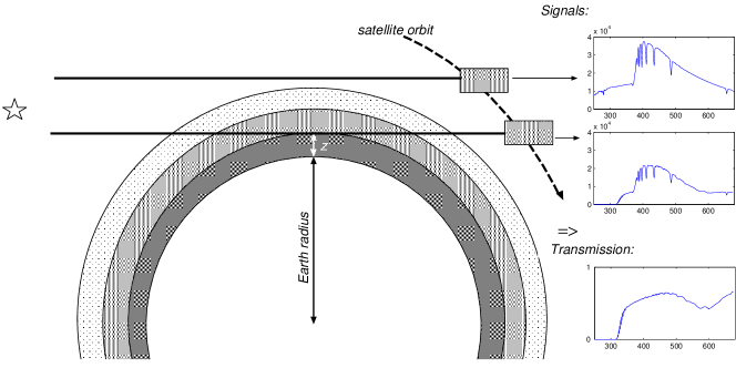
Figure 3: The principle of the GOMOS measurement. The reference intensity is measured above the atmosphere. The observed transmission spectrum is the attenuated spectrum (measured through the atmosphere) divided by the reference spectrum. The atmosphere is presented locally as spherical layers around the Earth. Note that the thickness of the layers is much larger relative to the Earth in this figure than in reality. The figure is adopted from [56], with the permission of the authors.

We assume that the cross-sections do not depend on height. In the inverse problem we have $N_{\rm gas}$ gases, $N_{\nu}$ wavelengths, and the atmosphere is divided into $N_{\rm alts}$ layers. The discretization is fixed so that number of measurement lines is equal to the number of layers. Approximating the integrals by sums over the chosen grid, and combining information from all lines and all wavelengths, we can write the model in matrix form as follows:

$$T=\exp(-AB^{\top}G^{\top}),$$

where $T\in{}^{N_{\nu}\times N_{\rm alts}}$ are the modelled transmissions, $A\in{}^{N_{\nu}\times N_{\rm gas}}$ contains the cross-sections, $B\in{}^{N_{\rm alts}\times N_{\rm gas}}$ contains the unknown densities, and $G\in{}^{N_{\rm alts}\times N_{\rm alts}}$ is the geometry matrix that contains the lengths of the lines of sight in each layer.

Each gas density profile is endowed with an independent log-normal process prior. Equivalently, the gas density profiles can be represented as $B=\exp(X)$. Using MATLAB notation, each discretized log-profile $X(:,i)$ follows a Gaussian prior $N(\mu_{\rm pr}^{(i)},\Gamma_{\rm pr}^{(i)})$, where $\Gamma_{\rm pr}^{(i)}$ is defined by the squared exponential covariance kernel

$$C_{i}(\zeta,\zeta^{\prime})=\sigma_{i}\exp\left(-\frac{\|\zeta-\zeta^{\prime}\|^{2}}{2\zeta_{0}^{2}}\right),$$ (43)

where the correlation length is $\zeta_{0}=10$. In the example below, we will infer $N_{\rm gas}=4$ unknown gas profiles; thus we choose $\sigma_{1}=5.22$, $\sigma_{2}=9.79$, $\sigma_{3}=23.66$, and $\sigma_{4}=83.18$. These priors are chosen to promote smooth gas density profiles with large variations.

Now let $\otimes$ denote the Kronecker product and $\mathrm{vec}(\cdot)$ be a vectorization operator that stacks the columns of its matrix argument on top of each other. Using the identity $\mathrm{vec}(AB^{\top}G^{\top})=(G\otimes A)\mathrm{vec}(B^{\top})$, we obtain the vectorized parameter-to-data relationship,

$$y_{\rm obs}=\mathrm{vec}(T)+e=\exp\left(-(G\otimes A)\exp(x)\right)+e,$$ (44)

where $x=\mathrm{vec}(X^{\top})$ are the vectorized parameters and $e$ is the measurement error modeled by independent Gaussian random variables with known variances. Here we adopt the same model setup and synthetic data set used in [15]. The atmosphere is discretized into $N_{\rm alts}=50$ layers, and with four profiles to infer, the total dimension of the parameter is $n=200$. We have observations at $N_{\nu}=1416$ wavelengths, and thus the dimension of the data is $d=70800$. Although the data dimension is much higher than the parameter dimension in this case, the resulting inverse problem is still ill-posed. The forward model introduces a strong smoothing effect, and thus the high-dimensional data can inform only a small number of parameter dimensions. Similar situations are encountered in X-ray tomography [14], where the forward model also involves a system of integral equations. We refer the readers to [15] for a further description of the model setup and the data set. For more details about the GOMOS instrument and the Bayesian treatment of the inverse problem, see [56, 57] and the references therein.

The forward model $y=\exp\left(-(G\otimes A)\exp(x)\right)$ maps from ²⁰⁰ to ⁷⁰⁸⁰⁰ and involves two exponential functions. Given a reduced parameter basis $\Phi_{r}$ and a realization of the reduced parameter $x_{r}$, the computational expense of evaluating the forward model with the reduced parameter, $\exp\left(-(G\otimes A)\exp(\Phi_{r}x_{r})\right)$, arises from several sources: the exponential expression $\exp(\Phi_{r}x_{r})$, which involves a matrix-vector product and a $200$-dimensional exponential function evaluation; the matrix-vector product with $G\otimes A$; and the evaluation of the $70800$ dimensional exponential function for producing the model outputs. To set up the reduced-order model, the first task is to construct a DEIM interpolation for the exponential function $\exp(\Phi_{r}x_{r})$. Given a basis $\Theta_{t}$ that spans the subspace capturing the variations of the outputs of $\exp(\Phi_{r}x_{r})$ and the associated masking matrix $P_{t}$, this DEIM interpolation takes the form

$$\exp(\Phi_{r}x_{r})\approx\Theta_{t}\alpha(x_{r}),\quad{\rm where}\quad\alpha(x_{r})=(P_{t}^{\top}\Theta_{t})^{-1}\exp(P_{t}^{\top}\Phi_{r}x_{r}).$$

Then, given a reduced data basis $Y_{o}$ and the associated masking matrix $P_{o}$, another DEIM interpolation is employed to reduce the output dimension of the forward model in the form of

$$\tilde{F}(x_{r})=(P_{o}^{\top}Y_{o})^{-1}\exp\left(-P_{o}^{\top}(G\otimes A)\Theta_{t}\alpha(x_{r})\right).$$ (45)

In the reduced-order model above, the computational cost is dominated by the evaluation of the nonlinear function $\alpha:{}^{r}\rightarrow{}^{t}$, the matrix-vector product with the $o\times t$ dimensional matrix $P_{o}^{\top}(G\otimes A)\Theta_{t}$, and the $o$-dimensional exponential function. The reduced-order model (45) is used together with the approximated data-misfit function (33) to accelerate evaluations of the original data-misfit function, which involved high-dimensional model outputs.

4.2 Numerical results

We first benchmark the parameter reduction methods introduced in Section 3.1. The (squared) Hellinger distance between the full posterior $\pi(x|y_{\rm obs})$ and the parameter-approximated posterior $\hat{\pi}(x|y_{\rm obs})$,

$$D_{\rm H}^{2}\left(\pi(x),\hat{\pi}(x)\right)=\frac{1}{2}\int_{\mathbb{X}}\left(\sqrt{\pi(x|y_{\rm obs})}-\sqrt{\hat{\pi}(x|y_{\rm obs})}\right)^{2}dx,$$ (46)

is used to evaluate the errors induced by various parameter reduction methods, and to examine convergence versus the number of basis vectors used for the parameter subspace (LIPS or Prior-KL). Results are shown in Figure 4. In this example, all three likelihood-informed methods converge more quickly than Prior-KL (triangles). As expected, Prior-LIPS (squares) is outperformed by the other two likelihood-informed methods, and Posterior-LIPS (crosses) is more accurate than the other methods for any given parameter subspace dimension. We note that the Laplace approximation itself (dashed line) has a rather large Hellinger distance from the posterior. This reflects the non-Gaussianity of the problem, and should not be confused with the fact that the convergence curve of the non-Gaussian Laplace-LIPS approximation (diamonds) is sandwiched between those of Prior-LIPS and Posterior-LIPS.

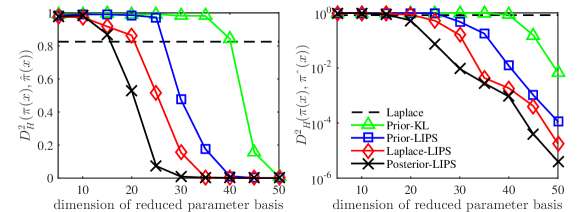
Figure 4: Convergence of various parameter reduction methods, for the GOMOS example: squared Hellinger distances (46) versus the dimensions of the reduced parameter bases $\Phi_{r}$ defined by Posterior-LIPS, Laplace-LIPS, Prior-LIPS, and Prior-KL. The dashed line represents the squared Hellinger distance between the full posterior and its Laplace approximation (12). Both subfigures show the same data, but for clarity we plot with both linear (right) and semilog (left) scales.

Given a $28$-dimensional parameter basis built by Posterior-LIPS, we next benchmark the state reduction methods introduced in Section 3.2. The (squared) Hellinger distance between the parameter-reduced posterior $\pi(x_{r}|y_{\rm obs})$ and the jointly-reduced posterior $\tilde{\pi}(x_{r}|y_{\rm obs})$,

$$D_{\rm H}^{2}\left(\pi(x_{r}),\tilde{\pi}(x_{r})\right)=\frac{1}{2}\int_{\mathbb{X}_{r}}\left(\sqrt{\pi(x_{r}|y_{\rm obs})}-\sqrt{\tilde{\pi}(x_{r}|y_{\rm obs})}\right)^{2}dx_{r},$$ (47)

is used to compare the convergence of various state reduction methods, as a function of the number data basis vectors used in the approximated data-misfit function (33). Four DEIM approximations of the exponential function $\exp(\Phi_{r}x_{r})$, with reduced bases $\Theta_{t}$ of dimension $20$, $40$, $60$ and $80$, are used in this benchmark. Results are shown in Figure 5. In this test, Prior-POD fails to produce a jointly-reduced posterior of reasonable accuracy (we observe $D_{\rm H}^{2}\left(\pi(x_{x}),\tilde{\pi}(x_{r})\right)$ always above 0.9), and thus its performance is not reported. For both Posterior-LISS and Laplace-LISS, the convergence of the resulting jointly-reduced posteriors depends on both the DEIM interpolation of the exponential function $\exp(\Phi_{r}x_{r})$ and on the dimension of the reduced data basis. If the first DEIM interpolation is too coarse (e.g., $\operatorname{dim}(\Theta_{t})=20$ or $40$), the error that can be achieved by refining the reduced data basis reaches a plateau. But for any DEIM interpolation, the jointly-reduced posterior induced by Posterior-LISS is about two orders of magnitude more accurate than that produced by Laplace-LISS.

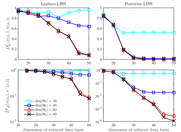
Figure 5: Convergence of various data reduction methods, for the GOMOS example. Squared Hellinger distances (47) versus the dimension of reduced data basis $Y_{o}$ defined by Laplace-LISS and Posterior-LISS are shown in the left and right columns, respectively. Four different DEIM approximations of the exponential function $\exp(\Phi_{r}x_{r})$, with dimensions $20$, $40$, $60$, and $80$, are shown for each case. Again, errors are plotted on linear (top) and logarithmic (bottom) scales.

In the previous comparisons, the posterior-oriented methods (Posterior-LIPS and Posterior-LISS) show clear advantages over the other methods. Thus, we would expect the various strategies for constructing the jointly-approximated posterior in Section 3.3 to have similar performance characteristics. We now demonstrate eight iterations of the Posterior-Joint strategy (Algorithm 1) using either the prior or the Laplace approximation (12) as initial distributions. The reduced parameter bases are truncated at the eigenvalue threshold threshold $\tau_{\rm g}=0.1$, the DEIM basis $\Theta_{t}$ for interpolating the function $\exp(\Phi_{r}x_{r})$ is truncated to retain eigenvalues above $10^{-12}$, and the reduced data basis is truncated to retain eigenvalues above $10^{-5}$. To build the LIPS in each iteration of Posterior-Joint, the forward model and the action of the GNH in multiple directions are evaluated at 200 parameter samples. In particular, for each parameter sample, we use one forward model simulation and the action of GNH on 30 directions. To build the reduced-order model at each iteration, we evaluate the forward model at 500 parameter samples. In comparison, the number of forward model and GNH–action evaluations required by Laplace-Joint or Prior-Joint is exactly the same as that required by one iteration of Posterior-Joint.

To find the MAP, we employ the subspace trust region method of [58, 59] with inexact Newton iterations. Using the prior mean as the initial guess, finding the MAP requires 25 Newton iterations. Each Newton iteration involves one forward model evaluation and the action of the GNH on an average of 8 directions. The computational cost of finding the MAP is much smaller than that of constructing the jointly-approximated posteriors. But we emphasize that sampling the jointly-approximated posteriors does not involve any further full forward simulations.

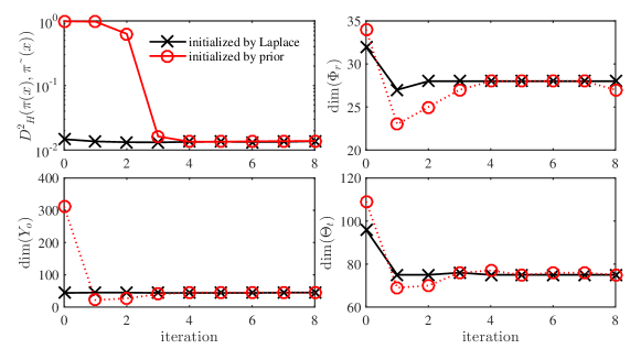
Figure 6: Iterations of Algorithm 1, for the GOMOS example. The logarithm of the squared Hellinger distance (48), and the dimensions of the reduced bases $\Phi_{r}$, $Y_{o}$, and $\Theta_{t}$ are shown. We show iteration histories beginning with two different initial distributions: the prior and the Laplace approximation (12).

As in the previous comparisons, we use the (squared) Hellinger distance between the full posterior $\pi(x|y_{\rm obs})$ and the jointly-approximated posterior $\tilde{\pi}(x|y_{\rm obs})$,

$$D_{\rm H}^{2}\left(\pi(x),\tilde{\pi}(x)\right)=\frac{1}{2}\int_{\mathbb{X}}\left(\sqrt{\pi(x|y_{\rm obs})}-\sqrt{\tilde{\pi}(x|y_{\rm obs})}\right)^{2}dx,$$ (48)

as the error measure. We also compare the dimension of reduced parameter basis $\Phi_{r}$, the dimension of the DEIM basis $\Theta_{t}$, and the dimension of the reduced data basis $Y_{o}$. The results are shown in Figure 6. In this example, when the Laplace approximation is used as the initial distribution, the Hellinger distance (48) remains flat for all iterations, and the dimensions of the various reduced bases stabilize in the first iteration. In contrast, when the prior distribution is used as the initial distribution, the algorithm stabilizes at iteration 4, and the Hellinger distance (48) is rather large in the first three iterations ($>0.9$). We recall that the first iteration of Algorithm 1 generates a jointly-approximated posterior corresponding to either Prior-Joint or Laplace-Joint, depending on the initial distribution. This difference in initial errors also shows that the Laplace-Joint strategy can (by itself) be useful for constructing a jointly-approximate posterior in this case, while the Prior-Joint strategy is not able to provide an accurate approximation.

In Figure 7, we also plot the full posterior and the jointly-approximated posteriors generated by Posterior-Joint (at iteration 8), Laplace-Joint, and Prior-Joint, as well as the Laplace approximation (12), marginalized onto the first eight KL basis functions. Here the full posterior is sampled by the DILI MCMC algorithm of [17], which is an exact sampling method. Both Laplace-Joint and Posterior-Joint yield marginal distributions that are almost identical to those of the full posterior, whereas the marginals of Prior-Joint demonstrate large discrepancies with the full posterior. Overall, for this example, running Laplace-Joint is the most computationally efficient way to generate the jointly-approximated posterior. By running an additional iteration of Posterior-Joint, the dimensions of the reduced bases can be further reduced without loss of accuracy.

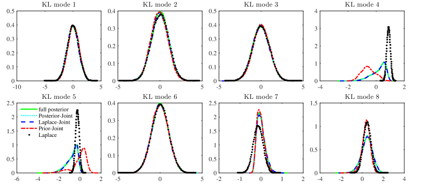
Figure 7: Marginal posterior distributions for the GOMOS example: the full posterior and the jointly-approximated posteriors generated by Posterior-Joint, Laplace-Joint, and Prior-Joint, along with the Laplace approximation (12). We show marginal distributions along each of the first eight KL modes.

5 Example 2: groundwater aquifer inversion

Our second example is an elliptic PDE coefficient inverse problem. In physical terms, our problem setup corresponds to inferring the transmissivity field of a two-dimensional groundwater aquifer from partial observations of the stationary drawdown field of the watertable, measured from well bores.

5.1 Problem setup

Consider a three kilometer by one kilometer problem domain $\Omega=[0\,{\rm m},3000\,{\rm m}]\times[0\,{\rm m},1000\,{\rm m}]$, with boundary $\partial\Omega$. We denote the spatial coordinate by $\zeta\in\Omega$. Consider the transmissivity field $T(\zeta)$ (units [${\rm m}^{2}/{\rm day}$]), the drawdown field $u(\zeta)$ (units [${\rm m}$]), and sink/source terms $q(\zeta)$ (units [${\rm m}/{\rm day}$]). The drawdown field for a given transitivity and source/sink configuration is governed by the elliptic equation:

$$-\nabla\cdot\left(T(\zeta)\nabla u(\zeta)\right)=q(\zeta),\quad\zeta\in\Omega.$$ (49)

We prescribe the drawdown value to be zero on the boundary (i.e., a Dirichlet boundary condition), and define the source/sink term $q(\zeta)$ as the superposition of four weighted Gaussian plumes with standard width $50$ meters. The plumes are centered near the four corners of the domain (at $[20\,{\rm m},20\,{\rm m}]$, $[2980\,{\rm m},20\,{\rm m}]$, $[2980\,{\rm m},980\,{\rm m}]$ and $[20\,{\rm m},980\,{\rm m}]$) with magnitudes of –3000, 2000, 4000, and –300 [${\rm m}/{\rm day}$], respectively. We solve (49) by a finite element method.

The discretized transitivity field $T(\zeta)$ is endowed with a log-normal prior distribution, i.e.,

$$T=\exp(x),\;{\rm and}\;x\sim\mathcal{N}\left(\mu_{\rm pr},\Gamma_{\rm pr}\right),$$ (50)

where the prior mean is set to $\log(1000\,[{\rm m}/{\rm day}])$ and the inverse of the covariance matrix $\Gamma_{\rm pr}^{-1}$ is defined through the discretization of an Laplace-like stochastic partial differential equation [60],

$$(-\nabla\cdot K\nabla+\kappa^{2})x(\zeta)=\mathcal{W}(\zeta),$$ (51)

where $\mathcal{W}(\zeta)$ is white noise. As discussed in [3], this way of defining the precision operator of a Gaussian prior is discretization invariant, i.e., the posterior distribution will converge to its functional limit under grid refinement. In this example, we set the stationary, anisotropic correlation tensor $K$ to

$$K=\left[\begin{array}[]{rr}0.55&-0.45\\ -0.45&0.55\end{array}\right],$$

and put $\kappa=50$. The “true” transmissivity field is a realization from the prior distribution. The true transmissivity field, the sources/sinks, the simulated drawdown field, and the synthetic data are shown in Figure 8. Partial observations of the pressure field are collected at $d=13$ sensors whose locations are depicted by black dots in Figure 8(c). The observation operator $C$ is simply the corresponding “mask” operation. This yields observed data $y_{\rm obs}\in{}^{13}$ as

$$y_{\rm obs}=Cu(\zeta)+e,$$

with additive error $e\sim\mathcal{N}(0,\sigma^{2}I_{13})$. The standard deviation $\sigma$ of the measurement noise is prescribed so that the observations have signal-to-noise ratio $120$, where the signal-to-noise ratio is defined as $\mathbb{V}{\rm ar}(y_{\rm obs})/\sigma^{2}$. The noisy data are shown in Figure 8(d).

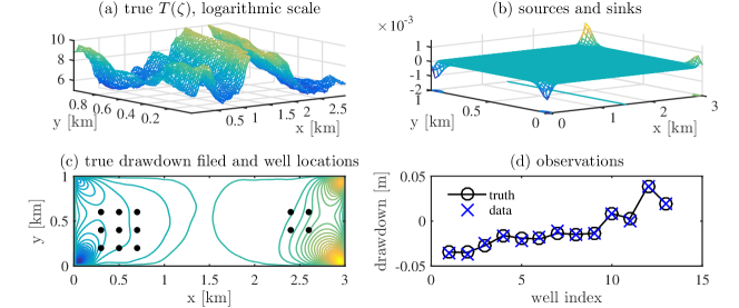
Figure 8: Setup of the groundwater inversion example. (a) “True” transmissivity field. (b) Sources and sinks. (c) Drawdown field resulting from the true transmissivity field, with observation wells indicated by black dots. (d) Data $y_{\rm obs}$; circles represent the noise-free drawdowns at each well, while crosses represent the observed drawdowns corrupted with measurement noise.

In this example, the finite element discretization of (49) uses $120\times 40$ bilinear elements to represent the drawndown field $u(\zeta)$, while the transmissivity field $T(\zeta)$ is modeled as piecewise constant for each element. This yields the discretized system of equations

$$L(T)u=q,\quad T=\exp(x),\quad{\rm and}\quad y=Cu$$ (52)

where the discretized state $u$ has dimension $m=4961$, while the transmissivity field $T$ and parameter $x$ are of dimension $n=4800$. Here, the matrix $L(T)$ can be expressed as

$$L(T)=\sum_{i=1}^{n}L_{i}\exp(x_{i}),$$

where $L_{i}\in{}^{m\times m}$, $i=1,\ldots,n$ are parameter-independent matrices.

Model reduction for (52) consists of two steps. Beginning with a reduced parameter basis $\Phi_{r}$, we first construct a DEIM interpolant for the log-normal process $T\approx\exp(\Phi_{r}x_{r})$. Given a basis $\Theta_{t}$ that spans the subspace capturing variations of $\exp(\Phi_{r}x_{r})$, and the associated masking matrix $P_{t}$, DEIM interpolation takes the form

$$\exp(\Phi_{r}x_{r})\approx\Theta_{t}\alpha(x_{r}),\quad{\rm where}\quad\alpha(x_{r})=(P_{t}^{\top}\Theta_{t})^{-1}\exp(P_{t}^{\top}\Phi_{r}x_{r}).$$

Using MATLAB notation, for a given reduced parameter $x_{r}$, the matrix $L(T)$ can be rewritten as

$$L(T)=\sum_{j=1}^{t}\left(\sum_{i=1}^{n}L_{i}\Theta_{t}(i,j)\right)\alpha_{j}(x_{r}),$$ (53)

where $\alpha_{j}(x_{r})$ is the $j$th component of the vector-valued function $\alpha$. In the second step, given a reduced state basis $V_{s}$, we approximate the state by $u\approx V_{s}u_{s}$ and apply Galerkin projection, yielding a reduced linear system

$$V_{s}^{\top}L(T)V_{s}u_{s}=V_{s}^{\top}q.$$

Substituting (53) into the above equation, the reduced order model can be written as

$$L_{s}(x_{s})u_{s}=q_{s},$$

where

$$L_{s}(x_{s})=\sum_{j=1}^{t}V_{s}^{\top}\left(\sum_{i=1}^{n}L_{i}\Theta_{t}(i,j)\right)V_{s}\alpha_{j}(x_{r})\quad{\rm and}\quad q_{s}=V_{s}^{\top}q,$$

and the associated reduced observation model is $y=(CV_{s})u_{s}$. The computational cost of this reduced order model is dictated by the dimension of the reduced parameter subspace, the reduced state subspace, and the DEIM basis, and is independent of the dimension of the original model.

5.2 Numerical results

We run the same set of tests as in the GOMOS example. The Hellinger distance (46) is used to evaluate the errors induced by various parameter reduction methods, versus the number of basis vectors used in the parameter-approximated posterior. The results are shown in Figure 9. As in the GOMOS example, the Laplace approximation (dashed line) has a rather large Hellinger distance from the posterior. Prior-KL parameter reduction (triangles) converges rather slowly relative to the likelihood-informed methods; it outperforms the Laplace approximation only after 25 or more basis vectors are included. Prior-LIPS (squares) converges more quickly than Prior-KL, but it is outperformed by the other two likelihood-informed methods, which use Hessians at parameter values drawn from approximations of the posterior. The convergence curves of Posterior-LIPS (crosses) and Laplace-LIPS (diamonds) are almost identical.

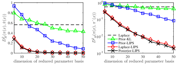
Figure 9: Convergence of various parameter reduction methods, for the elliptic PDE example: squared Hellinger distances (46) versus the dimensions of the reduced parameter bases $\Phi_{r}$ defined by Posterior-LIPS, Laplace-LIPS, Prior-LIPS, and Prior-KL. The dashed line represents the squared Hellinger distance between the full posterior and its Laplace approximation (12).

Given a 17-dimensional likelihood-informed parameter basis built via Posterior-LIPS, we now use the Hellinger distance (47) to evaluate the convergence of various state reduction methods, as a function of the state dimension of the reduced-order model. Because we have a non-smooth prior in this example, a rather high-dimensional DEIM basis is required to ensure positivity in approximating the log-normal process $\exp(\Phi_{r}x_{r})$. Four DEIM approximations of the log-normal process, with reduced bases $\Theta_{t}$ having dimensions $250$, $350$, $450$, and $550$ are used in this benchmark. The results are shown in Figure 10. In this test, Posterior-LISS is about one order of magnitude more accurate than Laplace-LISS, and Laplace-LISS is about one order of magnitude more accurate than Prior-POD. We also note that Posterior-LISS generates the most stable convergence curves among all the methods tested here.

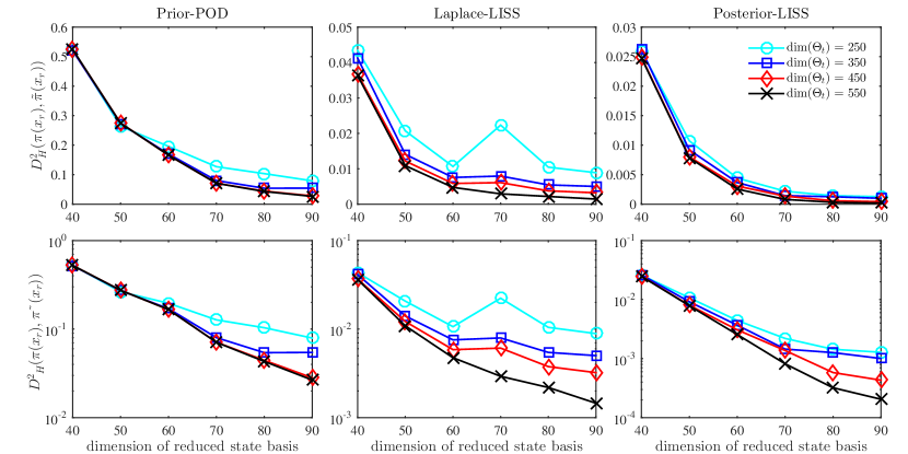
Figure 10: Convergence of various state reduction methods, for the elliptic PDE example. Squared Hellinger distances (47) versus the dimension of reduced state bases $V_{s}$ defined by Prior-POD, Laplace-LISS, and Posterior-LIS are shown in the left, middle, and right columns, respectively. Four different DEIM approximations of the exponential function $\exp(\Phi_{r}x_{r})$, with dimensions $250$, $350$, $450$ and $550$, are shown for each case. Again, errors are plotted with linear (top) and logarithmic (bottom) scales.

We now demonstrate eight iterations of the Posterior-Joint strategy (Algorithm 1) using either the prior or the Laplace approximation (12) as initial distributions. The reduced parameter basis is truncated to retain components above the eigenvalue threshold $\tau_{\rm g}=0.05$, the DEIM basis $\Theta_{t}$ for interpolating the function $\exp(\Phi_{r}x_{r})$ is truncated to retain eigenvalues above $10^{-14}$, and the reduced state basis is truncated to retain eigenvalues above $10^{-6}$. In this example, the numbers of forward model and GNH–action evaluations used in each iteration of Posterior-Joint, or in a full run of Laplace-Joint or Prior-Joint, are the same as those used in the remote sensing example. We note that the action of the GNH in this case can be computed much more quickly than in the remote sensing case: the elliptic PDE forward model is self-adjoint, and hence the solution of the linear system in the forward model can be recycled to compute the action of the GNH without additional linear solves. Using the prior mean as the initial guess, the subspace trust region method requires 21 inexact Newton iterations to find the MAP. Each Newton iteration involves one forward model evaluation and the computation of the GNH action on an average of 5 directions.

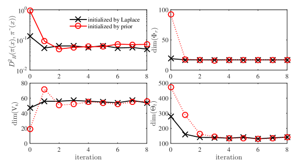
Figure 11: Iterations of Algorithm 1, for the elliptic PDE example. For each iteration, we show the logarithm of the squared Hellinger distance (48), and the dimension of the reduced parameter basis $\Phi_{r}$, the reduced state basis $V_{s}$, and the DEIM basis $\Theta_{t}$. We show iteration histories beginning with two different initial sampling distributions: the prior and the Laplace approximation (12).

As in the GOMOS case, the Hellinger distance (48) from the full posterior is used to evaluate the accuracy of the jointly-approximated posterior. We also show the evolution of the dimension of the reduced parameter basis $\Phi_{r}$, the dimension of the DEIM basis $\Theta_{t}$, and the dimension of the reduced state basis $V_{s}$. Results are shown in Figure 11. In this example, when the Laplace approximation is used to initiate parameter sampling, the Hellinger distance (48) drops slightly at iteration 1, and then stays almost at a constant level for the remaining iterations. The dimensions of various reduced bases also stabilize after the first iteration. When the prior distribution is used to initiate parameter sampling, the algorithm stabilizes at iteration 2, but the Hellinger distance (48) is rather large in the first few iterations ($>0.9$). We recall that the first iteration of Algorithm 1 generates a jointly-approximated posterior from either Prior-Joint or Laplace-Joint, depending on the initial distribution. In Figure 12, we plot the full posterior and the jointly-approximated posteriors generated by Posterior-Joint, Laplace-Joint, and Prior-Joint, as well as the Laplace approximation (12), marginalized onto the first four KL bases. Here the full posterior is sampled by the DILI method of [17]. Both Laplace-Joint and Posterior-Joint have marginal distributions that are almost identical to those of the full posterior, whereas the marginals of Prior-Joint demonstrate significant discrepancies with the full posterior.

Overall, for this example, running Laplace-Joint is the most computationally efficient way to construct the jointly-approximated posterior. Beginning with this approximation and running an additional iteration of Posterior-Joint, the accuracy of the jointly-approximated posterior can be further improved.

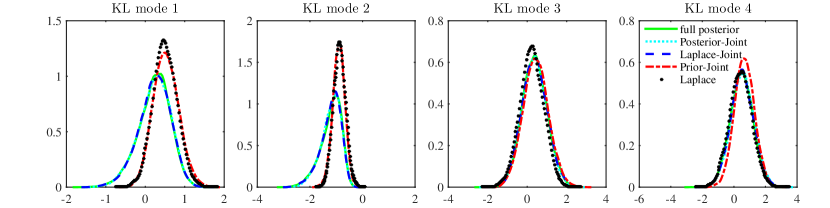
Figure 12: Marginal posterior distributions for the elliptic PDE example: the full posterior and the jointly-approximated posteriors generated by Posterior-Joint, Laplace-Joint, and Prior-Joint, along with the Laplace approximation (12). We show marginal distributions along each of the first four KL modes.

6 Conclusions

This paper addresses two major computational challenges in the Bayesian solution of inverse problems: the high dimensionality of parameters and the large computational cost of forward model evaluations. For many MCMC methods, the cost of sampling scales poorly with the former, while the latter makes repeated evaluations of the posterior density computationally prohibitive. We thus propose a likelihood-informed approach for identifying and exploiting low-dimensional structure in both the parameter space and the model state space. The resulting jointly-approximated posterior can be characterized using only low-dimensional samplers and inexpensive evaluations of a reduced-order model. The computational cost of computing posterior expectations then scales with the dimension of the reduced parameter and state spaces, which reflect the intrinsic complexities of the inverse problem—e.g., how large is the parameter subspace capturing significant changes from prior to posterior, and what variations in the forward model state are induced by the parameter distribution on this subspace.

Previous work on the approximation of Bayesian inverse problems has shown that it is useful to perform some kind of parameter reduction before model reduction [24, 33]. It has also been demonstrated that focusing attention on a particular region of the parameter space—in particular, the region of high posterior probability—enables the construction of more accurate reduced-order models for the purpose of Bayesian inference [16]. The present work uses locality in both of these senses. We reduce parameter dimension by “filtering out” directions of prior variability that are irrelevant to the prior-to-posterior update, i.e., directions that the likelihood does not inform. Within the remaining parameter subspace, we focus on the region of parameter values that is consistent with the data, i.e., that has high posterior probability. Locality in dimension and in parameter range then yields smaller variations in the model state, which are better captured by a reduced-order model. The resulting jointly-approximated posterior can be constructed for systems with high-dimensional parameters and states, and is accurate in the stringent sense of Hellinger distance from the true posterior. As a byproduct of this reduction procedure, we are also able to reduce the cost of handling high-dimensional data, by exploiting low-dimensional structure and sparsity in the data space.

Within this framework, we introduce several alternative strategies for constructing two key building blocks of the posterior approximation: the likelihood-informed parameter subspace (LIPS) and the associated likelihood-informed state subspace (LISS). One interesting aspect of these strategies is the choice of reference distribution; options include the prior, a Laplace approximation of the posterior, or the posterior itself. Our numerical examples demonstrate that posterior-focused reference distributions, while “online” in the sense of depending on the data, yield the most accurate approximations for a given subspace dimension. All of these strategies contain many highly parallelizable computations.

While the present work has used snapshot-style approaches to constructing appropriate subspaces of the parameter space and state space, future work might use optimization on matrix manifolds to directly search for optimal bases in nonlinear settings. It may also be useful to extend beyond the essentially linear dimension reduction strategies employed here to identify nonlinear manifolds that better capture the prior-to-posterior update and associated variations of the model state. Finally, we note that our current approximations focus on inverse problems with nonlinear forward models but prescribed Gaussian priors. It is natural to consider generalizations to hierarchical Gaussian priors, where the prior is not precisely fixed but rather its mean and precision/covariance are controlled by additional hyperparameters. The posterior approximations developed here may be useful building blocks in this hierarchical Bayesian setting.

References

References

- Tarantola [2005] A. Tarantola, Inverse Problem Theory and Methods for Model Parameter Estimation, Society for Industrial Mathematics, Philadelphia, 2005.
- Kaipio and Somersalo [2004] J. P. Kaipio, E. Somersalo, Statistical and Computational Inverse Problems, volume 160, Springer, New York, 2004.
- Stuart [2010] A. M. Stuart, Inverse problems: a Bayesian perspective, Acta Numerica 19 (2010) 451–559.
- Gilks et al. [1996] W. R. Gilks, S. Richardson, D. J. Spiegelhalter (Eds.), Markov Chain Monte Carlo in practice, volume 2, CRC press, 1996.
- Liu [2001] J. S. Liu, Monte Carlo strategies in Scientific Computing, Springer, New York, 2001.
- Brooks et al. [2011] S. Brooks, A. Gelman, G. Jones, X. L. Meng (Eds.), Handbook of Markov Chain Monte Carlo, Taylor & Francis, 2011.
- Metropolis et al. [1953] N. Metropolis, A. W. Rosenbluth, M. N. Rosenbluth, A. H. Teller, E. Teller, Equation of state calculations by fast computing machines, Journal of Chemical Physics 21 (1953) 1087–1092.
- Hastings [1970] W. Hastings, Monte Carlo sampling using Markov chains and their applications, Biometrika 57 (1970) 97–109.
- Roberts et al. [1997] G. O. Roberts, A. Gelman, W. R. Gilks, Weak convergence and optimal scaling of random walk Metropolis algorithms, Annals of Applied Probability 7 (1997) 110–120.
- Roberts and Rosenthal [1998] G. O. Roberts, J. S. Rosenthal, Optimal scaling of discrete approximations to Langevin diffusions, Journal of the Royal Statistical Society: Series B (Statistical Methodology) 60 (1998) 255–268.
- Roberts and Rosenthal [2001] G. O. Roberts, J. S. Rosenthal, Optimal scaling of various Metropolis-Hastings algorithms, Statistical Science 16 (2001) 351–367.
- Mattingly et al. [2012] J. C. Mattingly, N. Pillai, A. M. Stuart, Diffusion limits of the random walk Metropolis algorithm in high dimensions, Annals of Applied Probability 22 (2012) 881–930.
- Pillai et al. [2012] N. S. Pillai, A. M. Stuart, A. H. Thiery, Optimal scaling and diffusion limits for the Langevin algorithm in high dimensions, Annals of Applied Probability 22 (2012) 2320–2356.
- Spantini et al. [2015] A. Spantini, A. Solonen, T. Cui, J. Martin, L. Tenorio, Y. M. Marzouk, Optimal low-rank approximation of linear Bayesian inverse problems, SIAM Journal on Scientific Computing 37 (2015) A2451–A2487.
- Cui et al. [2014a] T. Cui, J. Martin, Y. M. Marzouk, A. Solonen, A. Spantini, Likelihood-informed dimension reduction for nonlinear inverse problems, Inverse Problems 30 (2014a) 114015.
- Cui et al. [2014b] T. Cui, Y. M. Marzouk, K. E. Willcox, Data-driven model reduction for the Bayesian solution of inverse problems, Int. J. Numer. Meth. Engng 102 (2014b) 966–990.
- Cui et al. [2016] T. Cui, K. J. H. Law, Y. M. Marzouk, Dimension-independent likelihood-informed MCMC, Journal of Computational Physics 304 (2016) 109–137.
- Noor et al. [1981] A. Noor, C. Andersen, J. Peters, Reduced basis technique for collapse analysis of shells, AIAA Journal 19 (1981) 393–397.
- Sirovich [1987] L. Sirovich, Turbulence and the dynamics of coherent structures. part 1: Coherent structures, Quarterly of Applied Mathematics 45 (1987) 561–571.
- Holmes et al. [1996] P. Holmes, J. Lumley, G. Berkooz, Turbulence, coherent structures, and dynamical systems and symmetry, Cambridge University Press, Cambridge, 1996.
- Patera and Rozza [2007] A. T. Patera, G. Rozza, Reduced basis approximation and a posteriori error estimation for parametrized partial differential equations, MIT Pappalardo monographs in mechanical engineering, Copyright MIT (2006–2007), 2007.
- Christen and Fox [2005] J. A. Christen, C. Fox, MCMC using an approximation, Journal of Computational and Graphical statistics 14 (2005) 795–810.
- Cui [2010] T. Cui, Bayesian calibration of geothermal reservoir models via Markov Chain Monte Carlo, Ph.D. thesis, The University of Auckland, 2010.
- Marzouk and Najm [2009] Y. M. Marzouk, H. N. Najm, Dimensionality reduction and polynomial chaos acceleration of Bayesian inference in inverse problems, Journal of Computational Physics 228 (2009) 1862–1902.
- Karhunen [1947] K. Karhunen, Über lineare methoden in der wahrscheinlichkeitsrechnung, Ann. Acad. Sci. Fennicae. Ser. A. I. Math.-Phys 37 (1947) 1–79.
- Loève [1978] M. Loève, Probability theory, Vol. II, volume 46 of Graduate Texts in Mathematics, Springer-Verlag, Berlin, 4 edition, 1978.
- Ghanem and Spanos [1991] R. Ghanem, P. Spanos, Stochastic Finite Elements: A Spectral Approach, Springer-Verlag, New York, 1991.
- Xiu and Karniadakis [2002] D. Xiu, G. E. Karniadakis, The Wiener-Askey polynomial chaos for stochastic differential equations, SIAM Journal on Scientific Computing 24 (2002) 619–644.
- Xiu [2010] D. Xiu, Numerical Methods for Stochastic Computations: A Spectral Method Approach, Princeton University Press, Princeton, 2010.
- Lipponen et al. [2013] A. Lipponen, A. Seppänen, J. P. Kaipio, Electrical impedance tomography imaging with reduced-order model based on proper orthogonal decomposition, Journal of Electronic Imaging 22 (2013) 023008.
- Ma and Zabaras [2009] X. Ma, N. Zabaras, An efficient data-driven Bayesian inference approach to inverse problems based on adaptive sparse grid collocation method, Inverse Problems 25 (2009) 035013.
- Higdon [2002] D. Higdon, Space and space-time modeling using process convolutions, in: C. Anderson, V. Barnett, P. C. Chatwin, A. H. El-Shaarawi (Eds.), Quantitative methods for current environmental issues, Springer, 2002, pp. 37–56.
- Lieberman et al. [2010] C. Lieberman, K. E. Willcox, O. Ghattas, Parameter and state model reduction for large-scale statistical inverse problems, SIAM Journal on Scientific Computing 32 (2010) 2523–2542.
- Flath et al. [2011] H. P. Flath, L. C. Wilcox, V. Akcelik, J. Hill, B. V. B. Waanders, O. Ghattas, Fast algorithms for Bayesian uncertainty quantification in large-scale linear inverse problems based on low-rank partial Hessian approximations, SIAM Journal on Scientific Computing 33 (2011) 407–432.
- Martin et al. [2012] J. Martin, L. C. Wilcox, C. Burstedde, O. Ghattas, A stochastic Newton MCMC method for large-scale statistical inverse problems with application to seismic inversion, SIAM Journal on Scientific Computing 34 (2012) A1460–A1487.
- Bui-Thanh et al. [2013] T. Bui-Thanh, O. Ghattas, J. Martin, G. Stadler, A computational framework for infinite-dimensional Bayesian inverse problems. Part I: The linearized case, with application to global seismic inversion, SIAM Journal on Scientific Computing 35 (2013) A2494–A2523.
- Petra et al. [2014] N. Petra, J. Martin, G. Stadler, O. Ghattas, A computational framework for infinite-dimensional Bayesian inverse problems: Part II. Stochastic Newton MCMC with application to ice sheet flow inverse problems, SIAM Journal on Scientific Computing 36 (2014) A1525–A1555.
- Förstner and Boudewijn [2003] W. Förstner, M. Boudewijn, A metric for covariance matrices, in: Geodesy: The Challenge of the 3rd Millennium, Springer, Berlin Heidelberg, 2003, pp. 299–309.
- Parlett [1980] B. N. Parlett, The symmetric eigenvalue problem, Prentice-Hall, 1980.
- Astrid et al. [2008] P. Astrid, S. Weiland, K. E. Willcox, T. Backx, Missing point estimation in models described by proper orthogonal decomposition, IEEE Transactions on Automatic Control 53 (2008) 2237–2251.
- Barrault et al. [2004] M. Barrault, Y. Maday, N. C. Nguyen, A. T. Patera, An “empirical interpolation” method: application to efficient reduced-basis discretization of partial differential equations, Comptes Rendus Mathematique 339 (2004) 667–672.
- Chaturantabut and Sorensen [2010] S. Chaturantabut, D. C. Sorensen, Nonlinear model reduction via discrete empirical interpolation, SIAM Journal on Scientific Computing 32 (2010) 2737–2764.
- Wang and Zabaras [2005] J. Wang, N. Zabaras, Using Bayesian statistics in the estimation of heat source in radiation, International Journal of Heat and Mass Transfer 48 (2005) 15–29.
- Galbally et al. [2008] D. Galbally, K. Fidkowski, K. E. Willcox, O. Ghattas, Nonlinear model reduction for uncertainty quantification in large scale inverse problems, International journal for numerical methods in engineering 81 (2008) 1581–1608.
- Golub and Loan [2012] G. H. Golub, C. F. V. Loan, Matrix Computations, JHU Press, 2012.
- Halko et al. [2011] N. Halko, P. Martinsson, J. A. Tropp, Finding structure with randomness: Probabilistic algorithms for constructing approximate matrix decompositions, SIAM Review 53 (2011) 217–288.
- Liberty et al. [2007] E. Liberty, F. Woolfe, P. G. Martinsson, V. Rokhlin, M. Tygert, Randomized algorithms for the low-rank approximation of matrices, Proceedings of the National Academy of Sciences 104 (2007) 20167–20172.
- Atchadé [2006] Y. F. Atchadé, An adaptive version for the Metropolis adjusted Langevin algorithm with a truncated drift, Methodology and Computing in Applied Probability 8 (2006) 235–254.
- Chorin and Tu [2009] A. J. Chorin, X. Tu, Implicit sampling for particle filters, Physical Review D 106 (2009) 17249–17254.
- Morzfeld et al. [2012] M. Morzfeld, X. Tu, E. Atkins, A. J. Chorin, A random map implementation of implicit filters, Journal of Computational Physics 231 (2012) 2049–2066.
- Bardsley et al. [2014] J. M. Bardsley, A. Solonen, H. Haario, M. Laine, Randomize-then-optimize: A method for sampling from posterior distributions in nonlinear inverse problems., SIAM Journal on Scientific Computing 36 (2014) A1895–A1910.
- Schwab and Stuart [2012] C. Schwab, A. M. Stuart, Sparse deterministic approximation of Bayesian inverse problems, Inverse Problems 28 (2012) 045003.
- Schillings and Schwab [2013] C. Schillings, C. Schwab, Sparse, adaptive Smolyak quadratures for Bayesian inverse problems, Inverse Problems 29 (2013) 065011.
- Chen and Schwab [2015] P. Chen, C. Schwab, Sparse-grid, reduced-basis Bayesian inversion, Computer Methods in Applied Mechanics and Engineering 297 (2015) 84–115.
- Owen [2013] A. B. Owen, Monte Carlo theory, methods and examples, 2013.
- Haario et al. [2004] H. Haario, M. Laine, M. Lehtinen, E. Saksman, J. Tamminen, Markov chain Monte Carlo methods for high dimensional inversion in remote sensing, Journal of the Royal Statistical Society: Series B (Statistical Methodology) 66 (2004) 591–608.
- Tamminen [2004] J. Tamminen, Adaptive Markov chain Monte Carlo algorithms with geophysical applications, Ph.D. thesis, Finnish Meteorologocal Institute, 2004.
- Coleman and Li [1994] T. F. Coleman, Y. Li, On the convergence of interior-reflective newton methods for nonlinear minimization subject to bounds, Mathematical programming 67 (1994) 189–224.
- Coleman and Li [1996] T. F. Coleman, Y. Li, An interior trust region approach for nonlinear minimization subject to bounds, SIAM Journal on optimization 6 (1996) 418–445.
- Lindgren et al. [2011] F. Lindgren, H. Rue, J. Lindström, An explicit link between Gaussian fields and Gaussian Markov random fields: the stochastic partial differential equation approach., Journal of the Royal Statistical Society: Series B (Statistical Methodology) 73 (2011) 423–498.