Augmentations and Rulings of Legendrian Links in $\#^{k}(S^{1}\times S^{2})$

Abstract.

Given a Legendrian link in $\#^{k}(S^{1}\times S^{2})$, we extend the definition of a normal ruling from $J^{1}(S^{1})$ given by Lavrov and Rutherford and show that the existence of an augmentation to any field of the Chekanov-Eliashberg differential graded algebra over $\mathbb{Z}[t,t^{-1}]$ is equivalent to the existence of a normal ruling of the front diagram. For Legendrian knots, we also show that any even graded augmentation must send $t$ to $-1$. We use the correspondence to give nonvanishing results for the symplectic homology of certain Weinstein $4$-manifolds. We show a similar correspondence for the related case of Legendrian links in $J^{1}(S^{1})$, the solid torus.

1. Introduction

Augmentations and normal rulings are important tools in the study of Legendrian knot theory, especially in the study of Legendrian knots in ${\mathbb{R}}^{3}$. Here, augmentations are augmentations of the Chekanov-Eliashberg differential graded algebra introduced by Chekanov in [4] and Eliashberg in [7]. Chekanov describes the noncommutative differential graded algebra (DGA) over ${\mathbb{Z}}/2$ associated to a Lagrangian diagram of a Legendrian link in $({\mathbb{R}}^{3},\xi_{\text{std}})$ combinatorially: The DGA is generated by crossings of the link; the differential is determined by a count of immersed polygons whose corners lie at crossings of the link and whose edges lie on the link. This is called the Chekanov-Eliashberg DGA and Chekanov showed that the homology of this DGA is invariant under Legendrian isotopy. Etnyre, Ng, and Sabloff defined a lift of the Chekanov-Eliashberg DGA to a DGA over ${\mathbb{Z}}[t,t^{-1}]$ in [9]. Following ideas introduced by Eliashberg in [6], Fuchs [10] and Chekanov-Pushkar [3] gave invariants of Legendrian knots in ${\mathbb{R}}^{3}$ using generating families, functions whose critical values generate front diagrams of Legendrian knots, by decomposing the generating families. These are generally called “normal rulings.”

These two invariants are very closely related; Fuchs [10], Fuchs-Ishkhanov [11], and Sabloff [18] showed that the existence of a normal ruling is equivalent to the existence of an augmentation to ${\mathbb{Z}}/2$ of the Chekanov-Eliashberg DGA $\mathcal{A}$ for Legendrian knots in ${\mathbb{R}}^{3}$. Here, given a unital ring $S$, an augmentation is a ring map $\epsilon:\mathcal{A}\to S$ such that $\epsilon\circ\partial=0$ and $\epsilon(1)=1$. One of the main results of [14] is that the equivalence remains true when one looks at augmentations to a field of the lift of the Chekanov-Eliashberg DGA from [9] to the DGA over ${\mathbb{Z}}[t^{\pm 1}]$ for Legendrian knots in ${\mathbb{R}}^{3}$. We extend the result to Legendrian links in ${\mathbb{R}}^{3}$ to prove the main result of this paper.

Theorem 1.1.

Let $\Lambda$ be an $s$-component Legendrian link in ${\mathbb{R}}^{3}$. Given a field $F$, the Chekanov-Eliashberg DGA $(\mathcal{A},\partial)$ over ${\mathbb{Z}}[t_{1}^{\pm 1},\ldots,t_{s}^{\pm 1}]$ has a $\rho$-graded augmentation $\epsilon:\mathcal{A}\to F$ if and only if a front diagram of $\Lambda$ has a $\rho$-graded normal ruling. Furthermore, if $\rho$ is even, then $\epsilon(t_{1}\cdots t_{s})=(-1)^{s}$.

The final statement tells us that for all even graded augmentations $\epsilon:\mathcal{A}\to F$, $\epsilon(t_{1}\cdots t_{s})=(-1)^{s}$. In particular, if $\Lambda$ is a knot, then any even graded augmentation sends $t$ to $-1$.

For $k\geq 0$, an analogous correspondence can be shown for Legendrian links in $\#^{k}(S^{1}\times S^{2})$. A Legendrian link in $\#^{k}(S^{1}\times S^{2})$ with the standard contact structure is an embedding $\Lambda:\coprod_{s}S^{1}\to\#^{k}(S^{1}\times S^{2})$ which is everywhere tangent to the contact planes. We will think of them as Gompf does in [12]. For an example, see Figure 2. In this paper, we extend the definition of normal ruling of a Legendrian link in ${\mathbb{R}}^{3}$ to a Legendrian link in $\#^{k}(S^{1}\times S^{2})$. We can then define the ruling polynomial for a Legendrian link in $\#^{k}(S^{1}\times S^{2})$ and show that the ruling polynomial is invariant under Legendrian isotopy.

Theorem 1.2.

The $\rho$-graded ruling polynomial $R^{\rho}_{(\Lambda,m)}$ with respect to the Maslov potential $m$ (which changes under Legendrian isotopy) is a Legendrian isotopy invariant.

In [5], Ekholm and Ng extend the definition of the Chekanov-Eliashberg DGA over ${\mathbb{Z}}[t,t^{-1}]$ to Legendrian links in $\#^{k}(S^{1}\times S^{2})$. The main result of this paper uses Theorem 1.1 to extend the correspondence between normal rulings and augmentations to a correspondence for Legendrian links in $\#^{k}(S^{1}\times S^{2})$.

Theorem 1.3.

Let $\Lambda$ be an $s$-component Legendrian link in $\#^{k}(S^{1}\times S^{2})$ for some $k\geq 0$. Given a field $F$, the Chekanov-Eliashberg DGA $(\mathcal{A}(\Lambda),\partial)$ over ${\mathbb{Z}}[t_{1}^{\pm 1},\ldots,t_{s}^{\pm 1}]$ has a $\rho$-graded augmentation $\epsilon:\mathcal{A}(\Lambda)\to F$ if and only if a front diagram of $\Lambda$ has a $\rho$-graded normal ruling. Furthermore, if $\rho$ is even, then $\epsilon(t_{1}\cdots t_{s})=(-1)^{s}$.

Notice that one can consider Legendrian links in ${\mathbb{R}}^{3}$ as being Legendrian links in $\#^{0}(S^{1}\times S^{2})$. In this way, this result is a generalization of the correspondence in [14] and Theorem 1.1.

Along with the work of Bourgeois, Ekholm, and Eliashberg in [2], Theorem 1.3 gives nonvanishing results for Weinstein (Stein) $4$-manifolds. In particular:

Corollary 1.4.

If $X$ is the Weinstein $4$-manifold that results from attaching $2$-handles along a Legendrian link $\Lambda$ to $\#^{k}(S^{1}\times S^{2})$ and $\Lambda$ has a graded normal ruling, then the full symplectic homology $S\mathbb{H}(X)$ is nonzero.

This follows from Theorem 1.3 as the existence of a normal ruling implies the existence of an augmentation to ${\mathbb{Q}}$, which, by [2], is necessary for the full symplectic homology to be nonzero.

We show a correspondence for Legendrian links in the $1$-jet space of the circle $J^{1}(S^{1})$. In [17], Ng and Traynor extend the definition of the Chekanov-Eliashberg DGA to Legendrian links in $J^{1}(S^{1})$. In [13], Lavrov and Rutherford extend the definition of normal ruling to a “generalized normal ruling” of Legendrian links in $J^{1}(S^{1})$ and show that the existence of a generalized normal ruling is equivalent to the existence of an augmentation to ${\mathbb{Z}}/2$ of the Chekanov-Eliashberg DGA of a Legendrian link in $J^{1}(S^{1})$. In §6, we show that this correspondence holds for augmentations to any field of the Chekanov-Eliashberg DGA over ${\mathbb{Z}}[t_{1}^{\pm 1},\ldots,t_{s}^{\pm 1}]$.

Theorem 1.5.

Let $\Lambda$ be a Legendrian link in $J^{1}(S^{1})$. Given a field $F$, the Chekanov-Eliashberg DGA $(\mathcal{A},\partial)$ over ${\mathbb{Z}}[t_{1}^{\pm 1},\ldots,t_{s}^{\pm 1}]$ has a $\rho$-graded augmentation $\epsilon:\mathcal{A}\to F$ if and only if a front diagram of $\Lambda$ has a $\rho$-graded generalized normal ruling.

1.1. Outline of the article

In §2 we recall background on Legendrian links in $\#^{k}(S^{1}\times S^{2})$ and ${\mathbb{R}}^{3}$. We give definitions of the Chekanov-Eliashberg DGA over ${\mathbb{Z}}[t,t^{-1}]$, with sign conventions, and augmentations of the DGA in both $\#^{k}(S^{1}\times S^{2})$ and ${\mathbb{R}}^{3}$. We also define normal rulings for links in $\#^{k}(S^{1}\times S^{2})$ and show that the ruling polynomial is invariant under Legendrian isotopy. In §3, we prove Theorem 1.1. In §4, given an augmentation, we construct a normal ruling proving one direction of Theorem 1.3. In §5, given a normal ruling, we construct an augmentation, finishing the proof of Theorem 1.3. In §6, we prove Theorem 1.5. In the Appendix, we give the nonvanishing symplectic homology result.

1.2. Acknowledgements

The author thanks Lenhard Ng and Dan Rutherford for many helpful discussions. This work was partially supported by NSF grants DMS-0846346 and DMS-1406371.

2. Background Material

2.1. Legendrian Links in $\#^{k}(S^{1}\times S^{2})$

In this section we will briefly discuss necessary concepts of Legendrian links in $\#^{k}(S^{1}\times S^{2})$. We will follow the notation in [5].

Definition 2.1.

Let $A,M>0$. A tangle in $[0,A]\times[-M,M]\times[-M,M]$ is Legendrian if it is everywhere tangent to the standard contact structure $dz-ydx$. Informally, a Legendrian tangle $T$ in $[0,A]\times[-M,M]\times[-M,M]$ is in normal form if

• $T$ meets $x=0$ and $x=A$ in $k$ groups of strands, where the groups are of size $N_{1},\ldots,N_{k}$, from top to bottom in both the $xy$ and $xz$ projections,

• and within the $\ell$-th group, we label the strands by $1,\ldots,N_{\ell}$ from top to bottom at $x=0$ in both the $xy$ and $xz$ projections and $x=A$ in the $xz$ projection, and from bottom to top at $x=A$ in the $xy$ projection.

Every Legendrian tangle in normal form gives a Legendrian link in $\#^{k}(S^{1}\times S^{2})$ by attaching $k$ $1$-handles which join parts of the $xz$ projection of the tangle at $x=0$ to the parts at $x=A$. In particular, the $\ell$-th $1$-handle joins the $\ell$-th group at $x=0$ to the $\ell$-th group at $x=A$ and connects the strands in this group with the same label at $x=0$ and $x=A$ through the $1$-handle. See Figure 2.

Every Legendrian link in $\#^{k}(S^{1}\times S^{2})$ has an $xz$-diagram of the form given by Gompf in [12], which we will call Gompf standard form. The left diagram of Figure 2 is an example of a link in Gompf standard form. Any link in Gompf standard form can be isotoped to a link whose $xy$-projection is obtained from the $xz$-diagram by resolution. The resolution of an $xz$-diagram of a link is obtained by the replacements given in Figure 1. For an example, see Figure 2. By [5], an $xy$-diagram obtained by the resolution of an $xz$-diagram of a link in Gompf standard form is in normal form. Thus, we can assume that the $xy$-diagram of any Legendrian link is in normal form.

$1$ [r] at 91 96 $2$ [r] at 91 73 $3$ [r] at 91 50 $4$ [r] at 91 27

$4$ [B] at 538 83 $3$ [B] at 538 63 $2$ at 538 43 $1$ [t] at 538 26

$b_{34}$ [b] at 407 34 $b_{24}$ [b] at 438 43 $b_{14}$ [b] at 471 53 $b_{23}$ [b] at 462 33 $b_{13}$ [b] at 490 44 $b_{12}$ [b] at 512 34

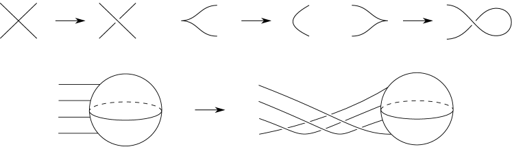
Figure 1. Resolutions of an $xz$-diagram in Gompf standard form.

$1$ at 165 280 $2$ at 165 258 $3$ at 165 235 $4$ at 165 212

$1^{\prime}$ at 165 123 $2^{\prime}$ at 165 92

$1$ at 724 280 $2$ at 724 258 $3$ at 724 235 $4$ at 724 212

$1^{\prime}$ at 724 123 $2^{\prime}$ at 724 92

$1$ at 1200 383 $2$ at 1200 346 $3$ at 1200 307 $4$ at 1200 270

$1^{\prime}$ at 1200 117 $2^{\prime}$ at 1200 80

$4$ at 2015 353 $3$ at 2015 325 $2$ at 2015 295 $1$ at 2015 273

$2^{\prime}$ [b] at 1853 107 $1^{\prime}$ [t] at 1853 84

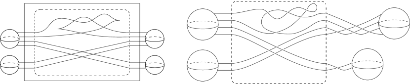
Figure 2. The left gives a Legendrian $xz$-diagram of a link in $\#^{2}(S^{1}\times S^{2})$ in Gompf standard form. The right gives the resolution of the Legendrian link to an $xy$-diagram of a Legendrian isotopic link.

2.2. Definition of the DGA and augmentations in $\#^{k}(S^{1}\times S^{2})$

This section contains an overview of the differential graded algebra over ${\mathbb{Z}}[t^{\pm 1}_{1},\ldots,t^{\pm 1}_{s}]$ presented by Ekholm, Ng in [5]. Let $\Lambda=\Lambda_{1}\coprod\cdots\coprod\Lambda_{n}$ be a Legendrian link in $\#^{k}(S^{1}\times S^{2})$, where the $\Lambda_{i}$ denote the components of $\Lambda$ and $n\leq s$. Let $N_{i}\geq 1$ be the number of strands of $\Lambda$ which go through the $i$-th $1$-handle with $N=\sum N_{i}$ the total number of strands at $x=0$.

2.3. Internal DGA

We will define the internal DGA for a Legendrian link in $S^{1}\times S^{2}$, but one can easily extend the definition to the internal DGA for a Legendrian link in $\#^{k}(S^{1}\times S^{2})$ by defining the internal DGA as follows for each $1$-handle separately.

Let $(r_{1},\ldots,r_{n})\in{\mathbb{Z}}^{n}$ be the $n$-tuple where $r_{i}$ is the rotation number of the $i$-th component $\Lambda_{i}$ and let $(m(1),\ldots,m(N))\in{\mathbb{Z}}^{N}$ be the $N$-tuple of a choice of Maslov potential for each strand passing through the $1$-handle (see §2.5).

Let $(\mathcal{A}_{N},\partial_{N})$ denote the DGA defined as follows. Let $\mathcal{A}$ be the tensor algebra over $R={\mathbb{Z}}[t^{\pm 1}_{1},\ldots,t^{\pm 1}_{s}]$ generated by $c^{0}_{ij}$ for $1\leq i<j\leq N$ and $c^{p}_{ij}$ for $1\leq i,j\leq N$ and $p\geq 1$. Set $\lvert t_{i}\rvert=-2r_{i}$, $\lvert t_{i}^{-1}\rvert=2r_{i}$, and

$$\lvert c^{p}_{ij}\rvert=2p-1+m(i)-m(j)$$

for all $i,j,p$. Define the differential $\partial_{N}$ on the generators by

$$\partial_{N}(c^{0}_{ij}) =\sum_{\ell=i+1}^{j-1}(-1)^{\lvert c^{0}_{i\ell}\rvert+1}c^{0}_{i\ell}c^{0}_{\ell j}$$

$$\partial_{N}(c^{1}_{ij}) =\delta_{ij}+\sum_{\ell=i+1}^{N}(-1)^{|c^{0}_{i\ell}\rvert+1}c^{0}_{i\ell}c^{1}_{\ell j}+\sum_{\ell=1}^{j-1}(-1)^{\lvert c^{1}_{i\ell}\rvert+1}c^{1}_{i\ell}c^{0}_{\ell j}$$

$$\partial_{N}(c^{p}_{ij}) =\sum_{\ell=0}^{p}\sum_{m=1}^{N}(-1)^{\lvert c^{\ell}_{im}\rvert+1}c^{\ell}_{im}c^{p-\ell}_{mj}$$

where $p\geq 2$, $\delta_{ij}$ is the Kronecker delta function, and we set $c^{0}_{ij}=0$ for $i\geq j$. Extend $\partial_{N}$ to $\mathcal{A}_{N}$ by the Leibniz rule

$$\partial_{N}(xy)=(\partial_{N}(x))y+(-1)^{\lvert x\rvert}x(\partial_{N}y).$$

From [5], we know $\partial_{N}$ has degree $-1$, $\partial_{N}^{2}=0$, and $(\mathcal{A}_{N},\partial_{N})$ is infinitely generated as an algebra, but is a filtered DGA, where $c^{p}_{ij}$ is a generator of the $\ell$-th component of the filtration if $p\leq\ell$.

Given a Legendrian link $\Lambda\subset\#^{k}(S^{1}\times S^{2})$, we can associate a DGA $(\mathcal{A}_{N_{i}},\partial_{N_{i}})$ to each of the $1$-handles. We then call the DGA generated by the collection of generators of $\mathcal{A}_{i}$ for $1\leq i\leq k$ with differential induced by $\partial_{N_{i}}$, the internal DGA of $\Lambda$.

2.4. Algebra

Suppose we have a Legendrian link $\Lambda=\Lambda_{1}\coprod\cdots\coprod\Lambda_{n}\subset\#^{k}(S^{1}\times S^{2})$ in normal form with exactly one point labeled $*_{i}$ within the tangle (away from crossings) on each link component $\Lambda_{i}$ of $\Lambda$ (corresponding to $t_{i}$). We will discuss the case where there is more than one base point on a given component in §2.11.

Notation 2.2.

Let $\tilde{a}_{1},\ldots,\tilde{a}_{m}$ denote the crossings of the tangle diagram in normal form. Label the $k$ $1$-handles in the diagram by $1,\ldots,k$ from top to bottom. Recall that $N_{i}$ denotes the number of strands of the tangle going through the $i$-th $1$-handle. For each $i$, label the strands going through the $i$-th $1$-handle on the left side of the diagram $1,\ldots,N_{i}$ from top to bottom and from bottom to top on the right side, as in Figure 2.

Let $\mathcal{A}(\Lambda)$ be the tensor algebra over $R={\mathbb{Z}}[t^{\pm 1}_{1},\ldots,t^{\pm 1}_{s}]$ generated by

• $\tilde{a}_{1},\ldots,\tilde{a}_{m}$;

• $c^{0}_{ij;\ell}$ for $1\leq\ell\leq k$ and $1\leq i<j\leq N_{\ell}$;

• $c^{p}_{ij;\ell}$ for $1\leq\ell\leq k$, $p\geq 1$, and $1\leq i,j\leq N_{\ell}$.

(In general, we will drop the index $\ell$ when the $1$-handle is clear.)

2.5. Grading

The following are a few preliminary definitions which will allow us to define the grading on the generators of $\mathcal{A}(\Lambda)$.

Definition 2.3.

A path in $\pi_{xy}(\Lambda)$ is a path that traverses part (or all) of $\pi_{xy}(\Lambda)$ which is connected except for where it enters a $1$-handle, meaning, where it approaches $x=0$ (respectively $x=A$) along a labeled strand and exits the $1$-handle along the strand with the same label from $x=A$ (respectively $x=0$). Note that the tangent vector in ${\mathbb{R}}^{2}$ to the path varies continuously as we traverse a path as the strands entering and exiting $1$-handles are horizontal.

The rotation number $r(\gamma)$ of a path $\gamma$ is the number of counterclockwise revolutions around $S^{1}$ made by the tangent vector $\gamma^{\prime}(t)/\lvert\gamma^{\prime}(t)\rvert$ to $\gamma$ as we transverse $\gamma$. Generally this will be a real number, but will be an integer if and only if $\gamma$ is smooth and closed.

Thus, the rotation number $r_{i}=r(\Lambda_{i})$ is the rotation number of the path in $\pi_{xy}(\Lambda)$ which begins at the base point $*_{i}$ on the link component $\Lambda_{i}$ and traverses the link component, following the orientation of the component. In the case where $\Lambda$ is a link with components $\Lambda_{1},\ldots,\Lambda_{n}$, we define

$$r(\Lambda)=\gcd(r_{1},\ldots,r_{n}).$$

Define

$$\lvert t_{i}\rvert=-2r(\Lambda_{i}).$$

If $\pi_{xy}(\Lambda)$ is the resolution of an $xz$-diagram of an $n$-component link in Gompf standard form, then the method assigning gradings follows: Choose a Maslov potential $m$ that associates an integer modulo $2r(\Lambda)$ to each strand in the tangle $T$ associated to $\Lambda$, minus cusps and base points, such that the following conditions hold:

1. for all $1\leq\ell\leq k$ and all $1\leq i\leq N_{\ell}$, the strand labeled $i$ going through the $\ell$-th $1$-handle at $x=0$ and the $x=A$ must have the same Maslov potential;

2. if a strand is oriented to the right, meaning it enters the $1$-handle at $x=A$ and exits at $x=0$, then the Maslov potential of the strand must be even. Otherwise the Maslov potential of the strand must be odd;

3. at a cusp, the upper strand (strand with higher $z$-coordinate) has Maslov potential one more than the lower strand.

The Maslov potential is well-defined up to an overall shift by an even integer for knots. (In [5], Ekholm and Ng give another method for defining the gradings using the rotation numbers of specified paths.)

Set $\lvert t_{i}\rvert=-2r(\Lambda_{i})$ and $\lvert c^{p}_{ij;\ell}\rvert=2p-1+m(i)-m(j)$, where $m(i)$ means the Maslov potential of the strand with label $i$ going through the $\ell$-th $1$-handle. It remains to define the grading on crossings in the tangle, crossings resulting from resolving right cusps, and crossings from the half-twists in the resolution. If $a$ is crossing of tangle $T$, then let

$$\lvert a\rvert=m(S_{o})-m(S_{u}),$$

where $S_{o}$ is the strand which crosses over the strand $S_{u}$ at $a$ in the $xy$-projection of $\Lambda$. If $a$ is a right cusp, define $\lvert a\rvert=1$ (assuming there is not a base point in the loop). If $a$ is a crossing in one of the half-twists in the resolution where strand $i$ crosses over strand $j$ ($i<j$), then

$$\lvert a\rvert=m(i)-m(j).$$

2.6. Differential

It suffices to define the differential $\partial$ on generators and extend by the Leibniz rule. Define $\partial({\mathbb{Z}}[t^{\pm 1}_{1},\ldots,t^{\pm 1}_{s}])=0$. Set $\partial=\partial_{N_{\ell}}$ on $\mathcal{A}_{N_{\ell}}$ as in §2.3.

In [5], the DGA on crossings $a_{i}$ is defined by looking for immersed disks in the $xy$-diagrams of Legendrian links, (see the left diagram in Figure 3). However, Ekholm and Ng note that it is equivalent to look for immersed disks in dip versions of the diagram, (see the right diagram in Figure 3). See Figure 4 for the labeling of the crossings in Figure 3.

$1$ [B] at 207 382 $2$ [B] at 207 345 $3$ [B] at 207 307 $4$ [B] at 207 270

$1^{\prime}$ [B] at 207 117 $2^{\prime}$ [B] at 207 81

$4$ [B] at 1016 361 $3$ [B] at 1016 331 $2$ [B] at 1016 299 $1$ [B] at 1016 273

$2^{\prime}$ [B] at 862 109 $1^{\prime}$ [B] at 862 85

$1$ [B] at 1454 382 $2$ [B] at 1454 345 $3$ [B] at 1454 307 $4$ [B] at 1454 270

$1^{\prime}$ [B] at 1454 117 $2^{\prime}$ [B] at 1454 80

$1$ [B] at 2000 382 $2$ [B] at 2000 346 $3$ [B] at 2000 307 $4$ [B] at 2000 271

$1^{\prime}$ [B] at 2000 118 $2^{\prime}$ [B] at 2000 79

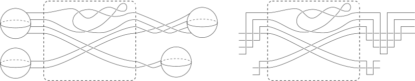
Figure 3. The left gives a Legendrian $xy$-diagram of a link in $\#^{2}(S^{1}\times S^{2})$ which has resulted from the resolution of a link in Gompf standard form. The right gives the dipped version of the link where the half of a dip on the left side of the dipped version is identified with the right half of the dip on the right side. See Figure 4 for the labeling of the crossings in the dips.

$4$ [r] at 0 99 $3$ [r] at 0 132 $2$ [r] at 0 164 $1$ [r] at 0 198

$b_{14}$ [tr] at 100 99 $b_{13}$ [tr] at 100 67 $b_{12}$ [tr] at 100 35 $b_{24}$ [tr] at 68 99 $b_{23}$ [tr] at 68 67 $b_{34}$ [tr] at 37 99

$c^{0}_{14}$ [tl] at 147 99 $c^{0}_{13}$ [tl] at 147 67 $c^{0}_{12}$ [tl] at 147 35 $c^{0}_{24}$ [tl] at 179 99 $c^{0}_{23}$ [tl] at 179 67 $c^{0}_{34}$ [tl] at 212 99

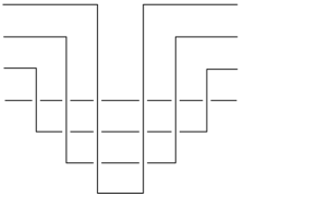
Figure 4. This is the dip at the right of the right figure in Figure 3 with strands and crossings labeled. The labels of the partial dip at the left of the right figure in Figure 3 are the same as the right half of the dip depicted.

Definition 2.4.

Let $a,b_{1},\ldots,b_{\ell}$ be generators. Define $\Delta(a;b_{1},\ldots,b_{\ell})$ to be the set of orientation-preserving immersions

$$f:D^{2}\to{\mathbb{R}}^{2}$$

(up to smooth reparametrization) that map $\partial D^{2}$ to the dip version of $\Lambda$ such that

1. $f$ is a smooth immersion except at $a,b_{1},\ldots,b_{\ell}$,

2. $a,b_{1},\ldots,b_{\ell}$ are encountered as one traverses $f(\partial D^{2})$ counterclockwise,

3. near $a,b_{1},\ldots,b_{\ell}$, $f(D^{2})$ covers exactly one quadrant, specifically, a quadrant with positive Reed sign near $a$ and a quadrant with negative Reeb sign near $b_{1},\ldots,b_{\ell}$, where the Reeb sign of a quadrant near a crossing is defined as in Figure 5.

To each immersed disk, we can assign a word in $\mathcal{A}(\Lambda)$ by starting with the first corner where the quadrant covered has negative Reeb sign, $b_{1}$, and listing the crossing labels of all negative corners as encountered while following the boundary of the immersed polygon counterclockwise, $b_{1}\cdots b_{\ell}$. We associate an orientation sign $\delta_{Q,a}$ to each quadrant $Q$ in the neighborhood of a crossing $a$, defined in Figure 5, and use these to define the sign of a disk $f(D^{2})$ to be the product of the orientation signs over all the corners of the disk. We denote this sign by $\delta(f)$. In many cases there is a unique disk with positive corner at $a$ (with respect to Reeb sign) and negative corners at $b_{1},\ldots,b_{\ell}$ and in these we define $\delta(a;b_{1},\ldots,b_{\ell})$ to be the sign of the unique disk. (In exceptional cases there may be more than one disk with positive corner at $a$ and negative corners at $b_{1},\ldots,b_{\ell}$.)

$-$ [b] at 56 57 $-$ [t] at 56 57 $+$ [l] at 56 57 $+$ [r] at 56 57

$+$ [br] at 248 55 $+$ [tl] at 248 55 $-$ [bl] at 248 55 $-$ [tr] at 248 55

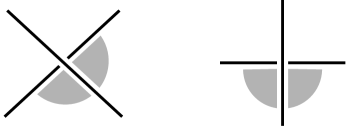
Figure 5. The signs in the figure give the Reeb signs of the quadrants around the crossings. The orientation signs are $+1$ for all quadrants of crossings of odd degree. For crossings of even degree, we use the convention indicated in the left figure if the crossing comes from the $xz$-projection and the convention in the right figure if the crossing is in a dip, which will be discussed in §2.10, where the shaded quadrants have orientation sign $-1$ and the other quadrants have orientation sign $+1$.

Define $n_{*_{i}}(f)$ or $n_{*_{i}}(a;b_{1},\ldots,b_{\ell})$ to be the signed count of the number of times one encounters the base point $*_{i}$ while following $f(\partial D^{2})$ counterclockwise, where the sign is positive if we encounter the base point while following the orientation of the link component and negative if we encounter the base point while going against the orientation.

We define

$$\partial(a_{i})=\sum_{\ell\geq 0}\sum_{(b_{1},\ldots,b_{\ell})}\sum_{f\in\Delta(a_{i};b_{1},\ldots,b_{\ell})}\delta(f)t_{1}^{n_{*_{1}}(f)}\cdots t_{s}^{n_{*_{s}}(f)}b_{1}\cdots b_{\ell}$$

and extend to $\mathcal{A}(\Lambda)$ by the Leibniz rule.

In [5], Ekholm and Ng prove the map $\partial$ has degree $-1$ and is a differential, $\partial^{2}=0$.

$1$ [B] at 174 284 $2$ [B] at 174 260 $3$ [B] at 174 235 $4$ [B] at 174 211

$\bar{1}$ [B] at 174 115 $\bar{2}$ [B] at 174 81

$1$ [B] at 779 284 $2$ [B] at 779 260 $3$ [B] at 779 235 $4$ [B] at 779 211

$\bar{1}$ [B] at 779 115 $\bar{2}$ [B] at 779 81

$1$ [B] at 1189 383 $2$ [B] at 1189 346 $3$ [B] at 1189 307 $4$ [B] at 1189 270

$\bar{1}$ [B] at 1189 117 $\bar{2}$ [B] at 1189 81

$1$ [B] at 1727 383 $2$ [B] at 1727 345 $3$ [B] at 1727 307 $4$ [B] at 1727 270

$\bar{1}$ [B] at 1727 118 $\bar{2}$ [B] at 1727 79

$1$ [b] at 1252 399 $2$ [b] at 1250 302 $3$ [t] at 1249 252

$a_{1}$ [b] at 1400 388 $a_{2}$ [b] at 1509 388 $a_{3}$ [b] at 1441 281 $a_{4}$ [b] at 1570 364 $a_{5}$ [b] at 1600 401 $a_{6}$ [b] at 1408 187 $a_{7}$ [b] at 1448 205 $a_{8}$ [t] at 1439 169 $a_{9}$ [b] at 1481 190

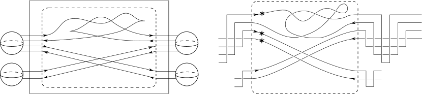
Figure 6. The left gives a Legendrian $xz$-diagram in $\#^{2}(S^{1}\times S^{2})$ in Gompf standard form. The right gives the dip form of the normal form. Recall the labels on the crossings in the dips from Figure 4 for the top $1$-handle and label the left crossing $\bar{b}_{12}$ and the right $\bar{c}_{12}$ in the dip of the bottom $1$-handle.

Example 2.5.

The following is the definition of the DGA $(\mathcal{A}(\Lambda),\partial)$ for the Legendrian link $\Lambda$ in Figure 6. Here $\mathcal{A}(\Lambda)$ is generated by $a_{1},\ldots,a_{9},b_{ij},c^{p}_{ij}$ over ${\mathbb{Z}}[t_{1}^{\pm 1},t_{2}^{\pm 1},t_{3}^{\pm 1}]$. We set $\lvert t_{i}\rvert=2r(\Lambda_{i})=0$ for $i=1,2,3$. Define a Maslov potential $m$ on the strands near $x=0$ by

$$\begin{array}[]{c|*{6}{c}}i&1&2&3&4&\bar{1}&\bar{2}\\ \hline\cr m(i)&2&1&0&-1&0&-1\end{array}$$

Then we have the following gradings: $\lvert a_{1}\rvert=\lvert a_{2}\rvert=\lvert a_{3}\rvert=\lvert a_{7}\rvert=\lvert a_{8}\rvert=0$, $\lvert a_{4}\rvert=\lvert a_{5}\rvert=\lvert a_{9}\rvert=1$, $\lvert a_{6}\rvert=-1$,

$$\begin{array}[]{c|*{7}{C{.15in}}}ij&12$\@add@centering&13$\@add@centering&14$\@add@centering&23$\@add@centering&24$\@add@centering&34$\@add@centering&\widebar{12}$\@add@centering\cr\hline\cr\lvert b_{ij}\rvert&1$\@add@centering&2$\@add@centering&3$\@add@centering&2$\@add@centering&2$\@add@centering&1$\@add@centering&1$\@add@centering\cr\lvert c^{0}_{ij}\rvert&0$\@add@centering&1$\@add@centering&2$\@add@centering&0$\@add@centering&1$\@add@centering&0$\@add@centering&0$\@add@centering\end{array}$$

$$\begin{array}[]{*{6}{C{.15in}}}$\@add@centering&$\@add@centering&\lx@intercol\hfil j\hfil\lx@intercol\\ $\@add@centering&\lx@intercol\hfil\lvert c^{1}_{ij}\rvert\hfil\lx@intercol\vrule\lx@intercol&1$\@add@centering&2$\@add@centering&3$\@add@centering&4$\@add@centering\cr\cline{2-6}\cr\hbox{\multirowsetup i}$\@add@centering&\lx@intercol\hfil 1\hfil\lx@intercol\vrule\lx@intercol&1$\@add@centering&2$\@add@centering&3$\@add@centering&4$\@add@centering\cr$\@add@centering&\lx@intercol\hfil 2\hfil\lx@intercol\vrule\lx@intercol&0$\@add@centering&1$\@add@centering&2$\@add@centering&3$\@add@centering\cr$\@add@centering&\lx@intercol\hfil 3\hfil\lx@intercol\vrule\lx@intercol&-1$\@add@centering&0$\@add@centering&1$\@add@centering&2$\@add@centering\cr$\@add@centering&\lx@intercol\hfil 4\hfil\lx@intercol\vrule\lx@intercol&-2$\@add@centering&-1$\@add@centering&0$\@add@centering&1$\@add@centering\end{array}\hskip 72.26999pt\begin{array}[]{*{6}{C{.15in}}}$\@add@centering&$\@add@centering&\lx@intercol\hfil j\hfil\lx@intercol\\ $\@add@centering&\lx@intercol\hfil\lvert c^{2}_{ij}\rvert\hfil\lx@intercol\vrule\lx@intercol&1$\@add@centering&2$\@add@centering&3$\@add@centering&4$\@add@centering\cr\cline{2-6}\cr\hbox{\multirowsetup i}$\@add@centering&\lx@intercol\hfil 1\hfil\lx@intercol\vrule\lx@intercol&3$\@add@centering&4$\@add@centering&5$\@add@centering&6$\@add@centering\cr$\@add@centering&\lx@intercol\hfil 2\hfil\lx@intercol\vrule\lx@intercol&2$\@add@centering&3$\@add@centering&4$\@add@centering&5$\@add@centering\cr$\@add@centering&\lx@intercol\hfil 3\hfil\lx@intercol\vrule\lx@intercol&1$\@add@centering&2$\@add@centering&3$\@add@centering&4$\@add@centering\cr$\@add@centering&\lx@intercol\hfil 4\hfil\lx@intercol\vrule\lx@intercol&0$\@add@centering&1$\@add@centering&2$\@add@centering&3$\@add@centering\end{array}$$

where $\widebar{12}$ is the crossing of the strands in the bottom $1$-handle. Since $\lvert c^{p}_{ij}\rvert=2p-1+m(i)-m(j)$, we know $\lvert c^{p}_{ij}\rvert>0$ for $p>2$.

For ease of notation, we will use $\bar{c}^{p}_{12}$ to denote $c^{p}_{\widebar{12}}$. We then have the following differentials:

$$\partial a_{1} =\partial a_{2}=\partial a_{3}=\partial a_{6}=0$$

$$\partial a_{4} =(1+a_{2}a_{1})a_{3}-t_{1}^{-1}a_{2}c^{0}_{12}$$

$$\partial a_{5} =1-a_{1}a_{3}+t_{1}^{-1}c^{0}_{12}$$

$$\partial a_{7} =t_{2}^{-1}t_{3}^{-1}c^{0}_{34}a_{6}$$

$$\partial a_{8} =a_{6}\bar{c}^{0}_{12}$$

$$\partial a_{9} =t_{2}^{-1}t_{3}^{-1}c^{0}_{34}a_{8}-a_{7}\bar{c}^{0}_{12}$$

$$\partial b_{12} =1+a_{2}a_{1}-c^{0}_{12}$$

$$\partial b_{13} =(1+a_{2}a_{1})b_{23}+a_{4}(t_{2}c^{0}_{23}a_{7}+t_{3}^{-1}c^{0}_{24}a_{6})-t_{1}^{-1}a_{2}(t_{2}c^{0}_{13}a_{7}+t_{3}^{-1}c^{0}_{14}a_{6})-c^{0}_{13}+b_{12}c^{0}_{23}$$

$$\partial b_{14} =(1+a_{2}a_{1})b_{24}-[a_{4}(t_{2}c^{0}_{23}a_{7}+t_{3}^{-1}c^{0}_{24}a_{6})-t_{1}^{-1}a_{2}(t_{2}c^{0}_{13}a_{7}+t_{3}^{-1}c^{0}_{14}a_{6})]b_{34}$$

$$\quad+(a_{4}c^{0}_{23}-t_{1}^{-1}a_{2}c^{0}_{13})t_{2}a_{9}+(a_{4}c^{0}_{24}-t_{1}^{-1}a_{2}c^{0}_{14})t_{3}^{-1}a_{8}-c^{0}_{14}+b_{12}c^{0}_{24}-b_{13}c^{0}_{34}$$

$$\partial b_{23} =-a_{3}(t_{2}c^{0}_{23}a_{7}+t_{3}^{-1}c^{0}_{24}a_{6})-c^{0}_{23}$$

$$\partial b_{24} =-a_{3}(t_{2}c^{0}_{23}a_{7}+t_{3}^{-1}c^{0}_{24}a_{6})b_{34}-t_{3}^{-1}a_{3}c^{0}_{24}a_{8}-c^{0}_{24}+b_{23}c^{0}_{34}-t_{2}a_{3}c^{0}_{23}a_{9}$$

$$\partial b_{34} =\bar{c}^{0}_{12}-c^{0}_{34}$$

$$\partial\bar{b}_{12} =t_{2}^{-1}t_{3}^{-1}c^{0}_{34}-\bar{c}^{0}_{12}$$

$$\partial c^{p}_{ij} =\delta_{ij}\delta_{1p}+\sum_{\ell=0}^{p}\sum_{m=1}^{4}(-1)^{\lvert c^{\ell}_{im}\rvert+1}c^{\ell}_{im}c^{p-\ell}_{mj}$$

$$\partial\bar{c}^{p}_{ij} =\delta_{ij}\delta_{1p}+\sum_{\ell=0}^{p}\sum_{m=1}^{2}(-1)^{\lvert\bar{c}^{\ell}_{im}\rvert+1}\bar{c}^{\ell}_{im}\bar{c}^{p-\ell}_{mj}$$

Definition 2.6.

Let $(\mathcal{A},\partial)$ be a semifree DGA over $R$ generated by $\{a_{i}|i\in I\}$. Let $J$ be a countable (possibly finite) index set. A stabilization of $(\mathcal{A},\partial)$ is the semifree DGA $(S(\mathcal{A}),\partial)$, where $S(\mathcal{A})$ is the tensor algebra over $R$ generated by $\{a_{i}|i\in I\}\cup\{\alpha_{j}|j\in J\}\cup\{\beta_{j}|j\in J\}$ and the grading on $a_{i}$ is inherited from $\mathcal{A}$ and $\lvert\alpha_{j}\rvert=\lvert\beta_{j}\rvert+1$ for all $j\in J$. Let the differential on $S(\mathcal{A})$ agree with the differential on $\mathcal{A}\subset S(\mathcal{A})$, define

$$\partial(\alpha_{j})=\beta_{j}\text{ and }\partial(\beta_{j})=0$$

for all $j\in J$, and extend by the Leibniz rule.

Definition 2.7.

Two semifree DGAs $(\mathcal{A},\partial)$ and $(\mathcal{A}^{\prime},\partial^{\prime})$ are stable tame isomorphic if some stabilization of $(\mathcal{A},\partial)$ is tamely isomorphic (see [5]) to some stabilization of $(\mathcal{A}^{\prime},\partial^{\prime})$.

Theorem 2.8 ([5] Theorem 2.18).

Let $\Lambda$ and $\Lambda^{\prime}$ be Legendrian isotopic Legendrian links in $\#^{k}(S^{1}\times S^{2})$ in normal form. Let $(\mathcal{A}(\Lambda),\partial)$ and $(\mathcal{A}(\Lambda^{\prime}),\partial^{\prime})$ be the semifree DGAs over $R={\mathbb{Z}}[t^{\pm 1}_{1},\ldots,t^{\pm 1}_{s}]$ associated to the diagrams $\pi_{xy}(\Lambda)$ and $\pi_{xy}(\Lambda^{\prime})$, which are in normal form. Then $(\mathcal{A}(\Lambda),\partial)$ and $(\mathcal{A}(\Lambda^{\prime}),\partial^{\prime})$ are stable tame isomorphic.

Definition 2.9.

Let $F$ be a field. An augmentation of $(\mathcal{A}(\Lambda),\partial)$ to $F$ is a ring map $\epsilon:\mathcal{A}(\Lambda)\to F$ such that $\epsilon\circ\partial=0$ and $\epsilon(1)=1$. If $\rho|2r(\Lambda)$ and $\epsilon$ is supported on generators of degree divisible by $\rho$, then $\epsilon$ is $\rho$-graded. In particular, if $\rho=0$, we say it is graded and if $\rho=1$, we say if is ungraded. We call a generator $a$ augmented if $\epsilon(a)\neq 0$.

Example 2.10.

Recalling the DGA of the Legendrian link in Figure 6 of Example 2.5, given a field $F$, one can check that any graded augmentation $\epsilon$ to $F$ satisfies the following: $\epsilon(t_{1})=-1$, $\epsilon(t_{3})=\epsilon(t_{2})^{-1}$ where $\epsilon(t_{2})\neq 0$, $\epsilon(b_{ij})=\epsilon(\bar{b}_{12})=0$, and for $a,b,c,d,e,f\in F$ such that $1+ab,d,e\neq 0$

$$\begin{array}[]{c|*{9}{C{.1in}}}i&1$\@add@centering&2$\@add@centering&3$\@add@centering&4$\@add@centering&5$\@add@centering&6$\@add@centering&7$\@add@centering&8$\@add@centering&9$\@add@centering\cr\hline\cr\epsilon(a_{i})&a$\@add@centering&b$\@add@centering&-b$\@add@centering&0$\@add@centering&0$\@add@centering&0$\@add@centering&c$\@add@centering&c$\@add@centering&0$\@add@centering\end{array}\hskip 72.26999pt\begin{array}[]{c|*{7}{c}}ij&12&13&14&23&24&34&\widebar{12}\\ \hline\cr\epsilon(c^{0}_{ij})&1+ab&0&0&0&0&d&d\end{array}$$

$$\begin{array}[]{*{6}{c}}&&\lx@intercol\hfil j\hfil\lx@intercol\\ &\lx@intercol\hfil\lvert c^{1}_{ij}\rvert\hfil\lx@intercol\vrule\lx@intercol&1&2&3&4\\ \cline{2-6}\cr\hbox{\multirowsetup i}&\lx@intercol\hfil 1\hfil\lx@intercol\vrule\lx@intercol&0&0&0&0\\ &\lx@intercol\hfil 2\hfil\lx@intercol\vrule\lx@intercol&e&0&0&0\\ &\lx@intercol\hfil 3\hfil\lx@intercol\vrule\lx@intercol&0&f&0&0\\ &\lx@intercol\hfil 4\hfil\lx@intercol\vrule\lx@intercol&0&0&(1+ab)d^{-1}e&0\end{array}\hskip 108.405pt\begin{array}[]{*{6}{c}}&&\lx@intercol\hfil j\hfil\lx@intercol\\ &\lx@intercol\hfil\lvert c^{2}_{ij}\rvert\hfil\lx@intercol\vrule\lx@intercol&1&2&3&4\\ \cline{2-6}\cr\hbox{\multirowsetup i}&\lx@intercol\hfil 1\hfil\lx@intercol\vrule\lx@intercol&0&0&0&0\\ &\lx@intercol\hfil 2\hfil\lx@intercol\vrule\lx@intercol&0&0&0&0\\ &\lx@intercol\hfil 3\hfil\lx@intercol\vrule\lx@intercol&0&0&0&0\\ &\lx@intercol\hfil 4\hfil\lx@intercol\vrule\lx@intercol&-(1+ab)d^{-1}f&0&0&0\end{array}$$

Note that any augmentation of a stabilization $S(\mathcal{A})$ restricts to an augmentation of the smaller algebra $\mathcal{A}$ and any augmentation of the algebra $\mathcal{A}$ extends to an augmentation of the stabilization $S(\mathcal{A})$ where the augmentation sends $\beta_{j}$ to $0$ and $\alpha_{j}$ to an arbitrary element of $F$ if $\rho|\lvert\alpha_{j}\rvert$ and $0$ otherwise for all $j\in J$.

2.7. Normal rulings in $\#^{k}(S^{1}\times S^{2})$

In this section, we extend the definition of a normal ruling from Legendrian links in ${\mathbb{R}}^{3}$ to Legendrian links in $\#^{k}(S^{1}\times S^{2})$. We formulate the definition similarly to how Lavrov and Rutherford [13] define normal rulings in the case of Legendrian links in the solid torus.

Consider the tangle portion of the $\pi_{xz}(\Lambda)$ diagram in normal form of a Legendrian link $\Lambda\subset\#^{k}(S^{1}\times S^{2})$. A normal ruling can be viewed locally as a decomposition of $\pi_{xz}(\Lambda)$ into pairs of paths.

Let $C\subset S^{1}$ be the set of $x$-coordinates of crossings and cusps of $\pi_{xz}(\Lambda)$ where $S^{1}=[0,A]/\{0=A\}$. We can write

$$S^{1}\backslash C=\coprod_{\ell=1}^{M}I_{\ell}$$

where $I_{\ell}$ is an open interval (or all of $S^{1}$) for each $\ell$. We will use the convention that $I_{0}=I_{M}$ and the $I_{\ell}$ are ordered $I_{0},\ldots,I_{M}$ from $x=0$ to $x=A$ (from left to right in the $xz$-diagram) so that $I_{\ell-1}$ appears to the left of (has lower $x$-coordinates than) $I_{\ell}$. Note that $(I_{\ell}\times[-M,M])\cap\pi_{xz}(\Lambda)$ consists of some number of nonintersecting components which project homeomorphically onto $I_{\ell}$. We call these components strands of $\pi_{xz}(\Lambda)$ and number them from top to bottom by $1,\ldots,N(\ell)$. For each $\ell$, choose a point $x_{\ell}\in I_{\ell}$.

Definition 2.11.

A normal ruling of $\pi_{xz}(\Lambda)$ is a sequence of involutions $\sigma=(\sigma_{1},\ldots,\sigma_{M})$,

$$\sigma_{m}:\{1,\ldots,N(m)\}\to\{1,\ldots,N(m)\}$$

$$(\sigma_{m})^{2}=id,$$

satisfying:

1. Each $\sigma_{m}$ is fixed-point-free.

2. If the strands above $I_{m}$ labeled $\ell$ and $\ell+1$ meet at a left cusp in the interval $(x_{m-1},x_{m})$, then

   $$\sigma_{m}(i)=\begin{cases}\ell+1&\text{if }i=\ell,\\ \sigma_{m-1}(i)&\text{if }i<\ell,\\ \sigma_{m-1}(i-2)&\text{if }i>\ell+1.\end{cases}$$

   And a similar condition at right cusps.

3. If strands above $I_{m}$ labeled $\ell$ and $\ell+1$ meet at a crossing on the interval $(x_{m-1},x_{m})$, then $\sigma_{m-1}(\ell)\neq\ell+1$ and either

   • $\sigma_{m}=(\ell\quad\ell+1)\circ\sigma_{m-1}\circ(\ell\quad\ell+1)$ where $(\ell\quad\ell+1)$ denotes transposition or

   • $\sigma_{m}=\sigma_{m-1}$.

   When the second case occurs, we call the crossing switched. We say the normal ruling is $\rho$-graded if $\rho\big{|}\lvert c\rvert$ for all switched crossings $c$.

4. (Normality condition) If there is a switched crossing on the interval $(x_{m-1},x_{m})$, then one of the following holds:

   • $\sigma_{m}(\ell+1)<\sigma_{m}(\ell)<\ell<\ell+1$

   • $\sigma_{m}(\ell)<\ell<\ell+1<\sigma_{m}(\ell)$

   • $\ell<\ell+1<\sigma_{m}(\ell+1)<\sigma_{m}(\ell)$

5. Near $x=0$ and $x=A$, both the strand with label $\ell$ and $\sigma_{0}(\ell)$ must go through the same $1$-handle, in other words, there exists $p$ such that $\sum_{i=1}^{p-1}N_{i}<\ell,\sigma_{0}(\ell)\leq\sum_{i=1}^{p}N_{i}$.

The final condition is the only condition which is different from how normal rulings are defined in [13] for the case of solid torus knots. This condition ensures the ruling “behaves well” with the $1$-handles.

Remark 2.12.

As in [13], one can equivalently see normal rulings as pairings of strands in the $xz$-diagram with certain conditions. Here we think of strands $i$ and $j$ being paired for $x_{m-1}\leq x\leq x_{m}$ if $\sigma_{m}(i)=j$. In this way, we can cover the $xz$-diagram with pairs of paths which have monotonically increasing $x$-coordinate. Note that if a path goes all the way from $x=0$ to $x=A$, it may end up on a different strand than it started, but strand $i$ is paired with strand $j$ at $x=0$ if and only if they are paired at $x=A$. Condition 5 also specifies that the paired strands must go through the same $1$-handle. The conditions mentioned above are as follows: Paired paths can only meet at a cusp. This also means that at a crossing, the crossings strands must be paired with other strands. These companion strands can either lie above or below the crossing. Conditions 3 and 4 specify that near a crossing the pairings must be one of those depicted in Figure 7.

Example 2.13.

Figure 8 gives the normal rulings of the Legendrian link from Example 2.5.

2pt $(a)$ [t] at 82 267 $(b)$ [t] at 339 267 $(c)$ [t] at 593 267 $(d)$ [t] at 82 -20 $(e)$ [t] at 339 -20 $(f)$ [t] at 593 -20

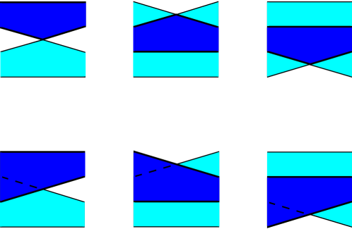
Figure 7. These, along with vertical reflections of (d), (e), and (f), are all possible configurations of a normal ruling near a crossing. The top row contains all possible configurations for switched crossings in a normal ruling. (This figure is taken from [14].)

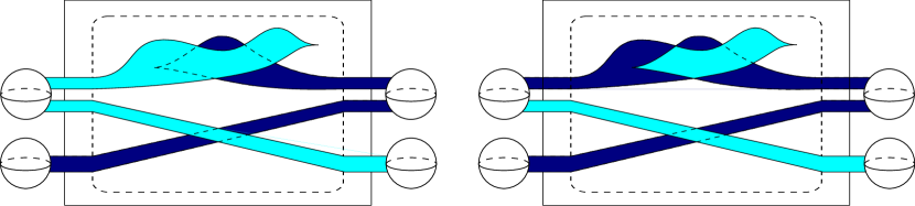
Figure 8. These are the two normal rulings of the Legendrian link of Example 2.5 seen in Figure 6.

Similarly to ${\mathbb{R}}^{3}$, we can define a $\rho$-graded ruling polynomial.

Definition 2.14.

If $m$ is a ${\mathbb{Z}}/\rho$-valued Maslov potential for a Legendrian link $\Lambda$, then the $\rho$-graded ruling polynomial of $\Lambda$ with respect to $m$ is

$$R^{\rho}_{(\Lambda,m)}=\sum_{\sigma}z^{j(\sigma)},$$

where the sum is over all $\rho$-graded normal rulings of $\Lambda$ and

$$j(\sigma)=\text{\# switches}-\text{\# right cusps}.$$

Note that in the case where $\Lambda$ is a knot, the ruling polynomial does not depend on the Maslov potential. Restated from the introduction:

Theorem 1.2.

The $\rho$-graded ruling polynomial $R^{\rho}_{(\Lambda,m)}$ with respect to the Maslov potential $m$ (which changes under Legendrian isotopy) is a Legendrian isotopy invariant.

Proof.

By Gompf [12], any Legendrian link in $\#^{k}(S^{1}\times S^{2})$ can be represented by an $xz$-diagram in Gompf standard form and two such $xz$-diagrams represent links that are Legendrian isotopic if and only if they are related by a sequence of Legendrian Reidemeister moves of the $xz$-diagram of the tangle inside $[0,A]\times[-M,M]$ and three additional moves, which we will, following the nomenclature of [5], call Gompf moves 4, 5, and 6 (see Figure 9). By [3], we know the ruling polynomial is invariant under Legendrian isotopy of the tangle, so we need only show it is invariant under Gompf moves 4, 5, and 6.

2pt $4:$ [r] at -10 1216 ${\large\Lambda}$ at 844 1216

${\large\Lambda}$ at 2873 1216

$5:$ [r] at -10 701 ${\large\Lambda}$ at 844 701

${\large\Lambda}$ at 2873 701

$6:$ [r] at -10 182

${\large\Lambda}$ at 2873 182

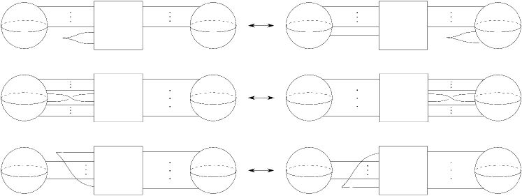
Figure 9. Gompf moves 4, 5, and 6.

Gompf moves 4 and 5 clearly do not change the ruling polynomial. For Gompf move 6, note that any normal ruling cannot pair a strand going through the $1$-handle with one of the strands incident to the cusp. Instead, the ruling must pair the two strands incident to the left cusp and not have any switches in the portion of the diagram depicted in Figure 9, thus the ruling polynomial does not change. ∎

Example 2.15.

The normal rulings for the Legendrian link from Example 2.5 are given in Figure 8. Thus the ruling polynomial is

$$R_{\Lambda}=z^{-1}+z.$$

2.8. Legendrian links in ${\mathbb{R}}^{3}$

The classical invariants for Legendrian isotopy classes of knots in ${\mathbb{R}}^{3}$ are: topological knot type, Thurston-Bennequin number, and rotation number (see [8]). The Thurston-Bennequin number of a knot measures the self-linking of a Legendrian knot $\Lambda$. Given a push off $\Lambda^{\prime}$ of $\Lambda$ in a direction tangent to the contact structure, then $tb(\Lambda)$ is the linking number of $\Lambda$ and $\Lambda^{\prime}$. Given the $xz$-projection of $\Lambda$,

$$tb(\Lambda)=\text{writhe}(\Lambda)-\frac{1}{2}(\text{number of cusps}).$$

The rotation number $r(\Lambda)$ of an oriented Legendrian knot $\Lambda$ is the rotation of its tangent vector field with respect to any global trivialization. (This definition agrees with the definition of the rotation number of a path given earlier.) Given the $xz$-projection of $\Lambda$,

$$r(\Lambda)=\frac{1}{2}(\text{number of down cusps}-\text{number of up cusps}).$$

Given a Legendrian link $\Lambda=\Lambda_{1}\coprod\cdots\coprod\Lambda_{n}$, we define $tb_{i}=tb(\Lambda_{i})$ and $r_{i}=r(\Lambda_{i})$ for $1\leq i\leq n$ and define

$$r(\Lambda)=\gcd(r_{1},\ldots,r_{n}).$$

2.9. Satellites, the DGA, and augmentations in ${\mathbb{R}}^{3}$

This section gives the results and notation for Legendrian links in ${\mathbb{R}}^{3}$ necessary to prove Theorem 1.3.

We will first extend the idea of satelliting a knot in $J^{1}(S^{1})$ to an unknot (see [16]) to satelliting each $1$-handle of a knot in $\#^{k}(S^{1}\times S^{2})$ around a twice stabilized unknot.

Definition 2.16.

Given the $xy$- or $xz$-diagram for a Legendrian link $\Lambda$ in $\#^{k}(S^{1}\times S^{2})$, satellited $\Lambda$ is denoted $S(\Lambda)$, the $xy$-diagram of which is depicted in Figure 10 and the $xz$-diagram of a Legendrian isotopic link of which is depicted in Figure 12 for the Legendrian link from Figure 6. Label the crossings as indicated, where $i\leq j$ and label the base points in $S(\Lambda)$ as they are labeled in $\Lambda$. Note that the $xy$- or $xz$-diagram of $\Lambda$ defines $S(\Lambda)$ up to Legendrian isotopy.

$1$ [b] at 750 1954 $2$ [b] at 750 1889 $3$ [b] at 750 1824 $4$ [b] at 750 1758

$\bar{1}$ [b] at 750 1488 $\bar{2}$ [b] at 750 1423

$1$ [b] at 1708 1963 $2$ [b] at 1708 1898 $3$ [b] at 1708 1829 $4$ [b] at 1708 1767

$\bar{1}$ [b] at 1708 1498 $\bar{2}$ [b] at 1708 1432

$t_{1}$ [b] at 879 1993 $t_{2}$ [B] at 879 1840 $t_{3}$ [t] at 878 1755

$a_{1}$ [b] at 1129 1975 $a_{2}$ [b] at 1321 1975 $a_{3}$ [b] at 1201 1784 $a_{4}$ [b] at 1430 1929 $a_{5}$ [b] at 1490 1998 $a_{6}$ [b] at 1144 1618 $a_{7}$ [b] at 1212 1653 $a_{8}$ [b] at 1200 1589 $a_{9}$ [b] at 1273 1625

$b_{ij}$ at 1764 1660 $c_{ij}$ at 2043 1665 $\bar{b}_{12}$ [tr] at 1741 1431 $\bar{c}_{12}$ [tl] at 1804 1432

$d_{ji}$ [l] at 2748 1571 $e_{ij}$ [r] at 2254 1100 $f_{ji}$ [l] at 2720 712 $g_{ij}$ [r] at 7 699 $h_{ji}$ [l] at 450 1131 $q_{ij}$ [r] at 8 1592

$\bar{d}_{ji}$ [l] at 2120 1307 $\bar{e}_{12}$ [r] at 1825 1116 $\bar{f}_{ji}$ [l] at 2118 934 $\bar{g}_{12}$ [r] at 640 937 $\bar{h}_{ji}$ [l] at 899 1108 $\bar{q}_{12}$ [r] at 622 1329

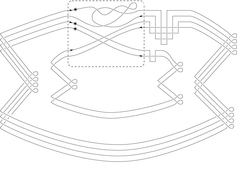
Figure 10. The $xy$-projection of the satellited link $S(\Lambda)$. The crossings in the $c_{ij}$-, $b_{ij}$-, $\bar{c}_{ij}$, and $\bar{b}_{ij}$-lattices are labeled as in Figure 4. The crossings in the $d,e,f,g,h,q$-lattices are labelled according to Figure 11.

$1$ [b] at 196 381 $2$ [b] at 255 381 $3$ [b] at 312 381 $4$ [b] at 372 381

$1$ [t] at 395 7 $2$ [t] at 329 7 $3$ [t] at 262 7 $4$ [t] at 195 7

$e_{12}$ [b] at 142 268 $e_{13}$ [b] at 175 237 $e_{14}$ [b] at 208 205 $e_{23}$ [b] at 143 201 $e_{24}$ [b] at 175 170 $e_{34}$ [b] at 144 136

$1$ [b] at 892 381 $2$ [b] at 840 381 $3$ [b] at 788 381 $4$ [b] at 738 381

$1$ [t] at 724 7 $2$ [t] at 780 7 $3$ [t] at 837 7 $4$ [t] at 893 7

$d_{11}$ [b] at 971 303 $d_{21}$ [b] at 937 268 $d_{31}$ [b] at 910 238 $d_{41}$ [b] at 883 207 $d_{22}$ [b] at 970 237 $d_{32}$ [b] at 937 203 $d_{42}$ [b] at 910 170 $d_{33}$ [b] at 971 171 $d_{43}$ [b] at 937 137 $d_{44}$ [b] at 968 107

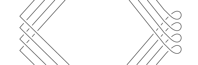
Figure 11. The labels for the crossings in the $e$- and $d$-lattices of the satellited link $S(\Lambda)$ as seen in Figure 10. The $f$- and $h$-lattices are analogous to the $d$-lattice. The $g$- and $q$-lattices are analogous to the $e$-lattice.

$1$ [B] at 543 824 $2$ [B] at 543 801 $3$ [B] at 543 779 $4$ [B] at 543 757

$1^{\prime}$ [B] at 543 658 $2^{\prime}$ [B] at 543 628

$1$ [B] at 1210 825 $2$ [B] at 1210 802 $3$ [B] at 1210 780 $4$ [B] at 1210 757

$1^{\prime}$ [B] at 1210 664 $2^{\prime}$ [B] at 1210 633

$a_{1}$ [b] at 833 888 $a_{2}$ [b] at 927 891 $a_{3}$ [b] at 865 825 $a_{4}$ [b] at 989 855 $a_{5}$ [l] at 1074 891 $a_{6}$ [b] at 809 710 $a_{7}$ [b] at 874 724 $a_{8}$ [b] at 874 696 $a_{9}$ [b] at 939 710

$d_{ji}$ [l] at 1737 653 $e_{ij}$ [r] at 1342 433 $f_{ji}$ [l] at 1736 232 $g_{ij}$ [r] at 8 232 $h_{ji}$ [l] at 393 434 $q_{ij}$ [r] at 8 652

$d^{\prime}_{ji}$ [l] at 1342 541 $e^{\prime}_{ij}$ [r] at 1153 431 $f^{\prime}_{ji}$ [l] at 1342 318 $g^{\prime}_{ij}$ [r] at 402 321 $h^{\prime}_{ji}$ [l] at 588 430 $q^{\prime}_{ij}$ [r] at 402 542

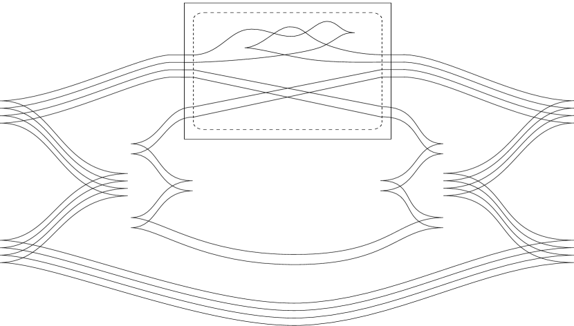
Figure 12. The $xz$-projection of a link which is Legendrian isotopic to the satellited link $S(\Lambda)$.

Remark 2.17.

The Chekanov-Eliashberg DGA was originally defined on Legendrian links in $({\mathbb{R}}^{3},dz-ydx)$ (see [4],[18]). Note that the same DGA results from defining the DGA as we did in $\#^{k}(S^{1}\times S^{2})$ where $k=0$.

2.10. Dips

Dips will be defined analogously to those defined in [14].

Given a diagram $\pi_{xy}(\Lambda)$ in normal form which is the result of resolution, we construct a dip in the vertical slice of the diagram between two crossings, a crossing and a cusp, or two cusps, by a sequence of Reidemeister II moves, as seen in Figure 13 in the $xz$-projection and $xy$-projection. From the $xz$-projection, it is clear that the diagram with the dip is Legendrian isotopic to the original diagram. To construct a dip, number the $N$ strands from top to bottom. Using a type II Reidemeister move, push strand $N-1$ over strand $N$, then strand $N-2$ over strand $N-1$, then strand $N-2$ over strand $N$, and so on. In this way, strand $i$ is pushed over strand $j$ in anti-lexicographic order.

1pt $4$ [r] at 320 99 $3$ [r] at 320 132 $2$ [r] at 320 164 $1$ [r] at 320 198

$b_{14}$ [tr] at 425 99 $b_{13}$ [tr] at 425 67 $b_{12}$ [tr] at 425 35 $b_{24}$ [tr] at 393 99 $b_{23}$ [tr] at 393 67 $b_{34}$ [tr] at 362 99

$c_{14}$ [tl] at 472 99 $c_{13}$ [tl] at 472 67 $c_{12}$ [tl] at 472 35 $c_{24}$ [tl] at 505 99 $c_{23}$ [tl] at 505 67 $c_{34}$ [tl] at 537 99

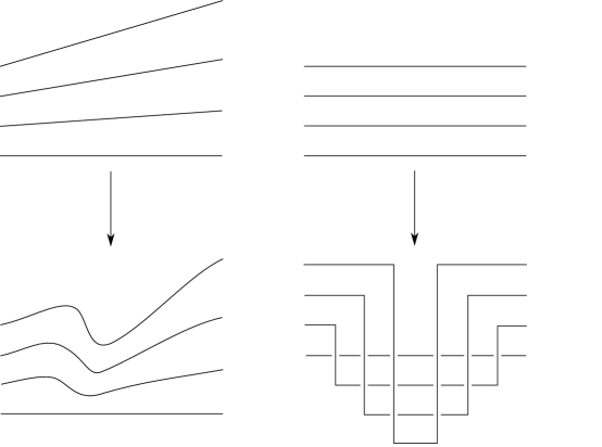
Figure 13. The left diagram gives the modification of the $xz$-diagram when creating a dip. The right diagram gives the modification of the $xy$-diagram. (This figure is taken from [14].)

Given an $xy$-diagram for a link $\Lambda\subset{\mathbb{R}}^{3}$ in normal form, where all crossings and resolutions of left cusps having distinct $x$-coordinates, the dipped diagram $D(\Lambda)$ is the result of adding a dip between each pair of crossings or resolution of a cusp and crossing. For each Reidemeister II move, we have two new generators. Call the left crossing $b_{ij}$ and the right crossing $c_{ij}$ if strands $i<j$ cross. One can check that $\lvert b_{ij}\rvert=m(j)-m(i)$ and since $\partial$ lowers degree by $1$, we know $\lvert c_{ij}\rvert=\lvert b_{ij}\rvert-1$.

While dipped diagrams have many more crossings than the original link diagram, the differential $\partial$ on $\mathcal{A}(D(\Lambda))$ is generally much simpler. In fact, a totally augmented disk (a disk from the definition of the differential of the DGA where all crossings at corners are augmented), cannot “go through” or “span” more than one dip.

2.11. Augmentations before and after base points and type II moves

In some cases, we will find that adding base points will simplify the signs. For Legendrian links in ${\mathbb{R}}^{3}$, Ng and Rutherford give the DGA isomorphisms induced by adding a base point to a diagram and by moving a base point around a link in [16]. One can easily extend their results to $\#^{k}(S^{1}\times S^{2})$. In the case where a base point is pushed through a crossing $c_{i}$, the DGA isomorphism sends $c_{i}$ to $t_{j}^{\pm 1}c_{i}$, the sign depending on whether the base point is pushed along the link with or against the orientation of the strand, and preserves $c_{j}$ if no base point is pushed through $c_{j}$. If a base point $*_{i}$ corresponding to $t_{i}$ is added next to a base point $*$ corresponding to $t$, then the DGA homomorphism sends $t$ to $tt_{i}^{-1}$. Given an augmentation of the DGA of the diagram before either operation, this DGA isomorphism clearly gives us an augmentation of the DGA of the new diagram.

Remark 2.18.

In summary, if we have an augmentation $\epsilon:\mathcal{A}\to F$ with $\epsilon(t_{i})=-1$, then moving the base point $*_{i}$ through a crossing $c_{j}$ only changes the augmentation by changing the sign of the augmentation on the crossing $c_{j}$. Suppose we have a diagram with a base point $*$ corresponding to $t$ and the same diagram with base points $*_{1},\ldots,*_{s}$ associated to $t_{1},\ldots,t_{s}$ on the same component of the link and we move all of the base points $*_{1},\ldots,*_{s}$ to the location of $*$. By the above results, if $\epsilon$ is an augmentation to $F$ of the multiple base point diagram, there exists an augmentation $\epsilon^{\prime}$ to $F$ of the single base point diagram such that for all crossings $c$ there exists $x_{c}\in F$ such that $\epsilon^{\prime}(c)=x_{c}\epsilon(c)$ and

$$\epsilon^{\prime}(t)=\epsilon(t_{1}\ldots t_{s})=\prod_{i=1}^{s}\epsilon(t_{i}).$$

In [9], Etnyre, Ng, and Sabloff give a DGA isomorphism relating the DGA of a diagram of a Legendrian knot in ${\mathbb{R}}^{3}$ before and after a Reidemeister II move. One can easily extend this to a similar result for $\#^{k}(S^{1}\times S^{2})$, which gives a way to extend an augmentation of the diagram before a Reidemeister II move to an augmentation of the diagram after the move, (see [14] for the analogous result in ${\mathbb{R}}^{3}$).

3. Correspondence between augmentations and normal rulings for links in ${\mathbb{R}}^{3}$

From [14], we have the following result for knots in ${\mathbb{R}}^{3}$.

Theorem 3.1 ([14] Theorem 1.1).

Let $\Lambda$ be a Legendrian knot in ${\mathbb{R}}^{3}$. Given a field $F$, $(\mathcal{A},\partial)$ has a $\rho$-graded augmentation $\epsilon:\mathcal{A}\to F$ if and only if any front diagram of $\Lambda$ has a $\rho$-graded normal ruling. Furthermore, if $\rho$ is even, then $\epsilon(t)=-1$.

This result is proven by construction. Using the same method we can prove an analogous result for links in ${\mathbb{R}}^{3}$. Restating from the introduction:

Theorem 1.1.

Let $\Lambda$ be an $n$-component Legendrian link in ${\mathbb{R}}^{3}$ with $s$ base points (at least one base point on each component). Given a field $F$, the Chekanov-Eliashberg DGA $(\mathcal{A},\partial)$ over ${\mathbb{Z}}[t_{1}^{\pm 1},\ldots,t_{s}^{\pm 1}]$ has a $\rho$-graded augmentation $\epsilon:\mathcal{A}\to F$ if and only if a front diagram of $\Lambda$ has a $\rho$-graded normal ruling. Furthermore, if $\rho$ is even, then $\epsilon(t_{1}\cdots t_{s})=(-1)^{s}$.

The following result will be necessary for the proof of Theorem 1.1. Analogous to the knot case in ${\mathbb{R}}^{3}$, we have the following extension of Lemma 3.2 from ([14]):

Lemma 3.2.

If $c$ gives the number of right cusps, $sw$ is the number of switches in the ruling, $a_{-}$ is the number of $-$(a) crossings, and $n$ the number of components then

$$c+sw+a_{-}\equiv n\mod 2.$$

Proof.

As in the knot case, one can easily show each of the following statements:

(1) $$\sum_{i=1}^{n}tb_{i}+\sum_{i=1}^{n}r_{i}\equiv n\mod 2$$

(2) $$\sum_{i=1}^{n}tb_{i}\equiv c+cr\mod 2$$

(3) $$cr\equiv sw\mod 2$$

(4) $$\sum_{i=1}^{n}r_{i}\equiv a_{-}\mod 2$$

where $r_{i}$ is the rotation number of $\Lambda_{i}$ and $cr$ is the number of crossings. Note that if we add these four equations together, we get that

$$c+sw+a_{-}\equiv n\mod 2$$

as desired. ∎

Proof of Theorem 1.1.

After a series of Legendrian isotopies, we can assume the front diagram of $\Lambda$ has the following form where from left to right (lowest $x$-coordinate to highest $x$-coordinate) we have: all left cusps have the same $x$-coordinate, no two crossings of $\Lambda$ have the same $x$-coordinate, and all right cusps have the same $x$-coordinate (in [14], this is called plat position). Label the crossings in the right cusps by $q_{1},\ldots,q_{m}$ from top to bottom and label the other crossings by $c_{1},\ldots,c_{\ell}$ from left to right.

(Augmentation to ruling) Given a $\rho$-graded augmentation of the Chekanov-Eliashberg DGA of the resolution of $\pi_{xz}(\Lambda)$ to a Lagrangian diagram. Define a $\rho$-graded normal ruling of $\pi_{xz}(\Lambda)$ by simultaneously defining a $\rho$-graded augmentation of the dipped diagram $D(\Lambda)$ as in the knot case, using Figure 14.

(Ruling to augmentation) Given a $\rho$-graded normal ruling of $\pi_{xz}(\Lambda)$. Define a $\rho$-graded augmentation of the dipped diagram $D(\Lambda)$ with base points where specified in Figure 14 and at each right cusps as in the knot case, using Figure 14.

Using Lemma 3.2 and the methods in the proof of Theorem 3.1 in [14], one can show the final statement of Theorem 1.1. Given a $\rho$-graded augmentation $\epsilon:\mathcal{A}\to F$, consider the associated $\rho$-graded normal ruling. If $\rho$ is even, then the ruling is only switched at crossings $c_{k}$ with $\rho\big{|}\lvert c_{k}\rvert$ and so $2\big{|}\lvert c_{k}\rvert$. Thus, any strands paired by the ruling must have opposite orientation. As in the case of knots, this implies that near a crossing where the ruling is switched the crossing must be a positive crossing. Thus each ruling path is an oriented unknot.

If we consider the dipped diagram of the link, by induction we can show that

$$\prod\left(\epsilon(b^{k}_{ij})^{\pm 1}\right)=1,$$

where the product is taken over all paired strands $i$ and $j$ in the ruling between $c_{k}$ and $c_{k+1}$ and the sign is determined by the orientation of the paired strands as in [14]. By considering $\partial q_{k}$, we see that

$$\epsilon(t_{1}\cdots t_{s}) =(-1)^{s-m}\prod_{k=1}^{m}\left(-(\epsilon(b^{\ell}_{2k,2k-1}))^{\pm 1}\right)$$

$$=(-1)^{s}\prod_{i<j\text{ paired}}\left(\epsilon(b^{\ell}_{ij})^{\pm 1}\right)$$

$$=(-1)^{s}$$

$$=(-1)^{n}$$

by Lemma 3.2 and the fact that the number of base points $s\equiv c+sw+a_{-}\mod 2$. ∎

4. Augmentation to Ruling

In this section, we will show that the DGA of a Legendrian link $\Lambda$ in $\#^{k}(S^{1}\times S^{2})$ is a subalgebra of the DGA of satellited $\Lambda$ in ${\mathbb{R}}^{3}$ and use the construction from Theorem 1.1 [14] to construct a ruling of the satellited link in ${\mathbb{R}}^{3}$ to then give a normal ruling of $\Lambda$ in $\#^{k}(S^{1}\times S^{2})$. This shows the forward direction of Theorem 1.3.

Given an $xy$-diagram for the Legendrian link $\Lambda$ in $\#^{k}(S^{1}\times S^{2})$ which results from the resolution of an $xz$-diagram in normal form with base points indicated. We can construct an $xy$-diagram for $S(\Lambda)$, satellited $\Lambda$, (see Figure 10) with base points in the same location as they were for $\Lambda$.

We will use the notation for Legendrian links in $\#^{k}(S^{1}\times S^{2})$ with tildes added for the Legendrian link $\Lambda$ in $\#^{k}(S^{1}\times S^{2})$: $\mathcal{A}(\Lambda)={\mathbb{Z}}[\tilde{t}_{1}^{\pm 1},\ldots,\tilde{t}_{s}^{\pm 1}]\langle\tilde{a}_{i},\tilde{b}_{ij;\ell},\tilde{c}^{p}_{ij;\ell}\rangle$ with differential $\tilde{\partial}$, where $1\leq\ell\leq k$, $i<j$ for all $\tilde{b}_{ij;\ell}$, $i<j$ for $\tilde{c}^{p}_{ij;\ell}$ if $p=1$, and $i\leq j$ if $p>1$. We will use the notation for Legendrian links from Figure 10 for $S(\Lambda)$:

$$\mathcal{A}(S(\Lambda))={\mathbb{Z}}[t_{1}^{\pm 1},\ldots,t_{s}^{\pm 1}]\langle a_{i},b_{ij;\ell},c_{ij;\ell},d_{ji;\ell},e_{ij;\ell},f_{ji;\ell},g_{ij;\ell},h_{ji;\ell},q_{ij;\ell}\rangle$$

with differential $\partial$, where $1\leq\ell\leq k$, $1\leq i\leq m$ for $a_{i}$, $i<j$ for $b_{ij;\ell}$, $c_{ij;\ell}$, $e_{ij;\ell}$, $g_{ij;\ell}$, and $q_{ij;\ell}$, and $i\leq j$ for $d_{ji;\ell}$, $f_{ji;\ell}$, and $h_{ji;\ell}$.

Note that

$$\partial a_{i} =\tilde{\partial}\tilde{a}_{i}\rvert_{\tilde{a}_{r}=a_{r},\tilde{c}^{0}_{rs;p}=q_{rs;p},\tilde{t}_{r}=t_{r}},$$

$$\partial b_{ij;\ell} =\tilde{\partial}\tilde{b}_{ij;\ell}\rvert_{\tilde{a}_{r}=a_{r},\tilde{b}_{rs;p}=b_{rs;p},\tilde{c}^{0}_{rs;p}=q_{rs;p},\tilde{t}_{r}=t_{r}},$$

and in the $p$-th $1$-handle

$$\partial c_{ij} =\tilde{\partial}\tilde{c}^{0}_{ij}\rvert_{\tilde{c}^{0}_{rs}=c_{rs}},$$

where $1\leq i<j\leq N_{p}$. One can check that in the $p$-th $1$-handle

$$\partial e_{ij}=\sum_{i<\ell<j}(-1)^{\lvert e_{i\ell}\rvert+1}e_{i\ell}e_{\ell j}=\tilde{\partial}\tilde{c}^{0}_{ij}\rvert_{\tilde{c}^{0}_{rs}=e_{rs}}$$

for $1\leq i<j\leq N_{p}$. Similarly

$$\partial g_{ij} =\tilde{\partial}\tilde{c}^{0}_{ij}\rvert_{\tilde{c}^{0}_{rs}=g_{rs}},$$

$$\partial q_{ij} =\tilde{\partial}\tilde{c}^{0}_{ij}\rvert_{\tilde{c}^{0}_{rs}=q_{rs}}.$$

One can also check that

$$\partial d_{ji} =\delta_{ij}+\sum_{j<\ell\leq N_{p}}c_{j\ell}d_{\ell i}+\sum_{1\leq\ell<i}(-1)^{\lvert d_{j\ell}\rvert+1}d_{j\ell}e_{\ell i},$$

$$\partial f_{ji} =\delta_{ij}+\sum_{j<\ell\leq N_{p}}(-1)^{\lvert e_{j\ell}\rvert+1}e_{j\ell}f_{\ell i}+\sum_{1\leq\ell<i}(-1)^{\lvert f_{j\ell}\rvert+\lvert g_{\ell i}\rvert}f_{j\ell}g_{\ell i},$$

$$\partial h_{ji} =\delta_{ij}+\sum_{j<\ell\leq N_{p}}(-1)^{\lvert q_{j\ell}\rvert+1}q_{j\ell}h_{\ell i}+\sum_{1\leq\ell<i}(-1)^{\lvert h_{j\ell}\rvert+1}h_{j\ell}g_{\ell i},$$

where $1\leq i\leq j\leq N_{p}$.

Remark 4.1.

Suppose we have a Legendrian link $\Lambda$ in $\#^{k}(S^{1}\times S^{2})$ with associated DGA $(\mathcal{A}(\Lambda),\partial)$. If $(\mathcal{A}(S(\Lambda)),\partial)$ is the DGA associated to satellited $\Lambda$, then we have

where the final map is inclusion and

$$B=R\langle c_{ij;\ell}-g_{ij;\ell},c_{ij;\ell}-q_{ij;\ell},c_{ij;\ell}-(-1)^{\lvert e_{ij;\ell}\rvert+1}e_{ij;\ell},h_{ji;\ell}-(-1)^{\lvert f_{ji;\ell}\rvert+1}f_{ji;\ell},h_{ji;\ell}-(-1)^{\lvert d_{ji;\ell}\rvert+1}d_{ji;\ell}\rangle.$$

Given a field $F$ and a $\rho$-graded augmentation $\tilde{\epsilon}:\mathcal{A}(\Lambda)\to F$ we will construct a $\rho$-graded augmentation $\epsilon:\mathcal{A}(S(\Lambda))\to F$. Define $\epsilon$ on the generators of $\mathcal{A}(S(\Lambda))$ by

$$\epsilon(c)=\begin{cases}\tilde{\epsilon}(\tilde{a}_{i})&\text{if }c=a_{i}\\ \tilde{\epsilon}(\tilde{b}_{ij})&\text{if }c=b_{ij}\\ \tilde{\epsilon}(\tilde{c}^{0}_{ij})&\text{if }c\in\{c_{ij},g_{ij},q_{ij}\}\\ (-1)^{\lvert\tilde{c}^{0}_{ij}\rvert+1}\tilde{\epsilon}(\tilde{c}^{0}_{ij})&\text{if }c=e_{ij}\\ \tilde{\epsilon}(\tilde{c}^{1}_{ji})&\text{if }c=h_{ji}\\ (-1)^{\lvert\tilde{c}^{1}_{ji}\rvert+1}\tilde{\epsilon}(\tilde{c}^{1}_{ji})&\text{if }c\in\{d_{ji},f_{ji}\}\\ \tilde{\epsilon}(\tilde{t}_{i})&\text{if }c=t_{i}\end{cases}$$

in the $\ell$-th $1$-handle.

Remark 4.2.

Note that for fixed $i,j,$ and $p$, $\tilde{c}^{0}_{ij;p},c_{ij;p},d_{ji;p},e_{ij;p},f_{ji;p},g_{ij;p},h_{ji;p},$ and $q_{ij;p}$ are either all positive crossings or all negative crossings. We also note that for a given $1$-handle, $\lvert\tilde{c}^{0}_{ij}\rvert\equiv\lvert\tilde{c}^{1}_{ji}\rvert\mod 2$ and $\lvert\tilde{c}^{1}_{ij}\rvert\equiv\lvert\tilde{c}^{1}_{ji}\rvert\mod 2$. Therefore, for a given $1$-handle, the following are all congruent mod $2$:

$$\lvert\tilde{c}^{0}_{ij}\rvert,\lvert\tilde{c}^{1}_{ij}\rvert,\lvert\tilde{c}^{1}_{ji}\rvert,\lvert c_{ij}\rvert,\lvert d_{ji}\rvert,\lvert e_{ij}\rvert,\lvert f_{ji}\rvert,\lvert g_{ij}\rvert,\lvert h_{ji}\rvert,\lvert q_{ij}\rvert.$$

We will now check that $\epsilon$ is a $\rho$-graded augmentation of $(\mathcal{A}(S(\Lambda)),\partial)$. Clearly in the $p$-th $1$-handle

$$\epsilon\partial a_{r}=\epsilon\partial b_{ij}=\epsilon\partial c_{ij}=\epsilon\partial g_{ij}=\epsilon\partial q_{ij}=0$$

for all $1\leq r\leq m$ and $1\leq i<j\leq N_{p}$. Note that in the $p$-th $1$-handle

(5) $$\lvert\tilde{c}^{0}_{ij}| \equiv\lvert\tilde{c}^{0}_{i\ell}\rvert+\lvert\tilde{c}^{0}_{\ell j}\rvert\mod 2$$

$$\lvert\tilde{c}^{1}_{ji}\rvert \equiv\lvert\tilde{c}^{1}_{j\ell}\rvert+\lvert\tilde{c}^{1}_{\ell i}\rvert\mod 2$$

Given $1\leq p\leq k$ and $1\leq i<j\leq N_{p}$. In the $p$-th $1$-handle:

$$\epsilon\partial e_{ij} =\sum_{i<\ell<j}(-1)^{\lvert e_{i\ell}\rvert+1}\epsilon(e_{i\ell}e_{\ell j})$$

$$=\sum_{i<\ell<j}(-1)^{\lvert e_{\ell j}\rvert+1}\tilde{\epsilon}(\tilde{c}^{0}_{i\ell}\tilde{c}^{0}_{\ell j})$$

$$=\sum_{i<\ell<j}(-1)^{\lvert\tilde{c}^{0}_{ij}\rvert+\lvert\tilde{c}^{0}_{i\ell}\rvert+1}\tilde{\epsilon}(\tilde{c}^{0}_{i\ell}\tilde{c}^{0}_{\ell j})\text{ by \eqref{eq:gradingSum}}$$

$$=(-1)^{\lvert\tilde{c}^{0}_{ij}\rvert+1}\tilde{\epsilon}\partial\tilde{c}^{0}_{ij}$$

$$=0;$$

$$\epsilon\partial d_{ji} =\sum_{j<\ell\leq N_{p}}\epsilon(c_{j\ell}d_{\ell i})+\sum_{1\leq\ell<i}(-1)^{\lvert d_{j\ell}\rvert+1}\epsilon(d_{j\ell}e_{\ell i})$$

$$=\sum_{j<\ell\leq N_{p}}(-1)^{\lvert\tilde{c}^{1}_{\ell i}\rvert+1}\tilde{\epsilon}(\tilde{c}^{0}_{j\ell}\tilde{c}^{1}_{\ell i})+\sum_{1\leq\ell<i}(-1)^{\lvert\tilde{c}^{1}_{\ell i}\rvert+1}\tilde{\epsilon}(\tilde{c}^{1}_{j\ell}\tilde{c}^{0}_{\ell i})\text{ by Remark \ref{rmk:grading}}$$

$$=\sum_{j<\ell\leq N_{p}}(-1)^{\lvert\tilde{c}^{1}_{ji}\rvert+\lvert\tilde{c}^{1}_{j\ell}\rvert+1}\tilde{\epsilon}(\tilde{c}^{0}_{j\ell}\tilde{c}^{1}_{\ell i})+\sum_{1\leq\ell<i}(-1)^{\lvert\tilde{c}^{1}_{ji}\rvert+\lvert\tilde{c}^{1}_{j\ell}\rvert+1}\tilde{\epsilon}(\tilde{c}^{1}_{j\ell}\tilde{c}^{0}_{\ell i})\text{ by \eqref{eq:gradingSum}}$$

$$=(-1)^{\lvert\tilde{c}^{1}_{ji}\rvert}\tilde{\epsilon}\tilde{\partial}\tilde{c}^{1}_{ji}\text{ by Remark~{}\ref{rmk:grading}}$$

$$=0$$

$$\epsilon\partial d_{jj} =1+\sum_{j<\ell\leq N_{p}}\epsilon(c_{j\ell}d_{\ell j})+\sum_{1\leq\ell<j}(-1)^{\lvert d_{j\ell}\rvert+1}\epsilon(d_{j\ell}e_{\ell j})$$

$$=1+\sum_{j<\ell\leq N_{p}}(-1)^{\lvert\tilde{c}^{0}_{j\ell}\rvert+1}\tilde{\epsilon}(\tilde{c}^{0}_{j\ell}\tilde{c}^{p}_{1\ell j})+\sum_{1\leq\ell<j}(-1)^{|\tilde{c}^{1}_{j\ell}\rvert+1}\tilde{\epsilon}(\tilde{c}^{1}_{j\ell}\tilde{c}^{0}_{\ell j})\text{ by Remark~{}\ref{rmk:grading}}$$

$$=\tilde{\epsilon}\tilde{\partial}\tilde{c}^{1}_{jj}$$

$$=0;$$

Similarly one can show $\epsilon\partial f_{ij}=0$ if $i\leq j$ and $\epsilon\partial h_{ji}=0$ if $i<j$.

(grading) If $\tilde{\epsilon}$ is $\rho$-graded, we will show that $\epsilon$ is $\rho$-graded as well. Let $m$ be the Maslov potential used to assign the gradings of the crossings of $\Lambda$ in $\#^{k}(S^{1}\times S^{2})$. We will use $m$ to define a Maslov potential $\mu$ on $S(\Lambda)$ in ${\mathbb{R}}^{3}$ as follows: Define $\mu$ on $T\subset S(\Lambda)$ the same as $m$ is defined on $T\subset\Lambda$ and extend $\mu$ to the rest of $S(\Lambda)$. Notice that there is only one way to do this which keeps $\mu$ of the upper strand (higher $z$-coordinate) entering a cusp one higher than $\mu$ of the lower strand (lower $z$-coordinate) entering a cusp. Thus it is clear that $\lvert\tilde{a}_{i}|=\lvert a_{i}\rvert$, $\lvert\tilde{b}_{ij;\ell}\rvert=\lvert b_{ij;\ell}\rvert$, and $\lvert\tilde{c}_{ij;\ell}\rvert=\lvert c^{0}_{ij;\ell}\rvert$. Properties of the Maslov potential immediately give us

$$\lvert d_{ji}\rvert=\lvert f_{ji}\rvert=\lvert h_{ji}\rvert,\quad i\leq j$$

$$\lvert e_{ij}\rvert=\lvert g_{ij}\rvert=\lvert q_{ij}\rvert,\quad i<j$$

$$-\lvert d_{ji}\rvert=\lvert e_{ij}\rvert,\quad i<j$$

Therefore, it suffices to check that $\rho\big{|}\lvert\tilde{c}^{0}_{ij}\rvert$ if and only if $\rho\big{|}\lvert d_{ji}\rvert$ for $i<j.$

To this end, we note that $\lvert\tilde{b}_{ij}\rvert=\lvert\tilde{c}^{0}_{ij}\rvert+1$ and $\lvert\tilde{b}_{ij}\rvert=m(i)-m(j)$, so $\lvert\tilde{c}^{0}_{ij}\rvert=m(i)-m(j)-1$. Thus, by the definition of $\mu$, we have

$$\lvert d_{ji}\rvert=m(j)-(m(i)-1)=-\lvert\tilde{c}^{0}_{ij}\rvert.$$

So $\epsilon$ is $\rho$-graded if $\tilde{\epsilon}$ is $\rho$-graded.

Thus an augmentation $\tilde{\epsilon}:\mathcal{A}(\Lambda)\to F$ of the DGA of $\Lambda$ in $\#^{k}(S^{1}\times S^{2})$ gives an augmentation $\epsilon:\mathcal{A}(S(\Lambda))\to F$ of the DGA of $S(\Lambda)$ in ${\mathbb{R}}^{3}$. By Theorem 1.1 in [14], the augmentation $\epsilon$ gives an augmentation of the DGA of $S(\Lambda)$ with dips in ${\mathbb{R}}^{3}$, which gives a normal ruling of $S(\Lambda)$ with no dips in ${\mathbb{R}}^{3}$. Clearly this normal ruling must be thin, meaning outside of the tangle $T$ associated to $\Lambda$ the ruling only has switches at crossings where the crossing strands go through the same $1$-handle. By restricting the $\rho$-graded normal ruling of $S(\Lambda)$ in ${\mathbb{R}}^{3}$ to a $\rho$-graded normal ruling of $T$, we get a $\rho$-graded normal ruling of $\Lambda$ in $\#^{k}(S^{1}\times S^{2})$.

An easy to prove corollary of this is:

Corollary 4.3.

If $\Lambda$ is a Legendrian link in $\#^{k}(S^{1}\times S^{2})$ and there exists $\ell$ such that $N_{\ell}$ is odd, then there does not exist a $\rho$-graded augmentation of the DGA $\mathcal{A}(\Lambda)$ for any $\rho$.

In other words, if $\Lambda$ has a $1$-handle with an odd number of strands going through it, then there does not exist a $\rho$-graded augmentation of the DGA $\mathcal{A}(\Lambda)$ for any $\rho$.

Proof.

It is clear that any normal ruling of $S(\Lambda)$ must be thin, but if $\Lambda$ has a $1$-handle with an odd number of strands going through it, then there are no thin normal rulings of $S(\Lambda)$ and thus no normal rulings of $S(\Lambda)$. So Theorem 1.3 tells us there are no $\rho$-graded augmentations of $\mathcal{A}(\Lambda)$. ∎

5. Ruling to Augmentation

Let $F$ be a field. We will now prove the existence of a $\rho$-graded normal ruling implies the existence of a $\rho$-graded augmentation, the backward direction of Theorem 1.3, by constructing a $\rho$-graded augmentation $\epsilon:\mathcal{A}(D(\Lambda))\to F$ given a $\rho$-graded normal ruling of $\Lambda$ in $\#^{k}(S^{1}\times S^{2})$.

Given an $xz$-diagram of a Legendrian link $\Lambda$ in $\#^{k}(S^{1}\times S^{2})$ in normal form, we will consider the resolution to an $xy$-diagram of a Legendrian isotopic link. Using Legendrian isotopy, we can ensure all crossings, left cusps, and right cusps have different $x$ coordinates and all right cusps occur “above” (have higher $y$ or $z$ coordinate than) the remaining strands fo the tangle at that $x$ coordinate. Place a base point on every strand at $x=0$ and one in every loop coming from the resolution of a right cusp.

3pt $-$(a) [b] at 272 1863 $a_{1}$ [tl] at 147 1687 $a_{2}$ [tl] at 212 1750 $a$ [b] at 272 1810 $a^{-1}$ [tr] at 360 1723 $aa_{1}$ [tl] at 440 1687 $aa_{2}$ [tl] at 505 1750

$+$(a) [b] at 972 1863 $a_{1}$ [tl] at 847 1687 $a_{2}$ [tl] at 912 1750 $a$ [b] at 972 1810 $a^{-1}$ [tr] at 1064 1723 $aa_{1}$ [tl] at 1146 1687 $aa_{2}$ [tl] at 1207 1750

$-$(b) [b] at 277 1535 $a_{1}$ [tr] at 149 1424 $a_{2}$ [tl] at 182 1392 $a$ [b] at 275 1510 $a^{-1}a_{1}a_{2}^{-1}$ [tr] at 337 1435 $a^{-1}$ [tr] at 392 1359 $a^{-1}a_{1}$ [tl] at 436 1438 $aa_{2}$ [tl] at 472 1389

$+$(b) [b] at 972 1535 $a_{1}$ [tr] at 859 1421 $a_{2}$ [tl] at 881 1392 $a$ [b] at 975 1510 $a^{-1}a_{1}a_{2}^{-1}$ [tr] at 1037 1435 $a^{-1}$ [tr] at 1100 1362 $a^{-1}a_{1}$ [tl] at 1138 1438 $aa_{2}$ [tl] at 1174 1389

$-$(c), product of signs of $a^{j-1}_{Li}$ and $a^{j-1}_{i+1,K}$ is $+1$ [b] at 272 1232 $+$(c), product of signs of $a^{j-1}_{Li}$ and $a^{j-1}_{i+1,K}$ is $-1$ [b] at 272 1192 $a_{1}$ [tr] at 155 1084 $a_{2}$ [tl] at 181 1051 $a$ [b] at 273 1105 $a^{-1}a_{1}a_{2}^{-1}$ [tr] at 392 1025 $a^{-1}$ [tr] at 336 1084 $a^{-1}a_{1}$ [tl] at 436 1098 $aa_{2}$ [tl] at 472 1051

$-$(c), product of signs of $a^{j-1}_{Li}$ and $a^{j-1}_{i+1,K}$ is $-1$ [b] at 972 1232 $+$(c), product of signs of $a^{j-1}_{Li}$ and $a^{j-1}_{i+1,K}$ is $+1$ [b] at 972 1192 $a_{1}$ [tr] at 860 1084 $a_{2}$ [tl] at 881 1051 $a$ [b] at 975 1105 $a^{-1}a_{1}a_{2}^{-1}$ [tr] at 1103 1025 $a^{-1}$ [tr] at 1036 1084 $a^{-1}a_{1}$ [tl] at 1142 1098 $aa_{2}$ [tl] at 1174 1051

(d) [b] at 271 870 $a_{1}$ [tl] at 145 729 $a_{2}$ [tl] at 179 760 $a$ [b] at 273 812 $a_{1}$ [tl] at 440 696 $a_{2}$ [tl] at 505 760

$-$(e) [b] at 271 543 $a_{1}$ [tl] at 145 398 $a_{2}$ [tl] at 177 431 $a$ [b] at 275 514 $aa_{1}^{-1}a_{2}$ [tr] at 360 438 $a_{2}$ [tl] at 435 431 $a_{1}$ [tl] at 472 398

$+$(e) [b] at 971 543 $a_{1}$ [tl] at 847 398 $a_{2}$ [tl] at 879 431 $a$ [b] at 975 514 $aa_{1}^{-1}a_{2}$ [tr] at 1059 438 $a_{2}$ [tl] at 1139 430 $a_{1}$ [tl] at 1172 398

$-$(f), product of signs of $a^{j-1}_{L,i+1}$ and $a^{j-1}_{iK}$ is $+1$ [b] at 225 247 $+$(f), product of signs of $a^{j-1}_{L,i+1}$ and $a^{j-1}_{iK}$ is $-1$ [b] at 225 207 $a_{1}$ [tl] at 147 67 $a_{2}$ [tl] at 180 99 $a$ [b] at 273 118 $aa_{1}a_{2}^{-1}$ [tr] at 394 35 $a_{1}$ [tl] at 436 99 $a_{2}$ [tl] at 472 67

$-$(f), product of signs of $a^{j-1}_{L,i+1}$ and $a^{j-1}_{iK}$ is $-1$ [b] at 1018 247 $+$(f), product of signs of $a^{j-1}_{L,i+1}$ and $a^{j-1}_{iK}$ is $+1$ [b] at 1018 207 $a_{1}$ [tl] at 847 75 $a_{2}$ [tl] at 880 110 $a$ [b] at 980 125 $aa_{1}a_{2}^{-1}$ [tr] at 1105 45 $a_{1}$ [tl] at 1140 110 $a_{2}$ [tl] at 1173 72

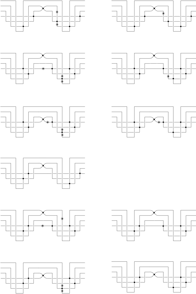
Figure 14. In the diagrams, $*$ denotes a base point. A dot denotes the specified crossing is augmented and the augmentation sends the crossing to the label. Here $-/+$(a) denotes a negative/positive crossing where the ruling has configuration (a) and the rest are defined analogously. (This figure is taken from [14].)

Define the augmentation $\epsilon:\mathcal{A}(D(\Lambda))\to F$ of the DGA for the dipped diagram $D(\Lambda)$ on generators as follows: If the ruling is switched at a crossing $a_{\ell}$, then set $\epsilon(a_{\ell})=1$. If not, set $\epsilon(a_{\ell})=0$. (Note that we can augment the switched crossings to any nonzero element of $F$ and still get an augmentation. But in the case where $\Lambda$ is a knot, by augmenting the switched crossing to $1$, we will be able to ensure $\epsilon(t)=-1$.) Add base points and augment the crossings in the dips following Figure 14. On the remaining generators, set

$$\epsilon(c^{\ell}_{ij})=\begin{cases}1&\text{if }\ell=0\text{ and strands }i,j\text{ are paired in the normal ruling and go through the }p\text{-th }1\text{-handle}\\ (-1)^{\lvert c^{\ell}_{ij}\rvert}&\text{if }\ell=1,i>j,\text{ and strands }i,j\text{ are paired in the normal ruling and go through the }p\text{-th }1\text{-handle}\\ 0&\text{otherwise}.\end{cases}$$

Augment all base points to $-1$.

By considering Figure 14, one can check that $\epsilon$ is an augmentation on the $a_{\ell}$ and the crossings in the dips.

Notation 5.1.

$c^{\ell}_{\{ij\}}=c^{\ell}_{\min(i,j),\max(i,j)}$

We will now check that $\epsilon$ is an augmentation on the $c^{\ell}_{ij}$ generators from the $p$-th $1$-handle.

($\epsilon\partial c^{0}_{ij}=0$) For any ruling, at the left end of the diagram, each strand is paired with another strand going through the same $1$-handle. So for each strand $i$ going through the $p$-th $1$-handle, there exists a strand $j\neq i$ such that strand $i$ and $j$ are paired and $1\leq i,j\leq N_{p}$. So if $i<j$, then $\epsilon(c^{0}_{ij})=1$, $\epsilon(c^{0}_{\{i\ell\}})=0$ for all $\ell\neq j$, and $\epsilon(c^{0}_{\{j\ell\}})=0$ for all $\ell\neq i$. Suppose $i<r<\ell$. We see that $\epsilon(c^{0}_{ir})=0$ if $r\neq j$ and $\epsilon(c^{0}_{r\ell})=0$ if $r=j$. Thus $\epsilon(c^{0}_{ir}c^{0}_{r\ell})=0$ for all $i<r<\ell$ and so

$$\epsilon\partial c^{0}_{i\ell}=\sum_{i<r<\ell}(-1)^{\lvert c^{0}_{ir}\rvert+1}\epsilon(c^{0}_{ir}c^{0}_{r\ell})=0$$

for $i<\ell$.

($\epsilon\partial c^{1}_{ij}=0$) Recall that in the $p$-th $1$-handle

$$\partial c^{1}_{ij}=\delta_{ij}+\sum_{i<\ell\leq N_{p}}(-1)^{\lvert c^{0}_{i\ell}\rvert+1}c^{0}_{i\ell}c^{1}_{\ell j}+\sum_{1\leq\ell<j}(-1)^{\lvert c^{1}_{i\ell}\rvert+1}c^{1}_{i\ell}c^{0}_{\ell j}.$$

If $i\neq j$, then $\epsilon(c^{0}_{i\ell}c^{1}_{\ell j})=0$ and $\epsilon(c^{1}_{i\ell}c^{0}_{\ell j})=0$ for all $\ell$ since it is not possible for strand $i$ to be paired with strand $\ell$ and for strand $\ell$ to be paired with strand $j$ when $i\neq j$. Thus

$$\epsilon\partial c^{1}_{ij}=\sum_{i<\ell\leq N_{p}}(-1)^{\lvert c^{0}_{i\ell}\rvert+1}\epsilon(c^{0}_{i\ell}c^{1}_{\ell j})+\sum_{1\leq\ell<j}(-1)^{\lvert c^{1}_{i\ell}\rvert+1}\epsilon(c^{1}_{i\ell}c^{0}_{\ell j})=0.$$

To show $\epsilon\partial c^{1}_{ii}=0$, suppose strand $i$ is paired with strand $\ell$ through the $p$-th $1$-handle. Then

$$\epsilon\partial c^{1}_{ii} =\begin{cases}1+(-1)^{\lvert c^{0}_{i\ell}\rvert+1}\epsilon(c^{0}_{i\ell}c^{1}_{\ell i})&i<j\\ 1+(-1)^{\lvert c^{1}_{i\ell}\rvert+1}\epsilon(c^{1}_{i\ell}c^{0}_{\ell i})&i>j\end{cases}$$

$$=\begin{cases}1+(-1)^{\lvert c^{0}_{i\ell}\rvert+1}(-1)^{\lvert c^{1}_{\ell i}\rvert}&i<j\\ 1+(-1)^{\lvert c^{1}_{i\ell}\rvert+1}(-1)^{\lvert c^{1}_{i\ell}\rvert}&i>j\end{cases}$$

$$=0$$

by Remark 4.2.

($\epsilon\partial c^{\ell}_{ij}=0$ for $1<\ell$) Recall

$$\partial c^{\ell}_{ij}=\sum_{r=0}^{\ell}\sum_{s=1}^{N_{p}}(-1)^{\lvert c^{r}_{is}\rvert+1}c^{r}_{is}c^{\ell-r}_{sj}$$

for $1<\ell$, $1\leq p\leq k$, and $1\leq i,j\leq N_{p}$. We will show that

$$\epsilon(c^{r}_{is}c^{\ell-r}_{sj})=0,$$

which implies that $\epsilon\partial c^{\ell}_{ij}=0$. If $\ell>2$, then for all $0\leq r\leq\ell$, either $r>1$ or $\ell-r>1$, so $\epsilon(c^{r}_{is}c^{\ell-r}_{sj})=0$ for all $i,j,s$. If $\ell=2$, then $r>1$, $\ell-r>1$, or $r=1=\ell-r$. The first and second case clearly imply $\epsilon(c^{r}_{is}c^{\ell-r}_{sj})=0$. In the final case, this is also clearly true, unless $i=j$ and strands $i$ and $s$ are paired in the ruling. In this case, either $i<s$ or $s<i=j$, so either $\epsilon(c^{1}_{is})=0$ or $\epsilon(c^{1}_{sj})=0$. So

$$\epsilon\partial c^{\ell}_{ii}=\sum_{r=0}^{\ell}\sum_{s=1}^{N_{p}}(-1)^{\lvert c^{r}_{is}\rvert+1}\epsilon(c^{r}_{is}c^{\ell-r}_{si})=0$$

for all $1\leq p\leq k$, $1\leq i\leq N_{p}$, and $\ell>1$. So for $1<\ell$

$$\epsilon\partial c^{\ell}_{ij}=0.$$

(grading) From the definition, $a_{i}$ is augmented only if the $\rho$-graded normal ruling is switched at $a_{i}$ and thus $\rho\big{|}\lvert a_{i}\rvert$. Since $\lvert a_{i}\rvert=\lvert\tilde{a}_{i}\rvert$, the augmentation is $\rho$-graded.

Proposition 5.2.

If $\Lambda\subset\#^{k}(S^{1}\times S^{2})$ is an $n$-component link, $\rho|2r(\Lambda)$ is even, and $\Lambda$ has a $\rho$-graded normal ruling, then the $\rho$-graded augmentation $\epsilon:\mathcal{A}(\Lambda)\to F$ constructed above sends $t_{1}\cdots t_{s}$ to $(-1)^{n}.$

Thus, if $\Lambda$ is a knot, $\epsilon(t)=-1$ for all even-graded augmentations $\epsilon$.

Proof.

Given a $\rho$-graded ruling of $\Lambda$ in $\#^{k}(S^{1}\times S^{2})$, there is a unique way to extend it to a ruling of $S(\Lambda)$ by switching at $d_{ji},e_{ij},f_{ji},g_{ij},h_{ji},q_{ij}$ if and only if strands $i<j$ are paired in the ruling of $\Lambda$. Let $\tilde{\epsilon}:\mathcal{A}(\Lambda)\to F$ be the $\rho$-graded augmentation resulting from the $\rho$-graded normal ruling and let $\epsilon:\mathcal{A}(S(\Lambda))\to F$ be the $\rho$-graded augmentation resulting from the $\rho$-graded normal ruling of $S(\Lambda)$ as constructed in [14] in ${\mathbb{R}}^{3}$. Note that

$$\frac{\epsilon(t_{1}\cdots t_{s})}{\tilde{\epsilon}(t_{1}\cdots t_{s})}=\left(\prod_{1\leq p\leq k}(-1)^{3N_{p}}\right)\prod_{i,j\text{ paired}}(-1)^{6}.$$

If strands $i<j$ are paired near $x=0$ in the ruling of $\Lambda$, then the ruling of $S(\Lambda)$ must be switched at $d_{ji},e_{ij},f_{ji},g_{ij},h_{ji},$ and $q_{ij}$ with configuration $+$(a) since the ruling is $\rho$-graded and $\rho$ is even. So there is one additional base point augmented to $-1$ per crossing. Thus, there are six additional base points augmented to $-1$ for each pair of strands. Each right cusp contributes one extra base point augmented to $-1$ and there are three additional right cusps for each strand. However, $N_{p}$ is even for all $1\leq p\leq k$ by Corollary 4.3 and $\epsilon(t_{1}\cdots t_{s})=(-1)^{n}$ by Theorem 1.1 in [14] so we see that

$$\frac{(-1)^{n}}{\tilde{\epsilon}(t_{1}\cdots t_{s})}=1$$

and so $\tilde{\epsilon}(t_{1}\cdots t_{s})=(-1)^{n}.$

∎

6. Correspondence for links in $J^{1}(S^{1})$

Recall that the $1$-jet space of the circle, $J^{1}(S^{1})$, is diffeomorphic to the solid torus $S^{1}_{x}\times{\mathbb{R}}^{2}_{y,z}$ with contact structure given by $\xi={\hbox{ker}}\,(dz-ydx)$. As in [17], by viewing $S^{1}$ as a quotient of the unit interval, $S^{1}=[0,1]/(0\sim 1)$, we can see Legendrian links in $J^{1}(S^{1})$ as quotients of arcs in $I\times{\mathbb{R}}^{2}$ with boundary conditions which are everywhere tangent to the contact planes. Given a Legendrian link $\Lambda\subset J^{1}(S^{1})$ we will use the methods of Lavrov-Rutherford in [13] to show the following, restated from the introduction:

Theorem 1.5.

Let $\Lambda$ be a Legendrian link in $J^{1}(S^{1})$. Given a field $F$, the Chekanov-Eliashberg DGA $(\mathcal{A},\partial)$ over ${\mathbb{Z}}[t_{1}^{\pm 1},\ldots,t_{s}^{\pm 1}]$ has a $\rho$-graded augmentation $\epsilon:\mathcal{A}\to F$ if and only if a front diagram of $\Lambda$ has a $\rho$-graded generalized normal ruling.

We recall the definition of generalized normal ruling as given in [13].

Definition 6.1.

A generalized normal ruling is a sequence of involutions $\sigma=(\sigma_{1},\ldots,\sigma_{M})$ as in Definition 2.11 with the following differences:

1. Remove the requirement that $\sigma_{m}$ is fixed-point-free and the condition about $1$-handles.

2. If strands $\ell$ and $\ell+1$ cross in the interval $(x_{m-1},x_{m})$ above $I_{m-1}$, where exactly one of the crossing strands is a fixed point of $\sigma_{m}$, then the crossing is a switch if $\sigma_{m}$ satisfies the conditions in (3) of Definition 2.11. If crossing is a switch, then we require an additional normality condition:

   $$\sigma_{m}(\ell)=\ell<\ell+1<\sigma_{m}(\ell+1)\text{ or }\sigma_{m}(\ell)<\ell<\ell+1=\sigma_{m}(\ell+1).$$

A strictly generalized normal ruling is a generalized normal ruling which is not a normal ruling, in other words, a generalized normal ruling with at least one fixed point.

Thus, near a crossing, a generalized normal ruling looks like the crossings in Figure 7 or Figure 15.

2pt $(g)$ [t] at 89 10 $(h)$ [t] at 317 10

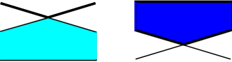
Figure 15. These figures give the configuration of a generalized normal ruling near a switched crossing involving exactly one self-paired strand. With the top row of configurations in Figure 7, these are all possible configurations of a generalized normal ruling near a switched crossing.

Remark 6.2.

1. If a crossing involving strands $\ell$ and $\ell+1$ occurs in the interval $(x_{m-1},x_{m})$ and both crossing strands are fixed by the ruling, self-paired, in other words, $\sigma_{m-1}(\ell)=\ell$ and $\sigma_{m-1}(\ell+1)=\ell+1$, then $\sigma_{m}=(\ell\quad\ell+1)\circ\sigma_{m-1}\circ(\ell\quad\ell+1)$ and so we will not consider such crossings to be switched.

2. Note that the number of generalized normal rulings of a Legendrian link is not invariant under Legendrian isotopy.

The definition of the Chekanov-Eliashberg DGA of a Legendrian link in ${\mathbb{R}}^{3}$ can be extended to Legendrian links in $J^{1}(S^{1})$. (One can find the full definition of the Chekanov-Eliashberg DGA of a Legendrian link in $J^{1}(S^{1})$ in [17].) Note that given an augmentation of the Chekanov-Eliashberg DGA over ${\mathbb{Z}}[t,t^{-1}]$ of a Legendrian link in $S^{1}\times S^{2}$, one can define an augmentation of the DGA of the analogous link (where if a strand goes through the $1$-handle with $y=y_{0}$ at $x=0$, then it is paired with the strand going through the $1$-handle with $y=y_{0}$ at $x=A$) in $J^{1}(S^{1})$ and similarly for normal rulings. (The resulting normal ruling of the link in $J^{1}(S^{1})$ will not have any self-paired strands.) However, there is no reason to think the converse is true.

6.1. Matrix definition of the DGA in $J^{1}(S^{1})$

Ng and Traynor define a version of the Chekanov-Eliashberg DGA $\mathcal{A}$ over $R={\mathbb{Z}}[t,t^{-1}]$ in [17]. For ease of definition, note that we can assume all left and right cusps involve the two strands with lowest $z$-coordinate (and thus highest labels) and that there is one base point at $x=0$ on each strand and these are the only base points. We give the definition of the DGA for the dipped version $\Lambda$, $D(\Lambda)$ as in [13]. Label the dips as in Figure 13 with $b^{m}_{ij}$ and $c^{m}_{ij}$ in the dip at $x_{m}$. Place these generators in upper triangular matrices

$$B_{m}=(b^{m}_{ij})\text{ and }C_{m}=(c^{m}_{ij}).$$

Note that since the $x$-coordinate is $S^{1}$-valued, we need to add the convention that $B_{0}=B_{M}$ and $C_{0}=C_{M}$. We then see that

$$\partial C_{m} =(\Sigma C_{m})^{2},$$

$$\partial B_{m} =-\Sigma(I+B_{m})\Sigma C_{m}+\widetilde{C}_{m-1}(I+B_{m}),$$

where $\Sigma$ is the diagonal matrix with $(-1)^{\mu_{m}(i)}$ the $i$-th entry on the diagonal for Maslov potential $\mu_{m}$ at $x=x_{m}$ and $I$ is the appropriately sized identity matrix. The form of $\widetilde{C}_{m}$ will depend on the tangle appearing in the interval $(x_{m-1},x_{m})$.

If $(x_{m-1},x_{m})$ contains a crossing $a_{m}$ of strands $k$ and $k+1$, then

$$\partial a_{m}=c^{m-1}_{k,k+1}$$

$$\widetilde{C}_{m-1}=U_{k,k+1}\widehat{C}_{m-1}V_{k,k+1},$$

where $U_{k,k+1}$ and $V_{k,k+1}$ are the identity matrix with the $2\times 2$ block in rows $k$ and $k+1$ and columns $k$ and $k+1$ replaced with $\begin{pmatrix}0&1\\ 1&(-1)^{\lvert a_{m}\rvert+1}a_{m}\end{pmatrix}$ for $U_{k,k+1}$ and $\begin{pmatrix}a_{m}&1\\ 1&0\end{pmatrix}$ for $V_{k,k+1}$, and $\widehat{C}_{m-1}$ is $C_{m-1}$ with $0$ replacing the entry $c^{m-1}_{k,k+1}$.

If $(x_{m-1},x_{m})$ contains a left cusp, by assumption strands $N(m)-1$ and $N(m)$ are incident to the cusp. In this case,

$$\widetilde{C}_{m-1}=JC_{m-1}J^{T}+W,$$

where $J$ is the $N(m-1)\times N(m-1)$ identity matrix with two rows of zeroes added to the bottom and $W$ is $N(m)\times N(m)$ matrix where the $(N(m)-1,N(m))$-entry is $1$ and all other entries are zero.

Finally, if $(x_{m-1},x_{m})$ contains a right cusp $a_{m}$, by assumption strands $N(m)-1$ and $N(m)$ are incident to the cusp. In this case

$$\partial a_{m}=1+c^{m-1}_{N(m-1)-1,N(M-1))},$$

$$\widetilde{C}_{m-1}=KC_{m-1}K^{T},$$

where $K$ is the $N(m-1)\times N(m-1)$ identity matrix with two columns of zeroes added to the right.

6.2. Proof of correspondence

We will use the methods of [13] to prove Theorem 1.3. A few conventions and notation: Assume all left and right cusps occur at lowest $z$-coordinate of all strands at that $x$-coordinate, in other words, assume for all cusps that the two strands with highest label are incident to the cusp. Assume that there is one base point at $x=0$ of $\Lambda$ on each strand and these are the only base points. Given an involution $\sigma$ of $\{1,\ldots,N\}$, $\sigma^{2}=id$, we define $A_{\sigma}=(a_{ij})$ the $N\times N$ matrix with entries

$$a_{ij}=\begin{cases}1&\text{if }i<\sigma(i)=j\\ 0&\text{otherwise}\end{cases}$$

(Ruling to augmentation) Given a generalized normal ruling $\sigma=(\sigma_{1},\ldots,\sigma_{M})$, we will define a $\rho$-graded augmentation $\epsilon:\mathcal{A}(D(\Lambda))\to F$ satisfying Property (R) (as in [18]) by defining $\epsilon$ on the crossings in the dip involving crossings $b^{0}_{ij}$ and $c^{0}_{ij}$ and extending to the right.

Property (R): In any dip, the generator $c^{m}_{rs}$ is augmented (to $1$) if and only if $\sigma_{m}(r)=s$.

Add a base point to the loop in each resolution of a right cusp. Augment all base points to $-1$. Given a crossing $a$, set

$$\epsilon(a)=\begin{cases}1&\text{if the ruling is switched at }a\\ 0&\text{otherwise}.\end{cases}$$

Define $\epsilon(B_{0})=0$ and $\epsilon(C_{0})=A_{\sigma_{0}}$. We will now extend $\epsilon$ to the right. Suppose $\epsilon$ is defined on all crossings in the interval $(0,x_{m-1})$. If $(x_{m-1},x_{m})$ contains a crossing, define $\epsilon$ on crossings $b^{m}_{ij}$ and $c^{m}_{ij}$ and add base points as in Figure 14 and Figure 16. If $(x_{m-1},x_{m})$ contains a left cusp, set

$$\epsilon(B_{m})=J\epsilon(B_{m-1})J^{T}+W.$$

If $(x_{m-1},x_{m})$ contains a right cusp, set

$$\epsilon(B_{m})=K\epsilon(B_{m-1})K^{T}.$$

It is easy to check that by our definition the augmentation satisfies Property (R), which tells us $\epsilon(B_{0})=\epsilon(B_{M})$ and $\epsilon(C_{0})=\epsilon(C_{M})$, and our augmentation is a $\rho$-graded augmentation.

3pt (g) [b] at 217 157 $c$ [tl] at 158 76 $a$ [b] at 217 126 $a^{-1}$ [tr] at 306 45 $ac$ [tl] at 387 77 $1$ [r] at 275 92 $2$ [l] at 306 104

(h) [b] at 699 157 $c$ [tl] at 607 44 $a$ [b] at 699 94 $a^{-1}$ [tr] at 758 77 $ac$ [tl] at 834 44

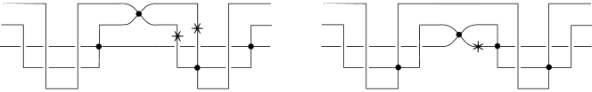
Figure 16. In the diagrams, $*_{i}$ denotes the base point associated to $t_{i}$. A dot denotes the specified crossing is augmented and the augmentation sends the crossing to the label. In configuration (g), $\epsilon(t_{1})=(-1)^{\lvert a\rvert+1}$ and $\epsilon(t_{2})=(-1)^{\lvert c_{i,i+1}\rvert+1}$. In configuration (h), $\epsilon(t)=-1$.

(Augmentation to ruling) This direction of the proof follows that of the ${\mathbb{Z}}/2$ case in [13] and is based on canonical form results from linear algebra due to Barannikov [1].

Definition 6.3.

An $M$-complex $(V,\mathcal{B},d)$ is a vector space $V$ over a field $F$ with an ordered basis $\mathcal{B}=\{v_{1},\ldots,v_{N}\}$ and a differential $d:V\to V$ of the form $dv_{i}=\sum_{j=i+1}^{N}a_{ij}v_{j}$ satisfying $d^{2}=0$.

The following two propositions are essentially Proposition 5.4 and 5.6 in [13] and Lemma 2 and 4 in [1].

Proposition 6.4.

If $(V,\mathcal{B},d)$ is an $M$-complex, then there exists a triangular change of basis $\{\tilde{v}_{1},\ldots,\tilde{v}_{N}\}$ with $\tilde{v}_{i}=\sum_{j=1}^{N}a_{ij}v_{j}$ and an involution $\tau:\{1,\ldots,N\}\to\{1,\ldots,N\}$ such that

$$d\tilde{v}_{i}=\begin{cases}\tilde{v}_{j}&\text{if }i<\tau(i)=j,\\ 0&\text{otherwise}.\end{cases}$$

Moreover, the involution $\tau$ is unique.

Remark 6.5.

1. If the basis elements $v_{i}$ have been assigned degrees $\lvert v_{i}\rvert\in{\mathbb{Z}}/\rho$ such that $V$ is ${\mathbb{Z}}/\rho$-graded and $d$ has degree $-1$, then it can be assumed that the change of basis preserves degree. Thus, if $i<\tau(i)=j$, then $\lvert v_{i}\rvert=\lvert v_{j}\rvert+1$.

2. The set $\{[\tilde{v}_{i}]:\tau(i)=i\}$ forms a basis for the homology $H(V,d)$.

3. In matrix formulation, Proposition 6.4 says there is a unique function $D\mapsto\tau(D)$ which assigns an involution $\tau=\tau(D)$ to each strictly upper triangular matrix $D$ with $D^{2}=0$ and there is an invertible upper triangular matrix $P$ so that $PDP^{-1}=A_{\tau}$. The uniqueness statement tells us that $\tau(QDQ^{-1})=\tau(D)$ if $Q$ is a nonsingular upper triangular matrix.

Proposition 6.6.

Suppose $(V,\mathcal{B},d)$ is an $M$-complex and $k\in\{1,\ldots,N\}$ such that $dv_{k}=\sum_{j=k+2}^{N}a_{kj}v_{j}$ so the triple $(V,\mathcal{B}^{\prime},d)$ with $\mathcal{B}^{\prime}=\{v_{1},\ldots,v_{k+1},v_{k},\ldots,v_{N}\}$ is also an $M$-complex. Then the associated involutions $\tau$ and $\tau^{\prime}$ from Proposition 6.4 are related as follows:

1. If

   $$\tau(k+1)<\tau(k)<k<k+1,$$

   $$\tau(k)<k<k+1<\tau(k+1),$$

   $$k<k+1<\tau(k+1)<\tau(k),$$

   $$\tau(k)<k<k+1=\tau(k+1),$$

   $$\tau(k)=k<k+1<\tau(k+1)$$

   then either $\tau^{\prime}=\tau$ or $\tau^{\prime}=(k\quad k+1)\circ\tau\circ(k\quad k+1)$.

2. Otherwise $\tau^{\prime}=(k\quad k+1)\circ\tau\circ(k\quad k+1)$.

(Augmentation to ruling) This part of the proof is the same as the analogous statement in [13] with $\Sigma\epsilon(C_{m-1})$ replacing $\epsilon(Y_{m-1})$.

6.3. Corollaries

The following proposition uses techniques in the proof of Theorem 1.5 to show that

$$\operatorname{Aug}_{\rho}(\Lambda)=F\backslash 0$$

for any field $F$ and any $\rho$ if $\Lambda$ has a strictly generalized normal ruling.

Proposition 6.7.

Given a field $F$ and a Legendrian link $\Lambda\subset J^{1}(S^{1})$ with $n$ components and a strictly generalized normal ruling, for all $0\neq x\in F$ there exists an augmentation $\epsilon:\mathcal{A}\to F$ such that

$$\epsilon(t_{1}\cdots t_{s})=x.$$

Proof.

Fix $0\neq x\in F$. Given a generalized normal ruling $\sigma=(\sigma_{1},\ldots,\sigma_{M})$ for $\Lambda$ with a self-paired strand, we will construct an augmentation $\epsilon:\mathcal{A}(D(\Lambda))\to F$ such that $\epsilon(t_{1}\cdots t_{s})=x$.

Suppose $k$ is the label at $x=0$ of a self-paired strand of the generalized normal ruling $\sigma$, in other words, $\sigma_{0}(k)=k$. We can assume that $D(\Lambda)$ has one base point corresponding to $t_{i}$ on strand $i$ at $x=0$ and one base point in the loop in the resolution of each right cusp, and no other base points. Define

$$\epsilon(t_{i})=\begin{cases}(-1)^{N+c-1}x&\text{if }i=k,\\ -1&\text{otherwise},\end{cases}$$

where $c$ is the number of right cusps and $N$ is the number of strands at $x=0$.

Define $\epsilon$ on all crossings as in the proof of ruling to augmentation in Theorem 1.5. Note that $t_{k}$ does not appear on the boundary of any totally augmented disks and so $\epsilon$ is still an augmentation, but now

$$\epsilon(t_{1}\cdots t_{s})=x$$

as desired. ∎

Remark 6.8.

For any link $\Lambda\subset J^{1}(S^{1})$, one can consider the analogous link $\Lambda^{\prime}\subset S^{1}\times S^{2}$. Note that $\mathcal{A}(\Lambda)\to\mathcal{A}(\Lambda^{\prime})$ where the map is inclusion. Thus, any augmentation $\epsilon^{\prime}:\Lambda^{\prime}\to F$ gives an augmentation $\epsilon:\Lambda\to F$. As one would expect from Theorem 1.3 and Theorem 1.5, it is also clear that any normal ruling of $\Lambda^{\prime}\subset S^{1}\times S^{2}$ gives a generalized normal ruling of $\Lambda\subset J^{1}(S^{1})$.

Appendix

The appendix will address Corollary 1.4 which follows from

1. Theorem 1.3 over ${\mathbb{Q}}$ and

2. the result that if a graded augmentation to the rationals exists then the full symplectic homology is nonzero.

The second result is known to experts. We will outline the proof here for completeness. Statement 2 is a straight forward consequence of work of Bourgeois, Ekholm, and Eliashberg [2] and has previously been observed in [15].

Every connected Weinstein (Stein) $4$-manifold $X$ can be decomposed into $1$- and $2$-handle attachments to $D^{4}$ along $\partial D^{4}=S^{3}$. Thus, for each such $4$-manifold there exists a Legendrian link $\Lambda$ in $\#^{k}(S^{1}\times S^{2})$, the boundary of the $4$-manifold, so that attaching $2$-handles along $\Lambda$ to $\#^{k}(S^{1}\times S^{2})$ results in $X$.

Using the notation of [2], results of Bourgeois, Ekholm, and Eliashberg in [2] tell us that:

Proposition 6.9 ([2] Corollary 5.7).

$$S\mathbb{H}(X)=L\mathbb{H}^{Ho}(\Lambda),$$

where $L\mathbb{H}^{Ho}(\Lambda)$ is the homology of the Hochschild complex associated to the Chekanov-Eliashberg differential graded algebra over ${\mathbb{Q}}$.

Therefore, if the DGA for $\Lambda$ has a graded augmentation to ${\mathbb{Q}}$, then $S\mathbb{H}(X)$ is nonzero. By Theorem 1.3, we know that the DGA for $\Lambda$ has a graded augmentation to ${\mathbb{Q}}$ if and only if $\Lambda$ has a graded normal ruling. Thus, restated from the introduction:

Corollary 1.4.

If $X$ is the Weinstein $4$-manifold that results from attaching $2$-handles along a Legendrian link $\Lambda$ to $\#^{k}(S^{1}\times S^{2})$ and $\Lambda$ has a graded normal ruling, then the full symplectic homology $S\mathbb{H}(X)$ is nonzero.

For completeness, we give an outline of the proof of statement 2. Recall that full symplectic homology is a symplectic invariant of Weinstein $4$-manifolds which coincides with the Floer-Hofer symplectic homology.

We will show that given a graded augmentation $\epsilon^{\prime}$ of the Chekanov-Eliashberg DGA over ${\mathbb{Z}}[t,t^{-1}]$ of a Legendrian knot $\Lambda$ to ${\mathbb{Q}}$, one can define a graded augmentation $\epsilon:LH^{Ho}(\Lambda)\to{\mathbb{Q}}$, where the homology of $LH^{Ho}(\Lambda)$ is $L\mathbb{H}^{Ho}(\Lambda)$. Recall that elements of $LH^{Ho}(\Lambda)=\widecheck{LHO^{+}}(\Lambda)\oplus{\mathbb{Q}}\oplus\widehat{LHO^{+}}(\Lambda)$ are of the form $(\check{w},n,\hat{v})$ for some $w,v\in LHO(\Lambda)\subset LHA(\Lambda)$ and $n\in{\mathbb{Q}}$. Define

$$\epsilon:LH^{Ho}(\Lambda)=\widecheck{LHO^{+}}(\Lambda)\oplus{\mathbb{Q}}\oplus\widehat{LHO^{+}}(\Lambda)\to{\mathbb{Q}}$$

$$\epsilon(\check{w},n,\hat{v})=\epsilon^{\prime}(w)+n$$

Let us check that this gives an augmentation. Recall

$$d_{H_{0}}(\check{w},n,\hat{v})=(\check{d}_{LHO^{+}}\check{w}+d_{MH_{0}^{+}}\hat{v},n,\hat{d}_{LHO^{+}}\hat{v})=\left(\sum_{j=1}^{r}\check{w}_{j}+\check{c}_{1}c_{2}\cdots c_{\ell}-c_{1}\cdots c_{\ell-1}\check{c}_{\ell},n,\hat{d}_{LHO^{+}}\hat{v}\right)$$

if $d_{LHO^{+}}(w)=\sum_{j=1}^{r}w_{j}$ and $v=c_{1}\ldots c_{\ell}$. Thus,

$$\epsilon(d_{H_{0}}(\check{w},n,\hat{v})) =\epsilon^{\prime}\left(\sum_{j=1}^{r}w_{j}\right)+\epsilon^{\prime}(c_{1}\cdots c_{\ell})-\epsilon^{\prime}(c_{1}\cdots c_{\ell})+n$$

$$=\epsilon^{\prime}\left(\sum_{j=1}^{r}w_{j}+n\right)$$

$$=\epsilon^{\prime}(d_{LHO}w)=0$$

since $\epsilon^{\prime}$ is an augmentation of $LHA(\Lambda)$, $LHO(\Lambda)\subset LHA(\Lambda)$, and $d_{LHO}=d_{LHA}|_{LHO}$.

One can show that this construction also works if $\epsilon^{\prime}$ is a pure augmentation of a link $\Lambda=\Lambda_{1}\coprod\cdots\coprod\Lambda_{N}$, where an augmentation is pure if when a crossing $c$ is augmented, then there exists $1\leq i\leq N$ such that $c$ is a crossing of $\Lambda_{i}$.

References

- [1] S. A. Barannikov. The framed Morse complex and its invariants. In Singularities and bifurcations, volume 21 of Adv. Soviet Math., pages 93–115. Amer. Math. Soc., Providence, RI, 1994.
- [2] Frédéric Bourgeois, Tobias Ekholm, and Yasha Eliashberg. Effect of Legendrian surgery. Geom. Topol., 16(1):301–389, 2012. With an appendix by Sheel Ganatra and Maksim Maydanskiy.
- [3] Yu. V. Chekanov and P. E. Pushkar′. Combinatorics of fronts of Legendrian links, and Arnol′d’s 4-conjectures. Uspekhi Mat. Nauk, 60(1(361)):99–154, 2005.
- [4] Yuri Chekanov. Differential algebra of Legendrian links. Invent. Math., 150(3):441–483, 2002.
- [5] Tobias Ekholm and Lenhard Ng. Legendrian contact homology in the boundary of a subcritical Weinstein 4-manifold. J. Differential Geom., 101(1):67–157, 2015.
- [6] Ya. M. Eliashberg. A theorem on the structure of wave fronts and its application in symplectic topology. Funktsional. Anal. i Prilozhen., 21(3):65–72, 96, 1987.
- [7] Yakov Eliashberg. Invariants in contact topology. In Proceedings of the International Congress of Mathematicians, Vol. II (Berlin, 1998), number Extra Vol. II, pages 327–338, 1998.
- [8] John B. Etnyre. Legendrian and transversal knots. In Handbook of knot theory, pages 105–185. Elsevier B. V., Amsterdam, 2005.
- [9] John B. Etnyre, Lenhard L. Ng, and Joshua M. Sabloff. Invariants of Legendrian knots and coherent orientations. J. Symplectic Geom., 1(2):321–367, 2002.
- [10] Dmitry Fuchs. Chekanov-Eliashberg invariant of Legendrian knots: existence of augmentations. J. Geom. Phys., 47(1):43–65, 2003.
- [11] Dmitry Fuchs and Tigran Ishkhanov. Invariants of Legendrian knots and decompositions of front diagrams. Mosc. Math. J., 4(3):707–717, 783, 2004.
- [12] Robert E. Gompf. Handlebody construction of Stein surfaces. Ann. of Math. (2), 148(2):619–693, 1998.
- [13] Mikhail Lavrov and Dan Rutherford. Generalized normal rulings and invariants of Legendrian solid torus links. Pacific J. Math., 258(2):393–420, 2012.
- [14] Caitlin Leverson. Augmentations and rulings of Legendrian knots. To appear in J. Symplectic Geom., 2014. http://arxiv.org/abs/1403.4982.
- [15] Tye Lidman and Steven Sivek. Contact structures and reducible surgeries. 2014. http://arxiv.org/abs/1410.0303.
- [16] Lenhard Ng and Daniel Rutherford. Satellites of Legendrian knots and representations of the Chekanov–Eliashberg algebra. Algebr. Geom. Topol., 13(5):3047–3097, 2013.
- [17] Lenhard Ng and Lisa Traynor. Legendrian solid-torus links. J. Symplectic Geom., 2(3):411–443, 2004.
- [18] Joshua M. Sabloff. Augmentations and rulings of Legendrian knots. Int. Math. Res. Not., (19):1157–1180, 2005.