Periodic modulation in pulse arrival times from young pulsars: a renewed case for neutron star precession

Abstract

In a search for periodic variation in the arrival times of pulses from 151 young, energetic pulsars, we have identified seven cases of modulation consistent with one or two harmonics of a single fundamental with time-scale 0.5–1.5 yr. We use simulations to show that these modulations are statistically significant and of high quality (sinusoidal) even when contaminated by the strong stochastic timing noise common to young pulsars. Although planetary companions could induce such modulation, the large implied masses and 2:1 mean motion resonances challenge such an explanation. Instead, the modulation is likely to be intrinsic to the pulsar, arising from quasi-periodic switching between stable magnetospheric states, and we propose that precession of the neutron star may regulate this switching.

1 Introduction

In the tour de force publication announcing the discovery of pulsars, Hewish et al. (1968) made the first use of periodic modulation of the pulse time of arrival (TOA), induced by the earth’s motion around the sun, to pinpoint the position of PSR B1919$+$21. The study of TOA modulation has ever since been the heart of pulsar science. After astrometry, the most common manifestation of modulation arises from the reflex motion induced by a companion, notably leading to the discoveries of the relativistic double neutron star system B1913$+$16 (Hulse & Taylor, 1975) and the first exoplanets orbiting PSR B1257+12 (Wolszczan & Frail, 1992).

Later, Stairs, Lyne & Shemar (2000) reported quasi-periodic modulation of the TOAs of PSR B1828$-$11 (PSR J1830$-$1059) which was correlated with changes in the pulse shape and proposed free precession of the neutron star as a natural explanation of these observations. In brief, the precession induces a periodic change in spin-down torque, leading to TOA modulation, and the precessional motion allows the observer to see different portions of the neutron star polar cap, gradually changing the pulse emission profile. Various authors explored the implications for pulsar beam shapes and geometry (e.g. Jones & Andersson, 2001; Link & Epstein, 2001) and for neutron star interiors (e.g. Cutler, Ushomirsky & Link, 2003; Link, 2003).

A decade later, Lyne et al. (2010) identified similar quasi-periodic modulation in 17 pulsars drawn from a sample of 366 pulsars (Hobbs et al., 2010) timed over decades. Six of these pulsars showed correlated profile variation; however, they also observed the pulse profile to oscillate between two distinct shapes on short time-scales. This behaviour suggests that the periodicity is not due to secular motion of the neutron star but to rapid reconfiguration of the pulsar magnetosphere between two spin-down states. Lyne et al. (2010) further argued that state switching with time-scales randomly distributed around a fundamental value could fully explain the observed TOA modulation. Consequently, the precession hypothesis fell out of favour. However, the year-long time-scale underpinning the state switching is difficult to produce from any dynamic process in the pulsar magnetosphere (e.g. Cordes, 2013).

A better understanding of both the magnetospheric switching process and its regularity is hampered by the paucity of such pulsars; even the large parent sample Lyne et al. (2010) produced only 17 examples of TOA modulation, and most of these cases are not of high quality factor. Here, we report the discovery of nearly sinusoidal TOA modulation from seven pulsars drawn from a sample of 151 young, energetic (spin-down power $\dot{E}>10^{34}$ erg s^-1) pulsars. The short spin periods are complementary to the sample of Lyne et al. (2010) and offer the opportunity to study the modulation period $P_{m}$ over a broad range of pulsar ages and spin periods $P_{s}$. Combined measurements of $P_{m}$ from other neutron stars (Jones, 2012), we find a strong correlation between $P_{m}$ and $P_{s}$, a scaling that can be readily explained if neutron star precession drives the “switching clock”. However, as we discuss below, many difficulties with such a mechanism remain.

Below, we outline our search for periodic modulations and the resulting candidates (§2). The identification of these signals is complicated by “timing noise”, and in §3 we detail the simulations we perform to verify and characterise the candidates. In §4, we search for variations in the pulse profile of our candidate but find no strong evidence for them. Finally, we discuss in §5 the possible causes of the TOA modulation, including planetary companions and a hybrid scenario of magnetospheric switching with free precession.

2 Search for Periodic Signals

Our sample of 151 pulsars, the data (raw and reduced), the maximum likelihood method of analysis, and the search for periodic signals (in the context of upper limits on planetary companions) are described fully in Kerr et al. (2015). For completeness, we summarise this discussion and review the search for quasi-periodic signals.

The TOAs are modelled as a parametric “spin-down” process which we evaluate with tempo2 (Hobbs, Edwards & Manchester, 2006). To the residuals of this model are added components of white noise—both measurement (radiometer) and “jitter” noise (Shannon et al., 2014))—and strong, red “timing” noise which we model as a widesense stationary process whose spectrum is described by a power law with a low-frequency cutoff (Coles et al., 2011):

$$P(f)=A_{0}\left[1+(f/f_{c})^{2}\right]^{-\alpha/2}.$$ (1)

These noise components manifest as the diagonal and non-diagonal components of a covariance matrix for the residuals, $C$, which allows evaluation of the Gaussian log likelihood for the full (spin-down plus noise) model. We use Monte Carlo Markov Chains methods, in particular the emcee package (Foreman-Mackey et al., 2013), to evaluate the likelihood and characterize its shape, allowing parameter inference.

To search for harmonic modulation, we simply add a sinusoid with arbitrary amplitude and phase to the spin-down model and compare the change in log likelihood $\delta\log\mathcal{L}$ between the two best-fitting models. The significance of a given value of $\delta\log\mathcal{L}$ will generally depend on the particular noise characteristics of a pulsar, but metrics like the Akaike information criterion suggest that values of $\delta\log\mathcal{L}>6$ are significant for three degrees of freedom. Because we also have a sample of 151 pulsars, or “trials”, we adopt $\delta\log\mathcal{L}>10$, for any trial harmonic frequency, as a threshold for further consideration of a pulsar as a modulation candidate.

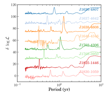
Figure 1: The change in log likelihood ($\delta\log\mathcal{L}$) between a model with and without a single sinusoidal modulation at the indicated period, with an arbitrary vertical offset of $\delta\log\mathcal{L}=15$ between pulsars for clarity.

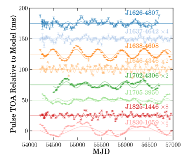
Figure 2: The deviation in arrival times of pulses from the indicated pulsars relative to a simple timing model including a cubic term. Due to the higher level of red noise, we have additionally removed a series of six sinusoids (PSRs J1637$-$4642 and J1825$-$1446) and eight sinusoids (PSR J1646$-$4346). We note that these frequencies are substantially lower than the detected modulation frequencies. For clarity, the residuals are connected by a dashed line and have been multiplied by the indicated factor to ease comparison. The best-fit single-sinusoid model is indicated by the solid line.

The $\delta\log\mathcal{L}$ for the eight pulsars surpassing this threshold, as a function of trial harmonic modulation period, appears in Figure 1, which can be thought of as a periodogram that properly accounts for the red noise. In such a periodogram, representation of a pure sinusoid as a Dirac $\delta$ function is modified by the “window function”, determined by the length, cadence, and noise properties of the data for a given pulsar. The window function is not known a priori, but with the exception of PSR B1828$-$11, the widths of the peaks are generally consistent with signals caused by sinusoidal modulation. We verify this below with simulations. A clear second harmonic, whose significance and nature we also explore below, is present in some pulsars.

The timing residuals to simple spin-down models that remove low frequency timing noise appear in Figure 2. The quasi-periodic oscillation is evident to the eye in most. Anecdotally, our threshold of $\delta\log\mathcal{L}>10$ seems to reproduce what the eye picks up in the time domain. It seems likely, then, that there are additional pulsars harbouring such signals that fail to rise above the noise in our analysis. Moreover, pulsars like PSR B1828$-$11, with multiple time-scales, are not well modelled by our single-frequency test, yielding lower significances. However, searches for multiple sinusoids are computationally prohibitive, and we have visually examined the timing residuals for all 151 pulsars to search for any additional “obvious” modulation, finding none. As noted by Kerr (2015), the presence of strong timing noise causes sensitivity to coherent sinusoids to scale roughly as the square root of observing span. Thus, for most of our sample, substantial further observations will be required to detect modulations with lower amplitude.

3 Characterisation of periodic signals

Characterising periodicity in astronomical signals is a common yet often challenging task. One might, e.g., search for peaks in the time series power spectrum, but nonuniform observing cadence and sensitivity (e.g. due to changes in source brightness) hamper simple interpretations of spectral features. This difficulty is encapsulated in the “window function” and the well-known convolution theorem. Observing with nonuniform cadence and sensitivity is equivalent to multiplying the true signal by a complicated weighting window function. The simplest window function, a top hat, is Fourier transformed into a sinc; thus, the power spectrum of a finite-length time series will be convolved with a function that diminishes asymptotically as $f^{-2}$. This effect, which blurs spectral features and, for steep spectra, shifts low frequency power to high frequencies, is known as spectral leakage.

Our data have nonuniform cadence and hetereogeneous sensitivity (due to system evolution and varying source brightness) and are affected by timing noise with a steep red spectrum. While we can mitigate spectral leakage following the methods of Coles et al. (2011), the quasi-sinusoidal signals in the data are sufficiently strong that they bias the measurement of the timing noise parameters. These considerations rule out spectral analysis as a primary method for identifying and characterising modulations in our data; instead, we outline below a prescription of simulations to cleanly separate the effects of timing noise and sinusoidal modulation. We conclude the section with a discussion of two pulsars, B1828$-$11 and B0740$-$28, whose spectral features indicate strong modulation but which our analysis is able to show are of lower quality.

3.1 Simulations

To quantify both the significance and the quality factor of the periodic modulation, we generated a series of simulated realizations of our TOAs. For our control case (S0), we adopted a red-noise model similar to that observed in the data after removing the apparent sinusoidal modulation. We next generated two additional sets of simulations with the same red-noise model plus a single sinusoid (S1) and two sinusoids (S2); we only performed S2 for those pulsars with evidence of a harmonic. The observed and simulated parameters appear in Table 1. In the table, we do not report the measured values of the spin noise parameters as they are typically covariant. Instead, we have chosen representative values that both yield the correct value for the likelihood (discussed below) and reproduce the observed spectrum of the time series residuals. To form each of 100 realizations, we used the original TOA sampling and a simple timing solution to generate an “idealized” set of TOAs. To these we added white noise from measurement error and “jitter”, the latter at the values determined from a model of the data. To these white-noise realizations, we added a random time series with a spectrum matching the red-noise model.

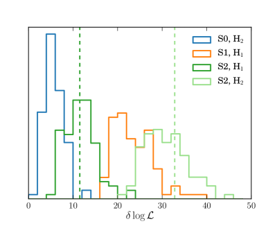
Figure 3: Distributions of the change in $\log$ likelhihood for the simulations of PSR J1705$-$3950 described in the main text; all values are relative to $\log\mathcal{L}(H_{0})$ for the indicated simulation. The observed values $\delta\log\mathcal{L}=11.5$ and $\delta\log\mathcal{L}=32.8$ are shown with vertical dashed lines.

For each set of simulations, we followed the same method as for the real data and determined best-fit parameters under each of the three hypotheses: $H_{0}$, no sinusoids; $H_{1}$, a single sinusoid; and $H_{2}$, two sinusoids. We then compared the change in the log likelihood, $\delta\log\mathcal{L}$, as a measure of both significance and goodness of fit. The permutations of $S$ and $H$ allow a variety of statistical tests. E.g., the distribution of $\log\mathcal{L}(H_{2})-\log\mathcal{L}(H_{0})$ using data from S0 allows us to test how often noise fluctuations produce large values of $\delta\log\mathcal{L}$ by chance when we search for two sinusoids.

As an example, we consider the pulsar with the strongest and most complex modulation, PSR J1705$-$3950, which has evidence for a second harmonic. The distributions of $\delta\log\mathcal{L}$ for some of the permutations of $S$ and $H$ appear in Figure 3. The first distribution (blue in the Figure, leftmost) is a significance test, in which we simulate only red noise (S0) but fit a model with two sinusoids ($H_{2}$); its properties are reported in the rightmost column of Table 2. The realizations of $\delta\log\mathcal{L}$ are all well below the observed value under $H_{2}$, meaning the modulations cannot be produced by noise fluctuations.

The next distribution to the right (green) contains the results for a simulation with two sinusoids (S2) while only one is modelled ($H_{1}$); the values correspond to the middle column and last two rows of the relevant entry in Table 2. This combination tests the consistency of the two-sinusoid model by examining the significance we achieve when we only model part of the modulation, and we see that the observed value of $\delta\log\mathcal{L}(H_{1})=11.5$ lies within the core of the distribution of simulated values, implying consistency of the two-sinusoid simulations with the data.

Next is the distribution for a simulation with only one sinusoid (S1) and the corresponding change in log likelihood under H₁. This distribution is in strong disagreement with the observed value of $\delta\log\mathcal{L}(H_{1})$=11.5. For simplicity of presentation, we have excluded the distribution of $\delta\log\mathcal{L}(H_{2})-\delta\log\mathcal{L}(H_{1})$, which provides the best significance test of the harmonic, but these results are tabulated in the rightmost column of S1 for the relevant pulsars.

Finally, rightmost (light green) is the distribution of $\delta\log\mathcal{L}$ for the scenario we believe describes the data best, viz. two sinusoids. The observed value again lies within the core of the simulated values. This is a key point, both in terms of the significance of the model and in goodness of fit. Not only does the two-sinusoid hypothesis (H₂) produce a $\delta\log\mathcal{L}$ much larger than that produced by chance, but the observed value of $\delta\log\mathcal{L}$ is precisely the same as that observed for the simulations. That is, the data are completely consistent with high quality factor modulations. This test is equivalent to, and arguably better than, jackknife tests where we search for the signal at lower significance in subsets of the data. Perhaps most interestingly, the absolute value of $\log\mathcal{L}$ agrees between the simulations and data. This means that our model completely captures all of the information in the data, such that our assumptions about the noise model, spin-down model, and modulations are correct and complete.

PSR J1705$-$3950 is our best example; its low white and red noise, together the highest ratio of harmonic to fundamental amplitudes in the sample, make it ideal for detecting all of the features. But similar remarks apply to other candidates in various levels of dilution: most lack evidence for a second harmonic, but the data are perfectly consistent with and statistically favour at least one sinusoid. The full results of the simulations are compiled in Table 2. In summary, they are: PSRs J1626$-$4807 and J1637$-$4642 show marginal evidence for a single sinusoid; PSRs J1646$-$4346 and J1825$-$1446 show strong evidence for a single sinusoid; PSRs J1638$-$4608 and J1702$-$4306 show strong evidence for a single sinusoid and modest evidence for a harmonic; and PSR J1705$-$3950 shows strong evidence for a fundamental and a harmonic.

Table 1: Observed and simulated parameters. The stochastic spin noise parameters are those of Equation 1, and the modulation parameters are reported as Keplerian parameters, specifically the period $P_{bn}$, epoch of periastron $T_{n}$, and projected semi-major axis $a_{n}$ of the $n$th orbiting body. All simulated noise models have $f_{c}=0.05$ yr^-1.

	$A_{0}$	$\alpha$	$a_{1}$	$P_{b1}$	$T_{1}$	$a_{2}$	$P_{b2}$	$T_{2}$
	yr-3		ms	d	MJD	ms	d	MJD
PSR J1626$-$4807	–	–	2.9(7)	276(5)	55560(10)	–	–
PSR simulation	$7.0\times 10^{-17}$	3.5	2.9	276	55560	–	–	–
PSR J1637$-$4642	–	–	0.5(1)	190(2)	55510(7)	–	–
PSR simulation	$2.0\times 10^{-13}$	6.2	0.5	190	55510	–	–	–
PSR J1638$-$4608	–	–	8.4(10)	470(5)	55327(8)	0.78(18)	236(3)	55374(9)
PSR simulation	$1.4\times 10^{-15}$	4.5	8.4	470	55328	0.78	236	55374
PSR J1646$-$4346	–	–	2.9(7)	276(5)	55560(10)	–	–	–
PSR simulation	$5.8\times 10^{-14}$	4.5	2.5	120	55565	–	–	–
PSR J1702$-$4306	–	–	2.9(6)	391(10)	55473(7)	0.42(8)	198(2)	55541(6)
PSR simulation	$2.1\times 10^{-17}$	4.0	2.9	391	55473	0.42	198	55541
PSR J1705$-$3950	–	–	2.6(3)	326(4)	55495(7)	0.67(9)	159.5(8)	55507 (4)
PSR simulation	$5.5\times 10^{-18}$	3.0	2.5	326	55494	0.69	159.5	55507
PSR J1825$-$1446	–	–	0.36(7)	123(1)	55468(4)	–	–	–
PSR simulation	$3.6\times 10^{-17}$	3.5	0.36	123	55468	–	–	–

Table 2: Log likelihod values from simulations and data. The figures give the median values, and the upper and lower error bars the central 68% containment interval.

	$\log\mathcal{L}(H_{0})$	$\log\mathcal{L}(H_{1})-$	$\log\mathcal{L}(H_{2})-$
		$\log\mathcal{L}(H_{0})$	$\log\mathcal{L}(H_{0})$
PSR J1626$-$4807
S0	$454.8_{-9.3}^{+6.0}$	$5.8_{-1.5}^{+1.9}$	–
S1	$445.0_{-8.3}^{+5.5}$	$11.8_{-2.6}^{+2.3}$	–
Data	440.3${}_{-0.0}^{+0.0}$	9.9${}_{-0.0}^{+0.0}$	–
PSR J1637$-$4642
S0	$556.6_{-6.3}^{+10.5}$	$4.2_{-1.4}^{+2.0}$	–
S1	$552.2_{-11.2}^{+8.4}$	$7.7_{-2.8}^{+5.4}$	–
Data	551.5${}_{-0.00}^{+0.00}$	11.7${}_{-0.0}^{+0.0}$	–
PSR J1638$-$4608
S0	$593.8_{-7.2}^{+7.4}$	$8.0_{-3.1}^{+3.9}$	$9.0_{-2.7}^{+3.5}$
S1	$578.5_{-5.2}^{+8.0}$	$16.0_{-3.2}^{+3.5}$	$19.4_{-3.6}^{+3.9}$
S2	$575.8_{-5.8}^{+7.6}$	$12.2_{-2.4}^{+3.2}$	$20.5_{-3.6}^{+3.8}$
Data	576.3${}_{-0.0}^{+0.0}$	14.0${}_{-0.0}^{+0.0}$	23.9${}_{-0.0}^{+0.0}$
PSR J1646$-$4346
S0	$493.5_{-5.1}^{+6.8}$	$3.4_{-1.3}^{+1.8}$	–
S1	$470.2_{-8.3}^{+6.2}$	$25.0_{-5.1}^{+5.6}$	–
Data	471.1${}_{-0.0}^{+0.0}$	26.3${}_{-0.0}^{+0.0}$	–
PSR J1702$-$4306
S0	$510.0_{-8.5}^{+5.9}$	$3.2_{-2.4}^{+2.5}$	$5.3_{-1.5}^{+1.8}$
S1	$494.1_{-5.7}^{+7.4}$	$17.4_{-2.8}^{+4.2}$	$20.7_{-3.9}^{+4.7}$
S2	$489.8_{-6.2}^{+7.1}$	$11.1_{-2.8}^{+1.7}$	$23.5_{-2.8}^{+5.7}$
Data	485.5${}_{-0.0}^{+0.0}$	10.0${}_{-0.0}^{+0.0}$	23.5${}_{-0.0}^{+0.0}$
PSR J1705$-$3950
S0	$605.4_{-5.9}^{+8.5}$	$3.7_{-1.6}^{+2.5}$	$5.6_{-2.3}^{+2.2}$
S1	$588.8_{-6.6}^{+5.7}$	$18.5_{-3.1}^{+4.4}$	$23.0_{-4.1}^{+4.2}$
S2	$577.9_{-4.9}^{+6.0}$	$11.6_{-3.6}^{+3.5}$	$30.4_{-4.4}^{+4.8}$
Data	577.1${}_{-0.0}^{+0.0}$	11.5${}_{-0.0}^{+0.0}$	32.8${}_{-0.0}^{+0.0}$
PSR J1825$-$1446
S0	$668.8_{-7.9}^{+6.7}$	$6.1_{-1.5}^{+2.6}$	–
S1	$655.2_{-5.9}^{+6.8}$	$14.8_{-3.8}^{+6.1}$	–
S2	$655.2_{-5.7}^{+6.8}$	$14.8_{-3.8}^{+6.1}$	–
Data	653.2${}_{-0.0}^{+0.0}$	14.3${}_{-0.0}^{+0.0}$	–

3.2 PSR B1828$-$11

PSR B1828$-$11 has the most “well-known” modulation in our sample, but it offers an interesting contrast with the other members. It appears to have at least one relatively high-quality modulation of about 225 days, and we also note that this is the dominant time-scale at which the pulse profile varies, c.f. Figure 5 of Lyne et al. (2010). It has additional quasi-periodic oscillations with time-scales of $\sim$ 500 and $\sim$ 1000 days (Stairs, Lyne & Shemar, 2000), all of which have been interpreted as the “fundamental” time-scale by various authors. However, none of these longer time-scales appears stable. In Figure 4, we show the posterior distributions for a two-sinusoid model for PSR J1705$-$3950 and PSR B1828$-$11. While both the fundamental and harmonic sinusoid of PSR J1705$-$3950 have well-defined values, only the fundamental of PSR B1828$-$11 is well defined. With the addition of a second sinusoid, solutions at 370, 464, and 790, and 1200 days are of similar quality.

Moreover, while for the seven new pulsars the timing noise that remains after modelling one or two sinusoids is consistent with a power law spectrum, even after modelling four sinusoids, the power spectrum for PSR B1828$-11$ is inconsistent with a simple power law, manifesting particularly as best-fit values of $f_{c}\sim 1$ yr. Thus, while PSR B1828$-11$ clearly supports strong modulation, it is both more complex and less regular than the seven candidates.

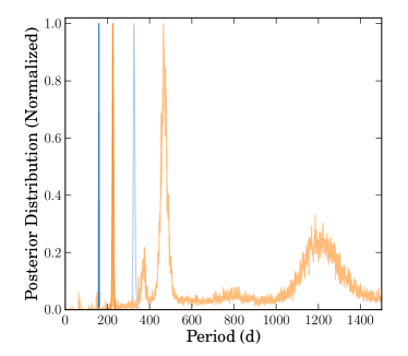
Figure 4: A comparison of the posterior probability density distributions for two periodicities in PSR J1705$-$3950 and PSR B1828$-$11, all normalized to peak amplitude. The dark and light blue lines indicate the two observed periods of PSR J1705$-$3950 and imply well-constrained detections. The short, 225-day period of PSR B1828$-$11 is likewise well-constrained (dark orange), but the addition of a second period results in many possible solutions of similar quality (light orange), including a dominant $\sim$450-day peak.

3.3 PSR B0740$-$28

Several other pulsars in our parent sample have published analyses indicating quasi-periodic profile and/or timing modulation. However, these examples seem to lack the coherence of those presented here and did not pass our selection criteria. E.g., PSR B0740$-$28 shows marked, rapid profile and spin-down variations with a time-scale of about 50 days (Lyne et al., 2010), but these oscillations are irregular. Interestingly, Keith et al. (2013) found that correlation between the spin-down properties and profile increased dramatically following a glitch, and Brook et al. (in prep.) found similar behaviour using complementary methods.

3.4 Summary

To summarise, the candidates we have identified have three key features: (1) the modulations are of high quality; (2) some show significant modulation at a harmonic, but with amplitudes about ten times smaller than the fundamental; and (3) after removing the sinusoidal modulation, the remaining the timing noise has a spectrum well described by a simple power law. The high quality factor distinguishes these objects from the “state switching” pulsars presented by Lyne et al. (2010) and Hobbs, Lyne & Kramer (2010). A further key feature of about one third of this “state switching” sample is the presence of pulse profile variation, and we proceed to search for such variation in our sample.

4 Search for Pulse Profile Variations

If the TOA modulations presented here represent a high-$\dot{E}$ continuation of the magnetospheric switching observed by Lyne et al. (2010), there we might be evidence for pulse profile variation. Unfortunately, most of our candidates are relatively radio-faint, with typical signal-to-noise ratio of 10–20 in our short (typically 2–3 minute) observations. Several pulsars also suffer strong scattering by turbulent electrons in the interstellar medium, and the multi-path propagation dilutes intrinsic profile changes.

To mitigate these limitations, we have adopted the following approach as the most sensitive to pulse profile variations correlated with TOA modulations: if the periodic behaviour is due to magnetospheric switching between $\dot{\nu}$ states, then the “zero crossing” of the residual time series indicates a switch. Timing noise complicates this prescription, and we have instead taken the best-fitting realization of the sinusoidal signals discussed above as indicative of possible state changes and co-added the profiles from the intervals with positive and negative residuals. Because the received flux density varies due to scintillation in the interstellar medium, before co-addition we normalized each profile by its measured flux density.

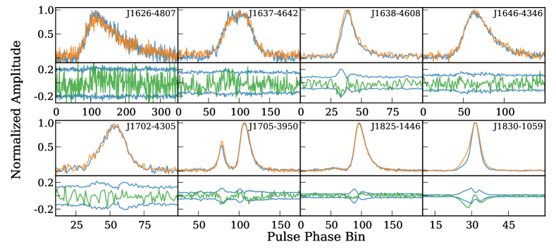
Figure 5: Analysis of profile variation. The full profiles have 512 phase bins and are zoomed to the indicated phase bins. The orange and blue traces in the upper panel show the co-added profiles obtained during periods of positive and negative timing residual, normalized by flux and aligned by TOA. The green lower panel trace shows the difference. The light blue trace shows the central 90% of differences resulting from a random shuffling of the individual profiles among groups, giving an estimate of the statistical significance of the observed differences.

The resulting co-added profiles appear in Figure 5. The lower panels show the difference between the two “states”. To determine whether any differences are statistically significant, we repeated the exercise 100 times but randomly assigned profiles to one of the two states and have plotted the envelope resulting from these simulations in the lower panel. Four pulsars are dominated by white noise and/or scattering and show no evidence of correlated profile variation: J1626$-$4807, J1637$-$4642, J1646$-$4346, and J1702$-$4306. Three pulsars, J1638$-$4608, J1705$-$3950, and J1825$-$1446, show differences significant relative to the radiometer noise level. However, the differences can be accounted for by chance, suggesting the pulse profile variation is due to jitter rather than correlated with the TOA modulation. Finally, PSR B1828$-$11 shows a clear correlation between the pulse profile state and the TOA modulation, with a narrower profile occurring when the TOA residuals are negative.

The observed profile differences in PSR B1828$-$11 are significant according to both of our tests but are substantially smaller than those observed by Stairs, Lyne & Shemar (2000). This is due to our adoption of a single sinusoid model, which as discussed above does not capture the full modulation behaviour of the pulsar. We expect it to work well for the other candidates whose modulation is dominated by the fundamental frequency.

The profile differences in J1705$-$3950, and J1825$-$1446 hint at real correlated profile changes and motivate a dedicated campaign to obtain deep observations at higher frequencies where the effects of scattering are reduced. We conclude, however, that aside from the known profile variation of PSR B1828$-$11, there is no significant profile variation in the new candidates. Brook et al. (in prep.) reach a similar conclusion using a Gaussian regression method that smoothly interpolates both profile shapes and spin-down variations between observations. This “model independent” approach avoids the need to classify observations into particular states and offers complementary verification of our results. The lack of pulse profile variation, together with the sinusoidal nature of the TOA modulation, suggests our candidates are indeed distinct from previous examples. Below, we consider mechanisms that may be responsible for the observed properties.

5 Interpretation of Periodic Signals

We have established that seven pulsars in our sample show stable, sinusoidal modulation and have no strong evidence for pulse profile variation. The regularity of these modulations requires a stable underlying clock, and the $>$100-day time-scales involved are far longer than any dynamic process expected from the neutron star magnetosphere. We thus expect the clock to be either external to the magnetosphere or associated with the neutron star itself, and we discuss a scenario for each case below. First, planetary companions naturally furnish sinusoidal modulation through reflex motion and should not perturb the pulse profile. Second, we consider the “biased magnetospheric switching” proposed by Jones (2012), in which neutron star precession drives regular magnetospheric state switching. The resulting current reconfiguration modulates the external torque, and hence the pulse TOAs, and the pulse emission profile.

5.1 Planets

Table 3: Derived parameters for periodic signals; Planetary values assume a circular orbit about a 1.4 $M_{\sun}$ neutron star. $\delta\dot{\nu}$ is computed as $(2\,a/P)(2\pi/P_{b})^{2}$.

	$P_{b}$	$m_{c}\sin i$	$a$	$\delta\dot{\nu}/\dot{\nu}$
	yr	$M_{\earth}$	AU	%
J1626$-$4807	0.76	3.03	0.95	0.68
J1637$-$4642	0.52	0.64	0.65	0.04
J1638$-$4608	1.29	6.17	1.61	0.20
	0.65	0.91	0.81
J1646$-$4346	0.33	4.54	0.41	0.38
J1702$-$4306	1.07	2.41	1.34	0.36
	0.54	0.55	0.68
J1705$-$3950	0.89	2.44	1.12	0.14
	0.43	1.01	0.55
J1825$-$1446	0.34	0.62	0.42	0.31

If interpreted as planetary companions, the TOA modulations correspond to earth-mass planets which reside within two AU of the neutron star (Table 3). As we discussed in Kerr et al. (2015), forming such massive planets within $10^{5}$ yr, the typical age of these pulsars, is challenging but not impossible, provided a disk of sufficient angular momentum is able to deposit copious dust in a relatively narrow radial range (Hansen, Shih & Currie, 2009). The radii are large enough that the effects of both tidal disruption and evaporation/heating in the pulsar wind are negligible on the growth of rocky bodies.

However, there are several arguments against a planetary interpretation. First, why have none been detected about older pulsars? Planets of these masses would be easily identifiable in such timing residuals, particularly since the level of stochastic timing noise is also reduced. Their absence in samples such as those of Hobbs, Edwards & Manchester (2006) suggests our candidates are not planets. On the other hand, planetary systems may be selected against in samples of primarily older pulsars. The orbital planes of binary systems will preferentially be more edge-on than face-on. Thus, if the neutron spin axis is aligned with the plane of its accretion/protoplanetary disk, alignment of the magnetic field with the spin axis on time-scales of $<$10⁷ yr would decrease the rate of planetary systems with visible pulsar beams. However, alignment is a slow process, if it happens at all (e.g. Tauris & Manchester, 1998), so we conclude that the lack of planet detections in other samples argues against such an interpretation for the majority of our candidates.

Secondly, at least one, and possibly three, of our candidates boast a significant harmonic modulation, implying two planets in 2:1 mean-motion resonances. Beaugé, Ferraz-Mello & Michtchenko (2003) have studied this resonance for a range of parameters, including the mass ratios $m_{2}/m_{1}>1$ we find in all of our two-sinusoid systems. The stable resonance condition requires aligned apsides and, generally, a large eccentricity for the inner (less massive) planet. The epoch of periastron measurements for the pulsars with significant second harmonics are generally not consistent with aligned apsides. Intriguingly, though, the strongest second harmonic candidate, PSR J1705$-$3950, is consistent with an aligned apsides orbit, and its implied planet masses are some of the lowest in the sample. If any of these signals correspond to planetary companions, we advance this pulsar as the most likely candidate.

On the other hand, the presence of the second harmonic could be explained with a single planet in a moderately eccentric orbit. We have performed fits of the timing modulation of PSR J1705$-$3950 and PSR J1638$-$4608 with a single, eccentric planet. While we find that the eccentricity is generally significant, the two-sinusoid models are statistically preferred, and the measured eccentricity values of 0.4 (PSR J1705$-$3950) and 0.2 (PSR J1638$-$4608) are somewhat larger than expected from oligarchical formation scenarios (Hansen, Shih & Currie, 2009).

5.2 Precession

Precession—and, specifically, free precession—coupled as it is to the large neutron star moment of inertia, makes an attractive candidate for the clock underpinning high-quality modulations. For a biaxial rotator precessing with a small “wobble angle”, the precession frequency $\nu_{p}$ is simply related to the spin frequency $\nu_{s}$ by the Eulerian relation

$$\frac{\nu_{p}}{\nu_{s}}=\frac{P_{s}}{P_{p}}=\frac{\Delta I_{p}}{I_{p}}\equiv\epsilon$$ (2)

where $\Delta I_{p}$ is the difference in moment of inertia between the symmetry axis and either of the other two axes and $I_{p}$ is the characteristic moment of inertia of the precessing body. A pedagogical derivation of this result can be found in Jones & Andersson (2001), and more complete treatments in Cutler, Ushomirsky & Link (2003), Sedrakian, Wasserman & Cordes (1999), and Wasserman (2003). A key point is that $I_{p}$ includes any parts of the neutron star tightly coupled (on time-scales $\leq P_{s}$) to the precessing crust.

Although this result is often presented in the literature, there is widespread disagreement about both $\Delta I_{p}$ and $I_{p}$, i.e. which parts of the neutron star are coupled to precessional motion, as well on damping time-scales for precession. Further complications include the rôle of external torque applied by the magnetosphere; although it generally modifies the precession dynamics only slightly, it is predominantly the time-varying external torque that produces TOA modulation. We outline these arguments and their observational implications below.

5.2.1 The Precession Frequency

For pulsars spinning at 1 Hz to precess with $\nu_{p}=1/\mathrm{yr}$, Equation 2 implies an ellipticity $\epsilon=3\times 10^{-8}$, which in turn requires the correct ratio between neutron star deformation $\Delta I_{p}$ and total moment of inertia coupled to the precession $I_{p}$.

Several mechanisms have been proposed for establishing $\Delta I_{p}$. E.g., magnetic stresses associated with the internal dipole field can provide an ellipticity of order the ratio of magnetic field energy to gravitational field energy $\epsilon\approx 10^{-12}$ (e.g. Zanazzi & Lai, 2015) with the ellipticity aligned with the magnetic moment. Together with intrinsic ellipticities, such deformations may be relevant for the claimed secular evolution of the magnetic field inclination of the Crab pulsar (Lyne et al., 2013). For large stresses, the neutron star is inherently triaxial, and interestingly, such models naturally produce relatively large modulation power in harmonics, as we observe in PSR B1828$-$11 and some members of our sample (Wasserman, 2003). Such large stresses, about two orders of magnitude above the dipole contribution, could result from a Type II superconducting core or strong toroidal fields. As we note below, though, a Type II superconducting core may inhibit low frequency precession through pinning of core neutron superfluid vortices to proton superfluid flux tubes.

A relatively natural mechanism for achieving the ellipticities required for $P_{p}=1$ yr is the strained crust. In this scenario, the crust solidifies when the neutron star is spinning rapidly, freezing in a zero strain oblateness proportional to its large spin frequency, $\epsilon_{0}\propto\nu_{0}^{2}$. As the neutron star spins down and rotational support is removed, the crustal bulge decreases, but Coulomb forces act to maintain a deformation larger than that supported by the current centrifugal force. This deformation, which depends on the ratio of the Coulomb and gravitational forces, is parameterized by the rigidity parameter $b\equiv\Delta I_{p}/\Delta I(\nu)$, with $\Delta I(\nu)$ the equatorial bulge (Jones & Andersson, 2001; Cutler, Ushomirsky & Link, 2003), and is estimated to be about $2\times 10^{-7}$ (Cutler, Ushomirsky & Link, 2003). If the crust is relaxed at the current spin rate, such a value produces ellipticity of order $3\times 10^{-11}$, while a strained crust with reference spin $\nu_{0}$ will increase the ellipticity by $(\nu_{0}/\nu_{s})^{2}$, more than two orders of magnitude if the neutron star is born spinning at tens of Hz. More precisely, Cutler, Ushomirsky & Link (2003) find

$$\frac{\Delta I_{p}}{I_{p}}\approx 9.7\times 10^{-9}\left(\frac{\nu_{0}}{40\,\mathrm{Hz}}\right)^{2}\frac{I_{p}/I_{*}}{10^{-2}}\left(\frac{M}{1.4\,M_{\sun}}\right)^{2}\left(\frac{R}{12\,\mathrm{km}}\right)^{4},$$ (3)

where as before $I_{p}$ is the moment of inertia involved in precession, and $I_{*}$ is the total moment of the neutron star. As can be seen from the strong dependence on $R$, this ellipticity can be varied by a factor of two simply by stiffening/softening the neutron star equation of state.

5.2.2 Component Coupling

A neutron star is substantially more complicated than the picture presented above. The core—containing about 90% of the moment of inertia—is thought to comprise primarily a neutron superfluid and a few per cent by mass protons (also superfluid) and electrons (degenerate). Some of the neutron superfluid is thought to penetrate the crust and its vortices pin on the crustal lattice; the spontaneous or triggered release of these pinned vortices is a plausible mechanism for the large glitches observed in young pulsars (e.g. Anderson & Itoh, 1975; Alpar & Sauls, 1988).

If some portion of superfluid is pinned to the crust, it dramatically increases the effective ellipticity (and precession frequency) as first noted by Shaham (1977). Specifically, for small wobble angles, $\nu_{p}/\nu_{s}\approx I_{pin}/I_{p}$, where the numerator is the moment of inertia of the pinned superfluid and the denominator the moment of inertia of all other precessing components. Assuming $I_{p}$ is primarily due to the crust and coupled charged protons in the core, the right-hand side of this relation is unity, ruling out long-period precession.

However, Link & Cutler (2002) have calculated that Magnus forces due to precession with modest wobble angles (3°) as proposed for PSR B1828$-$11 exceed the force keeping vortices pinned on crustal nuclei. On the other hand, precession at small wobble angles (0.1°) could allow substantial pinning. Consequently, large wobble angle precession and large amplitude glitches should be mutually exclusive phenomena, and small-amplitude precession at low frequencies may be prevented by superfluid pinning.

Equally critical is the core / crust coupling. Alpar & Sauls (1988) calculated the coupling due to the magnetisation of superfluid vortices via entrainment of protons and electrons and the subsequent scattering of charged particles. This effect couples the core to the crust on time-scales of 400–10,000 P_s. This coupling is weak in terms of precession, and the core moment of inertia is effectively decoupled from the precession. The coupling will weakly damp precession on time-scales of 400–10,000 P_p (Sedrakian, Wasserman & Cordes, 1999). Although we will not discuss it here, we note that instabilities arising from the velocity differential between the two superfluids may complicate this picture (Glampedakis, Andersson & Jones, 2009).

Link (2003) notes that interaction between neutron superfluid vortices and magnetic flux tubes in the proton superfluid in the core (see also Chau, Cheng & Ding, 1992) can either (1) lock the core to the crust (short coupling time) or (2) dissipate precessional motion on time-scales of hours via kelvon excitation. He concludes $P_{p}=$1 yr precession implies that the core proton superfluid is a Type 1 superconductor, effectively separating vortices and flux tubes. However, the details of these calculations depend sensitively on the poorly known distribution of the constituents of the core, e.g. strong toroidal fields (e.g. Sidery & Alpar, 2009). Indeed, Haskell, Pizzochero & Seveso (2013) argue that such pinning would also prohibit the large glitches observed in PSR J0835$-$4510 (Vela).

5.2.3 External Torques

Until now, we have neglected external torques in our discussion. However, they are important in establishing the observational implications of precession. Generally, these torques trivially modify the precessional motion of interest, but the spin-down rate of the neutron star depends on the magnetic inclination $\alpha$, and precession gives $\alpha$ dependency on time. Indeed, even in the absence of precession, external torques tend to force $\alpha\rightarrow 0$, but only on the pulsar spin-down time-scale (Melatos, 2000). Most calculations of, e.g., the time-dependent spin-down rate under precessional motion are in the vacuum limit (Link & Epstein, 2001; Jones & Andersson, 2001; Wasserman, 2003). Their application to PSR B1828$-$11 results in extremely stringent constraints on the magnetic inclination, viz. that it be orthogonal to the spin axis to within 1°, a prediction at odds with the lack of an observed interpulse from the opposite magnetic pole. More recent calculations make use of numerical modelling of force-free magnetospheres, with substantially altered torques on the neutron star surface (Arzamasskiy, Philippov & Tchekhovskoy, 2015) that allow for broader range of $\alpha$ in describing PSR B1828$-$11. Interestingly, dominant magnetic stresses allow an even larger range of $\alpha$ (Wasserman, 2003; Akgün, Link & Wasserman, 2006).

5.2.4 Observations

Despite the large body of work on neutron star precession, whose surface we have only scratched here, the verdict still seems to be out on whether or not (1) it can proceed at all; (2) it can operate on annual time-scales; (3) it can persist as a high-quality-factor signature in pulse times of arrival. We therefore proceed in an empirical fashion and study the implications of the observed modulations for a precession interpretation.

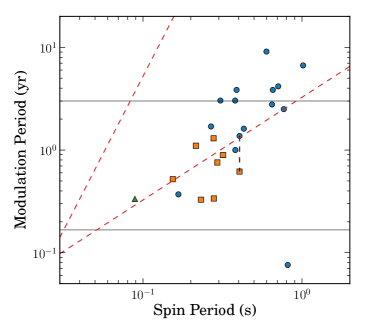
Figure 6: The observed modulation period for our sample (orange squares) and the 15 pulsars from the Lyne et al. (2010) sample as characterised by Jones (2012, blue circles). The green triangle shows the 122 d period inferred by Durant et al. (2013) from the helical jet of PSR J0835$-$4510. The solid, horizontal lines indicate, approximately, the range of modulation periods to which our analysis is sensitive. The dashed lines represent the expected modulation period for 1.4 $M_{\sun}$, 12 km neutron stars with a frozen in strain corresponding to a reference spin of 40 Hz (see Equation 3; linear dependence on spin period and shorter modulation periods) and those for similar neutron stars with relaxed crusts ($\propto P_{s}^{3}$, and longer modulation period). We have shown PSR B1828$-$11 with our measured period (225 days) as well as that calculated by Jones (2012), about twice as long. The outlier with modulation period $<$0.1 yr is PSR B1931$+$24.

In Figure 6, we have plotted the measured modulation periods from our sample (orange) along with the values measured by Jones (2012) from the sample of Lyne et al. (2010) as a function of pulsar spin period. If the modulation is due to precession of a neutron star with a strained crust, $P_{p}\propto P_{s}$, and a reference spin of 40 Hz yields a strain level that reproduces the observed modulation period within an order of magnitude. However, the observed dependence is somewhat steeper, with a best-fit relation $P_{m}/\mathrm{yr}=7.1\,P_{s}^{1.5}$. On the other hand, if the neutron star crusts are fully relaxed at the current spin period, $P_{p}\propto P_{s}^{3}$ and, due to the reduced ellipticity, predictions for $P_{p}$ are much longer. Finally, we note that some of the period measurements from Jones (2012) may be biased to larger values: these oscillations are of lower quality factor and some cycles may be “missing”, in which case the measurement procedure gives a result longer than the true modulation period. Correcting this bias would alleviate some of the tension with the strained crust picture.

The obvious outlier in Figure 6 is the intermittent pulsar PSR B1931$+$24 (Kramer et al., 2006), which we have included for comparison. None of the mechanisms described above are plausible if its intermittency is interpreted as precession.

We have also included the recent detection of helical motion in the X-ray jet of Vela (Durant et al., 2013) with an apparent period of 122 d, although shorter periods (as aliases) are allowed. If the corkscrew motion is due to pulsar precession, the measured value is in general agreement with the observed trend.

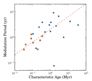
Figure 7: As Figure 6 but with characteristic age as abscissa. The dashed line gives the prediction of Equation 4.

Next, we consider a scenario in which magnetic stresses dominate the ellipticity. Dipole stresses are generally too small to provide the observed periods, but for completeness we note they predict $P_{p}\propto 1/\dot{P_{s}}$, i.e. no dependence on $P_{s}$, in poor agreement with the observations. For a superconducting core (Wasserman, 2003), Jones (2012) gives the relation as

$$\frac{P_{p}}{1\,\mathrm{yr}}=2.0\left(\frac{\tau_{sd}}{10^{6}\,\mathrm{yr}}\right)^{1/2}\left(\frac{2\times 10^{15}\,\mathrm{G}}{H_{c}}\right)\left(\frac{I_{p}}{I_{*}}\right)$$ (4)

with $\tau_{sd}\equiv P_{s}/2\dot{P_{s}}$ the characteristic pulsar age and $H_{c}$ the critical field due to the superconducting core. Accordingly, we have plotted the modulation periods against characteristic age in Figure 7 along with the trend of Equation 4. The relation describes both the magnitude and trend of the data reasonably well. But, we note that the predicted modulation periods require the entire neutron star to participate in precession ($I_{p}=I_{*}$). If, instead, only the crust participates ($I_{p}\approx 0.01I_{*}$), the precession periods are too rapid to fit the observations.

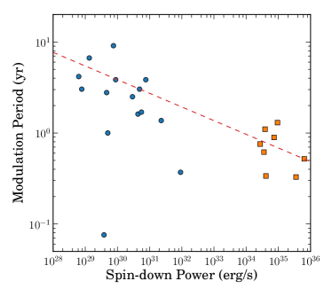
Figure 8: As Figure 6 but with spin-down power as abscissa. The line is simply to guide the eye and is $\propto\dot{E}^{-0.15}.$

In Figure 8, we show the dependence of the observed modulation period on spin-down power ($\dot{E}\propto\dot{P_{s}}/P_{s}^{3}$). The scatter is relatively narrow, in keeping with our finding that the data depend maximally on $P_{s}$ and little on $\dot{P_{s}}$, i.e. $P_{m}/\mathrm{yr}=8.6\,P_{s}^{1.35}\dot{P_{s}}^{-0.15}$. We also see an interesting gap in parameter space coverage, motivating a timing program targetting pulsars in the range $10^{31}<\dot{E}/\mathrm{erg\,s^{-1}}<10^{34}$.

We conclude this section by briefly considering millisecond pulsars (MSPs). The timing precision can easily reach $<$1 $\mu$s, particularly for pulsars monitored by timing arrays (e.g. Manchester et al., 2013). Despite this sensitivity, no similar harmonic oscillations have been observed. This result is not surprising, however, if any of the precession mechanisms proposed above are in play. During the spin-up process, neuton star crusts are likely to break under the substantial centrifugal force and distribution of accreted material, so the crusts of current MSPs are likely to be relaxed, and Equation 3 indicates ellipticies of about $10^{-6}$ in this case, with precession periods of about an hour. In the case of magnetic stresses, the much weaker dipole magnetic fields would push the precession period higher, even when allowing for a superconducting core. Equation 4 with a typical MSP age $\tau_{sd}=10^{9}$ yr suggests a precession period of about 60 years, though for crust-only precession this drops to 1–2 years. All cases would require some continual mechanism to excite the precession in order for it to be observable.

6 Discussion

As we have discussed above, we cannot rule out planets as the source of the nearly sinusoidal TOA modulations we observe and perhaps one of our systems harbours bona fide planets. Our preferred clock, however, is neutron star precession, but the extent to which it can operate in real neutron stars is unclear. Regardless of the actual mechanism, we can ask: is the same mechanism responsible for both the longer period, lower quality oscillations of Lyne et al. (2010) and the shorter period, higher quality modulations of our sample? To address this, we amplify on the idea of Jones (2012), viz. that a pulsar may lie on the cusp of two different magnetospheric configurations, and that the precessional phase alters the probability that the pulsar may switch between them. Cordes (2013) has analyzed a similar scenario with forced Markov processes to model state-changing pulsars. In both situations, the altered magnetosphere acts as a “lever arm” to enhance the observational signature of potentially minor underlying changes.

Can such a mechanism unify the two samples? We present a qualitative argument that it can. The most dramatic changes in spin-down rate, of order unity, are associated with intermittent pulsars (Kramer et al., 2006; Camilo et al., 2012; Lorimer et al., 2012). The magnetospheric currents are clearly dramatically reconfigured during the state change that turns the pulsar off. Large changes in the plasma density of the magnetosphere of PSR B0943$+$10 (Hermsen et al., 2013) happen rapidly when the pulsar changes between its radio-bright and radio-faint states. These pulsars tend to be at least 1 Myr old, suggesting that the stable states of old pulsar magnetospheres are separated by large energy barriers. In contrast, the modulated pulsars of Lyne et al. (2010) show much more modest changes in $\dot{\nu}$, typically 1%, and the pulse profile variations can be quite subtle. For our sample, the fractional $\dot{\nu}$ changes are even smaller (Table 3), all well less than 1%, and as discussed in §4, there is no evidence for profile variation.

Thus, we posit that pulsars have one or more metastable magnetospheric states whose properties change with age. For young pulsars, these states are finely separated in activation energy, and may even form a continuum. As the pulsar ages, its magnetosphere evolves discrete states more widely discrepant in currents, beam patterns, and spin-down torques; in some states the current configurations may limit particle acceleration processes. Thus, in young pulsars, very small amplitude (wobble angle) precession could smoothly modulate the current structure in the magnetosphere, with the latter enhancing the change in spin-down rate from that expected simply from changing the magnetic inclination (c.f. Arzamasskiy, Philippov & Tchekhovskoy, 2015). With increasing age, the transition between states becomes more stochastic, the higher activation energy preventing the magnetosphere from smoothly following the precession. The quality factor of the modulations drops, and profile variation becomes evident, e.g. as in the $\sim$600 d cycle of PSR B0916$+$06 (Perera et al., 2015). In some cycles, a state change may not occur at all, perhaps explaining “missing” $\dot{\nu}$ cycles like those visible in the time series of PSR B1642$-$03 (Lyne et al., 2010). Extreme versions of this situation may account for “episodic” events like the profile change of PSR J0738$-$4042 (Brook et al., 2014), attributed by those authors to an encounter with an asteroid. For that event, we argue that the continued profile changes after the sudden shift may be more easily attribute to an ongoing process like precession. Eventually, the precession is no longer able to drive the star into different states, and whatever pulse modulation effects occur through modulation of $\alpha$ are too small to observe. Precessionaly motion itself may likewise be difficult to maintain in older pulsars if glitches or timing noise are responsible for its excitation.

Indeed, glitches add two final complicating anecdotes. First, the change in correlation between spin-down and profile variation observed by Keith, Shannon & Johnston (2013) for PSR B0740$-$28 suggests that relatively minor variations in the neutron star rotation can indeed effect magnetospheric changes, in support of our scenario above. Second, the TOA modulation we observed in PSR J1646$-$4346 appears to be consistent through a large glitch ($\delta\nu=3.7\times 10^{-5}$ Hz, $\delta\nu/\nu=8.5\times 10^{-6}$, $\delta\dot{\nu}/\dot{\nu}=0.61$%). The substantial amplitude implies a large amount of the core superfluid was pinned prior to the glitch, necessitating small wobble angles to preserve the pinning. Such substantial superfluid pinning would tend to raise the precession frequency dramatically.

7 Summary and Conclusion

We have detected nearly-sinusoidal TOA modulation in seven members of a population of 151 energetic pulsars. Other candidates may lurk below our sensitivity limit, indicating such modulation is a relatively common phenomenon. This prevalence, together with the regularity of the modulation, seems to demand a dynamic process rooted in the neutron star, and we suggest precession may provide the “clock”. Observational and theoretical difficulties with modest wobble angles can be resolved by letting very small wobbles drive magnetospheric state switches. Due to the strength of the harmonics in the the TOA modulations, as well as the expectation that the core should couple tightly to the crust, we propose magnetic stresses supported by the superconducting core as the most likely source of the ellipticity required for precession.

References

- Akgün, Link & Wasserman (2006) Akgün T., Link B., Wasserman I., 2006, MNRAS, 365, 653
- Alpar & Sauls (1988) Alpar M. A., Sauls J. A., 1988, ApJ, 327, 723
- Anderson & Itoh (1975) Anderson P. W., Itoh N., 1975, Nature, 256, 25
- Arzamasskiy, Philippov & Tchekhovskoy (2015) Arzamasskiy L., Philippov A., Tchekhovskoy A., 2015, ArXiv e-prints
- Beaugé, Ferraz-Mello & Michtchenko (2003) Beaugé C., Ferraz-Mello S., Michtchenko T. A., 2003, ApJ, 593, 1124
- Brook et al. (in prep.) Brook P., Karasterigiou A., Johnston S., Kerr M., Shannon R. M., in prep., ApJ
- Brook et al. (2014) Brook P. R., Karastergiou A., Buchner S., Roberts S. J., Keith M. J., Johnston S., Shannon R. M., 2014, ApJ, 780, L31
- Camilo et al. (2012) Camilo F., Ransom S. M., Chatterjee S., Johnston S., Demorest P., 2012, ApJ, 746, 63
- Chau, Cheng & Ding (1992) Chau H. F., Cheng K. S., Ding K. Y., 1992, ApJ, 399, 213
- Coles et al. (2011) Coles W., Hobbs G., Champion D. J., Manchester R. N., Verbiest J. P. W., 2011, MNRAS, 418, 561
- Cordes (2013) Cordes J. M., 2013, ApJ, 775, 47
- Cutler, Ushomirsky & Link (2003) Cutler C., Ushomirsky G., Link B., 2003, ApJ, 588, 975
- Durant et al. (2013) Durant M., Kargaltsev O., Pavlov G. G., Kropotina J., Levenfish K., 2013, ApJ, 763, 72
- Foreman-Mackey et al. (2013) Foreman-Mackey D., Hogg D. W., Lang D., Goodman J., 2013, PASP, 125, 306
- Glampedakis, Andersson & Jones (2009) Glampedakis K., Andersson N., Jones D. I., 2009, MNRAS, 394, 1908
- Hansen, Shih & Currie (2009) Hansen B. M. S., Shih H.-Y., Currie T., 2009, ApJ, 691, 382
- Haskell, Pizzochero & Seveso (2013) Haskell B., Pizzochero P. M., Seveso S., 2013, ApJ, 764, L25
- Hermsen et al. (2013) Hermsen W. et al., 2013, Science, 339, 436
- Hewish et al. (1968) Hewish A., Bell S. J., Pilkington J. D. H., Scott P. F., Collins R. A., 1968, Nature, 217, 709
- Hobbs et al. (2010) Hobbs G. et al., 2010, Classical and Quantum Gravity, 27, 084013
- Hobbs, Lyne & Kramer (2010) Hobbs G., Lyne A. G., Kramer M., 2010, MNRAS, 402, 1027
- Hobbs, Edwards & Manchester (2006) Hobbs G. B., Edwards R. T., Manchester R. N., 2006, MNRAS, 369, 655
- Hulse & Taylor (1975) Hulse R. A., Taylor J. H., 1975, ApJ, 195, L51
- Jones (2012) Jones D. I., 2012, MNRAS, 420, 2325
- Jones & Andersson (2001) Jones D. I., Andersson N., 2001, MNRAS, 324, 811
- Keith et al. (2013) Keith M. J. et al., 2013, MNRAS, 429, 2161
- Keith, Shannon & Johnston (2013) Keith M. J., Shannon R. M., Johnston S., 2013, MNRAS, 432, 3080
- Kerr (2015) Kerr M., 2015, MNRAS, 452, 607
- Kerr et al. (2015) Kerr M., Johnston S., Hobbs G., Shannon R. M., 2015, ApJ, 809, L11
- Kramer et al. (2006) Kramer M., Lyne A. G., O’Brien J. T., Jordan C. A., Lorimer D. R., 2006, Science, 312, 549
- Link (2003) Link B., 2003, Physical Review Letters, 91, 101101
- Link & Cutler (2002) Link B., Cutler C., 2002, MNRAS, 336, 211
- Link & Epstein (2001) Link B., Epstein R. I., 2001, ApJ, 556, 392
- Lorimer et al. (2012) Lorimer D. R., Lyne A. G., McLaughlin M. A., Kramer M., Pavlov G. G., Chang C., 2012, ApJ, 758, 141
- Lyne et al. (2013) Lyne A., Graham-Smith F., Weltevrede P., Jordan C., Stappers B., Bassa C., Kramer M., 2013, Science, 342, 598
- Lyne et al. (2010) Lyne A., Hobbs G., Kramer M., Stairs I., Stappers B., 2010, Science, 329, 408
- Manchester et al. (2013) Manchester R. N. et al., 2013, Publ. Astron. Soc. Australia, 30, 17
- Melatos (2000) Melatos A., 2000, MNRAS, 313, 217
- Perera et al. (2015) Perera B. B. P., Stappers B. W., Weltevrede P., Lyne A. G., Bassa C. G., 2015, MNRAS, 446, 1380
- Sedrakian, Wasserman & Cordes (1999) Sedrakian A., Wasserman I., Cordes J. M., 1999, ApJ, 524, 341
- Shaham (1977) Shaham J., 1977, ApJ, 214, 251
- Shannon et al. (2014) Shannon R. M. et al., 2014, MNRAS, 443, 1463
- Sidery & Alpar (2009) Sidery T., Alpar M. A., 2009, MNRAS, 400, 1859
- Stairs, Lyne & Shemar (2000) Stairs I. H., Lyne A. G., Shemar S. L., 2000, Nature, 406, 484
- Tauris & Manchester (1998) Tauris T. M., Manchester R. N., 1998, MNRAS, 298, 625
- Wasserman (2003) Wasserman I., 2003, MNRAS, 341, 1020
- Wolszczan & Frail (1992) Wolszczan A., Frail D. A., 1992, Nature, 355, 145
- Zanazzi & Lai (2015) Zanazzi J. J., Lai D., 2015, MNRAS, 451, 695