Hypergraph-Based Analysis of Clustered Cooperative Beamforming with Application to Edge Caching

Abstract

The evaluation of the performance of clustered cooperative beamforming in cellular networks generally requires the solution of complex non-convex optimization problems. In this letter, a framework based on a hypergraph formalism is proposed that enables the derivation of a performance characterization of clustered cooperative beamforming in terms of per-user degrees of freedom (DoF) via the efficient solution of a coloring problem. An emerging scenario in which clusters of cooperative base stations (BSs) arise is given by cellular networks with edge caching. In fact, clusters of BSs that share the same requested files can jointly beamform the corresponding encoded signals. Based on this observation, the proposed framework is applied to obtain quantitative insights into the optimal use of cache and backhaul resources in cellular systems with edge caching. Numerical examples are provided to illustrate the merits of the proposed framework.

I Introduction

A key technology that has been recently introduced in the operation of wireless cellular systems is cooperative beamforming across non co-located base stations (BSs). Cooperative beamforming is typically enabled either by the transmission on backhaul links of common data streams to a cluster of BSs, or by joint baseband processing carried out at “cloud” processor on behalf of the cluster of BSs [1]. Recently, a new technology has emerged that enables cooperative beamforming across a cluster of BSs that share the same content by exploiting the BSs’ local storage, namely edge caching [2].

The key idea of edge caching is that of pre-fetching the most requested files based on their popularity ranking with the goal of decreasing the number of accesses to the content provider through the backhaul [3]. In this framework, cooperative beamforming is enabled by storing identical files at nearby BSs [2, 4, 5, 6, 7].

An example of a network that enables clustered cooperative beamforming is shown in Fig. 1. As seen, each content $f_{k}$ requested by each mobile station (MS) is available at a cluster of BSs, which can perform cooperative beamforming on the resulting encoded signal. For instance, content $f_{1}$ is available at the cluster of BSs $\{\text{BS}_{1},\text{BS}_{2},\text{BS}_{3}\}$ (A full description of this model in the context of cache-based networks can be found in Sec. IV). The performance analysis of a system with a general cluster assignment, including possibly overlapping clusters, such as in Fig. 1, typically requires solving complex optimization problems (see [8] and references therein).

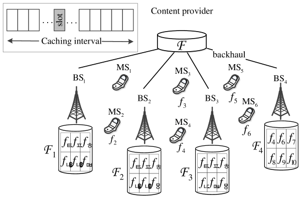
Figure 1: Illustration of a system with clustered cooperative beamforming enabled by edge caching, with indication of the set of files $\mathcal{F}_{m}$ available at each BS $m$.

In contrast, quantitative performance assessment can be carried out for a number of special message assignments using the high signal-to-noise ratio (SNR) metric of degrees of freedom (DoF) [7]. Nevertheless, to the best of the authors’ knowledge, there is no general approach to analyze arbitrary message assignments. This letter proposes a simple framework that aims at accomplishing this goal for a densely deployed wireless network. The approach is based on a hypergraph formalism and focuses on the performance of a scheme that uses zero-forcing beamforming and the orthogonal scheduling of distinct BSs’ clusters.

Based on the discussion above, the proposed method can be used to obtain quantitative insights into the optimal use of backhaul and caching resources in cache-based wireless networks using the DoF as performance metric. As a further reference to prior work, we observe that the joint design of beamforming and backhaul allocation, where the latter determines which BSs receive each non-cached file on the backhaul, is studied in [5] for a fixed pre-defined cache allocation. In [6], instead, the cache allocation problem is studied from the point of view of DoF under the assumption that all the requested files are cached at BSs.

The rest of the letter is organized as follows. Sec. II presents the system model and Sec. III the proposed hypergraph-based approach. Sec. IV discuss the application to edge caching and Sec. V provides some numerical results.

II Clustered Beamforming Model

In this section, we describe the system model for clustered cooperative beamforming. We consider a wireless network that includes a set ${\cal M}$ of $M$ BSs and a set ${\cal K}$ of $K$ mobile stations (MSs). BSs and MSs have a single antenna and spatial multiplexing is enabled only by BSs’ cooperation. The extension to case of multiple antennas is feasible with minor modification but is not covered here. The network is assumed to be dense in the sense that each MS is in the coverage area of all BSs, i.e., the channel gain from each BS to any MS is non-zero or, equivalently, the network is fully connected. The power of each BS is denoted as $P$. Moreover, we assume no time or frequency diversity so that inteference alignment based on symbol extentions is not allowed [7].

Each MS $k$ requests a message, or file, $f_{k}$. Each BS $m$ has available a subset of the requested messages, which we denote as $\mathcal{F}_{m}$ as shown in Fig. 1. All the BSs that have the same message can perform cooperative beamforming for transmission of the corresponding encoded signal. Note that this assumes the standard conditions of synchronization and channel state information availability that are pre-requisites for cooperative beamforming (see, e.g., [1]). We define the set $\mathcal{F}_{\mathrm{r}}=\{f_{k}\in\mathcal{F}:\textrm{ }k=1,..,K\}$ that includes the $K$ messages that are requested by all $K$ MSs.

Finally, we assume that the MSs are to be served with an equal rate $R(P)$ [bit/s/Hz], hence guaranteeing fairness, where we explicitly denote the dependence on the transmitted power $P$.

III DoF Analysis of Clustered Beamforming

In this section, we propose an hypergraph-based framework to evaluate a high-SNR characterization of an achievable equal rate $R(P)$. We recall that, if each MS is served at a spectral efficiency $R(P)$ then the corresponding number of DoF per user that are achievable with the given transmission scheme is defined as [7]

$$\text{per-MS DoF}=\underset{P\rightarrow\infty}{\text{lim}}\frac{R(P)}{\text{log}_{2}P}.$$ (1)

III-A Cooperative Beamforming Scheme

In order to obtain an achievable DoF metric for arbitrary MSs’ requests and sets $\mathcal{F}_{m},m=1,...,M$, we consider a natural scheme in which clusters of cooperative BSs, not necessarily disjoint, are scheduled in orthogonal spectral resources. We adopt such a scheme for its practicality and simplicity. While an enhanced performance (1) may be generally obtained by means of complex techniques such as real interference aligment [7], we contend the considered scheme appears to be strongly justified as any inter-cluster interference would in practice negatively affect the DoF metric.

To select the cooperative clusters, we note that, if all BSs in a cluster have all the files requested by an equal number of MSs, then all the MSs in this subset can be served with no mutual interference by means of zero-forcing beamforming. This holds under the mentioned assumption that the network is dense and hence each MS may be served with non-negligible receiving power by any BS of the set. We define a subset of MSs as an independent set if a subset of BSs of equal cardinality exists in which all BSs have all the messages requested by the given set of MSs. MSs in an independent sets can be served with no mutual interference via zero-forcing beamforming. We emphasize that, although the clusters of cooperative BSs are not necessarily disjoint, the independent sets of MSs are non-intersecting. For example, in Fig. 1, the subset {$\text{MS}_{1},\text{MS}_{2},\text{MS}_{3}$} is an independent set because the BSs {$\text{BS}_{1},\text{BS}_{2},\text{BS}_{3}$} all have the files {$f_{1},f_{2},f_{3}$} which are requested by the MSs in this subset.

The scheme at hand then works as follows. In each slot, the MSs are partitioned into disjoint independent sets, and all independent sets, along with their corresponding clusters of BSs, are scheduled on orthogonal time-frequency resources. Therefore, dividing the available time-frequency resources equally among all the independent sets, a DoF equal to $1/\mathcal{X}$, where $\mathcal{X}$ is the number of independent sets, can be achieved on the downlink channel. In the example of Fig. 1, beside the independent set {$\text{MS}_{1},\text{MS}_{2},\text{MS}_{3}$}, the remaining three MSs cannot be served simultaneously by any subsets of four BSs. Instead, any two of these MSs can be served by at least two BSs to form an independent set. Hence, we can take $\left\{\left\{\text{MS}_{1},\text{MS}_{2},\text{MS}_{3}\right\},\left\{\text{MS}_{4},\text{MS}_{5}\right\},\left\{\text{MS}_{6}\right\}\right\}$ as subsets defining the desired partition. The resulting per-MS DoF on the downlink is hence 1/3.

As a summary, the per-MS DoF achieved by the scheme at hand is given as

$$\text{per-MS DoF}=\frac{1}{\mathcal{X}},$$ (2)

where $\mathcal{X}$ is the number of independent sets of MSs. The rest of this section is devoted to the calculation of the minimum number of independent sets $\mathcal{X}$ through a hypergraph coloring problem.

III-B Hypergraph Framework

A hypergraph $\mathcal{H}=(\mathcal{K},\mathcal{E})$, where the vertex set $\mathcal{K}$ is the set of MSs and $\mathcal{E}$ is the set of hyperedges associated to a given allocation of files across the BSs and to a set of MSs’ requests. A hyperedge $e\subseteq\mathcal{K}$ is in $\mathcal{E}$ if there is no subset of $\left|e\right|$ BSs such that each BS in the subset has all the files requested by the MSs in the set $e$. Under this definition, the independent sets introduced above correspond exactly to the independent sets of $\mathcal{H}$. We recall in fact that an independent set of a hypergraph $\mathcal{H}$ is a subset of the vertex set such that no subset of this set is a hyperedge of $\mathcal{H}$ [9].

We focus with no loss of generality of simple hypergraphs in which only minimal hyperedges are included in $\mathcal{E}$ [9]. A hyperedge $e\in\mathcal{E}$ is minimal if no subsets of $e^{\prime}\subseteq e$ is an hyperedge. In our context, this implies that, if a hyperedge of cardinality $\left|e\right|$ exists, then all subsets of $e$ with cardinality less than $\left|e\right|$ correspond to independent sets and hence zero-forcing joint beamforming is possible within any such subset. In Fig. 2a shows the hypergraph associated to the network configuration in Fig. 1 considering only the files in the BSs’ caches.

The minimum number of independent sets of $\mathcal{H}$ is known as the chromatic number $\mathcal{X}$ and corresponds exactly to the number of independent sets of MSs introduced above. Calculating the chromatic number $\mathcal{X}$ requires solving the hypergraph coloring problem, which is known to be NP-hard [9]. The hypergraph coloring problem consists of the assignment to each vertex of a hypergraph $\mathcal{H}$ a color of such no hyperedge is monochromatic. Here we resort to a standard greedy coloring algorithm as detailed in, e.g., [9]. The hypergraph coloring problem consists of the assignment of a color to each vertex of a hypergraph $\mathcal{H}$, such that no hyperedge is monochromatic. Note that colors are identified by integer numbers and that $\mathcal{X}$ equals to the maximum number used to color the vertices of hypergraph. Once coloring is completed, subsets of vertices with the same color form disjoint independent sets and hence should be scheduled in different spectral resources. An example is shown in Fig. 2b in which we fix the permutation $i_{1},i_{2},\ldots,i_{\mathcal{K}}$ as $\text{MS}_{1},\text{MS}_{2},\text{MS}_{3},\text{MS}_{4},\text{MS}_{5},\text{MS}_{6}$ and apply the greedy coloring algorithm in [9].

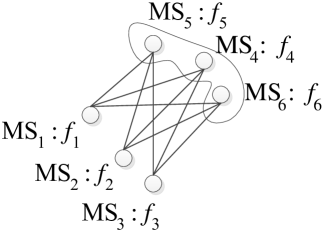
(a)

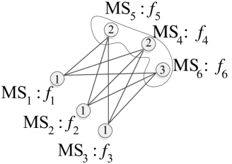
(b)

Figure 2: (a) Illustration of hypergraph $\mathcal{H}$ associated with the configuration in Fig. 1. Hyperedges of cardinality 2 are represented as regular edges, while the hyperedges of larger cardinality are represented as closed curves including a set of vertices. (b) Illustration of a colored hypergraph, solved with a standard greedy coloring, associated to the MSs in Fig. 1, where numbers on the vertices indicate colors.

IV Application to Edge Caching

The framework described above can be applied to obtain quantitative insights into optimal use of cache and backhaul resources. This application is discussed in this section.

IV-A Edge Caching Model

In a cache-based wireless network, each BS $m$ is endowed with a cache that can store a set of $N$ files and is connected to the content provider via a backhaul link that can deliver up to $\mathcal{C}\text{log}P$ bit/s/Hz, where $\mathcal{C}$ is the backhaul capacity measured in terms of DoF. The files are selected from a set $\mathcal{F}$ of popular files that remains constant for a period referred to as caching interval. We label the files in decreasing order of popularity in a given caching interval, so that the file set is indicated as $\mathcal{F}=\{1,2,\ldots,F\}$, where $f\in F$ is the $f$th most popular file. We define as $\mathcal{F}_{\text{c},m}$ the set of files cached by BS $m$ for a given caching interval.

Time is characterized by two different scales so that each caching interval contains multiple slots, as shown in the inset of Fig. 1. At any slot, each MS $k$ requests a file $f_{k}\in\mathcal{F}$ independently of the others according to the classical Zipf popularity distribution with parameter $\gamma\geq 0$, i.e., with probability $P_{f}=f^{-\gamma}\diagup\sum_{f=1}^{F}f^{-\gamma}$. For any given slot, we define the set $\mathcal{F}_{\mathrm{r}}=\{f_{k}\in\mathcal{F}:\textrm{ }k=1,..,K\}$ that includes the $K$ files that are requested by all MSs. Note that any file in the set $\mathcal{F}_{\mathrm{r}}\backslash\mathcal{F}_{\mathrm{c}}=\cup_{m=1}^{M}\mathcal{F}_{\text{c},m}$, if requested, needs to be downloaded on the backhaul links of some BSs in order to be transmitted to the requesting MSs. We also observe that the equal rate $R(P)$ at which transmission is possible in a slot, generally changes from slot to slot due to the varying MSs’ requests.

IV-B DoF Analysis of Caching and Backhaul Policies

The design of the edge caching system requires the definition of the policies used to populate the caches and to allocate the backhaul resources. The caching allocation policy, which is to be applied at the long time-scale of caching intervals, determines the subset $\mathcal{F}_{\text{c},m}$ of files that each BS $m$ in the network caches for a caching interval. Instead, the backhaul allocation policy is applied in each slot to determine which files in the set $\mathcal{F}_{\mathrm{r}}\backslash\mathcal{F}_{\mathrm{c}}$ of files that are requested but not in the caches should be sent on each backhaul link to the connected BS. We next provide some examples of basic caching and backhaul policies that will be considered in the numerical results of Sec. V.

Examples of caching policies

(i) Cache Most Popular (CMP): All the BSs pre-fetch the $N$ most popular files for caching. Note that CMP enables full cooperation among the BSs on the transmission of the cached files but may cause a significant number of cache misses if $N$ is small. (ii) Cache Distinct (CD): For a given arbitrary order of the BSs, the first BS stores the $N$ most popular files, the second BS the next $N$ most popular files, and so on, in such a way that, assuming that $MN\leq F$, there is no duplication of files in the BSs’ caches. CD makes joint beamforming impossible, at least based solely on the cached files, but it minimizes the probability of a cache miss. (iii) Hybrid Caching (HC): All BSs cache the same $N_{\text{CMP}}\leq N$ most popular files to induce cooperative transmission, and then different BSs cache distinct files from the rest of the files following the CD policy. Note that HC generalizes both CMP and CD.

Example of backhaul policy

Due to space constraint, we mention here on the simple Greedy Download (GD) policy. This policy allocates each missing file in $\mathcal{F}_{\mathrm{r}}\backslash\mathcal{F}_{\mathrm{c}}$, following some pre-specified order (here, the order of popularity), to a subset of BSs that yields the largest per-MS DoF detailed below.

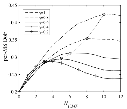
Figure 3: Per-MS DoF of the HC caching policy under GD backhaul policy for different popularity distribution exponents $\gamma$ ($N=12,M=K=5,F=60$).

For any given caching and backhaul policy, at any slot, the model reduces to the one studied in the previous sections in which each MS requests a file and each BS $m$ has available a subset $\mathcal{F}_{m}$ of the files. Note that the set $\mathcal{F}_{m}$ contains both the files in $\mathcal{F}_{\text{c},m}$ that are present in the cache of BS $m$ and also the files that have been downloaded on the corresponding backhaul link. Therefore, we can adopt the framework developed in Sec. III in order to obtain an assessment of the per-MS DoF in any given slot. To this end, denote as $F_{max}$ the maximum number of files transmitted on a backhaul link to any BS by the given backhaul transmission policy. The per-DoF is then limited, not only by the downlink DoF studied in Sec. III, but also by $\mathcal{C}/F_{max}$. This is because the equal rate $R(P)$ cannot be larger than the rate supported on the backhaul link if at least one of the files needs to be downloaded from the content provider. The per-MS DoF achieved in a given slot is then evaluated as

$$\text{per-MS DoF}=\text{min}\left(\frac{\mathcal{C}}{F_{max}},\frac{1}{\mathcal{X}}\right),$$ (3)

where $\mathcal{X}$ is the chromatic number of the hypergraph corresponding to the configuration of MSs’ requests and caches in the given slot. The performance of specified caching and backhaul policies can then be assessed by averaging (3) over the randomness of the MSs’ requests.

V Numerical Results

In this section, we provide some numerical example in order to illustrate the type of conclusions that can be obtained by means of the proposed framework. We emphasize again that the results can be obtained in a straightforward manner by implementing the hypergraph coloring approach discussed in Sec. III. We focus on edge caching and show in Fig. 3 the average per-MS DoF, obtained from (3), for the HC caching policy and GD backhaul policy versus the number of files $N_{\text{CMP}}$ to be stored at all caches. Different curves are obtained by varying the popularity exponent $\gamma$. For a larger $\gamma$, allocating a bigger part of the cache to the same files, as measured by $N_{\text{CMP}}$, yields a higher per-MS DoF, as this maximize the cooperation opportunities without causing too many cache misses. In particular, Fig. 3 enables the quantitative estimate of the optimal value of $N_{\text{CMP}}$, as indicated by the dotted line.

To get more insight into the comparison between the CMP ($N_{\text{CMP}}=N$) and CD ($N_{\text{CMP}}=0$) caching policies, Fig. 4 represents the regions of backhaul DoF $\mathcal{C}$ and cache size $N$ values in which the CMP or CD caching policy outperforms the other under the GD backhaul policy as a function of the popularity exponent $\gamma$. The figure allows to obtain the values of $N$ above which CMP is advantageous for a fixed $\mathcal{C}$, or, for a fixed $N$, the values of $\mathcal{C}$ that are sufficiently large to compensate for the cache miss events.

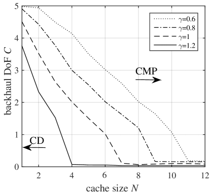
Figure 4: Regions of backhaul DoF $\mathcal{C}$ and cache size $N$ values in which CMP (right of the curve) or CD (left of the curve) outperforms the other under GD backhaul policy for different popularity distribution exponent $\gamma$ ($M=K=5,F=60$).

References

- [1] A. Checko and et al., “Cloud RAN for mobile networks–A technology overview,” IEEE Communications Surveys Tutorials, vol. 17, no. 1, pp. 405–426, First quarter 2015.
- [2] A. Liu and V. Lau, “Exploiting base station caching in MIMO cellular networks: Opportunistic cooperation for video streaming,” IEEE Trans. Signal Process., vol. 63, no. 1, pp. 57–69, Jan. 2015.
- [3] N. Golrezaei, K. Shanmugam, A. Dimakis, A. Molisch, and G. Caire, “Wireless video content delivery through coded distributed caching,” in Proc. IEEE ICC 2012, pp. 2467–2472, Ottawa, ON, Jun. 2012.
- [4] W. Han, A. Liu, and V. Lau, “Degrees of freedom in cached mimo relay networks,” IEEE Trans. Signal Process., vol. 63, no.15, pp. 3986–3997, Aug. 2015.
- [5] X. Peng, J. C. Shen, J. Zhang, and K. B. Letaief, “Joint data assignment and beamforming for backhaul limited caching networks,” in Proc. IEEE PIMRC 2014, Washington, DC, Sep. 2014.
- [6] M. A. Maddah-Ali and U. Niesen, “Cache-aided interference channels,” in Proc. IEEE ISIT 2015, Hong Kong, China, Jun. 2015.
- [7] S. A. Jafar, “Interference alignment: A new look at signal dimensions in a communication network,” Found. Trends Commun. Inf. Theory, vol. 7, no.1, no. 1, pp. 1–136, 2011.
- [8] S. Kaviani, O. Simeone, W. Krzymien, and S. Shamai, “Linear precoding and equalization for network mimo with partial cooperation,” IEEE Trans. Veh. Tech., vol. 61, no. 5, pp. 2083–2096, Jun 2012.
- [9] A. Bretto, Hypergraph theory. An introduction. Mathematical Engineering. Cham: Springer, 2013.