On the accretion process in a high-mass star forming region

Abstract

Aims. Our aim is to explore the gas dynamics and the accretion process in the early phase of high-mass star formation.

Methods. The inward motion of molecular gas in the massive star forming region G34.26+0.15 is investigated by using high-resolution profiles of seven transitions of ammonia at THz frequencies observed with Herschel-HIFI. The shapes and intensities of these lines are interpreted in terms of radiative transfer models of a spherical, collapsing molecular envelope. An accelerated Lambda Iteration (ALI) method is used to compute the models.

Results. The seven ammonia lines show mixed absorption and emission with inverse P-Cygni-type profiles that suggest infall onto the central source. A trend toward absorption at increasingly higher velocities for higher excitation transitions is clearly seen in the line profiles. The $J=3\leftarrow 2$ lines show only very weak emission, so these absorption profiles can be used directly to analyze the inward motion of the gas. This is the first time a multitransitional study of spectrally resolved rotational ammonia lines has been used for this purpose. Broad emission is, in addition, mixed with the absorption in the $1_{0}-0_{0}$ ortho-NH₃ line, possibly tracing a molecular outflow from the star forming region. The best-fitting ALI model reproduces the continuum fluxes and line profiles, but slightly underpredicts the emission and absorption depth in the ground-state ortho line $1_{0}-0_{0}$. An ammonia abundance on the order of 10^-9 relative to H₂ is needed to fit the profiles. The derived ortho-to-para ratio is approximately 0.5 throughout the infalling cloud core similar to recent findings for translucent clouds in sight lines toward W31C and W49N. We find evidence of two gas components moving inwards toward the central region with constant velocities: 2.7 and 5.3 km s^-1, relative to the source systemic velocity. Attempts to model the inward motion with a single gas cloud in free-fall collapse did not succeed. The inferred mass accretion rates derived rises from $4.1\times 10^{-3}$ to $4.5\times 10^{-2}$ M_⊙ yr^-1, which is sufficient to overcome the expected radiation pressure from G34.26+0.15.

1 Introduction

This paper presents a detailed observational analysis of the early and rapid mass-accretion/gravitational-inflow phase necessary for forming a massive protostellar cluster, subsequently leading to the formation of high-mass stars. We therefore begin with an overview of the star formation scenario and related problems (for more details see McKee & Ostriker 2007).

Massive stars ($\gtrsim 8\,M_{\odot}$) are known to be born in hot ($\gtrsim 100$ K), compact ($\lesssim 0.1$ pc), and dense cores within giant molecular clouds. After a massive young stellar object (MYSO) forms in a collapsing core, its ultraviolet radiation dissociates molecular hydrogen (H₂) and ionizes the resulting atomic hydrogen to form an H II region. In the earliest stages, the surrounding gas core is dense enough to slow down the ionization front, which leads to the formation of an ultra compact H II (UC H II) region, a key phase in the early lives of massive protostars (Hoare, 2005; Beuther et al., 2007; Zinnecker & Yorke, 2007). Many UC H II regions are found to be associated with warm molecular gas as proven by highly excited ammonia (Cesaroni et al., 1992), carbon monosulfide (Olmi & Cesaroni, 1999), methanol masers (Walsh et al., 1998), and other molecular tracers of the early hot core phase (Hatchell et al., 1998). The high column density of the gas and dust that surrounds the UC H II regions makes them wholly invisible at UV and visible wavelengths, but their high luminosities ($10^{4}-10^{6}$ $L_{\odot}$) dominate the appearance of star forming regions at far-infrared wavelengths. The emission stems from heated dust within the ionized gas and the dense surrounding molecular envelope, and is identified by its steeply rising spectrum from near- to mid-infrared wavelengths.

The most challenging goal in massive star formation is to explain how a protostar can accumulate a large amount of infalling mass, despite its strong radiation pressure. MYSOs show bipolar molecular outflows that require ongoing accretion from infalling material with high angular momentum from the surrounding molecular core. Models considering a protostar-disk system (e.g., Yorke & Sonnhalter, 2002; Krumholz et al., 2005; Banerjee & Pudritz, 2007; Tan & McKee, 2002; McKee & Tan, 2003; Bonnell & Bate, 2006; Padoan et al., 2014) suggest how the accretion of matter can overcome radiative pressure. Evidence of such accretion has been observed toward low-mass star formation cores (e.g., Chou et al., 2014), but similar observational evidence is still scarce toward high-mass star forming regions. Not only are MYSOs typically observed at large distances, have high extinction, and form in clusters, but they also have relatively short time scales on their evolutionary phases because high far-UV and extreme UV fluxes photo evaporate the disk on time scales of $\sim 10^{5}$ yrs. The disk can be observable indirectly as a deeply embedded UC H II region with a comparable lifetime (Zinnecker & Yorke, 2007).

To trace the dynamics of gas in the deeply embedded phase of star formation, resolved molecular emission and absorption line profiles must be used. The high dust column densities toward massive star forming (MSF) regions result in strong continuum radiation, which can be used as background sources for absorption line studies at THz frequencies. A redshifted absorption profile relative to the systemic velocity of the star forming core is a direct probe of inward gas motion and can be used through all embedded stages of massive star formation. This method is much more reliable than studies based on observations of the so-called blue-skewed emission line profiles with a central self-absorption and a blue peak stronger than the red peak. At kpc distances, these profiles might be mistaken for infall instead of other kinematics such as rotation and outflow activities.

In the earliest and coldest stages of molecular clumps, nitrogen-containing molecules such as ammonia can be used as tools for studies of massive star formation, as they are known to survive in the gas phase when other species freeze out onto cold dust surfaces (Bergin & Langer, 1997). The spectroscopic properties of ammonia ($\@element[3]{\mathrm{NH}}$) have proven to be very useful as a probe of a wide range of physical conditions in a variety of interstellar environments (Ho & Townes, 1983). One reason is ammonia’s wide range of Einstein $A$-coefficients (and therefore of critical densities, $n_{\rm crit}$) covered by its many transitions (see Table LABEL:Table:_transitions), but also since it is a classical symmetric top configuration, which makes it sensitive to temperature.

Ammonia inversion transitions at cm wavelengths have been widely observed toward bright UC H II regions, for example, by Sollins et al. (2005), Zhang & Ho (1997), and Beltrán et al. (2006) in G10.6-0.4, W51, and G24.78+0.08. These observations indicated the presence of inward gas motion as predicted by the accretion model. This method, however, traces a fairly late stage of massive star formation as it requires an already developed UC H II region to be used as a background source at these wavelengths. Pure rotational transitions at THz frequencies can, on the other hand, be observed in absorption against the strong thermal emission from the heated dust in the direction of the MSF regions.

Rotational transitions of ammonia at THz frequencies are not possible to observe using ground-based observatories due to the opaque terrestrial atmosphere. Some observations of the ground state rotational transition of ortho-$\@element[3]{\mathrm{NH}}$ at 572 GHz were performed by the Kuiper Airborne Observatory (Keene et al., 1983) and the Odin satellite (e.g., Larsson et al., 2003; Persson et al., 2009; Wirström et al., 2010). The launch of ESA’s 3.5 m Cassegrain telescope, the Herschel Space Observatory (Pilbratt et al., 2010) opened up unique opportunities to observe rotational transitions in the sub-mm and far-infrared, with high sensitivity and spectral resolution using the Heterodyne Instrument for the Far-Infrared (HIFI; de Graauw et al., 2010), e.g., Hily-Blant et al. (2010); Persson et al. (2012); Biver et al. (2012); Moscadelli et al. (2013). From 2010 and onwards, observations of THz transitions have also been possible using the Stratospheric Observatory For Infrared Astronomy (SOFIA).

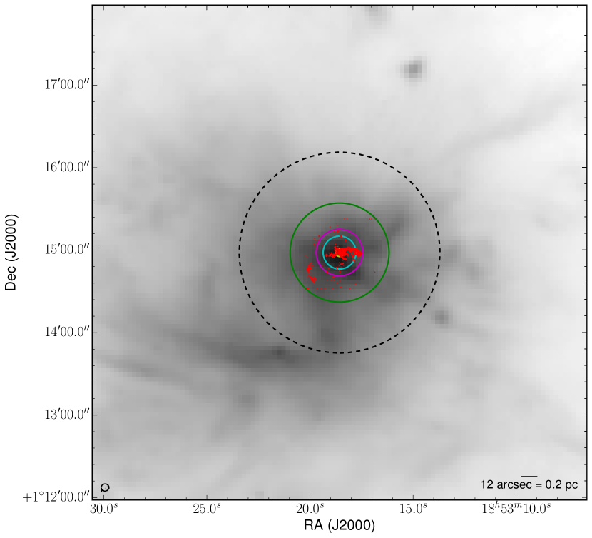
(a)

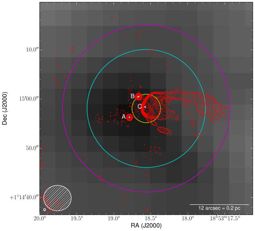
(b)

Figure 1: Far-IR grayscale image in both (a) and (b) is observed with the PACS (Photodetector Array Camera and Spectrometer, Poglitsch et al., 2010) instrument at 70 $\mu$m obtained with Herschel as part of the HOBYS Guaranteed Time key program (PI:KPGT_fmotte_1, Motte et al., 2012). It is overlaid with the contours (red) of the 2 cm free-free continuum emission observed by Sewilo et al. (2004). For the $\lambda$ = 2 cm continuum image the contour levels are at -3, 3, 5, 10, 20, 30, 40, 80, 120, 180, 250, 350, 450, 600, 800, and 850 times the noise level of 0.3 mJy beam^-1. The pixel scale of the Herschel-PACS image is 3.2$\arcsec$. The beam size of $5.2\arcsec\times 5.6\arcsec$ for the 70 $\mu$m image and $0.48\arcsec\times 0.41\arcsec$ for the 2 cm contour emission are illustrated in the lower left corner. The green, magenta and cyan circles illustrate the 36$\arcsec$, 17$\arcsec$ and 12$\arcsec$ Herschel half power beam width, at the respective frequencies 572 GHz, 1214 GHz and 1764 GHz. The circles in dashed black and yellow illustrate the model radii $R_{\rm max}$ and $R_{\rm ph}$, respectively.

We present Herschel-HIFI observations and modeling results of seven spectrally resolved ammonia transitions at THz frequencies toward the MSF region G34.26+0.15 (also known as IRAS 18507+0110, hereafter G34), in order to investigate the accretion process. These seven transitions have a high range of critical densities which made it possible for us to probe the kinematics of the different layers of G34. The source, whose properties are summarized in Table LABEL:Table:sample, is a well-studied hot core with an adjacent cluster of H₂O masers (Imai et al., 2011; Fey et al., 1994; Benson & Johnston, 1984) and OH masers (Gaume & Mutel, 1987; Garay et al., 1985), indicating the existence of an outflow at subparsec-scale (Klaassen & Wilson, 2007). In radio continuum emission, shown in Fig. 1, the source exhibits two very condensed UC H II regions called A and B, a more evolved compact H II region with a cometary shape named component C and an extended ringlike H II region called component D (Mookerjea et al., 2007; Fey et al., 1994). Component C contains a UC H II region ”head” (at which our observations were centered) and a diffuse ”tail” pointing (from tail through head) in the direction of the supernova remnant W44 (Reid & Ho, 1985). Interferometry at arcsecond resolution of molecular spectral lines, e.g., HCOOCH₃ and CH₃CH₂CN, shows that the molecular hot core emission partially overlaps with the cm-wavelength continuum emission of component C, and not with that from A and B (Mookerjea et al., 2007). Radio observations of NH₃ absorption locate the hot core between G34.26+0.15 and the observer (Heaton et al., 1989). Infall signatures of the G34 envelope have been found by Wyrowski et al. (2012) using THz observations of one ammonia transition performed with SOFIA, and modeling it using RATRAN. Our modeling, in contrast, is based upon the radiative transfer code ALI (see Sect. 5) and simultaneously reproduces seven ammonia line profiles and adjacent continuum fluxes.

Table 1: Properties of the high-mass star forming region G34.26+0.15.

$L_{\rm bol}$	$d$	$V_{\rm sys}$	$M_{\rm envelope}$	$R_{\rm envelope}$
($L_{\odot}$)	(kpc)	(km s-1)	(M⊙)	(AU)
$1.9\,\times\,10^{5}$	3.3	58.1	1800	$8.1\,\times\,10^{4}$

We present the observations and data reduction in Sect. 2 followed by results and analysis in Sects. 3 and 4, respectively. The radiative transfer modeling is presented in Sect. 5. Our modeling results are presented in Sect. 6. We discuss the results in Sect. 7 and end the paper with conclusions in Sect. 8.

2 Observations and data reduction

Table 2: Observed ammonia transitions toward G34.3$+$0.15 with Herschel-HIFI.

	Transition	Frequency	$E_{\mathrm{l}}$	$E_{\mathrm{u}}$	$A_{\rm ul}$	$n_{\mathrm{crit}}$	$g_{\rm l}/g_{\rm u}$	HPBW	$\eta_{\mathrm{mb}}$	$T_{\mathrm{C}}$	$1\sigma$/$T_{\mathrm{C}}$
	($J_{K,\epsilon}$)	(GHz)	(K)	(K)	$\log_{10}(\rm s^{-1}$)	(cm-3)		($\arcsec$)		(K)	(%)
o-NH3	1${}_{0\,+}$ – 0${}_{0\,+}$	572.498	0	27	$-$2.802	3.4e7	4/12	36	0.62	0.86	3.0
	2${}_{0\,+}$ – 1${}_{0\,+}$	1214.853	27	86	$-$1.742	3.1e8	12/20	17	0.61	4.35	2.4
	3${}_{0\,+}$ – $2_{0\,+}$	1763.524	86	170	$-$1.226	1.1e9	20/28	12	0.60	6.60	1.1
p-NH3	2${}_{1\,-}$ – 1${}_{1\,-}$	1168.452	23	79	$-$1.918	3.1e8	6/10	18	0.61	4.50	1.5
	2${}_{1\,+}$ – 1${}_{1\,+}$	1215.246	22	80	$-$1.867	3.5e8	6/10	17	0.61	4.37	2.4
	3${}_{1\,+}$ – 2${}_{1\,+}$	1763.601	80	165	$-$1.277	1.2e9	10/14	12	0.60	6.60	1.1
	3${}_{2\,+}$ – 2${}_{2\,+}$	1763.823	64	149	$-$1.482	9.3e8	10/14	12	0.60	6.60	1.1

The ground state rotational transitions of ortho-$\@element[3]{\mathrm{NH}}$, $J_{K}=1_{0}-0_{0}$ at 572 GHz, and para-$\@element[3]{\mathrm{NH}}$, $J_{K}=2_{1+}-1_{1+}$ at 1215 GHz, together with ortho-$\@element[3]{\mathrm{NH}}$ $J_{K}=2_{0}-1_{0}$ at 1214 GHz in the same band, were observed toward G34 with Herschel-HIFI in March–April 2011 as a part of the PRISMAS Guaranteed Time key program (PRobing InterStellar Molecules with Absorption line Studies). As a complement to these observations, we have observed four excited transitions of both ortho and para symmetries in April 2012 as part of our OT1 program ”Investigation of the nitrogen chemistry in diffuse and dense interstellar gas”. All observed transitions are found in Table LABEL:Table:_transitions and the Herschel observational identifications are listed in Table LABEL:Table:obsid (on-line material). The pointing for G34 was centered at $\alpha_{J2000}$ = 18^h53^m18$\aas@@fstack{s}$6, $\delta_{J2000}=+1^{\circ}$ 14$\arcmin$ 58$\aas@@fstack{\prime\prime}$0.

We used the Dual Beam Switch mode and the Wide Band Spectrometer with a bandwidth of 2.4 GHz for the highest transitions around 1764 GHz, and 4 GHz in all other bands. An effective spectral resolution of 1.1 MHz was used, corresponding to a velocity resolution of 0.2 km s^-1 for the 1764 GHz transitions, and 0.6 km s^-1 at 572 GHz. The signal was measured in horizontal and vertical polarizations, which agreed in calibrated intensity within 10 %. Because HIFI is a double side band instrument (DSB), all observations were performed with three different overlaping settings of the local oscillator (LO) to determine the sideband origin of the lines.

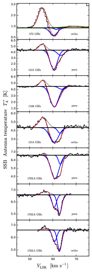
Figure 2: Single sideband spectra of all observed $\@element[3]{\mathrm{NH}}$ transitions over the LSR velocity range 45 to 75 km s^-1. The horizontal solid line represents the continuum level and the colored curves represent Gaussian fits presented in detail in Table LABEL:Table:Gaussian.

The total calibration uncertainties are $\lesssim\,$$8\,$% for band 1, $\lesssim\,$$9\,$% for band 5, and $\lesssim\,$$14\,$% for band 7, including the uncertainty in sideband gain ratio. All error components are added in quadrature. Detailed information about the HIFI calibration including errors, beam efficiency, mixer sideband ratio, pointing, etc. can be found on the Herschel internet site. The in-flight performance is described by Roelfsema et al. (2012).

The data were processed using the Herschel Interactive Processing Environment (HIPE; Ott, 2010), version 11.0 up to level 2 providing fully calibrated DSB spectra on a $T_{\mathrm{A}}^{*}$ antenna temperature intensity scale where the lines are calibrated to single sideband (SSB) and the continuum to DSB. We have accordingly divided the observed DSB continuum by two in order to be properly scaled to single sideband (SSB). The pipeline allows usage of the latest calibration and offers an alternative bandpass calibration method that smoothes optical sinusoidal standing waves occurring in band 1–5 from the internal load. It also removes standing waves at 92 and 98 MHz, which appear from the load measurements in all bands, used for intensity and bandpass calibration. The FitHifiFringe task is used to fit and remove residual ripples in the spectra using three sine functions in the frequency range 30–460 MHz. Three LO-tunings are in good agreement without any visible contamination from the image sidebands. The resulting data quality is consequently excellent with very low intensity ripples.

The FITS files are then exported to the spectral line software package xs for further analysis. Similar appearance and noise characteristics are found in all individual spectra and therefore we average all tunings and both polarizations to the final noise-weighted spectra. First-order polynomial baselines are fitted and subtracted, and as a final step the mean SSB continuum is added. All spectra in this paper are shown in a SSB intensity scale. The frequency scale is converted to Doppler velocities relative to the local standard of rest $\upsilon_{\mathrm{LSR}}$ using the line frequencies, listed in Table LABEL:Table:_transitions.

For the above line identification work we used the Jet Propulsion Laboratory, JPL (Pickett et al., 1998), catalogue entry for NH₃, which currently is based upon the extensive re-analysis of Yu et al. (2010). A review on ammonia is found in Ho & Townes (1983) and an investigation of the hyperfine structure components of the rotational transitions has been performed by Coudert & Roueff (2006) and of ortho-$\@element[3]{\mathrm{NH}}$ at 572 GHz by Cazzoli et al. (2009).

The observed spectra are shown in Fig. 2, while Fig. 3 shows the energy level diagram of ammonia with its two distinct species, ortho- and para-NH₃ (see Sect. 4.3). Note that all observed transitions have non-metastable upper states ($J_{u}>K$, $K\neq 0$), which are easily excited radiatively near luminous IR sources and have short lifetimes for radiative decay. The $J$ levels are further split in a complex hyperfine structure. However, since the $K$ = 0 ladder of energy levels has no inversion splitting, the (0,0) ground state can be studied only through the rotational $1_{0}-0_{0}$ transition at 572 GHz.

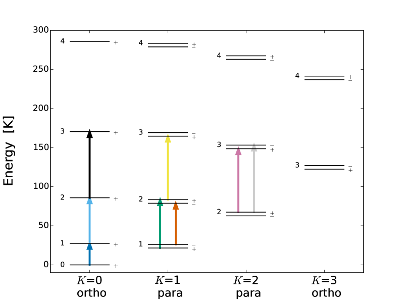
Figure 3: Energy-level diagram of $\@element[3]{\mathrm{NH}}$, where the rotational quantum number, $J$, is placed to the left of each level, the symmetry index, $\epsilon=+$ or $-$, is placed to the right of each level. The symmetry index is that defined by Rist et al. (1993), which might differ from common spectroscopic notation. The transitions are marked with colored arrows, where the direction corresponds to absorption. The gray arrow represents the 1810 GHz transition observed with SOFIA by Wyrowski et al. (2012).

3 Spectral properties

All transitions show an inverse P-Cygni profile dominated by absorption at $V_{\rm LSR}\approx 58-66$ km s^-1, except for the fundamental $1_{0}-0_{0}$ ortho transition at 572 GHz, which has a strong emission of 1.85 K and an almost saturated absorption. The 572 GHz line also shows much less absorption in the redshifted high velocity wing especially compared to the highest excited transitions at 1763 GHz. The two lowest para transitions at 1168 and 1215 GHz, both connecting to the $2_{1}-1_{1}$ state, and the $2_{0}-1_{0}$ ortho transition at 1214 GHz show similar emission of $\sim$1.2 K, but with weaker absorption in the ortho line. The highest excited $J=3-2$ transitions around 1763 GHz, with upper energy levels of 149–170 K, appear mainly in absorption. Note that even though the ortho $3_{0,+}-2_{0,+}$ and para $3_{1,+}-2_{1,+}$ transitions are separated by only 77 MHz, corresponding to 13 km s^-1, there is no overlap since the lines show absorption and emission over $\sim$11 km s^-1. The lowest transitions show broader emission and absorption features than the excited lines. The rms noise and single side band (SSB) continuum levels, $T_{\mathrm{C}}$, for all transitions are listed in Table LABEL:Table:_transitions.

The ortho 572 GHz line also shows evidence of a weak, broad and redshifted emission component not seen in any other line. In Fig. 4, we compare the line profiles of the $1_{1,0}-1_{0,1}$ ortho-H₂O Flagey et al. (2013) and the $1_{0}-0_{0}$ ortho-NH₃ transitions. Water shows a very broad emission from the source velocity up to $\sim$$150$ km s^-1 whereas ammonia, being the less sensitive to shocks and outflows, shows broad emission extending only to $\sim$$75$ km s^-1.

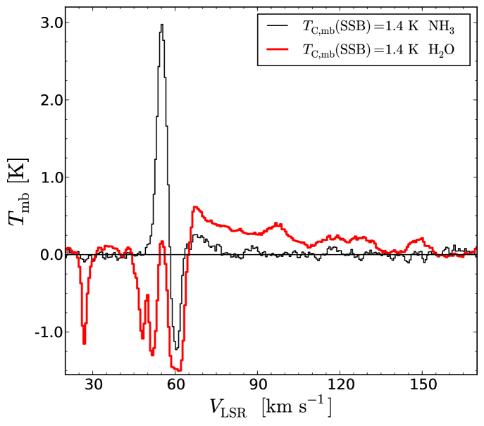
Figure 4: Comparison between o-NH₃ (572 GHz) and o-H₂O (557 GHz) Herschel-HIFI data from Flagey et al. (2013). The redshifted emission wing of water displays a clear signature of a broad outflow component from the source. Note that the water absorption is saturated around the systemic velocity ($\approx 62\leavevmode\nobreak\$km s^-1).

To allow a comparison of the absorption line profiles, all spectra are normalized as $T^{*}_{\rm A}/T_{\rm C}$ and shown in Fig. 5. The velocity at the minimum intensity increases with energy level. Together with the inverse P Cygni profiles this suggests that we are tracing gas with inward motion, confirming the results by Wyrowski et al. (2012). The different lines can thus be used to trace different layers in the absorbing gas. The critical densities are listed in Table LABEL:Table:_transitions and range from $\sim$$10^{7}$ cm^-3 for the 572 GHz transition to $\sim$$10^{9}$ cm^-3 for the highest excited lines.

We find no evidence of ammonia absorption in diffuse gas along the sight-line toward G34, in contrast to other species such as water, which shows strong foreground absorption features in the velocity range $10-55$ km s^-1 (Flagey et al., 2013).

4 Analysis

An analysis of the ammonia line profiles is not straight-forward due to the complex blend of emission and absorption features and an excitation most likely not in Local Thermodynamic Equilibrium (LTE). However, in this section we will present estimates of the velocity gradients, opacities, column density, ortho-to-para ratio and source sizes, which can be used as starting values for the more elaborate modeling in Sect. 5 using an Accelerated Lambda Iteration code.

4.1 The absorbing material

4.1.1 Velocity gradients

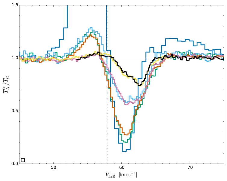
Figure 5: Normalized spectra of all observed $\@element[3]{\mathrm{NH}}$ transitions used in the analysis of the absorption line profiles (same color code as in Fig. 3). The vertical black dotted line marks the systemic velocity of G34.

To quantify the velocity gradient, the lower state energies of all transitions are plotted in Fig. 6 as a function of the $V_{\mathrm{LSR}}$ of the minimum absorption line intensities. Comparing the result of minimum intensity measured directly from observed spectra and from gaussian fits of two absorption profiles (Table LABEL:Table:Gaussian), we find that the lines cluster around two velocities, $\sim$60.6 and $\sim$63.0 km s^-1, suggesting the existence of two gas components moving inwards toward the center of the cloud, each with approximately constant velocity. The lines of highest excitation, 1763.5 GHz (ortho) and 1763.6 GHz (para), have negligible emission and thus trace the absorption velocities rather accurately with a minimum intensity at $\sim$63.0 km s^-1 although they also display absorption at lower velocities. The lines of intermediate excitation, 1214 (ortho) and 1763.8 GHz (para), show approximately equal absorption in both velocity components, whereas the lowest ortho- and para-lines at 572, 1168 and 1215 GHz mainly show absorption at $\sim$60.6 km s^-1. The velocities at the minimum intensity in these lines are more uncertain due to their stronger emission, in particular the 572 GHz line. However, since the 1168, 1215 and 1214 GHz lines have very similar emission over $V_{\mathrm{LSR}}\approx 51-58$ km s^-1, and the 1214 and 1763.8 GHz lines also have almost identical absorption line profiles over $V_{\mathrm{LSR}}\approx 58-66$ km s^-1 (with emission only in the 1214 GHz line), the peaks of emission and absorption are sufficiently well separated that the absorption velocities are well determined.

4.1.2 Optical depth and column density

In order to parameterize the spectral lines, we have performed multicomponent Gaussian fits to all lines (see Fig.2). We list the results in Table LABEL:Table:Gaussian and display the fits in Fig. 2. For the 572 GHz transition, an additional component corresponding to the broad emission line was included.

Table 3: Results from Gaussian fits, $T_{\rm l}$, $\Delta V$, and $V_{\mathrm{LSR}}$ for the emission, calculated peak opacities, $\tau_{\mathrm{p}}$, integrated opacities, $\int\tau_{\nu}dV$, and column densities of the absorbing material in respective lower state, $N_{\mathrm{l}}$.

	Freq	$T_{\rm l}$	$\Delta V$	$V_{\mathrm{LSR}}$	$\tau_{\mathrm{p}}$	$\int\tau_{\nu}dV$	$N_{\rm l}$
	(GHz)	(K)	(km s-1)	(km s-1)		(km s-1)	($\rm cm^{-2}$)
o-NH3	572.498	$-0.7\pm 0.1$	$3.8\pm 0.3$	$60.3\pm 0.3$	1.3	5.4	2.0e13
		$-0.1\pm 0.1$	$2.1\pm 0.9$	$61.4\pm 0.3$	0.2	$\lesssim$0.4	$\lesssim$1.5e12
		$1.85\pm 0.01$	$4.2\pm 0.07$	$55.55\pm 0.04$		…	…
		$0.14\pm 0.01$	$10.0\pm 0.8$	$69.5\pm 0.3$		…	…
	1214.853	$-1.7\pm 0.1$	$4.5\pm 0.9$	$60.5\pm 0.4$	0.5	2.3	1.3e13
		$-0.6\pm 0.4$	$2.4\pm 0.7$	$63.1\pm 0.3$	0.2	$\lesssim$0.4	$\lesssim$2.2e12
		$1.2\pm 0.1$	$4.3\pm 0.4$	$55.9\pm 0.3$		…	…
	1763.524	$-0.92\pm 0.2$	$2.2\pm 0.5$	$60.8\pm 0.1$	0.2	0.4	2.2e12
		$-1.7\pm 0.1$	$2.2\pm 0.1$	$62.8\pm 0.1$	0.3	0.7	4.1e12
		$0.10\pm 0.08$	$4.2\pm 18$	$56.8\pm 6.7$		…	…
p-NH3	1168.452	$-3.2\pm 0.1$	$4.3\pm 0.3$	$60.6\pm 0.1$	1.3	5.7	4.2e13
		$-0.4\pm 0.3$	$3.1\pm 0.7$	$63.8\pm 0.6$	0.1	$\lesssim$0.3	$\lesssim$2.6e12
		$1.03\pm 0.04$	$3.1\pm 0.2$	$55.8\pm 0.1$		…	…
	1215.246	$-3.3\pm 0.3$	$4.3\pm 0.3$	$60.4\pm 0.2$	1.4	5.4	4.0e13
		$-0.9\pm 0.6$	$3.1\pm 0.7$	$63.5\pm 0.8$	0.2	$\lesssim$0.9	$\lesssim$6.6e12
		$1.07\pm 0.04$	$3.5\pm 0.3$	$55.8\pm 0.1$		…	…
	1763.601	$-1.04\pm 0.05$	$2.3\pm 0.2$	$60.6\pm 0.2$	0.2	0.4	2.8e12
		$-1.60\pm 0.05$	$2.2\pm 0.1$	$62.9\pm 0.2$	0.3	0.6	4.4e12
		$0.29\pm 0.02$	$3.9\pm 0.8$	$56.8\pm 0.2$		…	…
	1763.823	$-2.85\pm 0.04$	$4.1\pm 0.2$	$60.9\pm 0.1$	0.6	2.5	2.7e13
		$-1.1\pm 0.2$	$2.0\pm 0.2$	$63.3\pm$0.1	0.2	0.4	4.2e12
		$0.27\pm 0.04$	$1.7\pm 0.4$	$56.2\pm 0.1$		…	…

We calculate the integrated optical depth for the absorption components obtained from the Gaussian fits as

$$\int\tau_{\nu}\,\mathrm{d}V\approx 1.06\,\tau_{\mathrm{p}}\,\Delta V\approx-1.06\,{\rm ln}\,\bigg{(}1-\frac{|T_{\rm l}|)}{T_{\rm C}}\bigg{)}\,\Delta V\ ,$$ (1)

where $\tau_{\mathrm{p}}$ is the peak opacity, $\Delta V$ is the line width, $|T_{\rm l}|$ is the absolute value of the amplitude of the Gaussian fit, and $T_{\rm C}$ is the sum of the continuum and the emission contribution to the continuum, $T_{\rm C}({\rm EM})$, which is estimated using the gaussian emission profile (Table LABEL:Table:Gaussian). Assuming that ammonia and water co-exist, we use the fact that the water line shows saturated absorption at the zero level to support our underlying assumption in Eq. 1 that the absorbing material completely covers the background continuum within the beam.

The ammonia line profiles exhibit a mixture of emission and absorption in the presence of a strong submm-wave continuum. Such spectra suggest that the radiating envelope is stratified and that it contains gaseous molecules like $\@element[3]{\mathrm{NH}}$ mixed with dust. The continuum radiation is intense; for example, $T_{\rm b}=4.4$ K at 1215 GHz corresponds to a surface brightness $I_{\nu}=3.3\times 10^{-15}$ W m^-2 Hz^-1 sr^-1 averaged over the 17$\arcsec$ Herschel beam. This means that the absorption rate in the $2_{1\,+}\leftarrow 1_{1\,+}$ transition is

$$I_{\nu}B_{\rm\ell,u}=2.4\times 10^{-3}\;\;\;[{\rm s}^{-1}]\;,$$

where $B_{\rm\ell,u}$ is the Einstein coefficient for absorption. In comparison with the rate coefficient for collisional excitation in the same transition at a collision temperature of 50 K, $C_{21}=4.0\times\,10^{-11}$ cm³ s^-1 (Danby et al., 1988), a hydrogen density of $n({\rm H}_{2})=6.0\times 10^{7}$ cm^-3 would be required for collisions to compete with radiative processes (cf. the critical density for emission in Table LABEL:Table:_transitions). Consequently, the excitation of $\@element[3]{\mathrm{NH}}$ is probably not in LTE and thus requires analysis by means of a non-LTE radiative transfer model of a dynamical envelope.

Although the continuum radiation of G34 is non-negligible for radiative excitation in the full non-LTE treatment of NH₃, the resulting excitation temperatures do not significantly change the results of the simple analysis. We have here neglected the contribution of emission assuming that $J(T_{\mathrm{ex}})\,$=$\,h\,\nu/k\times(\exp(h\,\nu/(k\,T_{\rm ex}))-1)^{-1}\ll T_{\mathrm{C}}$, and that the cosmic microwave background (CMB), is negligible at the frequencies considered here (¡1.5 mK).

Using the simple analysis, the column densities of respective lower state can now be calculated with

$$N_{\rm l}\,=\,8\pi\frac{g_{\rm l}}{g_{\rm u}}\frac{\nu^{3}}{c^{3}}\frac{\int\tau_{\nu}dV}{A_{\rm ul}}\frac{1}{1-{\rm exp}(-\frac{h\nu}{kT_{\rm ex}})}\approx\,8\pi\frac{g_{\rm l}}{g_{\rm u}}\frac{\nu^{3}}{c^{3}}\frac{\int\tau_{\nu}dV}{A_{\rm ul}}\ ,$$ (2)

where $g_{\rm l}/g_{\rm u}$ is the ratio of the degeneracy factors of the lower and upper levels and $A_{\rm ul}$ is the Einstein coefficient for spontaneous emission. The degeneracy factors and the Einstein coefficients are listed in Table LABEL:Table:_transitions.

A lower limit to the total ammonia column density in the absorbing material then is found by summing all $J=0$, 1 and 2 lower state column densities listed in Table LABEL:Table:Gaussian

$$N_{\rm tot}=\sum N_{\rm l}\geqslant 2.1\times 10^{14}\,\,\,[\rm cm^{-2}]\ .$$

In the above summation we have also added the two unobserved para transitions 3${}_{2\,-}\leftarrow 2_{2\,+}$ (at 1810 GHz) and 3${}_{1\,+}\leftarrow 2_{1\,-}$ (1809 GHz) by counting our observed 3${}_{2\,+}\leftarrow 2_{2\,+}$ and 3${}_{1\,+}\leftarrow 2_{1\,+}$ columns twice since their intensities are expected to be similar. The 1810 GHz line was observed by Wyrowski et al. (2012), who confirm our estimated intensity. The total column density can be higher if higher levels than $J=2$ are populated. At cm wavelengths the (3,3) inversion line can for instance be rather strong indicating non-negligible population of this level.

Figure 6: Lower state energies plotted as a function of $V_{\rm LSR}$ (a) at the minimum intensity and (b) at the minimum intensity of the Gaussian fits of the two absorption profiles (see Table LABEL:Table:Gaussian). The strong emission and weak absorption at higher velocity may explain the low $V_{\rm LSR}$ for the 572 GHz line. Same color code is used as in Fig. 3.

Neglect of emission in the submm lines causes the total column density to be underestimated by a factor of two, based on the excitation temperatures (at $r=R_{\rm max}$) computed in our best-fitting non-LTE models (see Sect. 5 and Fig. 11) and $\tau=-\ln{(|T_{\rm l}|-J(T_{\rm ex}))/(T_{\rm C}+T_{\rm C}({\rm EM})-J(T_{\rm ex}))}$.

4.2 Size estimates

Our $1_{0}-0_{0}$ spectrum can also be compared to observations of this transition performed with the Odin satellite (Nordh et al., 2003) toward G34 (Hjalmarson et al., 2005). Fig. 7 shows the comparison. The ratio of the Herschel and Odin antenna temperatures gives an estimate of the sizes of the emission and continuum components according to

$$\frac{T^{*}_{\rm A,Herschel}}{T^{*}_{\rm A,Odin}}=\frac{\eta_{\rm mb,Herschel}}{\eta_{\rm mb,Odin}}\times\frac{\theta_{\rm s}^{2}+\theta_{\rm mb,Odin}^{2}}{\theta_{\rm s}^{2}+\theta_{\rm mb,Herschel}^{2}}\ ,$$ (3)

where $\theta_{\mathrm{s}}$ is the effective circular Gaussian source size in arcseconds, $\eta_{\mathrm{mb,Odin}}=0.9$, and $\theta_{\rm mb,Odin}=126$″, at 572 GHz.

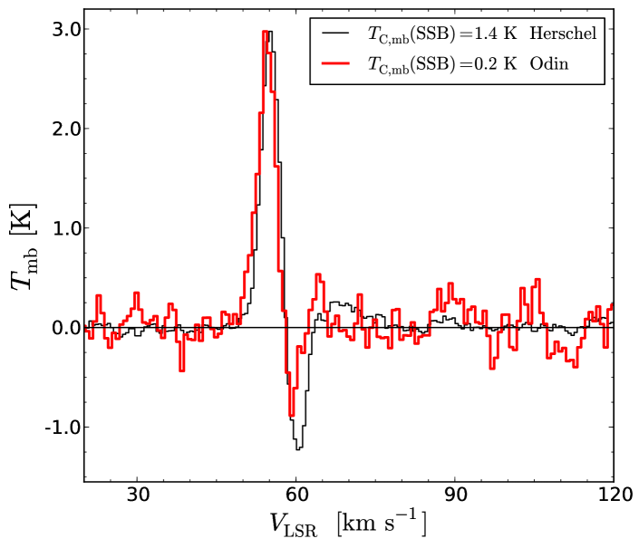
Figure 7: Odin and Herschel observations of ortho-$\@element[3]{\mathrm{NH}}$ 1₀ – 0₀ at 572 GHz. The continuum levels, noted in the legend, are subtracted and the Odin spectra is scaled up with a factor of 7, to allow a comparison of the spectra.

The resulting mean source sizes are comparable to the 36″  Herschel beam, $\sim 35\arcsec$ and $\sim 38\arcsec$ for the narrow emission and the continuum, respectively. This supports the assertion that it is the dust, mixed with the emitting gas, that is responsible for the major part of the continuum emission. The size of the broad emission is derived using the Odin noise level as 1$\sigma$ ($\sim$29 mK) upper limit, which we find to be $\lesssim 34\arcsec$. Small variations of the ratio of antenna temperatures have, however, a high impact on the derived sizes. A 20% calibration uncertainty in both spectra gives for instance an error of $\pm 20\arcsec$.

4.3 Ortho-to-Para ratio

Two possible relative orientations of the hydrogen spins create two distinct species: ortho-$\@element[3]{\mathrm{NH}}$ (all spins are parallel, $K$ = 3$n$ where $n$ is an integer $\geq 0$) and para-$\@element[3]{\mathrm{NH}}$ (not all H spins are parallel, $K\neq 3n$). Rotational transitions normally are not allowed between ortho and para states. Neither can radiative or non-reactive collisional transition change the spin orientation between the two symmetries, once formed. Measurements of the ortho-to-para ratio (OPR) can give valuable insights into the competing processes of formation and destruction, radiative and collisional excitation, and reactive interchange processes in interstellar space.

Ammonia formation in the gas-phase at high temperatures is expected to result in OPR ratios close to the statistical value of one, because the energy release in the formation process is much higher than the energy difference between the lowest para and ortho states (22 K). If ortho-NH₃ is formed or condensed at low temperatures (¡30 K) on water ice covered dust grains and then desorbed when the grain is heated to 100 K, the OPR may be higher than one.

Our new observations and analysis of three ortho and three para lines probing different energies can for the first time be used to estimate the OPR in dense ($10^{4}$ ¡ $n_{\rm H_{2}}$ ¡ $10^{7}$ cm^-3) and warm (15 ¡ T ¡ 100 K) gas in star-forming regions. Using the results from Table LABEL:Table:Gaussian we find

$$N(\mathrm{ortho})=\sum N_{\rm l}(\mathrm{ortho})\geqslant 0.43\times 10^{14}\,\,\,[\rm cm^{-2}]\ ,$$

and

$$N(\mathrm{para})=\sum N_{\rm l}(\mathrm{para})\geqslant 1.68\times 10^{14}\,\,\,[\rm cm^{-2}]\ ,$$

that gives us an OPR$\sim$0.3 in the absorbing material, below unity.

This result takes into account all levels of $J<3$ and $K<3$, but not the $J\geqslant 3$ levels, which may be populated. Since the ($J,K$)=(3,3) levels would be proportionally most populated, the effect of omitting higher level populations in this OPR estimate makes it effectively a lower limit. However, as will be shown with non-LTE radiative transfer models (below), the computed population in the (3,3) levels account for at most 10% and $10^{-4}$% of the total population in the innermost and outermost region, respectively. The inclusion of these levels could no more than double the estimated OPR. Thus, the indication of an OPR less than unity is quite secure even considering the effects of excitation.

5 Spherical non-LTE models

Our basic analysis (in Sect. 4.1.2) already suggests that the $T_{\rm ex}$ is different for different transitions, and therefore it is important to perform non-LTE modeling. In order to construct an accurate model that properly accounts for the line overlap and coupling to the continuum, we adopt a non-LTE, one-dimensional, radiative transfer model based on the accelerated lambda iteration (ALI, Rybicki & Hummer, 1991, 1992) method. ALI solves the coupled problem of radiative transfer and statistical equilibrium from an initial guess of the level populations. The code we employed has been used by Wirström et al. (2010), Bjerkeli et al. (2011), and was benchmarked by Maercker et al. (2008), where the technique is described in more detail.

Given the complexity of the MSF region, the locations and sizes of the HIFI submm-wave beams are plotted relative to the entire structure in Fig. 1. The two smallest HIFI-beams (cyan and magenta) cover the densest part of the complex region emitting at 70 $\mu$m, overlapping component A, B and the head of component C. The largest beam (green) in addition includes the less dense and non-symmetric far-IR region. Fig. 1 also illustrates the size of the modeled spherically symmetric source and its inner IR-continuum object. Considering that the model is spherically symmetric and that the region contained within the HIFI submm-wave beams exhibits enormous complexity, it does give a useful representation of the molecular envelope over the scale of the projected beam.

The physical properties of the spherically symmetric model, like density and temperature, can be varied over a number of homogeneous shells, which move radially at a given velocity (Sect. 5.1). An ensemble of models is constructed for a range of fixed and varying input parameters in a large grid (Sect. 5.2). The best-fitting model is identified by minimizing the difference between observed and computed spectral line profiles (Sect. 5.3), and by requiring that the continuum is reproduced to within 10% (Sect. 6).

5.1 Procedure

The number of shell-like cells and angles used in the ray-tracing can be arbitrarily chosen. In the present work, typically 40 shells and 32 angles are used. Fig. 8 shows an illustration of the model and how the collapsing cloud produces an inverse P-Cygni line profile. The ALI code produces an adjacent continuum for each shell, throughout the cloud. The centrally peaked hot dust distributions and the dust in the extended envelope emit strong infrared continuum radiation, which has a great influence on both line shapes and intensities. The computed intensities are convolved with appropriate antenna beam response functions for direct comparison with observed line profiles, corrected for beam efficiencies.

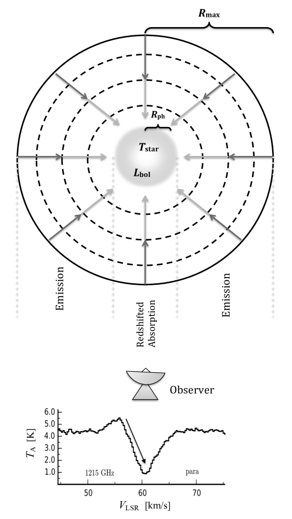
Figure 8: Sketch illustrating the spherical ALI model with shells, an inner source, and two velocity fields in the contracting envelope. The absorption feature is due to the redshifted part of the envelope in front of the strong continuum from the H II region and the hot dust throughout the gas cloud.

Our observed NH₃ line profiles show components with line widths of a few km s^-1 (cf. Table 3). The hyperfine splitting (hfs) is about 3 MHz, which corresponds to 1.5 km s^-1 for the $1_{0}-0_{0}$ line. We have therefore used spectral line data, which include the hfs splitting to generate model spectra of overlapping hfs transitions. However, collisional cross sections between hfs levels are not available for NH₃. For collisional rates, we take hfs splitting into account approximately by adopting the method outlined in Alexander & Dagdigian (1985) where cross sections between hfs levels can be related to purely rotational cross sections along a rotational ladder. As basic cross sections we here used those of Danby et al. (1988), which include levels $J\leq 6$ (those of Maret et al. 2009 only include $J\leq 3$).

Radiation

The radiation field consists of the infrared continuum radiation from the dust, the central source, and the cosmic microwave background. The central source represents the dust photosphere separating the inner region, where diffusion determines the temperature gradient, from the outer region, where balance between heating and cooling determines the dust temperature. The input parameters specifying the dust continuum are the dust temperature ($T_{\rm dust}$), the emissivity parameter ($\kappa_{250\mu m}$), the frequency dependence of the dust emissivity ($\beta$), and the gas-to-dust mass ratio. The infrared heating from the central source is defined by the dust photosphere’s effective temperature ($T_{\rm star}$) and luminosity.

The spectral energy distribution (SED) and the physical structure of G34 were modeled by van der Tak et al. (2013) based on sub-millimeter continuum maps. We adopt their resulting bolometric luminosity and source size to estimate the infrared continuum radiation from the central source. The gas temperature is to a first approximation set to be equal to the dust temperature, which holds very well for the inner part with its high densities, and lies within the uncertainties for the outer part. The power law exponent, $q$, in $T=T_{0}\,r^{-q}$ K for the radial temperature profile is adopted from a model made by Garay & Rodriguez (1990) for molecular gas that ranges from a few hundredths of parsecs to a few parsecs, based on NH₃ observations at high resolution ($3\arcsec$, eight times smaller than the smallest Herschel beam illustrated in Fig. 1). It is then varied together with the temperature in the outermost shell at $R_{\rm max}$, $T_{0}$, and the source size in order to reproduce the observed continuum within 20%, but also the absorptions in the data.

Density profile

Massive hot cores are embedded in cooler, lower density and more extended structures that are likely to be highly fragmented into filaments and dense clumps. Therefore the physical conditions derived assuming smooth density profiles should be taken only as representative of the bulk conditions of the clumpy emitting region.

Two cases of radial density profile are modeled. The first contains two zones, where the inner zone has constant density. The outer zone has a power-law dependence on radial distance $n=n_{0}\,r^{-p}$ cm^-3, in which $n_{0}$ (the density at $R_{\rm max}$) and $p$ are free parameters. The range of densities explored thus encompasses the various densities inferred in previous work by van der Tak et al. (2013), Garay & Rodriguez (1990), Matthews et al. (1987) and Heaton et al. (1985) and includes the possibilities of having a tenuous foreground cloud or a dense extended envelope or halo. Both the boundary radius and the constant density are used as free parameters. The density profile for the second case assumes $n$ to increase continuously all the way towards the center.

Abundance structure

At low gas-phase temperatures, molecules are expected to stick to the surfaces of dust grains upon collision, building up mantles dominated by water ice. Closer to MYSOs where the temperature is higher these ices start to evaporate. Since most NH₃ molecules are trapped in the water ice matrix, the bulk of ammonia will be released into the gas-phase at temperatures above 100 K, when water itself evaporates. In the cold outer envelope, where $T<T_{\rm evap,\,\rm NH_{3}}$, the $\@element[3]{\mathrm{NH}}$ abundance profile is governed by reactions in the gas phase. As a result, the $\@element[3]{\mathrm{NH}}$ abundance is likely to vary in a complicated way. Therefore, the fractional abundance of ammonia, $X$(NH₃) = $n$(NH₃)/$n$(H₂), is set to be a free parameter in a step profile (details in Sect. 5.2).

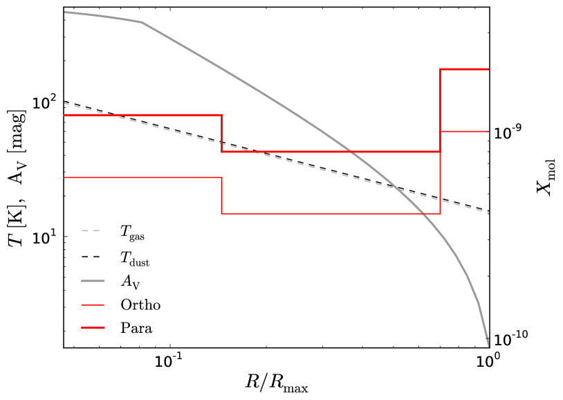
Figure 9: Models best-fit profile for the abundance of ortho and para NH₃ and the temperature, are displayed as a function of the normalized radius of the cloud. The visual extinction, $A_{\rm V}$, is proportional to the radial integral of the total hydrogen density and is displayed here as increasing from the outer boundary inwards.

Velocity structure

For comparison, four different infalling velocity fields are explored where the velocity of the center is taken to be 58.1 km s^-1 : (i) two velocity regimes, each moving with a constant velocity corresponding to the center velocities of the two absorption components distinguished in Fig. 6, both allowed to vary over $\pm$1 km s^-1 in steps of 0.1 km s^-1 around the mean $V_{\rm LSR}$ of the Gaussian fits in Table LABEL:Table:Gaussian (60.6 and 63.0 km s^-1). The radius at which the two velocity fields border is described in Sect. 5.2; (ii) one velocity regime in free-fall similar to the modeling by Wyrowski et al. (2012) and Rolffs et al. (2011) who used a free-fall-fraction of $f=0.3\pm 0.1$. The free-fall velocity is related to the mass interior to radius $r$, $M_{\rm in}$, the radius at which infall begins, $a$, and scaled by the parameter $f$:

$$\varv=-f\times\sqrt{2GM_{\rm in}\bigg{(}\frac{1}{r}-\frac{1}{a}\bigg{)}},$$ (4)

where $G$ is the gravitational constant. The mass $M_{\rm in}$ includes both the mass of the central MYSOs, $M_{0}$, which is a free parameter (see Sect. 5.2), and the interior mass of the collapsing cloud; (iii) two velocity regimes in free-fall, where $f=0.6\pm 0.2$ for the inner velocity field and $f=0.3\pm 0.2$ in the outer. The radius at which the two velocity fields border and the radius at which the collapse starts are described in Sect. 5.2 ; and, (iv) three velocity regimes, where the inner two velocity components are constant and described in (i) above, and the outer component is in free-fall, where $f=0.3\pm 0.2$. The radius at which the velocity fields border and start to collapse are described in Sect. 5.2. No attempt has been made to incorporate a broad, redshifted component to reproduce the broad, weak emission feature in the 572 GHz line.

5.2 Grid of models

We hold the following parameters fixed and constant through the modeled cloud: $d_{\rm source}$, $V_{\rm LSR}$, $L_{\rm bol}$, the gas-to-dust ratio, $\kappa_{250\mu m}$ and $\beta$ as given in Table LABEL:Table:model.

Table 4: Parameter values or profile of the best-fit ALI model and results.

Parameters held constant
Distance to source, $d_{\rm source}$	3.3	[kpc]
$V_{\rm LSR}$	58.1	[km s-1]
Envelope size, $R_{\rm max}$	$1.8\times 10^{18}$	[cm]
IR-continuum size, $R_{\rm ph}$	$7.1\times 10^{16}$	[cm]
Luminosity of source, $L_{\rm bol}$	$1.9\times 10^{5}$	[L⊙]
IR-temperature, $T_{\rm star}$	120	[K]
Gas-to-dust ratio, $M_{\rm gas}/M_{\rm dust}$	100
Emissivity parameter, $\kappa_{250\mu m}$	20	[cm2 g-1]
Dust frequency dependence, $\beta$	1.8
Ortho to para ratio, OPR	0.5
Parameters profile
Gas temperature, $T_{\rm g}$	$15.0\,r^{-0.61}$	[K]
Dust Temperature, $T_{\rm d}$	$1.03\times T_{\rm g}$	[K]
H2 density, $n(\rm H_{2})$
$r<0.075$	$2.3\times 10^{6}$	[cm-3]
$r>0.075$	$1.8\times 10^{4}\,{r}^{-2.3}$	[cm-3]
Velocity profile, $\varv_{\rm infall}$
$r<0.2$	5.3	[km s-1]
$0.2<r>0.7$	2.7	[km s-1]
$r>0.7$	$\left\{\begin{tabular}[]{l}$f$ = 0.3\\ $M_{0}=1$\\ $a=1$\end{tabular}\right.$	[M⊙]
Micro turbulence, $\varv_{\rm turb}$
$r<0.9$	1.0	[km s-1]
$r>0.9$	1.6	[km s-1]
Abundance, $X(\mathrm{NH}_{3})$
$r<0.145$	$1.2\times 10^{-9}$
$0.145<r<0.7$	$0.8\times 10^{-9}$
$r>0.7$	$2.0\times 10^{-9}$
Results
$N(\rm p$-$\mathrm{NH}_{3})$	$9.1\times 10^{14}$	[cm-2]
$N(\rm o$-$\mathrm{NH}_{3})$	$4.6\times 10^{14}$	[cm-2]
$N(\mathrm{H}_{2})$	$8.4\times 10^{23}$	[cm-2]
$M$(G34)	2 700	[M⊙]
$\dot{M}_{\mathrm{acc}}$
$r=R_{ph}$	$4.1\times 10^{-3}$	[M⊙ yr-1]
$r=0.075R_{max}$	$4.5\times 10^{-2}$	[M⊙ yr-1]
$r=0.2R_{max}$	$1.7\times 10^{-2}$	[M⊙ yr-1]
$r=0.7R_{max}$	$4.5\times 10^{-3}$	[M⊙ yr-1]

We vary the envelope size, $R_{\rm max}$, and the effective IR-temperature of the star, $T_{\rm star}$, to find the best combination before we hold these values constant. For a fixed luminosity, the size and stellar temperature can vary: the higher the value of $T_{\rm star}$, the smaller the value of $R_{\rm ph}$, and vice versa. Values of $T_{\rm star}$ between 70 and 1000 K were tested. The range of maximum envelope sizes was $1\times 10^{18}$ to $3\times 10^{18}$ cm. This range includes the sizes estimated by van der Tak et al. (2013) and Rolffs et al. (2011) as well as the radius derived from the comparison of Odin and Herschel measurements at 572 GHz ($\S$4.2). The continuum radiation from mm to infrared wavelengths stems from heated dust grains.

The following parameters have a profile structure through the cloud that is varied:

• Temperature: $T_{0}$, in $T\,$=$\,T_{0}\,{r}^{-q}$, is varied between 5 and 30 K, in steps of 2 K, and $q$, is varied $0.6\,\pm$0.2 in steps of 0.01.

• Density: $(i)$ continuous profile: $p$, in $n\,$=$\,n_{0}\,{r}^{-p}$, is varied between 1.5 and 2.5 in steps of 0.1 along with $n_{0}$, which is allowed to vary between $10^{3}$ and $10^{5}$ cm^-3. $(ii)$ Inner profile: the boundary radius and the density are varied, between 0.05$R_{\rm max}$ and 0.1$R_{\rm max}$ and between $10^{5}$ and $10^{8}$ cm^-3, respectively. Outer profile: is the same as the continuous profile.

• Abundance: (i) Values between $10^{-10}$ and $10^{-7}$ are varied as a free parameter in a constant profile through the whole cloud. (ii) Same range of abundance is used to vary for a two and three-step profile, where the radius at each step is varied as a free parameter. The OPR for any profile is varied between 0.3 and 1.0.

• Velocity: (i) For the two and three velocity regimes profile the intersecting radius is varied between 0.04$R_{\rm max}$ and 0.9$R_{\rm max}$, with steps of 0.01$R_{\rm max}$. (ii) For a free-fall collapse the mass of the UC H II region is varied between 1 and 2000 M_⊙. The collapse is assumed to be initiated at $a=R_{\rm max}$.

• Micro turbulence: $(i)$ A constant $\varv_{\rm turb}$ profile is set through the whole cloud and varied between 0.5 and 2 km s^-1. $(ii)$ A step profile with a constant inner and outer $\varv_{\rm turb}$ is varied together with the boundary radius, as free parameters. The profile in the outer envelope is set to a higher value compared to the inner, as measured by Liu et al. (2013); Coutens et al. (2014) for G34 and by Herpin et al. (2012); Caselli & Myers (1995) for other massive protostars.

5.3 Uncertainties of the parameters

We use the chi-square ($\chi^{2}$) method to get a statistical comparison of the qualities of fits. For each line and model we compute

$$\chi^{2}_{\rm line}=\sum^{n_{\rm ch}}_{i=1}\frac{(o_{i}-m_{i})^{2}}{\sigma^{2}}$$ (5)

where $n_{ch}$ is the number of channels between $V_{\mathrm{LSR}}=54$ and 68 km s^-1 where the absorption is located for all lines and models. $o_{\rm i}$ and $m_{\rm i}$ are the observed and modeled continuum subtracted intensities, respectively. The observational error is dominated by calibration uncertainties (assumed to be 14 %, thus representing the band with the highest quadratic combination of noise presented in Sect. 2) rather than by thermal noise that is $<$10 %. Therefore $\sigma$ represents the calibration uncertainty multiplied with the maximum intensity, $T_{\rm mb}(\rm max)$, in the spectra (with continuum, $T_{\rm C,\rm mb}$). This method is adopted from Rolffs et al. (2011). To compare the models we sum $\chi^{2}_{\rm line}$ over all transitions, except for the 572 GHz transition since we have limited possibilities to model the broad redshifted emission with ALI. The model with the lowest value of $\sum{\chi^{2}_{\rm line}}$ determines the best-fit model. A model is assumed to successfully reproduce the observed line profile if the continuum intensity of the best-fit model is within 20% of the observational value.

6 The best-fit model

The physical parameters of the best-fitting model are presented in Table LABEL:Table:model. The line profiles and continuum fluxes of this model are compared with the observed spectra in Fig. 10. The robustness of the model is discussed in Sect. 6.1. The models used to describe G34 by Wyrowski et al. (2012) and Coutens et al. (2014) are discussed and compared with the best-fit model in Sect. 6.2.

Six of the absorption line profiles in Fig. 10 are very well reproduced between $V_{\mathrm{LSR}}$ = 60 and 66 km s^-1. Two of the emission line profiles are, however, somewhat overestimated, but one could expect a perfect match only if the observed region were more uniform and unstructured within the projected beam. How well the model is able to reproduce the observed continuum level is shown in the lower right corner of each spectrum, for the best-fit model always within 10%. It is a challenge to model the fundamental ortho 572 GHz line simultaneously with the higher excited transitions. Both too little emission and too little absorption are found, which is speculated to be due to the one-dimensional spherical symmetry of the model but also our assumed simplifications of the source structure, as further explained in Sect. 7.1.

There is evidence of gradients in the density, gas and dust temperature, micro turbulence and ammonia abundance, within the inflowing molecular gas associated with G34. The scale of the gradient from observational data, is between 0.2 pc (with the best resolution being 12$\arcsec$ at 3.3 kpc) and 0.6 pc (36$\arcsec$ at 3.3 kpc). For the best-fit model it stretches longer, between 0.023 pc and 0.583 parsec. Garay & Rodriguez (1990) proposed a physical structure of ammonia, based on interferometric observations at cm wavelengths, which shows that the best-fit model probes a region between a Hot ultra-compact core and a Molecular core.

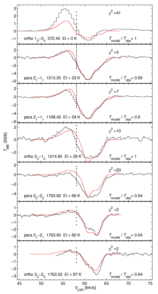
Figure 10: Three velocity regimes with two inner constant profiles and an outer free-fall profile. The inner and outer constant velocity profiles have a velocity of 5.3 and 2.7 km s^-1, respectively, and the free-fall profile uses $f$ = 0.3, $M_{0}=1$ M_⊙ and $a$ = 1. Observed Herschel-HIFI spectra in black compared to the best-fitting model line profiles in red. The ratio of the modeled and observed continuum at the frequency of each line is given in respective legend. The vertical black dotted line marks the systemic velocity of G34. $\sum{\chi^{2}_{\rm line}}$ = 46 , over $\Delta V_{\mathrm{LSR}}=54-68$ km s^-1.

6.1 Parameters

Temperature profile

The modeled $T_{\mathrm{ex}}$, $T_{\mathrm{K}}$ and $n(\mathrm{H_{2}})$ are plotted as functions of normalized radius in Fig. 11. The difference between excitation temperature and kinetic temperature is the result of departures from LTE throughout the envelope. This shows that the density is too low for collisional excitation to dominate over radiative processes.

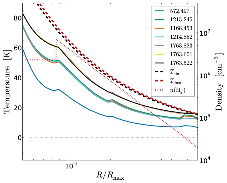
Figure 11: Excitation temperatures in the best-fitting model as a function of the normalized radius. The gas temperature, $T_{\rm g}$, dust temperature, $T_{\rm d}$, and density, $n$(H₂), are also plotted for comparison. We use the same color code as in Fig. 3.

Density profile

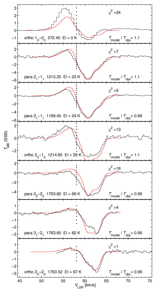
Figure 16: ALI: Three velocity regimes as in the best-fit model (Fig. 10) with a radial continuous density profile. Notation as in Fig. 10. $\sum{\chi^{2}_{\rm line}}$ = 50.

The combined emission and absorption profiles are well reproduced by a step-wise density profile, which permits two distinct infall velocities to be included. The best-fitting model has a central flattening of the density distribution joined to a power-law profile that decreases outwards. Adoption of a continuous density profile throughout the envelope results in a somewhat poorer fit ($\sum{\chi^{2}_{\rm line}}$ increases from 46 to 50), with excess absorption in the 1214 and 1763.6 GHz lines and excess continuum near all lines. An example of a continuous model is shown in Fig. 16. The central flattening in our best-fit density profile, illustrated in Fig.11, is located at $<$0.04 pc. An increase of the radius of this region decreases the emission, absorption and continuum for all the lines (especially for the lines of highest excitation) and vice versa when decreasing its radius.

The flat and lower density profile for the inner envelope, of $\lesssim 9000$ AU, can be explained by:

1. A disc of molecular gas that is formed from the collapse of a massive, rotating fragment embedded in an extended molecular cloud as suggested by Garay & Rodriguez (1990) and Garay et al. (1986). The size of the possible disc ($\lesssim 9000$AU) agrees well with estimated sizes of disks associated with young massive objects (single protostars or clusters) showing signs of outflows but no jets (Garay & Lizano, 1999).

2. The relation between the inner envelope and the contraction process of gas and dust, causing the disk to spin-up to high velocity gradients, which Keto et al. (1987b) observed G34 and W3(OH) (an UC H II region) to have by studying rotational motions of the emitting gas (NH₃(1,1) transition). A similar result was observed toward at least five other UC H II regions by Klaassen et al. (2009); Keto et al. (1987a).

3. A cloud-cloud collision in our line of sight between two components with two different density profiles, moving inwards. Alternatively one cloud moving inwards and the outer outwards, which would be in agreement with what Coutens et al. (2014) found in the inner region from HDO observations and modeling.

4. Part of the ammonia being dissociated closest to the central H II region (see Fig. 1 for scale comparison), thus not tracing the total gas mass.

The integrated H₂ mass within the spherical shells of our best-fit model (see Table LABEL:Table:model) is $\sim$50% higher than the 1800 $M_{\odot}$ found by van der Tak et al. (2013) in their modeling of low-excitation water lines.

Abundance structure & Column density

The best-fit ammonia abundance profile, adopted in our model, is shown in Fig. 9 together with the visual extinction and temperature profiles. It suggests an ammonia abundance of $1.2\times 10^{-9}$ and $2.0\times 10^{-9}$ in the inner and outer regions, respectively, but a lower abundance half way into the envelope.

Since the temperature in the modeled region does not reach 100 K even in the innermost parts, a major fraction of the ammonia is expected to be bound in the ices throughout the envelope. However, external UV-photons may penetrate the envelope and photodesorb ammonia molecules from dust grains in the outer parts where the extinction is low, which may explain the increase in ammonia abundance we see for $A_{V}<15$ mag. In addition, desorption by cosmic ray-induced UV-photons may be responsible for some of the observed gas-phase abundance throughout the observed envelope.

The abundance in the outer region of our best-fit model is similar to what is measured in translucent gas (Persson et al., 2012), where the temperature and density are similar to the conditions modeled for the outer envelope of G34.

Comparing our low derived abundances with the chemical models for a relatively dense gas ($n_{\rm H_{2}}$=$2\times 10^{5}$ cm^-3, $T$ = 16 K) presented in Coutens et al. (2014) suggests that the molecular gas in G34 is not in steady-state, with an age of only about $10^{5}$ years. This can be the result of the short evolutionary timescales of massive stars. Alternatively, the low derived abundances might be due to the assumption of equal gas and dust temperatures, which may break down in the low-density region.

The column density derived (in Sect. 4.1.2) to be the lower limit is approximately twice as high as that found by Wyrowski et al. (2012), but five times lower than suggested by our ALI modeling.

Ortho-to-para ratio

We have for the first time derived an OPR below the high temperature limit of unity in a star forming region. The modeled value of 0.5 is in agreement with the results of Persson et al. (2012) who found an ammonia OPR of  0.5 $-$ 0.7 in translucent interstellar gas. Since no radiative transitions are allowed between ortho and para states an OPR below unity has been considered to be impossible until recently. It can be explained by the nuclear spin selection rules in a low-temperature para-enriched H₂ gas since this naturally drives the OPR of nitrogen hydrides to values below their respective statistical high temperature limit (Faure et al., 2013; Le Gal et al., 2014). Recent estimates of OPR ratios from chemical models by Le Gal et al. (2014) are lower than unity ($\sim$ 0.4 $-$ 0.7), in good agreement with our modeling results.

Velocity structure

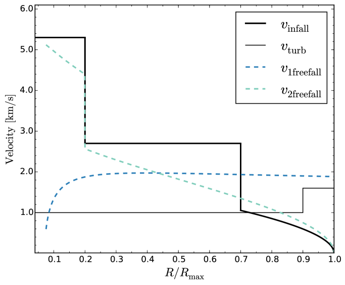
Figure 13: Resulting velocity, $\varv_{\rm infall}$, and turbulent profile, $\varv_{\rm turb}$, as a function of the normalized radius of the cloud, obtained for the best-fitting ALI model (black solid lines). Velocity profile obtained for free-fall when modeling with one component (see Fig. 17), $\varv_{\rm 1freefall}$ (blue dashed line), and two components (see Fig. 15), $\varv_{\rm 2freefall}$ (green dashed line).

The best-fit model has both turbulence and infall that vary with radius (see Fig. 13). Analysis of the absorbing material towards G34 suggests a scenario where two and possibly a third gas envelope are moving inwards toward the central region, where the two inner ones have constant velocities and the third outermost envelope (where r ¿ 0.7 R_max) has a free-fall velocity profile.

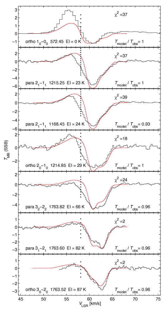
Figure 14: ALI: Two velocity regimes with constant profiles using 5.3 km s^-1 in the inner and 2.7 km s^-1 in the outer region. $\sum{\chi^{2}_{\rm line}}$ = 121 , over $\Delta V_{\mathrm{LSR}}=54-68$ km s^-1. Notation as in Fig. 10.

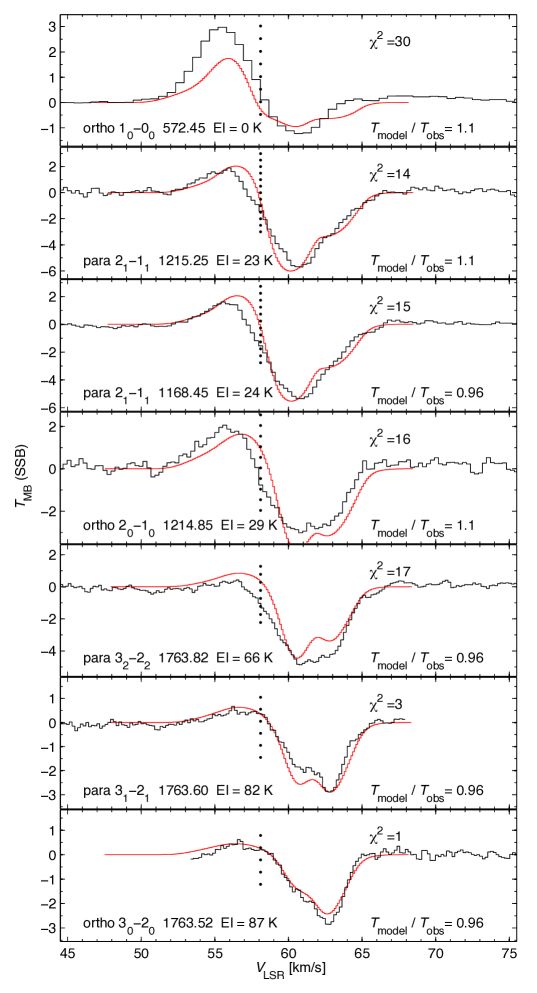
Figure 15: ALI: Two velocity regimes with free-fall using $f$ = 0.7 in the inner and $f$ = 0.4 in the outer region, $M_{0}=400$ M_⊙ and $a$ = 1. Notation as in Fig. 10. $\sum{\chi^{2}_{\rm line}}$ = 65.

In order to produce an acceptable fit at least two velocity regimes are needed. Either two constant velocity regimes, with infall at 5.3 km s^-1 for r ¡ 0.2 and 2.7 km s^-1 for r ¿ 0.2, shown in Fig. 14, or two in free-fall, shown in Fig. 15 (see velocity profile shown in Fig. 13). The former models the absorption profiles well, especially at higher velocities. The latter models the emission and absorption at lower velocities better, and require free-fall velocity fractions of $f$ = 0.7 and 0.4 for the inner and outer velocity field respectively. In addition, it needs the mass contained in the compact central object (within radius $R_{\rm ph}$) to be on the order of $\sim$400 $M_{\odot}$.

Thus, a combination of these two models produces the best-fit as shown in Fig. 10. If the mass of the central source, $M_{0}$, is taken to be less than 300 M_⊙ it will not affect the free-fall velocity ($\varv_{\rm infall}$) profile in the outer envelope, and a higher mass will shift the absorption minima to higher velocities and increase the sum of $\chi^{2}_{\rm line}$. Therefore, $M_{0}$ is set to be equal to 1 M_⊙.

Micro turbulence

The ”two-step profile” for the turbulence (see Table LABEL:Table:model for details) provided better fits for all the line profiles, compared with setting the micro turbulence as constant through the source. Thus we adopted an increase of the micro turbulence from unity to 1.6 km s^-1 in the outer envelope (cf. Liu et al., 2013; Herpin et al., 2012; Caselli & Myers, 1995). This parameter adjusts the detailed profile shapes.

6.2 Modeling

The first step of modeling the seven ammonia transitions in ALI was to adopt the parameters used by Wyrowski et al. (2012) to model the infalling component at about 61 km s^-1 observed in the $3_{2,-}-2_{2,-}$ NH₃ transition at 1810 GHz (see Fig.3), obtained by SOFIA. Its critical density is similar to those of the 1764 GHz transitions and therefore might share the same environmental origin. We implemented the same temperature and density profile as given in Rolffs et al. (2011) and a free-fall velocity field as given in Wyrowski et al. (2012), where fff = 0.3, $M_{0}=20$ M_⊙ and $a$ = 1000. While the 61 km s^-1 absorption of the 1764 GHz line could be reasonably fit, the model overestimates the blue-shifted emission and cannot reproduce the red-shifted absorption component at 63 km s^-1. This led us to the changes in the physical structure discussed in Sect. 6 which resulted in our best-fit model.

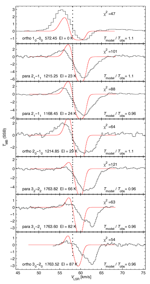
Figure 17: ALI: One velocity regime with free-fall using $f$ = 0.3, $M_{0}=20$ M_⊙ and $a$ = 1000. Notation as in Fig. 10. $\sum{\chi^{2}_{\rm line}}$ = 491.

Using the best-fit density profile (see Sect. 6) when adopting the one component free-fall velocity, the infalling component at about 61 km s^-1 is poorly modeled. See velocity profile, $\varv_{\rm 1freefall}$, shown in Fig. 13 and modeled line profiles shown in Fig. 17.

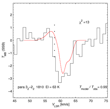
Figure 18: ALI: Best-fit model applied on the 1810 GHz transition and multiplied by a factor of 30% to reproduce the continuum. Notation as in Fig. 10.

The best-fit model also reproduces well the profile of the 1810 GHz transition (Fig.18). In fact, the fit is somewhat better than for the corresponding Herschel-HIFI transition at 1763.8 GHz (i.e., $\sum{\chi^{2}_{\rm line}}$ = 13 vs 20). The 30% discrepancy in continuum flux could well be within the calibration uncertainty of that observation.

The infalling component at about 61 km s^-1 was modeled by Wyrowski et al. (2012) for NH₃ but also by Coutens et al. (2014) for HDO. At a corresponding radius of r = 0.066 $R_{\rm max}$ in the best-fit model, Coutens et al. (2014) modeled an expanding region set to 4 km s^-1. When this velocity is applied to the best-fit model at r ¡ 0.075, the absorption components are not affected, but the peak of the emissions is narrower. Still, it does not produce a lower $\sum{\chi^{2}_{\rm line}}$ value than the best-fit model. As a result, we can neither confirm nor refute the presence of an expansion in the inner parts of the envelope.

7 The mass accretion process

The very first stage of the formation of massive OB stars is believed to be initiated by contraction and fragmentation of dense molecular cores in approximate hydrostatic equilibrium (Garay & Lizano, 1999). The question is then how a molecular core evolves to produce one or several massive stars? High amounts of mass must be able to feed the star on short time-scales despite the strong radiation pressure. Models have shown that transfer of matter through a protostar-disk system is very efficient in order to accrete matter to the star (see Sect. 1)

Accretion can proceed if its rate is higher than the mass that can be supported by radiation pressure from the luminous protostars. Our highly resolved multitransition study confirms the inward motion shown by Wyrowski et al. 2012, but it also shows increased velocity with increased excitation. With a spherically symmetric accreting envelope, the best-fit model can reproduce the line profiles and continuum. The size of the accreting envelope is clearly larger than the separations of MYSOs in the embedded cluster. The mass in each shell of the envelope of our model can be interpreted as separate, each moving inwards. This result is consistent with the competitive accretion model (Bonnell et al., 1997, 2001), in which many YSO compete for the same reservoir of material.

The mass accretion rate at any radius $R$ can be estimated by means of the method of Beltrán et al. (2006)

$$\dot{M}_{\rm acc}=4\pi\,R^{2}\,m_{\rm H_{2}}\,n_{\rm H_{2}}\,\varv_{\rm infall},$$ (6)

where $m_{\rm H_{2}}$ is the mass of the H₂ molecule, $n_{\rm H_{2}}$ is the gas volume density of molecular hydrogen, and $\varv_{\rm infall}$ is the infall velocity as a function of the radius $R$ as described in Table. LABEL:Table:model.

The inferred mass accretion rate starts from zero at $R_{\rm max}$ and increases inwards together with the free infall velocity and the $n_{\rm H_{2}}$. When the velocity in the outer envelope is free-falling the mass accretion rate ($4.5\times 10^{-3}$ M_⊙yr^-1) supports estimates made by Wyrowski et al. (2012), Klaassen & Wilson (2007) and Liu et al. (2013). As the velocity jumps up to 2.7 km s^-1, at r = 0.7$R_{\rm max}$, the mass accretion rate also jumps up to $1.2\times 10^{-2}$ M_⊙yr^-1. Within the inner 20% of the envelope, where the infall velocity is 5.3 km s^-1, $\dot{M}_{\rm acc}$ increases to $3.0\times 10^{-2}$ M_⊙yr^-1. At 0.075$R_{\rm max}$, where the number density and velocity are the highest, the mass accretion rate reaches its maximum and is $4.5\times 10^{-2}$ M_⊙yr^-1, just before the profile of $n_{\rm H_{2}}$ decreases to $2.3\times 10^{6}$ cm^-3. The apparent decrease in mass-accretion rate at r ¡ 0.075 $R_{\rm max}$, where the gas density has been artificially truncated, signifies that the accretion must shut off at the surface of the IR-continuum object. The resulting profile of the mass accretion rate is shown in Fig. 12.

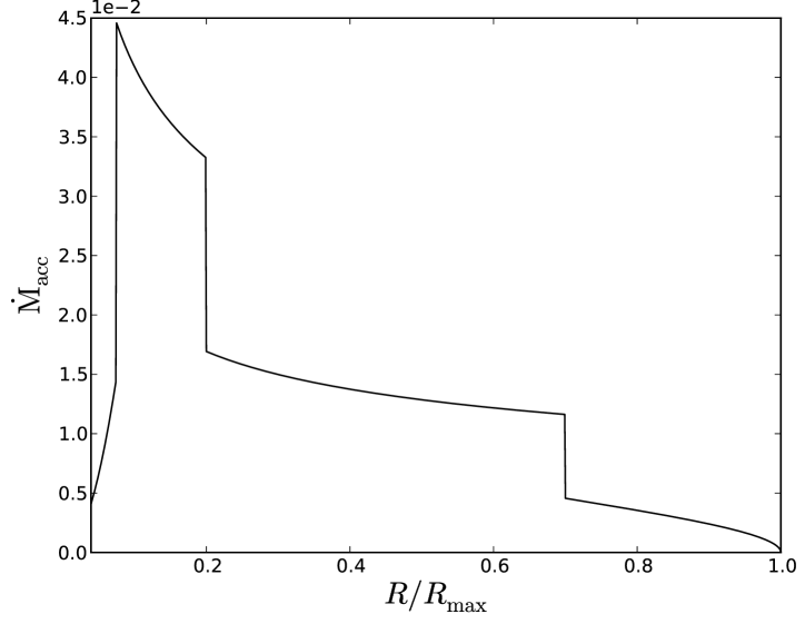
Figure 12: Resulting mass accretion profile, $\dot{M}_{\rm acc}$ [ M_⊙yr^-1], obtained in the best-fit ALI model as a function of the normalized radius of the cloud.

We speculate that the modeled flat inner density profile may originate from an accretion disk, which is fed by the infalling envelope. This is also supported by observations made by Keto et al. (1987b) of G34 that suggest high rotational velocities. From the radial size of the inner constant density profile the accretion disk is about 9000 AU in radius, which could mean that the possible accretion disk is large enough to enclose several protostars. Protostars surrounded by an accretion disk, with an ensemble of molecular clumps falling inwards, agrees well with the dynamical competitive accretion model.

The overall high infall velocities through the envelope and the high mass infall rates for G34 are expected for more evolved MSF regions compared with the stages prior to the hot core phase (Liu et al., 2013). The mass accretion rates are high enough (¿$10^{-3}$ M_⊙yr^-1) throughout the envelope to quench the H II region in G34 (Walmsley, 1995; Wolfire & Cassinelli, 1987) and to overcome the radiation pressure from the forming (proto) cluster.

If there existed an outward motion in the innermost region, as suggested by Coutens et al. (2014), then the mass accretion rate would be zero in this region. Non-spherical symmetric motions of gas and dust would be needed to feed the protostars in the cluster, which is consistent with the competitive accretion model.

We stress that the derived high mass accretion rates assume spherically symmetric accretion, which may not be true. The true accretion rate could be different if the accretion is non-uniform or lacks spherical symmetry. If this is the case, the minimum fraction of the spherically symmetric mass accretion rate needed for the shell to be able to quench the H II region at radius, $R_{\rm ph}$, $0.075R_{\rm max}$, $0.2R_{\rm max}$ and 0.7$R_{\rm max}$, are: 24%, 2.2%, 3.3%, 22%, respectively. However, it is beyond the scope of this paper to consider the different distribution of radiation pressure on the accreting clumps compared to the case of spherically symmetric accretion.

The central mass of the source has a great influence on the free-fall velocity field(s), thus the mass accretion rate. From literature, the masses estimated from high-resolution observations of the central core of G34 are 76 to 360 M_⊙ (Liu et al., 2013; Watt & Mundy, 1999; Garay et al., 1986). The observed core has a diameter of $2\times R_{\rm ph}$ that spans about 1.4 ″on the sky at 3.3 kpc distance. This is in agreement of the upper limit of approximately 300 M_⊙ in the central source found in our best-fit model.

7.1 Modeling limitations

Since our model is based on spherical symmetry it has limited abilities to take into account clumpy distributions of gas and dust and asymmetric outflow. The compact H II region in G34 is far from spherically symmetric since component C has a cometary tail on large scales (see Fig. 1) where most likely the bulk of the emission and absorption of the 572 GHz line is produced. The shape makes the density distribution non-symmetric, having lower density to the right part of the tail compared to the left side. The influence of these components may result in an underestimation of the absorption. The resulting line profile is also affected by surrounding molecules, which is beyond the scope of our model. The broad redshifted emission of o-NH₃ (572 GHz) and o-H₂O (557 GHz) trace a broad outflow component, estimated to be large enough to support the scale of a molecular champagne flow as a result of the evolved H II region, expanding as a bubble until it reaches less dense ISM and breaks. The morphology, age and driving source of the subparsec-scale outflow components (see Sect. 1, Imai et al., 2011; Klaassen & Wilson, 2007) are still unknown but have suggested to be associated with individual YSO harboring a turbulent disk (Heaton et al., 1985), as observed in low-mass objects. They should give rise to bipolar collimated outflows, however the reason why we are only detecting the red-shifted part must be that the the opposite outflow lobe is directed tangentially to our line of sight and therefore is invisible to the telescope.

The high luminosity of G34 implies that massive (proto)stars are the heating engine, although we have modeled the source with only one central heating source. Multiplicity could indeed partly explain the deviations between model and data, since the sources are clustered from the onset. A more realistic picture of a forming star cluster would include multiple heating sources, which is impossible for our model to cover.

Limited computational power prevented tests of all model combinations and allowed only a simple chemical structure, not computed from chemical models. The gas-to-dust mass ratio, emissivity parameter and the dust frequency dependence are assumed to be constant throughout the source, although they are likely to vary (e.g., due to evaporation of ice mantles).

8 Conclusions

In this paper we have presented seven velocity-resolved rotational lines of ammonia toward the ultra compact HII region G34.26+0.15. The mixed absorption and emission in the line profiles was successfully modeled with the radiative transfer code ALI (see Fig. 10).

The narrow-emission part of all the seven ammonia line profiles and the absorption for the ground-state line, are quite well reproduced, except for the emission part for a few transitions. This can be the result of assuming that the enveloping matter is spherically symmetric. We also found that the one-jump velocity and density models have a great influence on the NH₃ line profiles. To allow probing of the hot core, observations of higher-energy ammonia transitions are needed for opacity reasons. The fundamental 1₀–0₀ ortho transition 572 GHz shows a possible molecular outflow activity that probably is caused by bipolar outflows, but to rule out a champagne outflow is beyond the scope of this paper.

We derived ammonia abundances relative to molecular hydrogen in the inner, middle and outer region of the envelope to be $X_{\rm in}=1.8\times 10^{-9}$, $X_{\rm mid}=1.2\times 10^{-9}$ and $X_{\rm out}=3.0\times 10^{-9}$, respectively. The overall low derived abundances suggest that the molecular gas is not yet in steady-state. Alternatively, our assumption of equal gas and dust temperatures might break down in the low-density region. The enriched abundance in the outer region is most likely because of UV photo-desorption. In the inner region, the high temperature will partially release NH₃ from the water ice matrix on dust particles and increase the ammonia abundance. From modeling we derived an ammonia OPR of $\sim$ 0.5, in agreement with recent findings in translucent interstellar gas (Persson et al., 2012).

Our derived accretion rates are found to be $0.41-4.5\times 10^{-2}$ [M_⊙ yr^-1], which is high enough to overcome the radiation pressure from G34. Even though the observed transitions only probe the dynamics of the envelope and the outer parts of the hot core, the mass accretion profile shown in Fig. 12 may, however, indicate that the accretion already has halted in the inner part of the hot core. We speculate that this may be due to an outflow activity or an accretion disk, alternatively that we no longer can use ammonia to trace the mass close to the central source as it will be ionized/dissociated.

Our results demonstrate that rotational transitions of ammonia seen in absorption toward a strong far-infrared continuum source can successfully be used to probe infall velocities, physical and chemical properties in a variety of evolutionary stages of MSF cloud cores.

Appendix A Online Material: Details of the observations and examples of less successful models.

Table 5: G34.26+0.15: $Herschel$-HIFI OBSID’s of the observed transitions analysed in this paper.

Specie	Frequency	Band	LO-setting	Date	OBSID
	(GHz)
o-$\@element[3]{\mathrm{NH}}$	572.498	1b (USB)	A	2011-04-22	1342219281
			B		1342219282
			C		1342219283
	1214.852	5a (USB)	A	2011-03-13	1342215886
			B		1342215884
			C		1342215885
	1763.524	7a (USB)	A	2012-04-20	1342244604
			B		1342244605
			C		1342244606
p-$\@element[3]{\mathrm{NH}}$	1215.245	5a (USB)	A	2011-04-22	1342215886
			B		1342215884
			C		1342215885
	1168.454	5a (LSB)	A	2012-04-18	1342244518
			B		1342244517
			C		1342244519
	1763.824	7a (USB)	A	2011-04-20	1342244604
			B		1342244605
			C		1342244606
	1763.602	7a (USB)	A	2011-04-20	1342244604
			B		1342244605
			C		1342244606