Runge-Kutta time semidiscretizations of semilinear PDEs with non-smooth data

Abstract.

We study semilinear evolution equations $\frac{\mathrm{d}U}{\mathrm{d}t}=AU+B(U)$ posed on a Hilbert space $\mathcal{Y}$, where $A$ is normal and generates a strongly continuous semigroup, $B$ is a smooth nonlinearity from $\mathcal{Y}_{\ell}=D(A^{\ell})$ to itself, and $\ell\in I\subseteq[0,L]$, $L\geq 0$, $0,L\in I$. In particular the one-dimensional semilinear wave equation and nonlinear Schrödinger equation with periodic, Neumann and Dirichlet boundary conditions fit into this framework. We discretize the evolution equation with an A-stable Runge-Kutta method in time, retaining continuous space, and prove convergence of order $O(h^{p\ell/(p+1)})$ for non-smooth initial data $U^{0}\in\mathcal{Y}_{\ell}$, where $\ell\leq p+1$, for a method of classical order $p$, extending a result by Brenner and Thomée for linear systems. Our approach is to project the semiflow and numerical method to spectral Galerkin approximations, and to balance the projection error with the error of the time discretization of the projected system. Numerical experiments suggest that our estimates are sharp.

Keywords: Semilinear evolution equations, $A$-stable Runge Kutta semidiscretizations in time, fractional order of convergence.
AMS subject classification: 65J08, 65J15, 65M12, 65M15.

1. Introduction

We study the convergence of a class of A-stable Runge-Kutta time semidiscretizations of the semilinear evolution equation

$$\frac{\mathrm{d}U}{\mathrm{d}t}=AU+B(U)$$ (1.1)

for non-smooth initial data $U(0)=U^{0}$. In the examples we have in mind (1.1) is a partial differential equation (PDE). We assume that (1.1) is posed on a Hilbert space $\mathcal{Y}$, $A$ is a normal linear operator that generates a strongly continuous semigroup, and that $B$ is smooth on a scale of Hilbert spaces $\{\mathcal{Y}_{\ell}\}_{\ell\in I}$, $I\subseteq[0,L]$, $0,L\in I$, as detailed in condition (B) below. Here $\mathcal{Y}_{\ell}=D(A^{\ell})\subseteq\mathcal{Y}$, $\ell\geq 0$. Note that condition (B) depends on both, the smoothness properties of the nonlinearity $B(U)$ and the boundary conditions. Under these assumptions the class of equations we consider includes the semilinear wave equation and the nonlinear Schrödinger equation in one spatial dimension with periodic, Neumann and Dirichlet boundary conditions (see Examples 2.3 - 2.8 below). For an example in three space dimensions see Example 5.4. We discretize (1.1) in time by an $A$-stable Runge Kutta method; the condition of $A$-stability ensures that the numerical method is well-defined on $\mathcal{Y}$, and is satisfied by a large class of methods including the Gauss-Legendre collocation methods.

Discretizing in time while retaining a continuous spatial parameter means that we consider the numerical method as a nonlinear operator on the infinite dimensional space $\mathcal{Y}$. This leads to several technicalities, in particular existence results for the numerical method $\Psi^{h}$ as well as the semiflow $\Phi^{t}$ and regularity of solutions in both cases are required to ensure convergence results analogous to the finite dimensional case. In [15], existence and regularity of the semiflow of (1.1) on a scale of Hilbert spaces, corresponding results for the numerical method, and full order convergence of the time semidiscretization for sufficiently smooth data are studied in detail. We review the relevant results in Sections 2 and 3.

In this paper we consider the effect of non-smooth data on the order of convergence of the time semidiscretization in this setting. We consider an $A$-stable Runge-Kutta method of classical order $p$ applied to the problem (1.1) with initial data $U^{0}\in\mathcal{Y}_{\ell}$, $\ell\in I$. The main result we give here, Theorem 5.3, shows that we can expect order of convergence $\mathcal{O}(h^{q})$ where $q(\ell)=p\ell/(p+1)$ for $0\leq\ell<p+1$. This corresponds closely with numerical observation, cf. Figure 1. Given a time $T>0$ we prove the above order of convergence for the time-semidiscretization up to time $T$ for any solution $U(t)$ of (1.1) with a given $\mathcal{Y}_{\ell}$ bound. Here $\ell>0$ is such that $\ell-k\in I$ for $k=1,\ldots,\lfloor\ell\rfloor$ (the greatest integer $\leq\ell$). It is shown in [15] that for $\ell\geq p+1$ we have full order of convergence $\mathcal{O}(h^{p})$.

The reduction in order of the method from $p$ to $q$ for $\ell<p+1$ is caused by the occurrence of unbounded operators in the Taylor expansion of the one-step error coefficient. Our approach is to apply a spectral Galerkin approximation to the semiflow of the evolution equation (1.1), and to discretize the projected evolution equation in time. This allows us to bound the size of the local error coefficients in terms of the accuracy of the projection. By balancing the projection error with the growth of the local error coefficients we obtain the estimates of our main result, Theorem 5.3.

Related results include those of Brenner and Thomée [3], who consider linear evolution equations $\dot{U}=AU$ in a more general setting, namely posed on a Banach space $\mathcal{X}$, where $A$ generates a strongly continuous semigroup $e^{tA}$ on $\mathcal{X}$. They show $O(h^{q})$ convergence of A-acceptable rational approximations of the semigroup for non-smooth initial data $U^{0}\in D(A^{\ell})$, $\ell=0,\ldots,p+1$, with $q=q(\ell)=p\ell/(p+1)$ as above, if $\ell>(p+1)/2$ (when $\ell\leq(p+1)/2$ they prove convergence with order $q(\ell)<p\ell/(p+1)$). Kovács [9] generalizes this result to certain intermediate spaces with arbitrary $\ell\in[0,p+1]$ and also provides sufficient conditions for when $q=q(\ell)=p\ell/(p+1)$ for all $\ell\in[0,p+1]$ (which are satisfied in our setting).

For splitting methods, where the linear part of the evolution equation is evaluated exactly, a higher order of convergence has been obtained for specific choices of $\ell$ and specific evolution equations in [13] and [6], see also Example 5.4 below. While splitting methods are very effective for simulating evolution equations for which the linear evolution $\mathrm{e}^{tA}$ can easily be computed explicitly, Runge–Kutta methods are still a good choice when an eigen-decomposition of $A$ is not available, for example for the semilinear wave equation in an inhomogeneous medium, see Example  2.7. Moreover, the simplest example of a Gauss–Legendre Runge-Kutta method, the implicit mid point rule, appears to have some advantage over split step time-semidiscretizations for the computation of wave trains for nonlinear Schrödinger equations because the latter introduce an artificial instability [18].

For Runge-Kutta time semidiscretizations of dissipative evolution equations, where $A$ is sectorial, a better order of convergence can be obtained, see [10] for the linear case and [11, 12] and references therein for the semilinear case. Note that our approach is different from the approach of [11, 12]. In [11, 12] some smoothness of the continuous solution is assumed and from that a (fractional) order of convergence is obtained, using the variation of constants formula. The order of convergence obtained in [11, 12] is in general lower than in the linear case (where full order of convergence is obtained in the parabolic case [10]), but no extra assumptions on the nonlinearity $B(U)$ of the PDE are made. In particular in [12, Theorems 4.1 and 4.2] the existence of $(p_{s}+2)$ time derivatives of the continuous solution $U(t)$ of a semilinear parabolic PDE (1.1) is assumed, where $p_{s}$ is the stage order of the method. This assumption is then used to estimate the error of the numerical approximation of the inhomogenous part of the variation of constants formula. Here the stage order $p_{s}$ comes into play. Note that if the nonlinearity $B(U)$ of the evolution equation (1.1) only satisfies the standard assumption rather than our assumption (B), i.e., is smooth on $\mathcal{Y}$ only (so that the Hilbert space scale is trivial with $L=0$) then the existence of $U^{\prime}(t)$ can be guaranteed for $U^{0}\in\mathcal{Y}_{1}$ by semigroup theory [17], but it is not clear whether higher order time derivatives of the solution $U(t)$ of (1.1) exist as assumed in [12] - therefore in [12] also time-dependent perturbations of (1.1) are considered. In this paper we instead take the approach of making assumptions (namely condition (B) on the nonlinearity $B(U)$ of the evolution equation and the condition that $U^{0}\in\mathcal{Y}_{\ell}$) which are straightforward to check and guarantee the existence of the time derivatives of the continuous solution $U(t)$ up to order $k\leq\ell$. We then obtain an order of convergence $O(h^{p\ell/(p+1)})$ of the Runge-Kutta discretization which is identical to the order of convergence in the linear case [3, 9]. In [11, Theorem 2.1] some smoothness of the inhomogeneity of the PDE is obtained from the smoothing properties of parabolic PDEs, and this is used to prove an order of convergence $h\log h$, without the assumption of the existence of higher time derivatives of the continuous solution $U(t)$. Here we do not consider parabolic PDEs, so that we cannot use this strategy.

Alonso-Mallo and Palencia [2] study Runge-Kutta time discretizations of inhomogeneous linear evolution equations where the linear part creates a strongly continuous semigroup. Similarly as in [12] they obtain an order of convergence depending on the stage order $p_{s}$ of the Runge-Kutta method. They assume the continuous solution $U(t)$ to be $(p+1)$-times differentiable in $t$, but in their context the condition $U(t)\in D(A^{p-p_{s}})$, where $p$ is the order of the numerical method, is in general not satisfied due to the inhomogeneous terms in the evolution equation, and this leads to a loss in the order of convergence compared to our results. Note that in our setting, due to our condition (B) on the nonlinearity, provided $U(0)\in\mathcal{Y}_{p+1}$ we have $U(t)\in D(A^{p+1})=\mathcal{Y}_{p+1}$ and $U(t)$ is $p+1$ times differentiable in $t$ (in the $\mathcal{Y}$ norm) and so we get full order of convergence in this case (see [15]). Calvo et al [4] study Runge-Kutta quadrature methods for linear evolution equations $\dot{U}(t)=A(t)U(t)$ which are well-posed and prove full order convergence if the continuous solution $U(t)$ has $p+1$ time derivatives; they also obtain fractional orders of convergence as in [3] for solutions $U(t)\in\mathcal{Y}_{\ell}$ with $\ell<p+1$.

We proceed as follows: in Section 2 we introduce the class of semilinear evolution equations that we consider in this paper, give some examples, review existence and regularity results of [17, 15] for the semiflow, and adapt them to the case of non-integer $\ell$. In Section 3 we introduce a class of $A$-stable Runge-Kutta methods. We review existence and regularity of these methods when applied to the semilinear evolution equation (1.1) and a convergence result for sufficiently smooth initial data from [15]. In Section 4 we study the stability of the semiflow and numerical method under spectral Galerkin truncation, and establish estimates for the projection error. Lemma 4.2 and 4.3 are established in [16] for integer values of $\ell$; for completeness we review the proofs, which also work for non-integer $\ell$. In Section 5 we prove our main result on convergence of $A$-stable Runge-Kutta discretizations of semilinear evolution equations for non-smooth initial data. In Section 6 we generalize our result to nonlinearities $B(U)$ which are defined on domains other than balls.

2. Semilinear PDEs on a scale of Hilbert spaces

In this section we introduce a suitable functional setting for the class of equations we subsequently study. We review results from [17, 15] on the local well-posedness and regularity of solutions of (1.1) and give examples.

For a Hilbert space $\mathcal{X}$ we let

$$\mathcal{B}^{R}_{\mathcal{X}}(U^{0})=\{U\in\mathcal{X}:\lVert U-U^{0}\rVert_{\mathcal{X}}^{\vphantom{1}}\leq R\}$$

be the closed ball of radius $R$ around $U^{0}$ in $\mathcal{X}$. We make the following assumptions on the semilinear evolution equation (1.1):

1. $A$ is a normal linear operator on $\mathcal{Y}$ that generates a strongly continuous semigroup of linear operators $e^{tA}$ on $\mathcal{Y}$ in the sense of [17].

It follows from assumption (A) that there exists $\omega\in\mathbb{R}$ with

$$\mathfrak{Re}(\operatorname{spec}(A))\leq\omega,\quad\lVert e^{tA}\rVert_{\mathcal{Y}\to\mathcal{Y}}^{\vphantom{1}}\leq e^{\omega t},$$ (2.1)

see [17]. In light of (A) we define the continuous scale of Hilbert spaces $\mathcal{Y}_{\ell}=D(A^{\ell})$, $\ell\geq 0$, $\mathcal{Y}_{0}=\mathcal{Y}$. Thus the parameter $\ell$ is our measure of smoothness of the data. For $m>0$ we define $\mathbb{P}_{m}$ to be the spectral projection of $A$ to $\operatorname{spec}(A)\cap\mathcal{B}^{m}_{\mathbb{C}}(0)$, let $\mathbb{Q}_{m}=\operatorname{id}-\mathbb{P}_{m}$ and set $\mathbb{P}=\mathbb{P}_{1}$, $\mathbb{Q}=\operatorname{id}-\mathbb{P}$. We endow $\mathcal{Y}_{\ell}$ with the inner product

$$\langle U_{1},U_{2}\rangle_{\mathcal{Y}_{\ell}}^{\vphantom{1}}=\langle\mathbb{P}U_{1},\mathbb{P}U_{2}\rangle_{\mathcal{Y}}^{\vphantom{1}}+\langle|A|^{\ell}\mathbb{Q}U_{1},|A|^{\ell}\mathbb{Q}U_{2}\rangle_{\mathcal{Y}}^{\vphantom{1}},$$ (2.2)

which implies

$$\|A^{\ell}\|_{\mathcal{Y}_{\ell}\to\mathcal{Y}}\leq 1.$$ (2.3)

We deduce from assumption (A) that for $u\in\mathcal{Y}$, $\lim_{m\to\infty}\mathbb{P}_{m}u=u$, and from (2.2) the estimates

$$\lVert A^{\ell}\mathbb{P}_{m}U\rVert_{\mathcal{Y}}^{\vphantom{1}}\leq m^{\ell}\lVert\mathbb{P}_{m}U\rVert_{\mathcal{Y}}^{\vphantom{1}},\quad\|\mathbb{P}_{m}\|_{\mathcal{Y}_{\ell}\to\mathcal{Y}_{\ell+k}}\leq m^{k},\quad\lVert\mathbb{Q}_{m}U\rVert_{\mathcal{Y}}^{\vphantom{1}}\leq m^{-\ell}\lVert U\rVert_{\mathcal{Y}_{\ell}}^{\vphantom{1}}$$ (2.4)

for $\ell\geq 0$, $k\geq 0$, $m\geq 1$.

Remark 2.1.

When $\ell$ lies in a discrete set such as $\mathbb{N}_{0}$, for $\ell>0$ often the inner product

$$\langle U_{1},U_{2}\rangle_{\ell}^{\vphantom{1}}=\langle U_{1},U_{2}\rangle_{\mathcal{Y}}^{\vphantom{1}}+\langle A^{\ell}U_{1},A^{\ell}U_{2}\rangle_{\mathcal{Y}}^{\vphantom{1}}$$ (2.5)

is used on $\mathcal{Y}_{\ell}$ instead of (2.2). For $\ell=0$, for consistency, one defines $\langle U_{1},U_{2}\rangle_{0}^{\vphantom{1}}=\langle U_{1},U_{2}\rangle_{\mathcal{Y}}^{\vphantom{1}}$. The reason why we do not use this inner product here is that (2.2) is continuous in $\ell$ as $\ell\to 0$, but the graph inner product (2.5) is not: we have $\lim_{\ell\to 0}\langle U_{1},U_{2}\rangle_{\ell}^{\vphantom{1}}=2\langle U_{1},U_{2}\rangle_{\mathcal{Y}}^{\vphantom{1}}=2\langle U_{1},U_{2}\rangle_{0}^{\vphantom{1}}$.

To formulate our second assumption, on the nonlinearity $B$, we introduce the following notation: for Banach spaces $\mathcal{X}$, $\mathcal{Z}$, we denote by $\mathcal{E}^{i}(\mathcal{X},\mathcal{Z})$ the space of $i$-multilinear bounded mappings from $\mathcal{X}$ to $\mathcal{Z}$. For $\mathcal{U}\subseteq\mathcal{X}$ we write $\mathcal{C}_{\operatorname{b}}^{k}(\mathcal{U},\mathcal{Z})$ to denote the set of $k$ times continuously differentiable functions $F\colon\operatorname{int}\mathcal{U}\to\mathcal{Z}$ such that $F$ and its derivatives $\mathrm{D}^{i}F$ are bounded as maps from the interior $\operatorname{int}\mathcal{U}$ of $\mathcal{U}$ to $\mathcal{E}^{i}(\mathcal{X},\mathcal{Z})$ and extend continuously to the boundary of $\operatorname{int}\mathcal{U}$ for $i\leq k$. We set $\mathcal{C}_{\operatorname{b}}(\mathcal{U},\mathcal{Z})=\mathcal{C}_{\operatorname{b}}^{0}(\mathcal{U},\mathcal{Z})$. Note that if $\dim\mathcal{X}=\infty$, there are examples of continuous functions $F:\mathcal{U}\to\mathcal{Z}$ where $\mathcal{U}$ is closed and bounded, which do not lie in $\mathcal{C}_{\operatorname{b}}(\mathcal{U},\mathcal{Z})$, see e.g. [15, Remark 2.3]. In the following for $\ell\in\mathbb{R}$ let $\lfloor\ell\rfloor$ be the largest integer less than or equal to $\ell$ and $\lceil\ell\rceil$ be the smallest integer greater or equal to $\ell$. Moreover for $R>0$ and $\ell\geq 0$ we abbreviate

$$\mathcal{B}_{\ell}^{R}=\mathcal{B}_{\mathcal{Y}_{\ell}}^{R}(0).$$ (2.6)

We are now ready to formulate our condition on the nonlinearity $B(U)$ of (1.1).

1. There exists $L\geq 0$, $I\subseteq[0,L]$, $0,L\in I$, $N\in\mathbb{N}$, $N>\lceil L\rceil$, such that $B\in\mathcal{C}_{\operatorname{b}}^{N-\lceil\ell\rceil}(\mathcal{B}^{R}_{\ell};\mathcal{Y}_{\ell})$ for all $\ell\in I$ and $R>0$.

We denote the supremum of $B:\mathcal{B}_{\ell}^{R}\to\mathcal{Y}_{\ell}$ as $M_{\ell}[R]$ and the supremum of its derivative as $M^{\prime}_{\ell}[R]$, and set $M[R]=M_{0}[R]$ and $M^{\prime}[R]=M^{\prime}_{0}[R]$. Moreover we define

$$I^{-}:=\{\ell\in I,\ell-k\in I,k=1,\ldots,\lfloor\ell\rfloor\}.$$ (2.7)

We seek a solution $U(\cdot)\in\mathcal{C}([0,T];\mathcal{Y}_{\ell})$ of (1.1) for some $T>0$, $\ell\in I$, with initial data $U(0)=U^{0}\in\mathcal{Y}_{\ell}$, and write $\Phi^{t}(U^{0})\equiv\Phi(U^{0},t)\equiv U(t)$. The following result is an extension of Theorem 2.4 of [15], see also [17], to non-integer $\ell$ and provides well-posedness and regularity of the semiflow $\Phi^{t}$ under suitable assumptions.

Theorem 2.2 (Regularity of the semiflow).

Assume that the semilinear evolution equation (1.1) satisfies (A) and (B). Let $R>0$. Then there is $T_{*}>0$ such that there exists a semiflow $\Phi$ which satisfies

$$\Phi^{t}\in\mathcal{C}_{\operatorname{b}}^{N}(\mathcal{B}_{0}^{R/2};\mathcal{B}^{R}_{0})$$ (2.8a)

with uniform bounds in $$t\in[0,T_{*}] \ell\in I^{-} k\in\mathbb{N}_{0} k\leq\ell$$. Moreover if and satisfies , then

$$\Phi(U)\in\mathcal{C}_{\operatorname{b}}^{k}([0,T_{*}];\mathcal{B}^{R}_{0})$$ (2.8b)

with uniform bounds in $$U\in\mathcal{B}_{\ell}^{R/2}$$.

The bounds on $T_{*}$ and $\Phi$ depend only on $R$, $\omega$ from (2.1), and the bounds afforded by assumption (B) on balls of radius $R$.

Proof.

The proof of (2.8b) is an application of a contraction mapping theorem with parameters to the map

$$\Pi(W,U,T)=e^{tTA}U+\int_{0}^{t}e^{T(t-\tau)A}B(W(\tau))\mathrm{d}\tau,$$ (2.9)

on the scale of Banach spaces $\mathcal{Z}_{\ell}=\mathcal{C}_{\operatorname{b}}([0,1];\mathcal{Y}_{\ell})$, $\ell\in I$, where we define $\mathcal{Z}:=\mathcal{Z}_{0}$. The solution $W(U,T)(t)=\Phi^{tT}(U)$ of (1.1) is obtained as a fixed point of (2.9) for $U\in\mathcal{B}^{R/2}_{\mathcal{Y}}(0)$ as in [15]. Here $\Pi:\mathcal{B}^{R}_{\mathcal{Z}}(0)\times\mathcal{B}^{R/2}_{\mathcal{Y}}(0)\times[0,T_{*}]\to\mathcal{Z}$. In order to apply the contraction mapping theorem we first check that $\Pi(W,\cdot,\cdot)$ maps $\mathcal{B}^{R}_{\mathcal{Z}}(0)$ to itself: For $U\in\mathcal{B}^{R/2}_{\mathcal{Y}}(0)$ we have

$$\|\Pi(W,U,T)\|_{\mathcal{Z}} \leq\max_{\tau\in[0,1]}\|\mathrm{e}^{\tau TA}U\|_{\mathcal{Y}}+T\mathrm{e}^{\omega T}M_{0}[R]$$ (2.10)

$$\leq\mathrm{e}^{\omega T}R/2+T\mathrm{e}^{\omega T}M_{0}[R]\leq R$$

for $T\in[0,T_{*}]$ and $T_{*}$ small enough. So $\Pi$ maps $\mathcal{B}^{R}_{\mathcal{Z}}(0)$ to itself. Moreover for sufficiently small $T_{*}$ there is $c\in[0,1)$ such that $\|\mathrm{D}\Pi(W,U,T)\|_{\mathcal{Z}\to\mathcal{Z}}\leq c$ for all $W\in\mathcal{B}^{R}_{\mathcal{Z}}(0)$, $U\in\mathcal{B}^{R/2}_{\mathcal{Y}}(0)$ and $T\in[0,T_{*}]$ so that $\Pi$ is a contraction. Hence, $W\in\mathcal{C}_{\operatorname{b}}(\mathcal{B}^{R/2}_{\mathcal{Y}}(0)\times[0,T_{*}];\mathcal{B}^{R}_{\mathcal{Z}}(0))$ with $N$ derivatives in the first component. This proves statements (2.8a) and also $\Phi(U)\in\mathcal{C}_{\operatorname{b}}^{k}([0,T_{*}];\mathcal{B}_{0}^{R})$ in the case $k=0$.

For $k\in\mathbb{N}$, $k\leq\ell$ it follows from the fact $\ell\in I^{-}$ that the above argument applies with $\mathcal{Y}$ replaced by $\mathcal{Y}_{\ell-j}$, $j=0,\ldots,k$. Hence there is some $T_{*}>0$ such that $\Phi\in\mathcal{C}_{\operatorname{b}}(\mathcal{B}^{R/2}_{\ell-j}\times[0,T_{*}];\mathcal{B}^{R}_{\ell-j})$ for $j=0,\ldots,k$. As detailed in [15] for $U\in\mathcal{B}^{R/2}_{\ell}$ the $t$ derivatives up to order $k$ can then be obtained by implicit differentiation of $\Pi(W(U,T),U,T)=W(U,T)$ with $\Pi$ defined above which implies that $\Phi(U)\in\mathcal{C}_{\operatorname{b}}^{k}([0,T_{*}];\mathcal{B}^{R}_{0})$ for $k\leq\ell$ with uniform bounds in $U\in\mathcal{B}^{R/2}_{\ell}$. ∎

Note that this theorem extends to mixed $(U,t)$ derivatives which are, however, in general only strongly continuous in $t$, see [15] for details. For our purposes in this paper the above theorem is sufficient.

Example 2.3 (Semilinear wave equation, periodic boundary conditions).

Consider the semilinear wave equation

$$\partial_{tt}u=\partial_{xx}u-V^{\prime}(u)$$ (2.11)

on $[0,2\pi]$ with periodic boundary conditions. Writing $v=\partial_{t}u$ and $U=(u,v)^{T}$ Equation (2.11) takes the form (1.1) where

$$A=\mathbb{Q}_{0}\tilde{A},\quad\tilde{A}=\begin{pmatrix}0&\operatorname{id}\\ \partial^{2}_{x}&0\end{pmatrix}\,,\qquad B(U)={0\choose-V^{\prime}(u)}+\mathbb{P}_{0}\tilde{A}U.$$ (2.12)

Here $\mathbb{P}_{0}$ is the spectral projector of $\tilde{A}$ to the eigenvalue $0$. Since the Laplacian is diagonal in the Fourier representation with eigenvalues $-k^{2}$ for $k\in\mathbb{Z}$, the eigenvalue problem for $A$ separates into $2\times 2$ eigenvalue problems on each Fourier mode, and it is easy to see that the spectrum of $A$ is given by

$$\operatorname{spec}A=\{\mathrm{i}k\colon k\in\mathbb{Z}\}\setminus\{0\}.$$

Note that $\mathbb{P}_{0}\tilde{A}$ has a Jordan block and is hence included with the nonlinearity $B$. We denote the Fourier coefficients of a function $u\in\mathcal{L}^{2}([0,2\pi];\mathbb{R}^{d})$ by $\hat{u}_{k}$, so that

$$u(x)=\frac{1}{\sqrt{2\pi}}\sum_{k\in\mathbb{Z}}\hat{u}_{k}\,{\mathrm{e}}^{{\mathrm{i}}kx}\,.$$ (2.13)

Then the Sobolev space $\mathcal{H}_{\ell}([0,2\pi];\mathbb{R}^{d})$ is the Hilbert space of all $u\in\mathcal{L}^{2}([0,2\pi];\mathbb{R}^{d})$ for which

$$\lVert u\rVert_{\mathcal{H}_{\ell}}^{2}=\langle u,u\rangle_{\mathcal{H}_{\ell}}<\infty\,,$$

where the inner product is given by

$$\langle u,v\rangle_{\mathcal{H}_{\ell}}=\langle\hat{u}_{0},\hat{v}_{0}\rangle_{\mathbb{R}^{d}}+\sum_{k\in\mathbb{Z}}|k|^{2\ell}\,\,\langle\hat{u}_{k},\hat{v}_{k}\rangle_{\mathbb{R}^{d}}.$$ (2.14)

In the setting of the semilinear wave equation, we have

$$\mathcal{Y}_{\ell}=\mathcal{H}_{\ell+1}([0,2\pi];\mathbb{R})\times\mathcal{H}_{\ell}([0,2\pi];\mathbb{R})\,,$$ (2.15)

and the group $e^{tA}$ is unitary on any $\mathcal{Y}_{\ell}$. So (A) is satisfied. Moreover in this example, the inner product (2.2) on $\mathcal{Y}_{\ell}$ corresponds to the inner product defined via (2.14). If the potential $V:\mathbb{R}\to\mathbb{R}$ is analytic, then, by Lemma 2.9 a) below, the nonlinearity $B(U)$ is analytic as map of $\mathcal{Y}_{\ell}$ to itself for any $\ell\geq 0$ and $B$ and its derivatives are bounded on balls around $0$. Hence assumption (B) holds for any $L\geq 0$ and $N>\lceil L\rceil$ with $I=[0,L]$.

Example 2.4 (Semilinear wave equation, non-analytic nonlinearity).

If $V\in\mathcal{C}^{N+2}(\mathbb{R})$ then (B) holds with $I=[0,L]$ and $\lceil L\rceil<N$. To see this note that Lemma 2.9 c) applied to $f=V^{\prime}\in\mathcal{C}^{N+1}(\mathbb{R})$ ensures that $f\in\mathcal{C}_{\operatorname{b}}^{N-\lfloor\ell\rfloor}(\mathcal{B}_{\mathcal{H}_{\ell+1}}^{R};\mathcal{H}_{\ell})$ for all $R>0$ and therefore that (B) holds, noting that $\mathcal{Y}_{\ell}$ is as in (2.15). Here we abbreviated $\mathcal{H}_{\ell}:=\mathcal{H}_{\ell}([0,2\pi];\mathbb{R})$.

Example 2.5 (Semilinear wave equation, Dirichlet boundary conditions).

When endowed with homogeneous Dirichlet boundary conditions $u(t,0)=u(t,\pi)=0$ the linear part $A$ of the semilinear wave equation (2.11) still generates a unitary group. In this case we have $\mathbb{P}_{0}=0$, $A=\tilde{A}$, and

$$\mathcal{Y}_{\ell}=D(A^{\ell})=\mathcal{H}^{0}_{\ell+1}([0,\pi];\mathbb{R})\times\mathcal{H}_{\ell}^{0}([0,\pi];\mathbb{R}).$$

Here $\mathcal{H}_{\ell}^{0}([0,\pi];\mathbb{R})=D((-\Delta)^{\ell/2})$, where $\Delta$ denotes the Laplacian with Dirichlet boundary conditions. By [8] for $\ell\notin 2\mathbb{N}_{0}+\frac{1}{2}$

$$\mathcal{H}_{\ell}^{0}([0,\pi];\mathbb{R})=\{u\in\mathcal{H}_{\ell}([0,\pi];\mathbb{R}):u^{(2j)}(0)=u^{(2j)}(\pi)=0~{}~{}\mbox{for}~{}~{}0\leq 2j<\ell-\frac{1}{2}\}.$$

If $V:\mathbb{R}\to\mathbb{R}$ is analytic and even so that $f=-V^{\prime}$ satisfies the required boundary conditions, the conclusions of Lemma 2.9 a) apply to $f=-V^{\prime}$ on the spaces $\mathcal{H}_{\ell+1}^{0}([0,\pi];\mathbb{R})$ and $\mathcal{H}_{\ell}^{0}([0,\pi];\mathbb{R})$, provided that $\ell+1\notin\frac{1}{2}+2\mathbb{N}_{0}$ or $\ell\notin\frac{1}{2}+2\mathbb{N}_{0}$, respectively. Since we need $-V^{\prime}(u)$ to map from an open set of $\mathcal{H}_{\ell+1}^{0}([0,\pi];\mathbb{R})$ into $\mathcal{H}_{\ell}^{0}([0,\pi];\mathbb{R})$ it is sufficient to satisfy either of those two constraints on $\ell$, at least one of which is always true. So in this example condition (B) is satisfied with $I=[0,L]$ for any $L\geq 0$. Moreover the condition that $V$ is even may be relaxed to the requirement that $V^{(2j+1)}(0)=0$ for $0\leq 2j\leq L+\frac{1}{2}$.

Example 2.6 (Semilinear wave equation, Neumann boundary conditions).

In the case of Neumann boundary conditions on $[0,\pi]$, the operator $A=\tilde{A}$ from (2.12) is again skew-symmetric and has the same spectrum as in Example 2.3. In this case, $\mathcal{Y}_{\ell}=\mathcal{H}_{\ell+1}^{\operatorname{nb}}([0,\pi];\mathbb{R})\times\mathcal{H}_{\ell}^{\operatorname{nb}}([0,\pi];\mathbb{R})$. Here $\mathcal{H}_{\ell}^{\operatorname{nb}}([0,\pi];\mathbb{R})=D((-\Delta)^{\ell/2})$, where $\Delta$ now denotes the Laplacian with Neumann boundary conditions. Due to [8]

$$\mathcal{H}_{\ell}^{\operatorname{nb}}([0,\pi];\mathbb{R})=\{u\in\mathcal{H}_{\ell}([0,\pi];\mathbb{R})\colon u^{(2j+1)}(0)=u^{(2j+1)}(\pi)=0\text{ for }0\leq 2j<\ell-\frac{3}{2}\}\,,$$

for $\ell\notin 3/2+2\mathbb{N}_{0}$. If $V:\mathbb{R}\to\mathbb{R}$ is analytic, then the conclusions of Lemma 2.9 a) apply to $f=-V^{\prime}$ on the spaces $\mathcal{H}_{\ell+1}^{\operatorname{nb}}([0,\pi];\mathbb{R})$ ($\mathcal{H}_{\ell}^{\operatorname{nb}}([0,\pi];\mathbb{R})$) whenever $\ell+1\notin\frac{3}{2}+2\mathbb{N}_{0}$ ($\ell\notin\frac{3}{2}+2\mathbb{N}_{0}$). This follows from the fact that all terms in the sum obtained from computing $\partial_{x}^{2j+1}f(u)$ contain at least one odd derivative of $u$ of order at most $2j+1$, so that the required boundary conditions for $f$ are satisfied. Hence Condition (B) is satisfied for any $L\geq 0$ with $I=[0,L]$.

Example 2.7 (A semilinear wave equation in an inhomogeneous material).

Instead of (2.11), let us consider the non-constant coefficient semilinear wave equation

$$\partial_{tt}u=\partial_{x}(a\,\partial_{x}u)+b\,u-V^{\prime}(u)$$

with periodic boundary conditions where $V\in\mathcal{C}^{N+2}(\mathbb{R})$, $a,b\in\mathcal{C}_{\operatorname{b}}^{N}([0,2\pi];\mathbb{R})$ are $2\pi$-periodic with $a(x)>0$ and $b(x)\leq 0$ for $x\in[0,2\pi]$. Then the conclusions of Example 2.4 apply.

Example 2.8 (Nonlinear Schrödinger equation).

Consider the nonlinear Schrödinger equation

$$\mathrm{i}\,\partial_{t}u=\partial_{xx}u+\partial_{\bar{u}}V(u,\bar{u})$$ (2.16)

on $[0,2\pi]$ with periodic boundary conditions, where $V(u,\bar{u})$ is assumed to be analytic as a function in $u_{1}=\mathfrak{Re}\,(u)$ and $u_{2}=\mathfrak{Im}\,(u)$. Setting $U=(u_{1},u_{2})$, we can write (2.16) in the form (1.1) with

$$A=\left(\begin{array}[]{cc}0&\partial^{2}_{x}\\ -\partial_{x}^{2}&0\end{array}\right)\,,\quad B(U)=\frac{1}{2}{\partial_{u_{2}}V\choose-\partial_{u_{1}}V}.$$ (2.17)

The Laplacian is diagonal in the Fourier representation (2.13) with eigenvalues $-k^{2}$ and $\mathcal{L}^{2}([0,2\pi];\mathbb{C})$-orthonormal basis of eigenvectors $\mathrm{e}^{\pm\mathrm{i}kx}/\sqrt{2\pi}$ where $k\in\mathbb{Z}$. Hence, the spectrum of $A$ is given by

$$\operatorname{spec}A=\{-\mathrm{i}k^{2}\colon k\in\mathbb{Z}\}$$

and $A$ is normal and generates a unitary group on $\mathcal{L}^{2}([0,2\pi];\mathbb{C})$ and, more generally, on every $\mathcal{H}_{\ell}([0,2\pi];\mathbb{C})$ with $\ell\geq 0$.

By Lemma 2.9 a) below the nonlinearity $B(U)$ defined in (2.17) is analytic as map from $\mathcal{H}_{\ell}([0,2\pi];\mathbb{R}^{2})$ to itself for every $\ell>1/2$. Hence, assumption (B) holds for the nonlinear Schrödinger equation (2.16) for any $I=[0,L]$, $L\geq 0$ if we set $\mathcal{Y}_{\ell}=\mathcal{H}_{2\ell+\alpha}([0,2\pi];\mathbb{R}^{2})$ for $\alpha>1/2$.

When we equip the nonlinear Schrödinger equation (2.16) with Dirichlet (Neumann) boundary conditions we need to require that $\ell+\frac{\alpha}{2}\notin\mathbb{N}_{0}+\frac{1}{4}$ ($\ell+\frac{\alpha}{2}\notin\mathbb{N}_{0}+\frac{3}{4}$) and, for Dirichlet boundary conditions, we need the potential $V$ to be even or satisfy $V^{(2j+1)}(0)=0$ for $0\leq j<L+\alpha-\frac{1}{4}$. Here $I=[0,L]\setminus(\mathbb{N}_{0}+\frac{1}{4}-\frac{\alpha}{2})$ for Dirichlet boundary conditions and $I=[0,L]\setminus(\mathbb{N}_{0}+\frac{3}{4}-\frac{\alpha}{2})$ for Neumann boundary conditions.

The nonlinearities of the PDEs in the above examples are superposition operators $f\colon\mathcal{H}_{\ell}([0,2\pi];\mathbb{R}^{d})\to\mathcal{H}_{\ell}([0,2\pi];\mathbb{R}^{d})$ of smooth functions $f:D\subseteq\mathbb{R}^{d}\to\mathbb{R}^{d}$ or restrictions of such operators to spaces encorporating boundary conditions. To prove that these superposition operators satisfy assumption (B) we have employed the following lemma. Part a) of this lemma has already been stated in slightly different form in [7, 14], and parts b) and c) follow from [15].

Lemma 2.9 (Superposition operators).

Let $\Omega\subseteq\mathbb{R}^{n}$ be an open set satisfying the cone property.

• Let $\rho>0$ and let $f\colon\mathcal{B}_{\mathbb{C}^{d}}^{\rho}\to\mathbb{C}^{d}$ be analytic. If $\Omega$ is unbounded assume $f(0)=0$. Then $f$ is also analytic as a function from $\mathcal{B}_{\mathcal{H}_{\ell}}^{R}$ to $\mathcal{H}_{\ell}:=\mathcal{H}_{\ell}(\Omega;\mathbb{C}^{d})$ for every $\ell>n/2$ and $R\leq\rho/c$ with $c$ from (2.19) below. Moreover $f:\mathcal{B}_{\mathcal{H}_{\ell}}^{R}\to\mathcal{H}_{\ell}$ and its derivatives up to order $N$ are bounded with $N$-dependent bounds for arbitrary $N\in\mathbb{N}$.

• Let $f\in\mathcal{C}_{\operatorname{b}}^{N}(D,\mathbb{R}^{d})$ for some open set $D\subset\mathbb{R}^{d}$ and $N\in\mathbb{N}$. If $\Omega$ is unbounded assume $f(0)=0$. Let $j\in\mathbb{N}$ be such that $j>n/2$. Let $\mathcal{D}$ be an $\mathcal{H}_{j}$ bounded subset of

  $$\{u\in\mathcal{H}_{j}(\Omega;\mathbb{R}),~{}u(\Omega)\subset D\}$$

  and for $R>0$, $k\in\mathbb{N}$ with $k\geq j$ let

  $$\mathcal{D}_{k}=\mathcal{D}\cap\mathcal{B}^{R}_{\mathcal{H}_{k}}(0).$$ (2.18)

  Here $\mathcal{H}_{k}=\mathcal{H}_{k}(\Omega;\mathbb{R}^{d})$. Then,

  $$f\in\mathcal{C}_{\operatorname{b}}^{N-k}(\mathcal{D}_{k};\mathcal{H}_{k}),\quad\mbox{for}\quad k\in\{j,\ldots,N\}$$

  with $R$-dependent bounds.

• Let $D$, $f$ and $j$ be as in b) and let $L>n/2$ be such that $\lfloor L\rfloor\leq N$. Then

  $$f\in\mathcal{C}_{\operatorname{b}}^{N-\lfloor\ell\rfloor}(\mathcal{D}_{\ell};\mathcal{H}_{\ell-1})\quad\mbox{for all}\quad\ell\in[j,L],$$

  with $\mathcal{D}_{\ell}$ defined as in (2.18).

Proof.

We restrict to the case $d=1$. A generalization to $d>1$ is straightforward.

To prove a) let $\ell>n/2$. Then there exists a constant $c=c(\ell)$ such that for every $u,v\in\mathcal{H}_{\ell}(\Omega;\mathbb{C})$ we have $uv\in\mathcal{H}_{\ell}(\Omega;\mathbb{C})$ with

$$\lVert uv\rVert_{\mathcal{H}_{\ell}}^{\vphantom{1}}\leq c\,\lVert u\rVert_{\mathcal{H}_{\ell}(\Omega;\mathbb{C})}^{\vphantom{1}}\,\lVert v\rVert_{\mathcal{H}_{\ell}(\Omega;\mathbb{C})}^{\vphantom{1}}\,,$$ (2.19)

see, e.g., [1]. Let $f$ be analytic on $\mathcal{B}_{\mathbb{C}}^{\rho}$ and let

$$f(z)=\sum_{n=0}^{\infty}\,a_{n}\,z^{n}\,$$ (2.20)

be the Taylor series of $f$ around $0$ for $|z|\leq\rho$. Let $g\colon\mathbb{R}\to\mathbb{R}$ be its majorization

$$g(s)=\sum_{n=0}^{\infty}\,\lvert a_{n}\rvert\,s^{n}\,.$$

By applying the algebra inequality (2.19) to each term of the power series expansion (2.20) of $f(u)$, we see that the series converges for every $u\in\mathcal{H}_{\ell}$ provided $\ell>n/2$, and that

$$\lVert f(u)\rVert_{\mathcal{H}_{\ell}}^{\vphantom{1}}\leq c^{-1}\,g\bigl{(}c\,\lVert u\rVert_{\mathcal{H}_{\ell}}^{\vphantom{1}}\bigr{)}+|a_{0}|(\sqrt{|\Omega|}-c^{-1})\,,$$ (2.21)

where $c$ is as in (2.19), $R\leq\rho/c$ and $a_{0}=0$ if $\Omega$ is unbounded. In other words, $f$ is analytic and bounded as function from a ball of radius $R$ around $0$ in $\mathcal{H}_{\ell}=\mathcal{H}_{\ell}(\Omega;\mathbb{C})$ to $\mathcal{H}_{\ell}$. Similarly we see that the same holds for the derivatives of $f$.

To prove b) note that $\mathcal{D}$ is well-defined because by the Sobolev embedding theorem $\mathcal{H}_{j}(\Omega;\mathbb{R})\subseteq\mathcal{C}_{\operatorname{b}}(\Omega;\mathbb{R})$. In [15, Theorem 2.12], the statement was proved in the case $n=1$. The extension to the case $n>1$ is straightforward. Here let us just illustrate the idea of the proof for the example $n=1$, $N=1$ and $j=k=1$. Then $f\in\mathcal{C}_{\operatorname{b}}^{1}(\mathcal{D}_{1};\mathcal{L}_{2})$ by the Sobolev embedding theorem, but also $f\in\mathcal{C}_{\operatorname{b}}(\mathcal{D}_{1};\mathcal{H}_{1})$ since for this we only need that $\partial_{x}f(u)=f^{\prime}(u)\partial_{x}u\in\mathcal{L}_{2}$ with uniform bound in $u\in\mathcal{D}_{1}$ which is again true by the Sobolev embedding theorem.

To prove c) note that for $\ell\in[j,L]$ we know from b) that $f\in\mathcal{C}^{N-\lfloor\ell\rfloor}(\mathcal{D}_{\lfloor\ell\rfloor};\mathcal{H}_{\lfloor\ell\rfloor})$. Since $\mathcal{D}_{\ell}\subseteq\mathcal{D}_{\lfloor\ell\rfloor}$ and $\mathcal{H}_{\lfloor\ell\rfloor}\subseteq\mathcal{H}_{\ell-1}$ this implies $f\in\mathcal{C}^{N-\lfloor\ell\rfloor}(\mathcal{D}_{\ell};\mathcal{H}_{\ell-1})$. ∎

3. Runge-Kutta time semidiscretizations

In this section we apply an A-stable Runge-Kutta method in time to the evolution equation (1.1), and establish well-posedness and regularity of the numerical method on the infinite dimensional space $\mathcal{Y}$.

Given an $(s,s)$ matrix $\mathsf{a}$, and a vector $\mathsf{b}\in\mathbb{R}^{s}$, we define the corresponding Runge-Kutta method by

$$W=U^{0}\mathbbm{1}+h\mathsf{a}(AW+B(W)),$$ (3.1a)

$$\Psi^{h}(U^{0})=U^{0}+h\mathsf{b}^{T}(AW+B(W)),$$ (3.1b)

where

$$U\mathbbm{1}=\begin{pmatrix}U\\ \vdots\\ U\end{pmatrix}\in\mathcal{Y}^{s}~{}~{}\mbox{ for }~{}~{}U\in\mathcal{Y},\quad W=\begin{pmatrix}W^{1}\\ \vdots\\ W^{s}\end{pmatrix},\quad B(W)=\begin{pmatrix}B(W^{1})\\ \vdots\\ B(W^{s})\end{pmatrix}.$$

Here, $W^{1},\ldots,W^{s}$ are the stages of the method, we understand $A$ to act diagonally on the vector $W$, i.e., $(AW)^{i}=AW^{i}$, and

$$(\mathsf{a}W)^{i}=\sum_{j=1}^{s}\mathsf{a}_{ij}W^{j},\quad\mathsf{b}^{T}W=\sum_{i=1}^{s}\mathsf{b}_{i}W^{i}.$$

We define

$$\|W\|_{\mathcal{Y}_{\ell}^{s}}:=\max_{j=1,\ldots,s}\|W^{i}\|_{\mathcal{Y}_{\ell}}$$

and re-write (3.1a) as

$$W=(\operatorname{id}-h\mathsf{a}A)^{-1}(\mathbbm{1}U^{0}+h\mathsf{a}B(W)),$$ (3.2)

and (3.1b) as

$$\Psi(U,h)=\Psi^{h}(U)=\mathsf{S}(hA)U+h\mathsf{b}^{T}(\operatorname{id}-h\mathsf{a}A)^{-1}B(W(U,h)),$$ (3.3)

where $\mathsf{S}$ is the stability function, given by

$$\mathsf{S}(z)=1+z\mathsf{b}^{T}(\operatorname{id}-z\mathsf{a})^{-1}\mathbbm{1}.$$ (3.4)

In the following $\mathbb{C}^{-}_{0}=\{z\in\mathbb{C}:\mathfrak{Re}(z)\leq 0\}$. We assume $A$-stability of the numerical method as follows (cf. [12]):

1. $\mathsf{S}(z)$ from (3.4) is bounded with $|\mathsf{S}(z)|\leq 1$ for all $z\in\mathbb{C}^{-}_{0}$.

2. $\mathsf{a}$ is invertible and the matrices $\operatorname{id}-z\mathsf{a}$ are invertible for all $z\in\mathbb{C}^{-}_{0}$.

Example 3.1.

Gauss-Legendre collocation methods such the implicit midpoint rule satisfy (RK1) and (RK2) [15, Lemma 3.6].

The following result is needed later on, see also [15, Lemmas 3.10, 3.11, 3.13]:

Lemma 3.2.

Under assumptions (A), (RK1) and (RK2) there are $h_{*}>0$, $\Lambda>0$ and $\sigma>0$ such that for $h\in[0,h_{*}]$

$$\lVert\mathsf{S}(hA)\rVert_{\mathcal{Y}\to\mathcal{Y}}^{\vphantom{1}}\leq 1+\sigma h$$ (3.5a)

$$\lVert(\operatorname{id}-h\mathsf{a}A)^{-1}\rVert_{\mathcal{Y}^{s}\to\mathcal{Y}^{s}}^{\vphantom{1}}\leq\Lambda.$$ (3.5b)

Moreover, for any $$k\in\mathbb{N}_{0} U\in\mathcal{Y}_{k} W\in\mathcal{Y}_{k}^{s}$$, , ,

$$h\mapsto\mathsf{S}(hA)U\in\mathcal{C}_{\operatorname{b}}^{k}([0,h_{*}];\mathcal{Y}),$$

and

$$h\mapsto(\operatorname{id}-h\mathsf{a}A)^{-1}W\in\mathcal{C}_{\operatorname{b}}^{k}([0,h_{*}];\mathcal{Y}^{s}),\quad h\mapsto h(\operatorname{id}-h\mathsf{a}A)^{-1}W\in\mathcal{C}_{\operatorname{b}}^{k+1}([0,h_{*}];\mathcal{Y}^{s}).$$

Finally there are $$c_{\mathsf{S},k}>0$$ with

$$\sup_{h\in[0,h_{*}]}\|\partial_{h}^{k}\mathsf{S}(hA)\|_{\mathcal{Y}_{k}\to\mathcal{Y}}\leq c_{\mathsf{S},k},$$ (3.5c)

and, with $$\Lambda_{k}:=k!\|\mathsf{a}\|^{k}\Lambda^{k+1} k\in\mathbb{N}_{0}$$, we have for ,

$$\|\partial^{k}_{h}((\operatorname{id}-h\mathsf{a}A)^{-1})\|_{\mathcal{Y}^{s}_{k}\to\mathcal{Y}^{s}}\leq\Lambda_{k},\quad\|\partial^{k}_{h}(h(\operatorname{id}-h\mathsf{a}A)^{-1})\|_{\mathcal{Y}^{s}_{k-1}\to\mathcal{Y}^{s}}\leq\Lambda_{k}/\|\mathsf{a}\|.$$ (3.5d)

Proof.

Most of the statements follow directly from [15, Lemmas 3.10, 3.11, 3.13]. (3.5d) follows from

$$\partial_{h}^{k}(\operatorname{id}-h\mathsf{a}A)^{-1}=k!\,(\mathsf{a}A)^{k}\,(\operatorname{id}-h\mathsf{a}A)^{-k-1}\,.$$

and

$$\partial_{h}^{k}[h(\operatorname{id}-h\mathsf{a}A)^{-1}]=\partial_{h}^{k-1}(\operatorname{id}-h\mathsf{a}A)^{-2}=k!\,(\mathsf{a}A)^{k-1}\,(\operatorname{id}-h\mathsf{a}A)^{-k-1}\,,$$

see [15, Lemma 3.10]. ∎

Analogously to Theorem 2.2, we require a well-posedness and regularity result for the stage vectors $W^{i}$, $i=1,\ldots,s$, and the numerical method $\Psi^{h}$. The following result is an extension of [15, Theorem 3.14] to non-integer values of $\ell$.

Theorem 3.3 (Regularity of numerical method).

Assume that the semilinear evolution equation (1.1) satisfies (A) and (B), and apply a Runge-Kutta method subject to conditions (RK1) and (RK2). Let $R>0$. Then there is $h_{*}>0$ such that there exist a stage vector $W$ and numerical method $\Psi$ which satisfy

$$W^{i}(\cdot,h),\Psi(\cdot,h)\in\mathcal{C}_{\operatorname{b}}^{N}(\mathcal{B}_{0}^{r};\mathcal{B}^{R}_{0})$$ (3.6a)

for $$i=1,\ldots,s$$, where

$$r=r(R)=\frac{R}{2\Lambda}.$$ (3.6b)

with uniform bounds in $$h\in[0,h_{*}] \ell\in I^{-} k\in\mathbb{N}_{0} k\leq\ell i=1,\ldots,s$$. Furthermore, for , , , we have for ,

$$W^{i}(U,\cdot),\Psi(U,\cdot)\in\mathcal{C}_{\operatorname{b}}^{k}([0,h_{*}];\mathcal{B}_{0}^{R})$$ (3.6c)

with uniform bounds in $U\in\mathcal{B}^{r}_{\ell}$. The bounds on $h_{*}$, $\Psi$ and $W$ depend only on $R$, (3.5d), those afforded by assumption (B) on balls of radius $R$ and on $\mathsf{a}$, $\mathsf{b}$ as specified by the numerical method.

Proof.

As in [15] we compute $W$ as fixed point of the map $\Pi:\mathcal{B}^{R}_{\mathcal{Y}^{s}}(0)\times\mathcal{B}^{r}_{\mathcal{Y}}(0)\times[0,h_{*}]\to\mathcal{Y}^{s}$, given by

$$\Pi(W,U,h)=(\operatorname{id}-h\mathsf{a}A)^{-1}\mathbbm{1}U+h\mathsf{a}(1-h\mathsf{a}A)^{-1}B(W),$$ (3.7)

using (3.2). To be able to apply the contraction mapping theorem we need to check that $\Pi(W,U,h)\in\mathcal{B}^{R}_{\mathcal{Y}^{s}}(0)$ for $U\in\mathcal{B}^{r}_{\mathcal{Y}}(0)$. For such $U$ we have

$$\|\Pi(W,U,h)\|_{\mathcal{Y}^{s}} \leq\|(\operatorname{id}-h\mathsf{a}A)^{-1}\mathbbm{1}U\|_{\mathcal{Y}^{s}}+h\lVert\mathsf{a}\rVert^{\vphantom{1}}\Lambda M$$

$$\leq\Lambda r+h\lVert\mathsf{a}\rVert^{\vphantom{1}}\Lambda M\leq R/2+h\Lambda\lVert\mathsf{a}\rVert^{\vphantom{1}}M\leq R$$ (3.8)

for $h\in[0,h_{*}]$ and $h_{*}$ small enough, with $M=M_{0}[R]$. So $\Pi$ maps $\mathcal{B}^{R}_{\mathcal{Y}^{s}}(0)$ to itself. Furthermore there is some $c\in[0,1)$ such that $\|\mathrm{D}\Pi(W,U,h)\|_{\mathcal{Y}^{s}\to\mathcal{Y}^{s}}\leq c$ for $W\in\mathcal{B}^{R}_{\mathcal{Y}^{s}}(0)$, $W\in\mathcal{B}^{r}_{\mathcal{Y}}(0)$, $h\in[0,h_{*}]$ if $h_{*}$ is small enough, and so $\Pi$ is a contraction. Hence, $W\in\mathcal{C}_{\operatorname{b}}(\mathcal{B}^{r}_{\mathcal{Y}}(0))\times[0,h_{*}];\mathcal{B}^{R}_{\mathcal{Y}^{s}}(0))$ with $N$ derivatives in $U$.

This proves statements (3.6a) and also (3.6c) in the case $k=0$ for $W$. Due to (3.3), these statements also hold true for $\Psi$. In the case $k\neq 0$ it follows from the that $\ell\in I^{-}$ that the above argument also holds on $\mathcal{Y}_{\ell-j}$, $j=0,\ldots,k$. Hence there is some $h_{*}>0$ such that $W^{i},\Psi\in\mathcal{C}_{\operatorname{b}}(\mathcal{B}^{r}_{\ell-j}\times[0,h_{*}];\mathcal{B}^{R}_{\ell-j})$, $j=0,\ldots,k$, $i=1,\ldots,s$. As shown in [15] for $U\in\mathcal{B}^{r}_{\ell}$ the $h$ derivatives up to order $k$ can then be obtained by implicit differentiation of $\Pi(W,U,h)=W(U,h)$ with $\Pi$ defined above and by differentiating (3.3), cf. the proof of Theorem 2.2. This then implies (3.6c). ∎

A discretization $y^{n+1}=\psi^{h}(y^{n})$ of an ordinary differential equation (ODE) $\frac{\mathrm{d}y}{\mathrm{d}t}=f(y)$ is said to be of classical order $p$ if the local error, i.e., the one-step error, of the numerical method is given by the Taylor remainder of order $p+1$,

$$y(h)-\psi^{h}(y^{0})=\int_{0}^{h}\frac{(h-\tau)^{p}}{p!}\partial_{\tau}^{p+1}(y(\tau)-\psi^{\tau}(y^{0}))\mathrm{d}\tau.$$ (3.9)

When considering the local error of a semidiscretization of a PDE on a Hilbert space $\mathcal{Y}$, the derivatives of the semiflow and numerical method in time and step size respectively are not necessarily defined on the whole space $\mathcal{Y}$. To obtain global error estimates for semidiscretizations of PDE problems analogous to the familiar results for ODEs, we must consider the local error as a map $\mathcal{Z}\to\mathcal{Y}$, where $\mathcal{Z}$ is a space of higher regularity. Using the regularity results for the semiflow and its discretization in time, Theorems 2.2 and 3.3, the following can be shown (see [15, Theorem 3.20]): if (A), (B), (RK1) and (RK2) hold, and (in our notation) $\ell\in I^{-}$, $\ell\geq p+1$ then for fixed $T>0$, $R>0$ there exist constants $c_{1},c_{2},h_{*}>0$ such that for every solution $\Phi^{t}(U^{0})$, $t\in[0,T]$ with $\|\Phi^{t}(U^{0})\|_{\mathcal{Y}_{p+1}}\leq R$ and every $h\in[0,h_{*}]$, we have

$$\lVert\Phi^{nh}(U^{0})-(\Psi^{h})^{n}(U^{0})\rVert_{\mathcal{Y}}^{\vphantom{1}}\leq c_{1}e^{c_{2}nh}h^{p},$$ (3.10)

provided that $nh\leq T$. In this paper we study the case where the solution $U(t)$ satisfies $U(t)\in\mathcal{Y}_{\ell}$ with $\ell<p+1$, by means of Galerkin truncation.

4. Spectral Galerkin truncations

In this section we consider the stability of the semiflow $\Phi^{t}$ of (1.1), and the numerical method $\Psi^{h}$ defined by (3.1) under truncation to a Galerkin subspace of $\mathcal{Y}$. As before for $m>0$ we denote by $\mathbb{P}_{m}$ the spectral projection operator of $A$ on to the set $\operatorname{spec}(A)\cap\mathcal{B}^{m}_{\mathbb{C}}(0)$, and set $\mathbb{Q}_{m}=\operatorname{id}-\mathbb{P}_{m}$. In this setting we define $B_{m}(u_{m})=\mathbb{P}_{m}B(u_{m})$, and consider the projected semilinear evolution equation

$$\frac{\mathrm{d}u_{m}}{\mathrm{d}t} =Au_{m}+B_{m}(u_{m})$$ (4.1)

with flow map $\phi_{m}^{t}(u^{0}_{m})=u_{m}(t)$ for $u_{m}(0)=u^{0}_{m}\in\mathbb{P}_{m}\mathcal{Y}$. Moreover we define $\Phi^{t}_{m}:=\phi^{t}_{m}\circ\mathbb{P}_{m}$. The Galerkin truncated semiflow has the same regularity properties as the full semiflow (see Theorem 2.2) uniformly in $m$.

Lemma 4.1 (Regularity of projected semiflow).

Assume (A) and (B) and let $R>0$. Then there is $T_{*}>0$ such that for $m\geq 0$ there exists a projected semiflow $\Phi_{m}$ which satisfies

$$\Phi^{t}_{m}\in\mathcal{C}_{\operatorname{b}}^{N}(\mathcal{B}_{0}^{R/2};\mathcal{B}_{0}^{R})$$ (4.2a)

with uniform bounds in $$t\in[0,T_{*}] m\geq 0 \ell\in I^{-} k\in\mathbb{N}_{0} k\leq\ell$$ and . Moreover if and satisfies , then

$$\Phi_{m}(U)\in\mathcal{C}_{\operatorname{b}}^{k}([0,T_{*}];\mathcal{B}_{0}^{R})$$ (4.2b)

with uniform bounds in $$U\in\mathcal{B}^{R/2}_{\ell} m\geq 0$$ and .

The bounds on $T_{*}$ and $\Phi_{m}$, depend only on $R$, $\omega$ from (2.1), and those afforded by assumption (B) on balls of radius $R$.

In the case $B\equiv 0$ it is clear that for $U^{0}\in\mathcal{Y}_{\ell}$ we have the estimate $\lVert\Phi^{t}(U^{0})-\Phi_{m}^{t}(U^{0})\rVert_{\mathcal{Y}}^{\vphantom{1}}=\mathcal{O}(m^{-\ell})$ on any finite interval of existence $[0,T]$. With the presence of a nonlinear perturbation $B\neq 0$ a similar result can be obtained by a Gronwall type argument as shown in the lemma below, which gives an appropriate bound for the error of the semiflow incurred in Galerkin truncation. Note that similar results for mixed higher order derivatives in time and initial value are obtained, for integer $\ell$ in [16, Theorems 2.6 and 2.8].

Lemma 4.2 (Projection error for the semiflow).

Assume that the semilinear evolution equation (1.1) satisfies (A) and (B), let $\ell>0$, $T>0$ and $\delta>0$. Then for all $U^{0}$ with

$$\|\Phi^{t}(U^{0})\|_{\mathcal{Y}_{\ell}}\leq R,~{}~{}t\in[0,T]$$ (4.3a)

there is $$m_{*}\geq 0 m\geq m_{*} \Phi_{m}^{t}(U^{0})\in\mathcal{B}^{R+\delta}_{0} t\in[0,T]$$ such that for we have for , and

$$\|\Phi^{t}(U^{0})-\Phi^{t}_{m}(U^{0})\|_{\mathcal{Y}}=m^{-\ell}R\mathrm{e}^{(\omega+M^{\prime})t}=\mathcal{O}(m^{-\ell})$$ (4.3b)

for $$m\geq m_{*} t\in[0,T] M^{\prime}=M^{\prime}_{0}[R+\delta]$$ and , where .

Here $m_{*}$ and the order constant depend only on $\delta$, $R$, $T$, (2.1) and the bounds afforded by (B) on balls of radius $R+\delta$.

Proof.

The statement is shown for integer $\ell$ in [16]. We review the argument, which also works for arbitrary $\ell\in I$. To prove (4.3b) we use the mild formulation (2.9) for $\Phi$ and $\Phi_{m}$. We find

$$\lVert\Phi^{t}(U^{0})-\Phi_{m}^{t}(U^{0})\rVert_{\mathcal{Y}}^{\vphantom{1}} \leq\lVert\mathbb{Q}_{m}\Phi^{t}(U^{0})\rVert_{\mathcal{Y}}^{\vphantom{1}}$$

$$+\lVert\int_{0}^{t}e^{(t-\tau)A}(\mathbb{P}_{m}B(\Phi^{\tau}(U^{0}))-\mathbb{P}_{m}B(\Phi^{\tau}_{m}(U^{0})))\mathrm{d}\tau\rVert_{\mathcal{Y}}^{\vphantom{1}}$$

$$\leq m^{-\ell}R+\int_{0}^{t}\mathrm{e}^{\omega(t-\tau)}\|B(\Phi^{\tau}(U^{0}))-B(\Phi^{\tau}_{m}(U^{0}))\|_{\mathcal{Y}}\mathrm{d}\tau$$

$$\leq m^{-\ell}R+M^{\prime}\int_{0}^{t}\mathrm{e}^{\omega(t-\tau)}\lVert\Phi^{\tau}(U^{0})-\Phi_{m}^{\tau}(U^{0})\rVert_{\mathcal{Y}}^{\vphantom{1}}\mathrm{d}\tau,$$

where $M^{\prime}=M^{\prime}_{0}[R+\delta]$ a bound of $\mathrm{D}B$ as map from $\mathcal{B}_{0}^{R+\delta}$ to $\mathcal{E}(\mathcal{Y})$, see condition (B), and we choose $m_{*}>0$ big enough such that

$$\lVert\Phi^{\tau}(U^{0})-\Phi_{m}^{\tau}(U^{0})\rVert_{\mathcal{Y}}^{\vphantom{1}}\leq\delta\quad\mbox{for}\quad\tau\in[0,T].$$ (4.4)

Thus, applying a Gronwall type argument, we obtain (4.3b). ∎

We also consider an $s$-stage Runge-Kutta method applied to the projected semilinear evolution equation (4.1). We denote by $w_{m}=w_{m}(u^{0}_{m},h)$ the stage vector of this map, and by $\psi^{h}_{m}(u_{m}^{0})$ the one-step numerical method applied to the projected system (4.1) and define $W_{m}=w_{m}\circ\mathbb{P}_{m}$, $\Psi^{h}_{m}=\psi^{h}_{m}\circ\mathbb{P}_{m}$. Similar to Lemma 4.1 and Lemma 4.2, we have the following results regarding the existence, regularity and error under truncation for the projected numerical method. Note that similar results have been obtained, for integer $\ell$, and mixed derivatives in [16, Theorems 3.2 and 3.6].

Lemma 4.3 (Regularity of projected numerical method and projection error).

Assume that the semilinear evolution equation (1.1) satisfies (A) and (B), and apply a Runge-Kutta method subject to conditions (RK1) and (RK2). Let $R>0$. Then there is $h_{*}>0$ such that for $m\geq 0$ there exist a stage vector $W_{m}$ and numerical method $\Psi_{m}$ of the projected system (4.1) which satisfy

$$W^{i}_{m}(\cdot,h),\Psi_{m}(\cdot,h)\in\mathcal{C}_{\operatorname{b}}^{N}(\mathcal{B}^{r}_{0};\mathcal{B}^{R}_{0})$$ (4.5a)

for $$i=1,\ldots,s r h\in[0,h_{*}] m\geq 0 \ell\in I^{-} k\in\mathbb{N}_{0} k\leq\ell i=1,\ldots,s$$, where is as in (3.6b), with uniform bounds in , . Furthermore, for , , , we have for ,

$$W^{i}_{m}(U,\cdot),\Psi_{m}(U,\cdot)\in\mathcal{C}_{\operatorname{b}}^{k}([0,h_{*}];\mathcal{B}^{R}_{0})$$ (4.5b)

with uniform bounds in $$U\in\mathcal{B}^{r}_{\ell} m\geq 0 \ell\in I \ell>0 m\geq 0$$, . Finally, if , , then for we get

$$\sup_{\begin{subarray}{c}U\in\mathcal{B}^{r}_{\ell}\\ h\in[0,h_{*}]\end{subarray}}\lVert W(U,h)-W_{m}(U,h)\rVert_{\mathcal{Y}^{s}}^{\vphantom{1}}=\mathcal{O}(m^{-\ell})$$ (4.5c)

and

$$\sup_{\begin{subarray}{c}U\in\mathcal{B}^{r}_{\ell}\\ h\in[0,h_{*}]\end{subarray}}\lVert\Psi(U,h)-\Psi_{m}(U,h)\rVert_{\mathcal{Y}}^{\vphantom{1}}=\mathcal{O}(m^{-\ell}).$$ (4.5d)

The bounds on $h_{*}$, $\Psi_{m}$ and $W_{m}$ and the order constants depend only on $R$, (3.5d), those afforded by assumption (B) on balls of radius $R$ and on $\mathsf{a}$, $\mathsf{b}$ as specified by the numerical method.

Proof.

The statements (4.5a) and (4.5b) are shown exactly as in the proof of Theorem 3.3 and (4.5c), (4.5d) are shown for integer $\ell$ in [16]. The same arguments are valid for arbitrary $\ell\in I$ as well, we review the proof for completeness. From the formulation (3.2) of the stage vectors $W^{i},W^{i}_{m}$, $i=1,\ldots,s$, we find

$$\lVert W(U,h)-W_{m}(U,h)\rVert_{\mathcal{Y}^{s}}^{\vphantom{1}} \leq\lVert(\operatorname{id}-h\mathsf{a}A)^{-1}\rVert_{\mathcal{Y}^{s}\to\mathcal{Y}^{s}}^{\vphantom{1}}\lVert\mathbb{Q}_{m}U\rVert_{\mathcal{Y}}^{\vphantom{1}}$$

$$\quad+\lVert h\mathsf{a}(\operatorname{id}-h\mathsf{a}A)^{-1}\mathbb{Q}_{m}B(W)\rVert_{\mathcal{Y}^{s}}^{\vphantom{1}}$$

$$\quad+h\lVert(\operatorname{id}-h\mathsf{a}A)^{-1}\rVert_{\mathcal{Y}^{s}\to\mathcal{Y}^{s}}^{\vphantom{1}}\lVert\mathsf{a}\rVert^{\vphantom{1}}\lVert\mathbb{P}_{m}(B(W)-B(W_{m})))\rVert_{\mathcal{Y}^{s}}^{\vphantom{1}}$$

$$\leq\Lambda\lVert\mathbb{Q}_{m}U\rVert_{\mathcal{Y}}^{\vphantom{1}}+h\|\mathsf{a}\|\Lambda m^{-\ell}M_{\ell}[R]$$

$$\quad+h\Lambda\lVert\mathsf{a}\rVert^{\vphantom{1}}\lVert\mathbb{P}_{m}B(W(U,h))-\mathbb{P}_{m}B(W_{m}(U,h))\rVert_{\mathcal{Y}^{s}}^{\vphantom{1}}$$

$$\leq\Lambda\lVert U\rVert_{\mathcal{Y}_{\ell}}^{\vphantom{1}}m^{-\ell}+h\|\mathsf{a}\|\Lambda m^{-\ell}M_{\ell}[R]$$

$$\qquad+h\Lambda\lVert\mathsf{a}\rVert^{\vphantom{1}}M^{\prime}\lVert W(U,h)-W_{m}(U,h)\rVert_{\mathcal{Y}^{s}}^{\vphantom{1}}$$ (4.6)

with an order constant uniform in $U\in\mathcal{B}^{r}_{\ell}$. Here $M^{\prime}=M^{\prime}_{0}[R]$ and we used (3.5b) and (2.4). Solving for $\lVert W(U,h)-W_{m}(U,h)\rVert_{\mathcal{Y}^{s}}^{\vphantom{1}}$ and taking the supremum over $h\in[0,h_{*}]$ and $U\in\mathcal{B}^{r}_{\ell}$ we get (4.5c).

Similarly for the numerical method using (3.3), (3.5d) and (2.4) we estimate

$$\lVert\Psi^{h}(U)-\Psi^{h}_{m}(U)\rVert_{\mathcal{Y}}^{\vphantom{1}} \leq\lVert\mathsf{S}(hA)\rVert_{\mathcal{Y}\to\mathcal{Y}}^{\vphantom{1}}\lVert\mathbb{Q}_{m}U\rVert_{\mathcal{Y}}^{\vphantom{1}}+\|\mathbb{Q}_{m}\mathsf{b}h(\operatorname{id}-h\mathsf{a}A)^{-1}B(W)\|_{\mathcal{Y}^{s}}$$

$$\quad+h\|\mathsf{b}\|\Lambda\lVert\mathbb{P}_{m}(B(W)-B(W_{m}))\rVert_{\mathcal{Y}^{s}}^{\vphantom{1}}$$

$$\leq(1+\sigma h)\lVert U\rVert_{\mathcal{Y}_{\ell}}^{\vphantom{1}}m^{-\ell}+s\|\mathsf{b}\|h\Lambda m^{-\ell}M_{\ell}[R]$$

$$\quad+sh\lVert\mathsf{b}\rVert^{\vphantom{1}}\Lambda M^{\prime}\lVert W(U)-W_{m}(U)\rVert_{\mathcal{Y}^{s}}^{\vphantom{1}}$$

$$\leq(1+\sigma h)\lVert U\rVert_{\mathcal{Y}_{\ell}}^{\vphantom{1}}m^{-\ell}+s\|\mathsf{b}\|h\Lambda m^{-\ell}M_{\ell}[R]$$

$$\quad+sh\lVert\mathsf{b}\rVert^{\vphantom{1}}\Lambda M^{\prime}\mathcal{O}(m^{-\ell}).$$ (4.7)

Here we used (4.5c) in the last line. ∎

5. Trajectory error bounds for non-smooth data

In this section we consider the convergence of the global error

$$E^{n}(U,h)=\lVert\Phi^{nh}(U)-(\Psi^{h})^{n}(U)\rVert_{\mathcal{Y}}^{\vphantom{1}}$$ (5.1)

as $h\to 0$ for non-smooth initial data. As mentioned above, cf. (3.10), [15, Theorem 3.20] states that we have $E^{n}(U^{0},h)=\mathcal{O}(h^{p})$ in some interval $[0,T]$, $0\leq nh\leq T$, given sufficient regularity of the semiflow and time semidiscretization to bound the local error given by the Taylor expansion to order $p+1$ as a map

$$U\mapsto\lVert\int_{0}^{h}\frac{(h-\tau)^{p}}{p!}\partial_{\tau}^{p+1}(\Phi^{\tau}(U^{0})-\Psi^{\tau}(U^{0}))\ d\tau\rVert_{\mathcal{Y}}^{\vphantom{1}},$$ (5.2)

see (3.9). As stated by Theorems 2.2 and 3.3, this is the case provided $\ell\in I^{-}$, $\ell\geq p+1$. In this paper we study the order $q=q(\ell)$ of convergence of the global error for non-smooth initial data $U^{0}\in\mathcal{Y}_{\ell}$, $\ell\in I^{-}$, $\ell<p+1$, such that $E^{n}(U,h)=\mathcal{O}(h^{q})$ and show that we obtain $q(\ell)=p\ell/(\ell+1)$ as Brenner and Thomée [3] and Kovács [9] did for linear strongly continuous semigroups.

The implicit midpoint rule, the simplest Gauss-Legendre method, satisfies the conditions (RK1) and (RK2), see Example 3.1 with $p=2$. Figure 1 shows the order of convergence of the implicit midpoint rule applied to the semilinear wave equation (2.11) with $V^{\prime}(u)=u-4u^{2}$ for $\ell=j/2$, $j=0,\ldots,6$, on the integration interval $t\in[0,0.5]$, using a fine spatial mesh (we use $N=1000$ grid points on $[0,2\pi]$). As initial values we choose $U^{0}=(u^{0},v^{0})\in\mathcal{Y}_{\ell}$ where

$$u^{0}(x)=\sum_{k=0}^{N=1}\frac{c_{u}}{k^{\ell+1/2+\epsilon}}(\cos kx+\sin kx),\quad v^{0}(x)=\sum_{k=0}^{N=1}\frac{c_{v}}{k^{\ell+1/2+\epsilon}}(\cos kx+\sin kx).$$

Here $c_{u}$ and $c_{v}$ are such that $\|U^{0}\|_{\mathcal{Y}_{\ell}}=1$, with $U^{0}=(u^{0},v^{0})$, and $\epsilon=10^{-8}$. From Theorem 2.2, with $\mathcal{Y}$ replaced by $\mathcal{Y}_{\ell}$, we know that there is some $T_{*}>0$ such that $\Phi^{t}(U^{0})\in\mathcal{B}^{R}_{\ell}$ for $U^{0}\in\mathcal{Y}_{\ell}$ so that the assumption (5.20) of our convergence result, Theorem 5.3 below, is satisfied. We integrate the semilinear wave equation with the above initial data for the time steps $h=0.1,0.095,0.09,0.085,\ldots,0.05$, when $\ell>0$. At $\ell=0$, to reduce computational effort, we only used the time steps $h=0.1,0.09,\ldots 0.05$. To estimate the trajectory error, we compare the numerical solution to a solution calculated using a much smaller time step, $\tilde{h}=10^{-3}$ for $\ell>0$ and $\tilde{h}=10^{-4}$ for $\ell=0$. From the assumption $E_{n}(h)=ch^{q}$ we get $\log E_{n}(h)=\log c+q\log h$. Fitting a line to those data, we take the gradient of the line as our estimated order of convergence of the trajectory error. The decay in $q(\ell)$ as $\ell$ decreases from $3$ is clearly shown. Note that the order of convergence does not decrease to exactly $0$ at $\ell=0$ and is slightly better than predicted by our theory when $\ell=2.5$. This is because we simulate a space-time discretization rather than a time semidiscretization. Moreover at $\ell=0$, despite the fact that we already use a finer time step size, the approximation of the exact solution is not that accurate as the order of convergence for the time-semidiscretization vanishes at $\ell=0$.

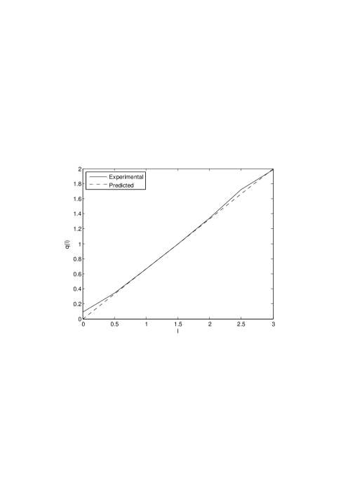
Figure 1. Plot of a numerical estimate of $q(\ell)$ against $\ell$ for the implicit midpoint rule applied to the semilinear wave equation, with the prediction of Theorem 5.3 for comparison.

In the rest of this section, equipped with the results of Section 4 on the stability of the semiflow and the numerical method under Galerkin, truncation we estimate the growth with $m$ of the local error of a Runge-Kutta method (3.1), subject to (RK1) and (RK2), applied to the projected equation (4.1) subject to (A) and (B) for non-smooth initial data. In this setting, by coupling $m$ and $h$ and balancing the projection error and trajectory error of the projected system, we obtain an estimate for $q(\ell)$ that describes the convergence of the numerical method for the semilinear evolution equation (1.1) as observed in Figure 1, see Section 5.2.

5.1. Preliminaries

We start with some preliminary lemmas.

Lemma 5.1 ($m$-dependent bounds for derivatives of $\Phi_{m}$).

Assume that the semilinear evolution equation (1.1) satisfies (A) and (B) and choose $\ell\in I^{-}$, $T>0$, $m_{*}\geq 0$ and $R>0$. Then for all $U^{0}$ with

$$\Phi^{t}_{m}(U^{0})\in\mathcal{B}_{\ell}^{R}\quad\mbox{for}\quad t\in[0,T],~{}~{}m\geq m_{*},$$ (5.3a)

and for all $$k\in\mathbb{N}_{0} k\leq\ell$$, we have

$$\Phi_{m}(U^{0})\in\mathcal{C}_{b}^{k}([0,T];\mathcal{B}_{0}^{R})$$ (5.3b)

with bounds uniform in $$U^{0} m\geq m_{*} k\in\mathbb{N}_{0} \ell\leq k\leq N U^{0} m U^{0} U^{0} \ell\leq k\leq N$$ and . Further, choose with . Then for all satisfying (5.3a), (5.3b) still holds, but with -dependent bounds which are uniform in . Moreover for all such , ,

$$\lVert\partial_{t}^{k}\Phi^{t}_{m}(U^{0})\rVert_{\mathcal{C}_{\operatorname{b}}([0,T];\mathcal{Y})}^{\vphantom{1}}=\mathcal{O}(m^{k-\ell}),$$ (5.3c)

with bounds uniform in $U^{0}$. The bounds and order constants only depend on $T$, $R$, (2.1) and the bounds from assumption (B).

Proof.

Due to Lemma 4.1 statement (5.3b) is non-trivial only if $\ell\geq 1$. In this case let $u_{m}(t)=\Phi_{m}^{t}(U^{0})$. From Lemma 4.1 with $\mathcal{Y}$ replaced by $\mathcal{Y}_{\ell}$, using (5.3b) we also get $u_{m}\in\mathcal{C}_{\operatorname{b}}([0,T];{\mathcal{B}^{R}_{\ell}})$. From (5.3a) and (4.1) we conclude that $\partial_{t}u_{m}\in\mathcal{C}_{\operatorname{b}}([0,T];{\mathcal{Y}_{\ell-1}})$ and thus, $u_{m}\in\mathcal{C}_{\operatorname{b}}([0,T];{\mathcal{Y}_{\ell}})\cap\mathcal{C}_{\operatorname{b}}^{1}([0,T];{\mathcal{B}_{\ell-1}^{R}})$ with bounds uniform in $m\geq m_{*}$ and $U^{0}$ satisfying (5.3a). That proves (5.3b) for $k=1$. If $\ell\geq 2$ then from (4.1) we get $\partial_{t}u_{m}\in\mathcal{C}_{\operatorname{b}}^{1}([0,T];{\mathcal{Y}_{\ell-2}})$ and therefore $u_{m}\in\mathcal{C}_{\operatorname{b}}^{2}([0,T];{\mathcal{B}_{\ell-2}^{R}})$. Inductively this proves that

$$\Phi_{m}(U^{0})\in\mathcal{C}_{\operatorname{b}}^{k}([0,T];\mathcal{B}_{\ell-k}^{R})$$ (5.4)

for $k\leq\ell$ with uniform bounds in $m\geq m_{*}$ and in all $U^{0}$ satisfying (5.3a). This proves (5.3b) for $k\leq\ell$ with $m$ independent bounds.

To prove (5.3c) we proceed by induction over $k=\lceil\ell\rceil,\ldots,N$. We consider the cases $\ell<1$ and $\ell\geq 1$ separately. If $\ell<1$ then from (4.1) we have

$$\|\partial_{t}u_{m}\|_{\mathcal{C}([0,T];\mathcal{Y})}\leq\|A_{m}u_{m}\|_{\mathcal{C}([0,T];\mathcal{Y})}+M\leq m^{1-\ell}\|u_{m}\|_{\mathcal{C}([0,T];\mathcal{Y}_{\ell})}+M=O(m^{1-\ell})$$

where $M=M_{0}[R]$, with order constant independent of $m\geq m_{*}$ and of $U^{0}$ satisfying (5.3a). This then immediately shows (5.3c) for $k=\lceil\ell\rceil=1$. If $\ell\geq 1$, $\ell\in\mathbb{Z}$ then the start of the induction is $k=\ell$, and the left hand side of (5.3c) is bounded by (5.3b).

If $\ell\geq 1$, $\ell\notin\mathbb{Z}$ then the start of the induction is $k=\lceil\ell\rceil>\ell$. Using (5.4) we can bound the $\lfloor\ell\rfloor$-th derivative independent of $m$ in the $\mathcal{Y}_{\ell-\lfloor\ell\rfloor}$ norm. Using the Faà di Bruno formula [5] we find that for any $i\in\mathbb{N}$, $i<N$,

$$\partial_{t}^{i+1}u_{m} =\partial_{t}^{i}(Au_{m}+B_{m}(u_{m}))$$

$$=A(\partial_{t}^{i}u_{m})+\sum_{1\leq\beta\leq i}\frac{i!\mathrm{D}^{\beta}_{u}B_{m}(u_{m})}{j_{1}!\cdots j_{i}!}\prod_{\alpha=1}^{i}\left(\frac{\partial_{t}^{\alpha}u_{m}}{\alpha!}\right)^{j_{\alpha}},$$ (5.5)

where $\beta=j_{1}+\cdots+j_{i}$ and the sum is over all $j_{\alpha}\in N_{0}$, $\alpha=1,\ldots,i$, with $j_{1}+2j_{2}+\cdots+ij_{i}=i$. We consider (5.5) with $i$ replaced by $\lfloor\ell\rfloor$. Then the second term in the last line of (5.5) is bounded independent of $m\geq m_{*}$ due to (5.3b). Furthermore, since $\partial_{t}^{\lfloor\ell\rfloor}u_{m}\in\mathcal{Y}_{\ell-\lfloor\ell\rfloor}$ by (5.4) with uniform bound in $m\geq m_{*}$, we estimate

$$\|A(\partial_{t}^{\lfloor\ell\rfloor}u_{m})\|_{\mathcal{Y}}=\|A^{1+\lfloor\ell\rfloor-\ell}(A^{\ell-\lfloor\ell\rfloor}\partial_{t}^{\lfloor\ell\rfloor}u_{m})\|_{\mathcal{Y}}=\mathcal{O}(m^{1+\lfloor\ell\rfloor-\ell}),$$

where we have used the first inequality of (2.4). So (5.3c) also holds true for $k=i+1=\lceil\ell\rceil$ when $\ell>1$, $\ell\notin\mathbb{Z}$.

Now fix an integer $k$ and assume that (5.3c) holds for all integers $i$ such that $\ell\leq i\leq k$. We now use (5.5) with $i=k$ to estimate $\|\partial_{t}^{k+1}u_{m}\|_{\mathcal{Y}}$. By the first inequality of (2.4) and the induction hypothesis the first term on the second line of (5.5) is $\mathcal{O}(m^{k+1-\ell})$. Moreover, by (5.3b) and the induction hypothesis, the $\mathcal{Y}$ norm of the second term is of order $\mathcal{O}(m^{n})$ with $n=0$ if $j_{\lceil\ell\rceil}+\ldots+j_{k}=0$ and

$$n=(\lceil\ell\rceil-\ell)j_{\lceil\ell\rceil}+\cdots+(k-\ell)j_{k}\leq k-\ell.$$

if $j_{\lceil\ell\rceil}+\ldots+j_{k}>0$. Thus we see that the right hand term of (5.5), with $i=k$, is $\mathcal{O}(m^{k+1-\ell})$ as well. ∎

Lemma 5.2 ($m$-dependent bounds for derivatives of $\Psi_{m}$ and $W_{m}$).

Assume that the semilinear evolution equation (1.1) satisfies (A) and (B), and apply a Runge-Kutta method subject to (RK1) and (RK2). Choose $\ell\in I^{-}$ and $k\in\mathbb{N}_{0}$ with $\ell\leq k\leq N$. Let $R>0$ and define $r$ as in (3.6b). Then there is $h_{*}>0$ such that for $m\geq 0$ and $i=1,\ldots,s$,

$$W_{m}^{i}(U,\cdot),\Psi_{m}(U,\cdot)\in\mathcal{C}_{b}^{k}([0,h_{*}];\mathcal{B}_{0}^{R})\quad\mbox{ for}\quad i=1,\ldots,s$$ (5.6)

with $m$-dependent bounds which are uniform in $U\in\mathcal{B}_{\ell}^{r}$. Moreover

$$\sup_{\begin{subarray}{c}U\in\mathcal{B}_{\ell}^{r}\\ h\in[0,h_{*}]\end{subarray}}\lVert\partial_{h}^{k}\Psi^{h}_{m}(U)\rVert_{\mathcal{Y}}^{\vphantom{1}}=\mathcal{O}(m^{k-\ell}),\quad\sup_{\begin{subarray}{c}U\in\mathcal{B}_{\ell}^{r}\\ h\in[0,h_{*}]\end{subarray}}\lVert\partial_{h}^{k}W_{m}(U,h)\rVert_{\mathcal{Y}^{s}}^{\vphantom{1}}=\mathcal{O}(m^{k-\ell}).$$ (5.7)

The order constants in (5.7) depend only $R$, (3.5d), $\mathsf{a}$ and $\mathsf{b}$ from the numerical method and the bounds afforded by (B) on balls of radius $R$.

Proof.

By Lemma 4.3, with $\mathcal{Y}$ replaced by $\mathcal{Y}_{\ell-j}$,

$$\Psi_{m},W_{m}^{i}\in\mathcal{C}_{b}^{j}([0,h_{*}];\mathcal{B}^{R}_{\ell-j}),$$ (5.8)

for $i=1,\ldots,s$, $j=1\ldots,\lfloor\ell\rfloor$, with bounds independent over $m\geq 0$ and $U\in\mathcal{B}^{r}_{\ell}$. From (3.3) we formally obtain

$$\partial_{h}^{k}\Psi_{m}^{h}(U,h)=\partial^{k}_{h}\mathsf{S}(hA)\mathbb{P}_{m}U+\sum_{j=0}^{k}{k\choose j}\mathsf{b}^{T}\partial^{k-j}_{h}(h(\operatorname{id}-h\mathsf{a}A)^{-1})\partial_{h}^{j}\mathbb{P}_{m}B(W_{m}(U,h)).$$ (5.9)

By (3.5c) and (2.4) there are $h_{*}>0$, $c_{\mathsf{S},k}$ such that for all $h\in[0,h_{*}]$ and $k\geq\ell$

$$\|\partial^{k}_{h}\mathsf{S}(hA)\mathbb{P}_{m}\|_{\mathcal{Y}_{\ell}\to\mathcal{Y}}\leq\|\partial^{k}_{h}\mathsf{S}(hA)\|_{\mathcal{Y}_{k}\to\mathcal{Y}}\|\mathbb{P}_{m}\|_{\mathcal{Y}_{\ell}\to\mathcal{Y}_{k}}\leq c_{\mathsf{S},k}m^{k-\ell}.$$ (5.10)

In addition (3.5d) shows that for $n\in\mathbb{N}$ with $n-1\geq\ell$

$$\|\partial^{n}_{h}(h(\operatorname{id}-h\mathsf{a}A)^{-1}\mathbb{P}_{m})\|_{\mathcal{Y}^{s}_{\ell}\to\mathcal{Y}^{s}} \leq\|\partial^{n}_{h}(h(\operatorname{id}-h\mathsf{a}A)^{-1})\|_{\mathcal{Y}^{s}_{n-1}\to\mathcal{Y}^{s}}\|\mathbb{P}_{m}\|_{\mathcal{Y}^{s}_{\ell}\to\mathcal{Y}^{s}_{n-1}}$$

$$\leq\frac{\Lambda_{n}}{\|\mathsf{a}\|}m^{n-1-\ell}.$$ (5.11)

Using (5.11) (with $\ell$ replaced by $\ell-j$ and $n$ by $k-j$) and (5.8), we can estimate the $j$-th term in the sum of (5.9) for $0\leq j\leq\ell\leq k$ as follows:

$$\| \partial^{k-j}_{h}(h(\operatorname{id}-h\mathsf{a}A)^{-1})\partial_{h}^{j}\mathbb{P}_{m}B(W_{m}(U,h))\|_{\mathcal{Y}^{s}}$$

$$\leq\|\partial^{k-j}_{h}(h(\operatorname{id}-h\mathsf{a}A)^{-1})\mathbb{P}_{m}\|_{\mathcal{Y}^{s}_{\ell-j}\to\mathcal{Y}^{s}}\|\partial_{h}^{j}B(W_{m}(U,h))\|_{\mathcal{Y}_{\ell-j}^{s}}$$

$$\leq O(m^{k-\ell}).$$ (5.12)

To obtain the first estimate of (5.7) assume that there is $b_{j}>0$ such that

$$\|\partial_{h}^{j}\mathbb{P}_{m}B(W_{m}(U,h))\|_{\mathcal{Y}}\leq b_{j}m^{j-\ell}$$ (5.13)

for all $h\in[0,h_{*}]$, $U\in\mathcal{B}^{r}_{\ell}$ and $k\geq j\geq\ell$. This will be proved below. Then, using (5.11) and (5.13) we can estimate the $j$-th term in the sum of (5.9) for $j\geq\ell$ as follows:

$$\|\partial^{k-j}_{h} (h(\operatorname{id}-h\mathsf{a}A)^{-1})\partial_{h}^{j}\mathbb{P}_{m}B(W_{m}(U,h))\|_{\mathcal{Y}^{s}}$$

$$\leq\|\partial^{k-j}_{h}(h(\operatorname{id}-h\mathsf{a}A)^{-1})\mathbb{P}_{m}\|_{\mathcal{Y}^{s}\to\mathcal{Y}^{s}}\|\partial_{h}^{j}B(W_{m}(U,h))\|_{\mathcal{Y}^{s}}$$

$$\leq\frac{\Lambda_{k-j}}{\|\mathsf{a}\|}m^{k-j}b_{j}m^{j-\ell}=O(m^{k-\ell}).$$ (5.14)

These estimates, with (5.9) and (5.10), then prove the first estimate of (5.7).

To prove (5.13) and the second estimate of (5.7), differentiate (3.2) $k$ times in $h$:

$$\partial_{h}^{k}W_{m}=\partial_{h}^{k}(\operatorname{id}-h\mathsf{a}A)^{-1}\mathbbm{1}\mathbb{P}_{m}U+\sum_{j=0}^{k}{k\choose j}\partial_{h}^{k-j}(h\mathsf{a}(\operatorname{id}-h\mathsf{a}A)^{-1}\mathbb{P}_{m})\partial_{h}^{j}B(W_{m}).$$ (5.15)

By (3.5d) and (2.4), for $k\geq\ell$,

$$\sup_{h\in[0,h_{*}]}\|\partial_{h}^{k}(\operatorname{id}-h\mathsf{a}A)^{-1}\mathbbm{1}\mathbb{P}_{m}\|_{\mathcal{Y}_{\ell}^{s}\to\mathcal{Y}^{s}}\leq\Lambda_{k}m^{k-\ell}.$$ (5.16)

Now we show inductively the second estimate of (5.7) and estimate (5.13) for $k=\lceil\ell\rceil,\ldots,N$. If $\ell\in\mathbb{N}_{0}$ then the start of the induction is $k=\ell$, and the required estimates are given by Theorem 4.3. If $\ell\notin\mathbb{N}_{0}$, then the start of the induction is $k=\lceil\ell\rceil>\ell$. If $k=\lceil\ell\rceil$ then, due to (5.16), the first term in (5.15) is of order $\mathcal{O}(m^{k-\ell})$, and all other terms in the sum of (5.15) are bounded due to (3.5d) and (5.8) except when $j=k$ in the sum. Hence, using (3.5b),

$$\sup_{\begin{subarray}{c}h\in[0,h_{*}]\\ U\in\mathcal{B}^{r}_{\ell}\end{subarray}}\|\partial_{h}^{k}W_{m}(U,h)\|_{\mathcal{Y}^{s}}\leq\mathcal{O}(m^{k-\ell})+\Lambda\|\mathsf{a}\|h_{*}\sup_{\begin{subarray}{c}h\in[0,h_{*}]\\ U\in\mathcal{B}^{r}_{\ell}\end{subarray}}\|\partial_{h}^{k}B(W_{m}(U,h))\|_{\mathcal{Y}^{s}}.$$ (5.17)

Now we use the Faà di Bruno formula (5.5) again:

$$\partial_{h}^{k}B(W_{m}(U,h))=\sum_{1\leq\beta\leq k}\frac{k!\mathrm{D}^{\beta}_{w}B_{m}(W_{m}(U,h))}{j_{1}!\cdots j_{k}!}\prod_{\alpha=1}^{k}\left(\frac{\partial_{h}^{\alpha}W_{m}(U,h)}{\alpha!}\right)^{j_{\alpha}}$$ (5.18)

where $\beta=j_{1}+\cdots+j_{k}$ and the sum is over all $j_{\alpha}\in N_{0}$, $\alpha=1,\ldots,k$ with $j_{1}+2j_{2}+\cdots kj_{k}=k$. We see that all terms on the right hand side of (5.18) contain $h$-derivatives of order at most $k-1$ and are therefore bounded and in particular $\mathcal{O}(m^{k-\ell})$, except when $\beta=j_{k}=1$ and $j_{\alpha}=0$ for $\alpha\neq k$. So we obtain

$$\sup_{\begin{subarray}{c}h\in[0,h_{*}]\\ U\in\mathcal{B}^{r}_{\ell}\end{subarray}}\|\partial_{h}^{k}B(W_{m}(U,h))\|_{\mathcal{Y}^{s}} \leq\mathcal{O}(m^{k-\ell})+\sup_{\begin{subarray}{c}h\in[0,h_{*}]\\ U\in\mathcal{B}^{r}_{\ell}\end{subarray}}\|\mathrm{D}B(W_{m}(U,h))\partial_{h}^{k}W_{m}(U,h)\|_{\mathcal{Y}^{s}}$$

$$\leq\mathcal{O}(m^{k-\ell})+M^{\prime}_{0}[R]\sup_{\begin{subarray}{c}h\in[0,h_{*}]\\ U\in\mathcal{B}^{r}_{\ell}\end{subarray}}\|\partial_{h}^{k}W_{m}(U,h)\|_{\mathcal{Y}^{s}}.$$ (5.19)

Substituting this into (5.17) gives the second estimate of (5.7) for $k=\lceil\ell\rceil$ and $h_{*}$ small enough. Resubstituting this estimate into (5.19) also shows (5.13) for $k=\lceil\ell\rceil$.

Now assume these estimates hold true for all $\hat{k}\in N_{0}$ with $\ell\leq\hat{k}\leq k-1$ and let $k\leq N$. Then, using the induction hypothesis and the above estimates, in particular (5.12), (5.13), (5.14) and (5.16), all terms in (5.15) are $\mathcal{O}(m^{k-\ell})$ except when $j=k$ in the sum. We deduce that (5.17) remains valid under the induction hypothesis. Moreover, by the induction hypothesis, each term in the sum of the Faà di Bruno formula (5.18) with $j_{k}=0$ is of order $\mathcal{O}(m^{n})$ with $n=0$ if $j_{\lceil\ell\rceil}+\ldots+j_{k-1}=0$ and

$$n=(\lceil\ell\rceil-\ell)j_{\lceil\ell\rceil}+\cdots+(k-1-\ell)j_{k-1}\leq k-\ell$$

if $j_{\lceil\ell\rceil}+\ldots+j_{k-1}>0.$ Hence (5.19) remains valid, and we deduce (5.13) and the second estimate of (5.7) as before. ∎

5.2. Trajectory error for nonsmooth data

Now we are ready to prove our main result:

Theorem 5.3 (Trajectory error for nonsmooth data).

Assume that the semilinear evolution equation (1.1) satisfies (A) and (B) and apply a Runge-Kutta method (3.1) subject to (RK1) and (RK2). Let $\ell\in I^{-}$, $0<\ell\leq p+1$, and fix $T>0$ and $R>0$. Then there exist constants $h_{*}>0$, $c_{1}>0$, $c_{2}>0$ such that for every $U^{0}$ with

$$\|\Phi^{t}(U^{0})\|_{\mathcal{Y}_{\ell}}\leq R,\quad\mbox{for}~{}~{}t\in[0,T]$$ (5.20)

and for all $h\in[0,h_{*}]$ we have

$$\|\Phi^{nh}(U^{0})-(\Psi^{h})^{n}(U^{0})\|_{\mathcal{Y}}\leq c_{1}e^{c_{2}nh}h^{p\ell/(p+1)},$$ (5.21)

provided that $nh\leq T$. The constants $h_{*}$, $c_{1}$ and $c_{2}$ depend only on $R$, $T$, (2.1), (3.5d), $\mathsf{a}$, $\mathsf{b}$ from the numerical method and the bounds afforded by (B).

Proof of Theorem 5.3. The proof consists of several steps, as outlined in the diagram below:

Solution of the PDE	Error to be estimated	RK solution of PDE
Projection error $\downarrow$		Projection error $\uparrow$
Solution of projected PDE	$\longrightarrow$	RK solution of projected PDE
	Numerical scheme error

We want to estimate the error of the Runge Kutta time discretization of the evolution equation (first line of the diagram). To do this, in a first step, we discretize in space by a Galerkin truncation. We estimate the projection error and prove regularity of the solution $u_{m}(t)$ of the projected system (first column in the diagram). In the second step of the proof we investigate the error of the time discretization of the space-discretized system (third row in the diagram) and couple the spatial discretization parameter $m$ with the time step size $h$ in suitable way. In the third step of the proof (third column of the diagram) we prove regularity of the space-time discretization and estimate the projection error of the Runge Kutta time discretization. This concludes the proof.

Step 1 (Regularity of solution of the projected system) In a first step we aim to prove regularity of the continuous solution of the projected system $u_{m}(t)=\phi_{m}^{t}(\mathbb{P}_{m}U^{0})=\Phi_{m}^{t}(U^{0})$ which will be needed later. For the proof we denote $R$ from (5.20) as $R_{\Phi}$ to indicate that it is a bound on $\Phi^{t}(U^{0})$. We will prove that there is some $r_{\phi}>0$ such that

$$\|\phi_{m}^{t}(\mathbb{P}_{m}U^{0})\|_{\mathcal{Y}_{\ell}}\leq r_{\phi}$$ (5.22)

uniformly in $U^{0}$ satisfying (5.20) and $m\geq m_{*}$, $t\in[0,T]$, where $m_{*}\geq 0$ is sufficiently large. Fix $\delta>0$. Then we have

$$\|\Phi_{m}^{t}(U^{0}))\|_{\mathcal{Y}_{\ell}} \leq\|\mathbb{P}_{m}\Phi^{t}(U^{0})-\Phi_{m}^{t}(U^{0})\|_{\mathcal{Y}_{\ell}}+\|\mathbb{P}_{m}\Phi^{t}(U^{0})\|_{\mathcal{Y}_{\ell}}$$

$$\leq m^{\ell}\|\mathbb{P}_{m}\Phi^{t}(U^{0})-\Phi_{m}^{t}(U^{0})\|_{\mathcal{Y}}+\|\Phi^{t}(U^{0})\|_{\mathcal{Y}_{\ell}}$$

$$\leq R_{\Phi}\mathrm{e}^{(\omega+M^{\prime})t}+R_{\Phi}=r_{\phi}$$ (5.23)

for $U^{0}$ satisfying (5.20) and $m\geq m_{*}$. Here $M^{\prime}=M^{\prime}_{0}[R_{\Phi}+\delta]$ and we used (2.4) in the second estimate and Lemma 4.2 and (5.20) in the final estimate. This proves (5.22).

Step 2 (Trajectory error of the time discretized projected system) Next we aim to estimate the trajectory error of the time discretization of the projected system. First note that by Theorem 4.3 (with $r$ replaced by $2r_{\phi}$ and consequently $R$ by $4r_{\phi}\Lambda$) there is $h_{*}>0$ such that for $m\geq 0$, $h\in[0,h_{*}]$ we have $W^{i}_{h},\Psi^{h}_{m}\in\mathcal{C}_{\operatorname{b}}^{1}(\mathcal{B}^{2r_{\phi}}_{0};\mathcal{Y})$, $i=1,\ldots,s$, with uniform bounds in $m\geq 0$, $h\in[0,h_{*}]$. Moreover, using (3.3), (3.5a) and (3.5b) we obtain the following bound for $h\in[0,h_{*}]$ to be used later:

$$\sup_{U\in\mathcal{B}^{2r_{\phi}}_{0}}\|\mathrm{D}\Psi_{m}^{h}(U)\|_{\mathcal{Y}\to\mathcal{Y}} \leq\|\mathsf{S}(hA)\|_{\mathcal{Y}\to\mathcal{Y}}+h\Lambda\|\mathsf{b}\|M^{\prime}\|W_{m}^{\prime}(U)\|_{\mathcal{Y}\to\mathcal{Y}^{s}}$$

$$\leq 1+\sigma h+h\Lambda\|\mathsf{b}\|M^{\prime}\|W_{m}^{\prime}(U)\|_{\mathcal{Y}\to\mathcal{Y}^{s}}=:1+\sigma_{\Psi}h.$$ (5.24)

where $M^{\prime}=M^{\prime}_{0}[4r_{\phi}\Lambda]$.

Now we define the global error of the projected system, for $jh\leq T$,

$$E_{m}^{j}(U^{0},h)=\lVert\Phi^{jh}_{m}(U^{0})-(\Psi^{h}_{m})^{j}(U^{0})\rVert_{\mathcal{Y}}^{\vphantom{1}}.$$ (5.25)

We estimate for any $U^{0}$ satisfying (5.20) and for all $(n+1)h\leq T$, $h\in[0,h_{*}]$, $m\geq m_{*}$,

$$E_{m}^{n+1}( U^{0},h)=\lVert\Phi^{(n+1)h}_{m}(U^{0})-(\Psi^{h}_{m})^{n+1}(U^{0})\rVert_{\mathcal{Y}}^{\vphantom{1}}$$

$$\leq\lVert\Phi^{h}_{m}(\Phi_{m}^{nh}(U^{0}))-\Psi^{h}_{m}(\Phi_{m}^{nh}(U^{0}))\rVert_{\mathcal{Y}}^{\vphantom{1}}+\lVert\Psi^{h}_{m}(\Phi_{m}^{nh}(U^{0}))-\Psi^{h}_{m}((\Psi^{h}_{m})^{n}(U^{0}))\rVert_{\mathcal{Y}}^{\vphantom{1}}$$

$$\leq\frac{h^{p+1}}{(p+1)!}\sup_{\tau\in[0,h]}\left(\lVert\partial_{\tau}^{p+1}\Phi^{\tau}_{m}(\Phi_{m}^{nh}(U^{0}))\rVert_{\mathcal{Y}}^{\vphantom{1}}+\lVert\partial_{\tau}^{p+1}\Psi^{\tau}_{m}(\Phi_{m}^{nh}(U^{0})))\rVert_{\mathcal{Y}}^{\vphantom{1}}\right)$$

$$+\sup_{\theta\in[0,1]}\lVert\mathrm{D}\Psi^{h}_{m}(\Phi_{m}^{nh}(U^{0})+\theta((\Psi^{h}_{m})^{n}(U^{0})-\Phi_{m}^{nh}(U^{0})))\rVert_{\mathcal{Y}\to\mathcal{Y}}^{\vphantom{1}}\cdot E_{m}^{n}(U^{0},h)$$ (5.26a)

$$\leq\frac{h^{p+1}}{(p+1)!}\left(\sup_{t\in[0,T]}\lVert\partial_{t}^{p+1}\Phi_{m}^{t}(U^{0})\rVert_{\mathcal{Y}}^{\vphantom{1}}+\sup_{t\in[0,T]}\sup_{h\in[0,h_{*}]}\lVert\partial_{h}^{p+1}\Psi^{h}_{m}(\Phi_{m}^{t}(U^{0}))\rVert_{\mathcal{Y}}^{\vphantom{1}}\right)$$

$$\quad+\sup_{U\in\mathcal{B}^{2r_{\phi}}_{0}}\lVert\mathrm{D}\Psi^{h}_{m}(U)\rVert_{\mathcal{Y}\to\mathcal{Y}}^{\vphantom{1}}\cdot E_{m}^{n}(U^{0},h)$$ (5.26b)

$$\leq\rho h^{p+1}m^{p+1-\ell}+(1+\sigma_{\Psi}h)E_{m}^{n}(U^{0},h),$$

for some $\rho>0$. Due to (5.24), the second lines of (5.26a) and (5.26b) are valid as long as

$$\Phi_{m}^{nh}(U^{0})+\theta((\Psi^{h}_{m})^{n}(U^{0})-\Phi_{m}^{nh}(U^{0}))\in\mathcal{B}_{0}^{2r_{\phi}},\quad\theta\in[0,1],nh\leq T,h\in[0,h_{*}].$$ (5.27)

Moreover the first supremum of (5.26b) is $O(m^{p+1-\ell})$ by Lemma 5.1, with $R$ replaced by $r_{\phi}$. The second supremum of (5.26b) is $O(m^{p+1-\ell})$ by Lemma 5.2, with $\mathcal{B}^{r}_{\ell}$ replaced by $\mathcal{B}_{\ell}^{r_{\phi}}$ (and $R$ replaced by $2r_{\phi}\Lambda$).

Clearly $E_{m}^{0}(U,h)=0$, so

$$E_{m}^{n}(U,h) \leq\rho h^{p+1}m^{p+1-\ell}\frac{(1+\sigma_{\Psi}h)^{n}-1}{\sigma_{\Psi}h}$$

$$\leq\frac{\rho}{\sigma_{\Psi}}h^{p}m^{p+1-\ell}\left(1+\frac{n\sigma_{\Psi}h}{n}\right)^{n}\leq\frac{\rho}{\sigma_{\Psi}}h^{p}m^{p+1-\ell}e^{n\sigma_{\Psi}h}.$$

Choosing $m(h)=h^{-p/(p+1)}$ we see that for $nh\leq T$, $h\in[0,h_{*}]$,

$$\|(\Psi^{h}_{m})^{n}(U^{0})-\Phi^{nh}_{m}(U^{0})\|_{\mathcal{Y}}\leq\frac{\rho}{\sigma_{\Psi}}\mathrm{e}^{\sigma_{\Psi}T}h^{p}m^{p+1-\ell}=C\mathrm{e}^{\sigma_{\Psi}T}h^{\ell p/(p+1)}.$$ (5.28)

Using (5.28) we can ensure that for $nh\leq T$, $h\in[0,h_{*}]$

$$\|(\Psi^{h}_{m})^{n}(U^{0})-\Phi^{nh}_{m}(U^{0})\|_{\mathcal{Y}}\leq r_{\phi}$$ (5.29)

by possibly reducing $h_{*}>0$, and hence that (5.27) holds.

Step 3 (Projection error of numerical trajectory) We now estimate the global projection error of the numerical method. We will prove that for $m(h)=h^{-p/(p+1)}$, $nh\leq T$, $h\in[0,h_{*}]$,

$$\|(\Psi^{h})^{n}(U^{0})-(\Psi_{m(h)}^{h})^{n}(U^{0})\|_{\mathcal{Y}}=\mathcal{O}(m^{-\ell})$$ (5.30)

uniformly for initial data $U^{0}$ satisfying (5.20).

We first establish the required regularity of the numerical trajectory of the projected system: To bound the $\mathcal{Y}_{\ell}$-norm of the Galerkin truncated numerical trajectory $(\Psi^{h}_{m(h)})^{n}(U^{0})$ note that for $m=m(h)=h^{-p/(p+1)}$, $nh\leq T$, $h\in[0,h_{*}]$, with $h_{*}$ small enough such that $m(h_{*})\geq m_{*}$, we have

$$\|(\Psi_{m(h)}^{h})^{n}(U^{0})\|_{\mathcal{Y}_{\ell}} \leq\|(\Psi^{h}_{m})^{n}(U^{0})-\Phi^{nh}_{m}(U^{0})\|_{\mathcal{Y}_{\ell}}+\|\Phi^{nh}_{m}(U^{0})\|_{\mathcal{Y}_{\ell}}$$

$$\leq m^{\ell}\|(\Psi^{h}_{m})^{n}(U^{0})-\Phi^{nh}_{m}(U^{0})\|_{\mathcal{Y}}+r_{\phi}$$

$$\leq m^{\ell}(C\mathrm{e}^{\sigma_{\Psi}T}m^{p+1-\ell}h^{p})+r_{\phi}\leq C\mathrm{e}^{\sigma_{\Psi}T}+r_{\phi}\leq r_{\psi}$$ (5.31)

for some $r_{\psi}>0$. Here $r_{\phi}$ is as in (5.22) and we used (2.4) in the second line and (5.28) in the third line.

To prove (5.30) let

$$e^{j}(U^{0})=(\Psi^{h})^{j}(U^{0})-(\Psi^{h}_{m})^{j}(U^{0})$$

be the truncation error at time $jh\leq T$. Then for $(n+1)h\leq T$,

$$e^{n+1}(U^{0}) =(\Psi^{h}\circ(\Psi^{h})^{n})(U^{0})-(\Psi^{h}\circ(\Psi^{h}_{m})^{n})(U^{0})$$

$$+(\Psi^{h}\circ(\Psi^{h}_{m})^{n})(U^{0})-(\Psi^{h}_{m}\circ(\Psi^{h}_{m})^{n})(U^{0}).$$ (5.32)

By Theorem 4.3, with $r$ replaced by $2r_{\psi}$ (and consequently $R$ by $4r_{\psi}\Lambda$, see (3.6b)) we have

$$\Psi_{m}\in\mathcal{C}_{\operatorname{b}}^{1}(\mathcal{B}_{0}^{2r_{\psi}};\mathcal{Y}).$$ (5.33)

By (5.24), with $\Psi_{m}$ replaced by $\Psi$ and the supremum taken over $\mathcal{B}_{0}^{2r_{\psi}}$, using (5.33) we get from (5.32) for $n\geq 1$, $h\in[0,h_{*}]$ and $(n+1)h\leq T$ that

$$\|e^{n+1}(U^{0})\|_{\mathcal{Y}} \leq\sup_{\theta\in[0,1]}\|\mathrm{D}\Psi^{h}((\Psi^{h}_{m})^{n}+\theta((\Psi^{h})^{n}-(\Psi^{h}_{m})^{n})(U^{0}))\|_{\mathcal{Y}\to\mathcal{Y}}\|e^{n}(U^{0})\|_{\mathcal{Y}}$$

$$+\|e^{1}((\Psi^{h}_{m})^{n}(U^{0}))\|_{\mathcal{Y}}$$

$$\leq\sup_{\|U\|_{\mathcal{Y}_{\ell}}\leq 2r_{\psi}}\|\mathrm{D}\Psi^{h}(U)\|_{\mathcal{Y}\to\mathcal{Y}}\|e^{n}(U^{0})\|_{\mathcal{Y}}+\|e^{1}((\Psi^{h}_{m})^{n}(U^{0}))\|_{\mathcal{Y}}$$

$$\leq(1+\sigma_{\Psi}h)\|e^{n}(U^{0})\|_{\mathcal{Y}}+h\mathcal{O}(m^{-\ell}),$$ (5.34)

where $m=m(h)$, with order constant uniformly in all $U^{0}$ satisfying (5.20), as long as

$$(\Psi^{h}_{m})^{n}(U^{0})+\theta((\Psi^{h})^{n}(U^{0})-(\Psi^{h}_{m})^{n}(U^{0}))\in\mathcal{B}_{0}^{2r_{\psi}},\quad\theta\in[0,1].$$ (5.35)

Here we used that for $U\in\mathbb{P}_{m}\mathcal{Y}$,

$$e^{1}(U)=h\mathsf{b}^{T}(\operatorname{id}-h\mathsf{a}A)^{-1}\left(\left(\mathbb{P}_{m}(B(W(U,h))-B(W_{m}(U,h))\right)+\mathbb{Q}_{m}B(W(U,h))\right),$$

so that for $U\in\mathcal{B}_{\ell}^{r_{\psi}}\cap\mathbb{P}_{m}\mathcal{Y}$, $h\in[0,h_{*}]$, by (4.5c) (with $r$ replaced by $r_{\psi}$ and $R$ by $2r_{\psi}\Lambda$)

$$\|e^{1}(U)\|_{\mathcal{Y}} \leq h\|\mathsf{b}\|\Lambda(M^{\prime}\|W(U,h)-W_{m}(U,h)\|_{\mathcal{Y}^{s}}+\|\mathbb{Q}_{m}B(W(U,h))\|_{\mathcal{Y}^{s}})$$

$$\leq h\|\mathsf{b}\|(\Lambda M^{\prime}\mathcal{O}(m^{-\ell})+\mathcal{O}(m^{-\ell}))=h\mathcal{O}(m^{-\ell}),$$ (5.36)

where $m=m(h)$ and $M^{\prime}=M_{0}^{\prime}[2r_{\psi}\Lambda]$. In the last inequality of (5.36) we used that

$$\|\mathbb{Q}_{m}B(W(U,h))\|_{\mathcal{Y}^{s}}\leq m^{-\ell}M=\mathcal{O}(m^{-\ell}),$$ (5.37)

where $M=M_{0}[2r_{\psi}\Lambda]$.

From (5.34) we deduce for $nh\leq T$, $h\in[0,h_{*}]$ and all $U^{0}$ satisfying (5.20) that

$$\|e^{n}(U^{0})\|_{\mathcal{Y}} \leq(1+\sigma_{\Psi}h)^{n-1}\|e^{1}(U^{0})\|_{\mathcal{Y}}+\frac{1}{\sigma_{\Psi}h}\left((1+\sigma_{\Psi}h)^{n-1}-1\right)h\mathcal{O}(m^{-\ell})$$

$$\leq\exp(\sigma_{\Psi}T)(\|e^{1}(U^{0})\|_{\mathcal{Y}}+\mathcal{O}(m^{-\ell}))=\mathcal{O}(m^{-\ell}),$$ (5.38)

with $m=m(h)$. Here (5.36) does not apply to $\|e^{1}(U^{0})\|_{\mathcal{Y}}$ because in general $U^{0}\notin\mathbb{P}_{m}\mathcal{Y}$. But from (4.5d) we see that $\|e^{1}(U^{0})\|_{\mathcal{Y}}=O(m^{-\ell})$. By choosing a possibly bigger $m_{*}$ (and, by virtue of $m=h^{-p/(p+1)}$, a smaller $h_{*}$) we can achieve that $\|e^{n}(U^{0})\|_{\mathcal{Y}}\leq r_{\psi}$ so that the required condition (5.35) is satisfied. This proves (5.30).

Hence, (4.3b), (5.28) and (5.30) prove that

$$E^{n}(U^{0},h)=E_{m}^{n}(U^{0},h)+\mathcal{O}(m^{-\ell})=\mathcal{O}(h^{p\ell/(p+1)})$$ (5.39)

for $nh\leq T$, $h\in[0,h_{*}]$ and $U^{0}$ satisfying (5.20). ∎

Example 5.4.

(Cubic nonlinear Schrödinger equation in $\mathbb{R}^{3}$) We now consider a cubic nonlinear Schrödinger equation in $\mathbb{R}^{3}$

$$\mathrm{i}u_{t}=\Delta u+|u|^{2}u$$ (5.40)

as in [13]. We rewrite it in the form (1.1) with $U=(u_{1},u_{2})$ where $u=u_{1}+\mathrm{i}u_{2}$ with

$$A=\left(\begin{array}[]{cc}0&\Delta\\ -\Delta&0\\ \end{array}\right),\quad\mbox{and}\quad B(U)=(u_{1}^{2}+u_{2}^{2}){u_{2}\choose-u_{1}},$$

cf. also Example 2.8, and consider it on $\mathcal{Y}=\mathcal{H}_{2}(\mathbb{R}^{3};\mathbb{R}^{2})$. By Lemma 2.9 a) the nonlinearity $B(U)$ is analytic on $\mathcal{Y}$ and the same holds true on $\mathcal{Y}_{\ell}=D(A^{\ell})=\mathcal{H}_{2(\ell+1)}(\mathbb{R}^{3},\mathbb{R}^{2})$ where $\ell\geq 0$. In this case assumption (B) holds for $I=[0,L]$ and any $L>0$. If (5.40) is discretized by the implicit mid point rule and $U^{0}\in\mathcal{Y}_{1}=\mathcal{H}_{4}$, then from Theorem 5.3 we obtain an order of convergence $\mathcal{O}(h^{2/3})$ in the $\mathcal{H}_{2}$-norm. In [13] a second order Strang type time discretization is used to discretize (5.40) and a better rate of convergence is observed, namely an order of convergence $\mathcal{O}(h)$ in the $\mathcal{H}_{2}$-norm for $U^{0}\in\mathcal{H}_{4}$. This is due to the fact that the linear part of the evolution equation (1.1), i.e., $\dot{U}=AU$, is integrated exactly by this method. We plan to extend the methods of this paper to splitting and exponential integrators in future work.

6. Appendix: Trajectory error on general domains

In this appendix we show how to extend the results of this paper to more general domains. We make the following assumption for the nonlinearity $B(U)$ of the semilinear evolution equation (1.1):

1. There exists $L\geq 0$, $I\subseteq[0,L]$, $0,L\in I$, $N\in\mathbb{N}$, $N>\lceil L\rceil$ and a nested collection of open, $\mathcal{Y}_{\ell}$-bounded sets $\mathcal{D}_{\ell}\subset\mathcal{Y}_{\ell}$, $\ell\in I$, such that $B\in\mathcal{C}_{\operatorname{b}}^{N-\lceil\ell\rceil}(\mathcal{D}_{\ell};\mathcal{Y}_{\ell})$ for $\ell\in I$.

Similarly as before we denote the supremum of $B:\mathcal{D}_{\ell}\to\mathcal{Y}_{\ell}$ as $M_{\ell}$ and the supremum of its derivative as $M^{\prime}_{\ell}$, and set $M=M_{0}$, $M^{\prime}=M^{\prime}_{0}$ and $\mathcal{D}=\mathcal{D}_{0}$.

The right hand side of the evolution equation (1.1) is bounded in the $\mathcal{Y}$ norm for $U\in\mathcal{D}\cap D(A)$ and it is well-known that there exists a differentiable solution $\Phi^{t}(U)\in\mathcal{Y}$ in this case, see [17] and Theorem 6.1 below. Extending this setting we will in this section consider initial data $U^{0}\in\mathcal{Y}_{\ell}$ with $\ell\in J^{-}$ defined as follows:

$$J^{-}:=\{\ell\in J:\ell-k\in I,k=1,\ldots,\lfloor\ell\rfloor\},\quad\mbox{where}\quad J=I\cup[L,L+1],$$ (6.1)

similarly as in (2.7). For our main result, Theorem 6.10 below, we need an additional condition on the nonlinearity $B$ of (1.1).

1. $B:\mathcal{D}_{[\ell-1]^{+}}\cap\mathcal{B}_{\ell}^{R}\to\mathcal{Y}_{\ell}$ is bounded for any $\ell>0$ with $\ell\in J^{-}$ and any $R>0$.

Here we define $[x]^{+}=\max(x,0)$ for $x\in\mathbb{R}$. Assumption (B2) is often satisfied for superposition operators, see Lemma 2.9 b), c) and in particular Example 2.4 where the potential $V$ of the semilinear wave equation is only defined on an open subset $D$ of $\mathbb{R}$.

For a subset $\mathcal{U}$ of some Hilbert space $\mathcal{Y}$ and $\delta>0$ we denote by

$$\mathcal{U}^{\delta}=\bigcup_{u\in\mathcal{U}}\mathcal{B}_{\mathcal{Y}}^{\delta}(u)$$

a $\delta$-neighbourhood of $\mathcal{U}$. Moreover for any subset $\mathcal{U}_{\ell}$ of $\mathcal{Y}_{\ell}$, $\ell\in I$, we define $(\mathcal{U}_{\ell})^{\delta}_{\ell}=\mathcal{U}_{\ell}^{\delta}$ as a $\delta$-neighbourhood of $\mathcal{U}_{\ell}$ in $\mathcal{Y}_{\ell}$. In the following let $\mathcal{U}_{\ell}\subseteq\mathcal{D}_{\ell}$, $\ell\in I$, be a nested collection of open sets and $\delta>0$ be such that

$$\mathcal{U}_{\ell}^{\delta}\subseteq\mathcal{D}_{\ell},\quad\ell\in I.$$ (6.2)

We will also frequently use the abbreviation

$$\widehat{\mathcal{U}}_{\ell}:=\mathcal{U}_{[\ell-1]^{+}}\cap\mathcal{B}_{\ell}^{R}$$ (6.3)

for $\ell\in J$.

To extend Theorem 2.2 (and also Theorem 3.3, see below) to general domains we cover the domain $\mathcal{U}_{\ell}$ with open balls of radius $\delta$ and apply the corresponding theorems on each ball. To ensure uniformity of the maximal time interval of existence $T_{*}$ we consider initial data in $(\widehat{\mathcal{U}}_{\ell})^{\delta/2}_{0}$.

Theorem 6.1 (Regularity of the semiflow on general domains).

Assume (A) and (B1) and choose $\ell>0$. Then there is $T_{*}>0$ such that

$$\Phi^{t}\in\mathcal{C}_{\operatorname{b}}^{N}((\widehat{\mathcal{U}}_{\ell})^{\delta/2}_{0};\mathcal{D})$$ (6.4a)

with uniform bounds in $$t\in[0,T_{*}] \ell\in J^{-} k\in\mathbb{N}_{0} k\leq\ell$$. Moreover if and satisfies , then

$$\Phi(U)\in\mathcal{C}_{\operatorname{b}}^{k}([0,T_{*}];\mathcal{D})$$ (6.4b)

with uniform bounds in $$U\in\widehat{\mathcal{U}}_{\ell}$$.

The bounds on $T_{*}$ and $\Phi$, depend only on $\delta$ from (6.2), $R$ from (6.3), $\omega$ from (2.1), and those afforded by assumption (B1).

Proof.

The proof is a modification of the proof of Theorem 2.2. Here we let $U^{0}\in\widehat{\mathcal{U}}_{\ell}$ and take $R=\delta$. As before we compute $W$ as fixed point of the map $\Pi$ from (2.9), but this time we consider $\Pi$ as map from $\mathcal{B}^{\delta}_{\mathcal{Z}}(U^{0})\times\mathcal{B}^{\delta/2}_{\mathcal{Y}}(U^{0})\times[0,T_{*}]$ to $\mathcal{Z}$ noting that by (6.2) we have $\mathcal{B}^{\delta}_{\mathcal{Y}}(U^{0})\subseteq\mathcal{D}$. Then (2.10) becomes

$$\|\Pi(W,U,T)-U^{0}\|_{\mathcal{Z}}\leq\max_{\tau\in[0,1]}\|\mathrm{e}^{\tau TA}(U-U^{0})\|_{\mathcal{Y}}+\max_{\tau\in[0,1]}\|(\mathrm{e}^{\tau TA}-1)U^{0}\|_{\mathcal{Y}}+T\mathrm{e}^{\omega T}M$$ (6.5)

and, for $0<\epsilon\leq\min(1,\ell)$, we estimate the additional term as follows

$$\max_{\tau\in[0,1]}\|(\mathrm{e}^{\tau TA}-\operatorname{id})U^{0}\|_{\mathcal{Y}}\leq\max_{\tau\in[0,1]}\|(\mathrm{e}^{\tau TA}-\operatorname{id})\|_{\mathcal{Y}_{\epsilon}\to\mathcal{Y}}\|U^{0}\|_{\mathcal{Y}_{\epsilon}}\leq cT^{\epsilon}\|U^{0}\|_{\mathcal{Y}_{\epsilon}}$$

uniform in $U^{0}\in\widehat{\mathcal{U}}_{\ell}$. Here we have used Lemma 6.2 below and that $\|U^{0}\|_{\mathcal{Y}_{\epsilon}}\leq\|U^{0}\|_{\mathcal{Y}_{\ell}}\leq R$ for $U^{0}\in\widehat{\mathcal{U}}_{\ell}$. Hence for $T_{*}>0$ sufficiently, $\Pi(\cdot,U,T)$ maps $\mathcal{B}^{\delta}_{\mathcal{Z}}(U^{0})$ into itself and, similarly as before, $W\in\mathcal{C}_{\operatorname{b}}(\mathcal{B}^{\delta/2}_{\mathcal{Y}}(U^{0})\times[0,T_{*}];\mathcal{B}^{\delta}_{\mathcal{Z}}(U^{0}))$ with $N$ derivatives in the first component and uniform bounds in $U^{0}\in\widehat{\mathcal{U}}_{\ell}$. This proves (6.4a).

Note that the term $\|(\mathrm{e}^{\tau TA}-\operatorname{id})U^{0}\|_{\mathcal{Y}}$ in (2.10) can not be made small uniformly in $U\in\mathcal{U}_{0}$ since the operator $\mathrm{e}^{tA}$ is not uniformly continuous in $t$. But we can make that term order $\mathcal{O}(T^{\epsilon})$ uniformly in $U^{0}\in\widehat{\mathcal{U}}_{\ell}$ due to Lemma 6.2 below.

The proof of (6.4b) is similar to the analogous result (2.8b) on balls, with obvious modifications. ∎

The following lemma was needed in the proof:

Lemma 6.2.

Assume (A). Then for every $T_{*}>0$ there is some $c>0$ such that for $\epsilon\in[0,1]$, $T\in[0,T_{*}]$,

$$\|\mathrm{e}^{TA}-\operatorname{id}\|_{\mathcal{Y}_{\epsilon}\to\mathcal{Y}}\leq cT^{\epsilon}.$$ (6.6)

Proof.

We have with $m(T)=1/T$

$$\|\mathrm{e}^{TA}-\operatorname{id}\|_{\mathcal{Y}_{\epsilon}\to\mathcal{Y}} \leq\|\mathbb{P}_{m}(\mathrm{e}^{TA}-\operatorname{id})\|_{\mathcal{Y}_{\epsilon}\to\mathcal{Y}}+\|\mathbb{Q}_{m}(\mathrm{e}^{TA}-\operatorname{id})\|_{\mathcal{Y}_{\epsilon}\to\mathcal{Y}}$$

$$\leq\|\mathbb{P}_{m}\int_{0}^{T}A\mathrm{e}^{tA}dt\|_{\mathcal{Y}_{\epsilon}\to\mathcal{Y}}+\|\mathbb{Q}_{m}(\mathrm{e}^{TA}-\operatorname{id})\|_{\mathcal{Y}_{\epsilon}\to\mathcal{Y}}$$

$$\leq\mathrm{e}^{T\omega}\|\mathbb{P}_{m}TA\|_{\mathcal{Y}_{\epsilon}\to\mathcal{Y}}+(1+\mathrm{e}^{T\omega})\|\mathbb{Q}_{m}\|_{\mathcal{Y}_{\epsilon}\to\mathcal{Y}}$$

$$\leq\mathrm{e}^{T\omega}Tm^{1-\epsilon}+(1+\mathrm{e}^{T\omega})m^{-\epsilon}=(1+2\mathrm{e}^{T\omega})T^{\epsilon}.$$

Here we used (2.1) in the third line, (2.4) in the last line and we estimated, using (2.3), that

$$\|\mathbb{P}_{m}A\|_{\mathcal{Y}_{\epsilon}\to\mathcal{Y}}\leq\|\mathbb{P}_{m}A^{1-\epsilon}\|_{\mathcal{Y}\to\mathcal{Y}}\|A^{\epsilon}\|_{\mathcal{Y}_{\epsilon}\to\mathcal{Y}}\leq m^{1-\epsilon}.$$

∎

Theorem 6.3 (Regularity of numerical method on general domains).

Assume (A), (B1), (RK1) and (RK2) and let $\ell>0$. Then there is $h_{*}>0$ such that

$$W^{i}(\cdot,h),\Psi(\cdot,h)\in\mathcal{C}_{\operatorname{b}}^{N}((\widehat{\mathcal{U}}_{\ell})^{r}_{0};\mathcal{D}),$$ (6.7a)

with uniform bounds in $$h\in[0,h_{*}] r=r(\delta) \ell\in J^{-} k\in\mathbb{N}_{0} k\leq\ell i=1,\ldots,s$$. Here is as in (3.6b). Furthermore, for , , , we have for ,

$$W^{i}(U,\cdot),\Psi(U,\cdot)\in\mathcal{C}_{\operatorname{b}}^{k}([0,h_{*}];\mathcal{D})$$ (6.7b)

with uniform bounds in $U\in\widehat{\mathcal{U}}_{\ell}$. The bounds on $h_{*}$, $\Psi$ and $W$ depend only on $\delta$ from (6.2), $R$ from (6.3), (3.5d), those afforded by assumption (B1) and on $\mathsf{a}$, $\mathsf{b}$ as specified by the numerical method.

Proof.

To prove (3.6a) let $U^{0}\in\widehat{\mathcal{U}}_{\ell}$. As in the proof of Theorem 3.3 we compute $W$ as fixed point of the map $\Pi$ from (3.7), but this time we consider $\Pi$ as a map from $\mathcal{B}^{r}_{\mathcal{Y}^{s}}(\mathbbm{1}U^{0})\times\mathcal{B}^{\delta}_{\mathcal{Y}}(U^{0})\times[0,h_{*}]$ to $\mathcal{Y}^{s}$ where $r=r(\delta)$ is as in (3.6b). To check that $\Pi(W,U,h)\in\mathcal{B}^{\delta}_{\mathcal{Y}^{s}}(\mathbbm{1}U^{0})$ for sufficiently small $h_{*}>0$ let $0<\epsilon\leq\min(1,\ell)$. Then

$$\|\Pi(W,U,h)-\mathbbm{1}U^{0}\|_{\mathcal{Y}^{s}}\leq\Lambda\|U-U^{0}\|_{\mathcal{Y}^{s}}+\|((\operatorname{id}-h\mathsf{a}A)^{-1}-\operatorname{id})\mathbbm{1}U^{0}\|_{\mathcal{Y}^{s}}+h\lVert\mathsf{a}\rVert^{\vphantom{1}}\Lambda M,$$ (6.8)

and we estimate

$$\|((\operatorname{id}-h\mathsf{a}A)^{-1}-\operatorname{id})\mathbbm{1}U^{0}\|_{\mathcal{Y}^{s}} \leq\|((\operatorname{id}-h\mathsf{a}A)^{-1}-\operatorname{id})\|_{\mathcal{Y}_{\epsilon}^{s}\to\mathcal{Y}^{s}}\|U^{0}\|_{\mathcal{Y}_{\epsilon}}\leq ch^{\epsilon}\|U^{0}\|_{\mathcal{Y}_{\epsilon}}$$ (6.9)

for $h\in[0,h_{*}]$ and $h_{*}$ small enough and independent of $U^{0}\in\widehat{\mathcal{U}}_{\ell}$. Here we have used Lemma 6.4 below and that $\|U^{0}\|_{\mathcal{Y}_{\epsilon}}\leq\|U^{0}\|_{\mathcal{Y}_{\ell}}\leq R$ for $U^{0}\in\widehat{\mathcal{U}}_{\ell}$. The other terms of (6.8) are estimated as in (3.8) with $R$ replaced by $\delta$. So $\Pi$ maps $\mathcal{B}^{\delta}_{\mathcal{Y}^{s}}(\mathbbm{1}U^{0})$ to itself and is a contraction for $h_{*}$ small enough. This proves statements (6.7a) and also (6.7b) in the case $k=0$.

Note that the term in (6.9) can not made small independent of $U\in\mathcal{U}_{0}$ since the operator $(\operatorname{id}-h\mathsf{a}A)^{-1}$ is not uniformly continuous in $h$. But we can make that term order $\mathcal{O}(h^{\epsilon})$ uniformly in $U^{0}\in\widehat{\mathcal{U}}_{\ell}$ due to Lemma 6.4 below.

The rest of the proof is similar to the proof of Theorem 3.3. ∎

In the proof we needed the following lemma:

Lemma 6.4.

Assume (A), (RK1) and (RK2). Then there are $h_{*}>0$, $c>0$ such that for $\epsilon\in[0,1]$, $h\in[0,h_{*}]$,

$$\|(\operatorname{id}-h\mathsf{a}A)^{-1}-\operatorname{id}\|_{\mathcal{Y}_{\epsilon}^{s}\to\mathcal{Y}^{s}}\leq ch^{\epsilon}$$ (6.10)

Proof.

By Lemma 3.2 there is $h_{*}>0$ such that $(\operatorname{id}-h\mathsf{a}A)^{-1}$ is bounded as map from $\mathcal{Y}^{s}$ to itself, uniformly in $h\in[0,h_{*}]$. Note that

$$\|(\operatorname{id}-h\mathsf{a}\mathbb{P}A)^{-1}-\operatorname{id}\|_{\mathcal{Y}_{\epsilon}^{s}\to\mathcal{Y}^{s}}\leq ch$$

with $\mathbb{P}=\mathbb{P}_{1}$ as before. Due to the definition of the norm on $\mathcal{Y}_{\ell}$, see (2.2), it remains to prove that

$$\|f(L,\mathsf{a},h)\|_{\mathcal{Y}^{s}\to\mathcal{Y}^{s}}\leq ch^{\epsilon},$$ (6.11)

where $L=(\operatorname{id}-\mathbb{P})A$ and

$$f(\lambda,\mu,h):=\lambda^{-\epsilon}((1-h\mu\lambda)^{-1}-1).$$

Because $L$ is normal (6.11) is equivalent to

$$\sup_{\lambda\in\operatorname{spec}(L)}\|f(\lambda,\mathsf{a},h)\|_{\mathbb{C}^{s}\to\mathbb{C}^{s}}\leq ch^{\epsilon}.$$ (6.12)

Let $\mu$ be an eigenvalue of $\mathsf{a}$. We first show that

$$\sup_{\lambda\in\operatorname{spec}(L)}|f(\lambda,\mu,h)|\leq ch^{\epsilon}.$$ (6.13)

Note that $\epsilon\leq 1$ and so $0$ is a removable singularity of $f(\cdot,\mu,h)$. Furthermore the pole $\lambda_{0}(h)=1/(h\mu)$ satisfies $\mathfrak{Re}\lambda_{0}(h)>0$ because $\mathfrak{Re}(\mu)>0$ for all $\mu\in\operatorname{spec}(\mathsf{a})$ by (RK2). By (2.1) there is $\omega\in\mathbb{R}$ with $\mathfrak{Re}\operatorname{spec}(L)\leq\omega.$ For $h_{*}>0$ sufficiently small we have $\mathfrak{Re}\lambda_{0}(h)>\omega$ for all $h\in[0,h_{*}]$ and so $\lambda_{0}(h)\notin\operatorname{spec}L$. Moreover a straightforward computation shows that there is $\delta>0$ such that for sufficiently small $h_{*}>0$

$$|1-h\mu\lambda|\geq\delta\quad\mbox{for all}\quad\lambda\in\operatorname{spec}(L),\mu\in\operatorname{spec}(\mathsf{a}),h\in[0,h_{*}].$$

For example it is sufficient to choose

$$\delta<\mathfrak{Re}\mu/|\mu|-h_{*}\max(\omega,0)|\mu|\quad\mbox{for all}\quad\mu\in\operatorname{spec}(\mathsf{a}).$$

Then $f(\cdot,\mu,h)$ is continuous on $D=\{\lambda\in\mathbb{C},~{}|1-h\lambda\mu|\geq\delta\}$. Now let $z=h\mu\lambda$ and define

$$g:\Omega\to\mathbb{C},\quad\mbox{where}\quad g(z):=z^{-\epsilon}((1-z)^{-1}-1)\quad\mbox{and}\quad\Omega=\{z\in\mathbb{C},|z-1|\geq\delta\}.$$

Then $g:\Omega\to\mathbb{C}$ is continuous and $f(\lambda,\mu,h)=(h\mu)^{\epsilon}g(h\mu\lambda)$. Since $\lim_{z\to\infty}g(z)=0$ and a continuous function is bounded on a compact set, $g$ is bounded on $\Omega$, uniformly in $\epsilon\in[0,1]$. That proves (6.13). If $\mathsf{a}$ is diagonalizable then (6.13) implies (6.12) and (6.11).

Now consider the case where $\mathsf{a}$ has Jordan blocks and $\mu$ is an eigenvalue of $\mathsf{a}$ with differing algebraic and geometric multiplicity. Let $n$ be its algebraic multiplicity. Let $E_{\mu}$ be the generalized eigenspace of $\mathsf{a}$ to the eigenvalue $\mu$. Then we can find coordinates on $E_{\mu}$ such that

$$\mathsf{a}|_{E_{\mu}}=\mathsf{a}_{\mu}=\mu{\bf 1}+N,$$

where ${\bf 1}$ is the identity on $\mathbb{C}^{n}$ and $N$ is a nil-potent $(n,n)$-matrix, i.e., $N^{n}={\bf 0}$ (the $(n,n)$ null-matrix). Then it is sufficient to prove (6.12) with $\mathsf{a}$ replaced by $\mathsf{a}_{\mu}$ for all $\mu\in\operatorname{spec}(\mathsf{a})$. We have

$$f(\lambda,\mathsf{a}_{\mu},h)=\lambda^{-\epsilon}(({\bf 1}-h\mathsf{a}_{\mu}\lambda)^{-1}-{\bf 1})=(h\mu)^{\epsilon}G(z,N)$$ (6.14)

where

$$G(z,N) =z^{-\epsilon}\left(\left({\bf 1}-z\left({\bf 1}+\frac{N}{\mu}\right)\right)^{-1}-{\bf 1}\right)=\frac{1}{z^{\epsilon}(1-z)}\left({\bf 1}-\frac{z}{\mu(1-z)}N\right)^{-1}-\frac{{\bf 1}}{z^{\epsilon}}$$

$$=\sum_{j=0}^{n-1}\frac{z^{j-\epsilon}}{\mu^{j}(1-z)^{j+1}}N^{j}-z^{-\epsilon}{\bf 1}=\sum_{j=1}^{n-1}\frac{g_{j}(z)}{\mu^{j}}N^{j}+g(z){\bf 1}$$

and we set $z=h\mu\lambda$, $g_{j}(z):=z^{j-\epsilon}/(1-z)^{j+1}$. Here we used the geometric series and the fact that $N^{n}={\bf 0}$. The functions $g_{j}(z):\Omega\to\mathbb{C}$ are continuous and $\lim_{z\to\infty}g_{j}(z)=0$ for all $j=1,\ldots,n-1$, and the same is true for $g(z)$. Therefore, as before $g,g_{j}:\Omega\to\mathbb{C}$ are bounded uniformly in $\epsilon\in[0,1]$. With (6.14) this shows (6.12) and hence (6.10). ∎

The following lemma is an adaptation of Lemma 4.1 and Lemma 4.2 to the setting considered in this section:

Lemma 6.5 (Regularity of projected semiflow and projection error on general domains).

Assume (A) and (B1), let $\delta>0$ be as in (6.2) and let $\ell>0$. Then there is $m_{*}\geq 0$ such that for $m\geq m_{*}$ there exists a projected semiflow $\Phi_{m}$ with the properties specified in Theorem 6.1, with uniform bounds in $m\geq m_{*}$. Moreover choose $T>0$. Then for sufficiently large $m_{*}\geq 0$ the following holds: for all $U^{0}$ with

$$\Phi^{t}(U^{0})\in\widehat{\mathcal{U}}_{\ell},~{}~{}t\in[0,T]$$ (6.15)

and for all $m\geq m_{*}$ we have $\Phi_{m}^{t}(U^{0})\in\mathcal{D}$ for $t\in[0,T]$, and (4.3b) is true with an order constant that depends only on $\delta$, $R$ from (6.3), $T$, (2.1) and the bounds afforded by (B1).

Proof.

The only modification required to apply Theorem 6.1 is that we need to choose $m_{*}(\delta)\geq 0$ large enough to be able to apply the contraction mapping theorem on $\mathbb{P}_{m}\Pi(W,\mathbb{P}_{m}U,h)$, with $\Pi$ as in (2.9), see [16]. The proof of (4.3b) is similar to the proof of Lemma 4.2, with obvious modifications. ∎

Lemma 6.6 (Regularity of projected numerical method and projection error on general domains).

Assume (A), (B1), (RK1) and (RK2), let $\delta>0$ be as in (6.2) and let $\ell>0$. Then there is $m_{*}\geq 0$ such that $W^{i}_{m}$, $i=1,\ldots,s$ and $\Psi_{m}$ satisfy (6.7a) and, if $\ell\in J^{-}$, also (6.7b) with uniform bounds in $m\geq m_{*}$. Moreover, if $\ell\in J^{-}$, then (4.5c) and (4.5d) hold true for $m\geq m_{*}$, with $\mathcal{B}_{\ell}^{r}$ replaced by $\widehat{\mathcal{U}}_{\ell}$. The bounds on $h_{*}$, $m_{*}$, $\Psi_{m}$ and $W_{m}$ and the order constants depend only on $\delta$, $R$ from (6.3), (3.5d), the bounds afforded by assumption (B1) and on $\mathsf{a}$, $\mathsf{b}$ as specified by the numerical method.

Proof.

The proof is a modification of the proof of Lemma 4.3. To prove (6.7a) and (6.7b) for the projected numerical method we need to choose $m_{*}\geq 0$ large enough to be able to apply the contraction mapping theorem on $\mathbb{P}_{m}\Pi(W,\mathbb{P}_{m}U,h)$, with $\Pi$ as in (3.7), see [16].

To prove (4.5c) in this setting, we need estimate the term in the second line of (4.6) differently than in (4.6) because from (B1) we can not guarantee that $W^{i}(U,h)\in\mathcal{D}_{\ell}$, $i=1,\ldots,s$; in particular this is wrong if $\ell>L$. Therefore we cannot estimate $B(W)$ in the $\mathcal{Y}_{\ell}^{s}$ norm. We proceed as follows: note that, since $\ell\in J^{-}$ there is $\epsilon\in(0,1]$ such that $\ell-\epsilon\in I$. Then by (6.7a), with $\mathcal{D}$ replaced by $\mathcal{D}_{\ell-\epsilon}$, there is $h_{*}>0$ such that for $h\in[0,h_{*}]$, $W^{i}(\cdot,h)\in\mathcal{C}_{\operatorname{b}}(\widehat{\mathcal{U}}_{\ell},\mathcal{D}_{\ell-\epsilon})$, $i=1,\ldots,s$. Hence

$$\lVert h\mathsf{a}(\operatorname{id}-h\mathsf{a}A)^{-1}\mathbb{Q}_{m}B(W)\rVert_{\mathcal{Y}^{s}}^{\vphantom{1}} \leq\|\mathbb{Q}_{m}\|_{\mathcal{Y}^{s}_{\ell}\to\mathcal{Y}^{s}}\|h\mathsf{a}(\operatorname{id}-h\mathsf{a}A)^{-1}\|_{\mathcal{Y}^{s}_{\ell-\epsilon}\to\mathcal{Y}^{s}_{\ell}}\|B(W)\|_{\mathcal{Y}^{s}_{\ell-\epsilon}}$$

$$\leq\Gamma M_{\ell-\epsilon}m^{-\ell}$$

with an order constant uniform in $U\in\widehat{\mathcal{U}}_{\ell}$. Here we used (6.16) which will be proved in Lemma 6.7 below. Then solving (4.6) for $\|W(U,h)-W_{m}(U,h)\|_{\mathcal{Y}^{s}}$ gives (4.5c).

To prove (4.5d) in this setting we estimate the term $\|\mathbb{Q}_{m}\mathsf{b}h(\operatorname{id}-h\mathsf{a}A)^{-1}B(W)\|_{\mathcal{Y}^{s}}$ in the first line of (4.7) as follows:

$$\|\mathbb{Q}_{m}\mathsf{b}h(\operatorname{id}-h\mathsf{a}A)^{-1}B(W)\|_{\mathcal{Y}^{s}} \leq s\|\mathsf{b}\|\|\mathbb{Q}_{m}\mathsf{a}^{-1}h\mathsf{a}(\operatorname{id}-h\mathsf{a}A)^{-1}\|_{\mathcal{E}(\mathcal{Y}_{\ell-\epsilon}^{s},\mathcal{Y}^{s})}\|B(W)\|_{\mathcal{Y}_{\ell-\epsilon}^{s}}$$

$$\leq s\|\mathsf{b}\|\|\mathbb{Q}_{m}\|_{\mathcal{Y}_{\ell}\to\mathcal{Y}}\|\mathsf{a}^{-1}h\mathsf{a}(\operatorname{id}-h\mathsf{a}A)^{-1}\|_{\mathcal{E}(\mathcal{Y}_{\ell-\epsilon}^{s},\mathcal{Y}^{s}_{\ell})}M_{\ell-\epsilon}$$

$$\leq s\|\mathsf{b}\|\|\mathsf{a}^{-1}\|\Gamma M_{\ell-\epsilon}m^{-\ell}.$$

Inserting this into (4.7) proves (4.5d), with $\mathcal{B}_{\ell}^{r}$ replaced by $\widehat{\mathcal{U}}_{\ell}$. ∎

The following lemma was needed in the proof:

Lemma 6.7.

Under assumptions (A), (RK1) and (RK2) let $h_{*}>0$, and $\Lambda>0$ be as in Lemma 3.2. Then for $h\in[0,h_{*}]$

$$\|h\mathsf{a}(\operatorname{id}-h\mathsf{a}A)^{-1}\|_{\mathcal{Y}^{s}\to\mathcal{Y}^{s}_{1}}\leq\Gamma:=h_{*}\|\mathsf{a}\|\Lambda+(\Lambda+1).$$ (6.16)

Proof.

Using Lemma 3.2 we estimate

$$\|h\mathsf{a}(\operatorname{id}-h\mathsf{a}A)^{-1}\|_{\mathcal{E}(\mathcal{Y}^{s},\mathcal{Y}^{s}_{1})} \leq\|h\mathsf{a}(\operatorname{id}-h\mathsf{a}A)^{-1}\|_{\mathcal{E}(\mathcal{Y}^{s})}+\|h\mathsf{a}A(\operatorname{id}-h\mathsf{a}A)^{-1}\|_{\mathcal{E}(\mathcal{Y}^{s})}$$

$$\leq h\|\mathsf{a}\|\Lambda+(\Lambda+1).$$

∎

Lemma 6.8 ($m$-dependent bounds for derivatives of $\Phi_{m}$ on general domains).

Assume (A) and (B1) and choose $\ell>0$ with $\ell\in J^{-}$, $T>0$, $R>0$ and $m_{*}\geq 0$. Then (5.3b) holds true for all $k\in\mathbb{N}_{0}$ with $k\leq\ell$ and all $U^{0}$ with

$$\|\Phi^{t}_{m}(U^{0})\|_{\mathcal{Y}_{\ell}}\leq R,\quad\Phi^{t}_{m}(U^{0})\in\mathcal{D}_{[\ell-1]^{+}}\quad\mbox{for}\quad t\in[0,T],~{}~{}m\geq m_{*}.$$ (6.17)

Further, for $k\in\mathbb{N}_{0}$ with $\ell\leq k\leq N$ and for all $U^{0}$ satisfying (6.17) the estimate (5.3c) is still true with bounds uniform in $U^{0}$. The bounds and order constants only depend on $T$, (2.1), $R$ from (6.17) and the bounds from assumption (B1).

Proof.

The proof is similar to the proof of Lemma 5.1, but with $\mathcal{B}^{R}_{\ell-k}$ replaced $\mathcal{D}_{\ell-k}$ in (5.4). ∎

Lemma 6.9 ($m$-dependent bounds for derivatives of $\Psi_{m}$ and $W_{m}$ on general domains).

Assume (A), (B1), (RK1) and (RK2). Choose $\ell\in J^{-}$, $\ell>0$ and $k\in\mathbb{N}_{0}$, $\ell<k\leq N$. Then there are $h_{*}>0$ and $m_{*}\in\mathbb{N}$ such that for $m\geq m_{*}$ and $i=1,\ldots,s$, (5.6) holds, with $\mathcal{B}^{R}_{0}$ replaced by $\mathcal{D}$, with $m$-dependent bounds which are uniform in $U\in\widehat{\mathcal{U}}_{\ell}$. Moreover (5.7) holds true with $\mathcal{B}_{\ell}^{r}$ replaced by $\widehat{\mathcal{U}}_{\ell}$. The order constants in (5.7) depend only on $\delta$ from (6.2), $R$ from (6.3), (3.5d), $\mathsf{a}$ and $\mathsf{b}$ from the numerical method and the bounds afforded by (B1).

Proof.

The following modifications have to be made to the proof of Lemma 5.2: replace $\mathcal{B}^{R}_{\ell-j}$ by $\mathcal{D}_{\ell-j}$ and $\mathcal{B}_{\ell}^{r}$ by $\widehat{\mathcal{U}}_{\ell}$. Furthermore, when $j=0$, $k>\ell>0$ in (5.12) then we do not know if $W_{m}^{i}\in\mathcal{D}_{\ell}$, in particular this is wrong if $\ell>L$. Therefore we cannot use (B1) to bound $\|B(W_{m}(U,h))\|_{\mathcal{Y}^{s}_{\ell}}$. So we proceed by Lemma 6.6, with $\mathcal{Y}$ replaced by $\mathcal{Y}_{[\ell-1]^{+}}$, to obtain that $W_{m}(U,h)\in\mathcal{D}_{[\ell-1]^{+}}$ for $U\in\widehat{\mathcal{U}}_{\ell}$, $h\in[0,h_{*}]$ which with (5.11) implies

$$\|\partial^{k}_{h} (h(\operatorname{id}-h\mathsf{a}A)^{-1})\mathbb{P}_{m}B(W_{m}(U,h))\|_{\mathcal{Y}^{s}}\leq$$

$$\quad\quad\quad\|\partial^{k}_{h}(h(\operatorname{id}-h\mathsf{a}A)^{-1})\mathbb{P}_{m}\|_{\mathcal{Y}^{s}_{[\ell-1]^{+}}\to\mathcal{Y}^{s}}\|B(W_{m}(U,h))\|_{\mathcal{Y}^{s}_{[\ell-1]^{+}}}$$

$$\quad\quad\quad=O(m^{k-1-[\ell-1]^{+}})\leq O(m^{k-\ell}).$$

∎

Theorem 6.10 (Trajectory error for nonsmooth data on general domains).

Assume (A), (B1), (B2), (RK1) and (RK2), and let $\ell\in J^{-}$ with $0<\ell\leq p+1$. Fix $T>0$. Then there exist constants $h_{*}>0$, $c_{1}>0$, $c_{2}>0$ such that for every $U^{0}$ with

$$\{\Phi^{t}(U^{0}):t\in[0,T]\}\subset\widehat{\mathcal{U}}_{\ell}$$ (6.18)

and for all $h\in[0,h_{*}]$ estimate (5.21) holds true for $nh\leq T$. The constants $h_{*}$, $c_{1}$ and $c_{2}$ depend only on $\delta$ from (6.2), $R$ from (6.3), $T$, (2.1), (3.5d), $\mathsf{a}$, $\mathsf{b}$ from the numerical method and the bounds afforded by (B1) and (B2).

Proof.

The main difference to the proof of Theorem 5.3 is that we have to ensure that the Galerkin truncation and time discretization of the solution $\Phi^{t}(U^{0})$ stay in the domain $\mathcal{D}_{[\ell-1]^{+}}$.

In the first step, where we prove regularity of $\Phi^{t}_{m}(U^{0})=u_{m}(t)$, we make the following changes: we first apply Lemma 6.5 with $\mathcal{Y}$ replaced by $\mathcal{Y}_{[\ell-1]^{+}}$, with $\ell$ replaced by $\epsilon:=\ell-[\ell-1]^{+}\in(0,1]$, with $\mathcal{D}$ replaced by $\mathcal{U}_{[\ell-1]^{+}}^{\delta/4}$ and with $\delta$ from (6.2) replaced by $\delta/4$. This, together with (5.22) shows that, for sufficiently large $m_{*}$, we have for all $U^{0}$ satisfying (6.18)

$$\Phi_{m}^{t}(U^{0})\in\mathcal{U}_{[\ell-1]^{+}}^{\delta/4}\cap\mathcal{B}_{\ell}^{r_{\phi}},~{}~{}t\in[0,T],m\geq m_{*}.$$ (6.19)

In the second step of the proof we make the following changes: in this case, due to Lemma 6.6, we have $\Psi^{h}_{m}\in\mathcal{C}_{\operatorname{b}}^{1}((\widehat{\mathcal{U}}_{\ell})^{r}_{0};\mathcal{D})$ for $r=r(\delta)$ as in (3.6b). Using Lemma 6.5 we get for $m\geq m_{*}$ with $m_{*}$ sufficiently large that

$$\Phi^{t}_{m}(U^{0})\in(\widehat{\mathcal{U}}_{\ell})^{r/2}_{0}~{}~{}\mbox{for}~{}~{}t\in[0,T].$$ (6.20)

This ensures that $\Psi_{m}^{h}$ is well defined on the trajectory $u_{m}(t)=\Phi^{t}_{m}(U^{0})$ of the Galerkin truncated system. Moreover $\Psi_{m}^{h}$ is well-defined on the numerical trajectory $(\Psi^{h}_{m})^{n}(U^{0})$, $nh\leq T$, as long as

$$\|(\Psi^{h}_{m})^{n}(U^{0})-\Phi^{nh}_{m}(U^{0})\|_{\mathcal{Y}}\leq r/2,$$ (6.21)

which will be proved later. Furthermore estimate (5.24) on $\mathrm{D}\Psi^{h}_{m}$ holds with $\mathcal{B}^{2r_{\phi}}_{0}$ replaced by $(\widehat{\mathcal{U}}_{\ell})^{r}_{0}$. Also, (5.26) holds with the same replacement in (5.26b) and in (5.27). In this case the first term of (5.26a) is $O(m^{p+1-\ell})$ by Lemma 6.8 (with $R$ replaced by $r_{\phi}$) which applies due to (6.19). The second term of (5.26a) is $O(m^{p+1-\ell})$ by Lemma 6.9, with $\widehat{\mathcal{U}}_{\ell}$ replaced by $\mathcal{U}_{[\ell-1]^{+}}^{\delta/4}\cap\mathcal{B}_{\ell}^{r_{\phi}}$ (and consequently $\delta$ in (6.2) replaced by $3\delta/4$), see (6.3) and (6.19). Using (5.28) we can achieve (6.21) for $h_{*}>0$ small enough. This then ensures that conditon (5.27), with $\mathcal{B}^{2r_{\phi}}_{0}$ replaced by $(\widehat{\mathcal{U}}_{\ell})^{r}_{0}$, is satisfied.

In the third step of the proof we make the following changes: We first establish the required regularity of the numerical trajectory of the projected system: we prove that

$$(\Psi^{h}_{m})^{n}(U^{0})\in\mathcal{U}_{[\ell-1]^{+}}^{\delta/2}~{}~{}\mbox{for}~{}~{}m=m(h),nh\leq T,h\in[0,h_{*}]$$ (6.22)

and all $U^{0}$ satisfying (6.18). From (5.28) and (2.4) we see that, with $\epsilon=\ell-[\ell-1]^{+}$, for $h\in[0,h_{*}]$, $nh\leq T$,

$$\|(\Phi^{nh}_{m}(U^{0})-(\Psi_{m(h)}^{h})^{n}(U^{0})\|_{\mathcal{Y}_{\ell-\epsilon}} \leq\|\Phi^{nh}_{m}(U^{0})-(\Psi^{h}_{m})^{n}(U^{0})\|_{\mathcal{Y}}m^{\ell-\epsilon}$$

$$\leq C\mathrm{e}^{\sigma_{\Psi}T}h^{\ell p/(p+1)-(\ell-\epsilon)p/(p+1)}=C\mathrm{e}^{\sigma_{\Psi}T}h^{\epsilon p/(p+1)}.$$

Using that $\Phi^{t}_{m}(U^{0})\in\mathcal{U}_{[\ell-1]^{+}}^{\delta/4}$ for $t\in[0,T]$, see (6.19), we can achieve (6.22), by possibly decreasing $h_{*}>0$. The estimate (5.31), together with (6.22), shows that

$$(\Psi^{h}_{m(h)})^{n}(U)\in\widehat{\mathcal{U}}_{\ell}^{\delta/2}:=\mathcal{U}_{[\ell-1]^{+}}^{\delta/2}\cap\mathcal{B}_{\ell}^{r_{\psi}},\quad 0\leq nh\leq T,h\in[0,h_{*}].$$ (6.23)

By Lemma 6.6, with $\widehat{\mathcal{U}}_{\ell}$ replaced by $\widehat{\mathcal{U}}_{\ell}^{\delta/2}$, and consequently $\delta$ replaced by $\delta/2$ and $r=r(\delta)$ replaced by $r(\delta)/2$ (see (3.6b)) we have

$$\Psi_{m}\in\mathcal{C}_{\operatorname{b}}^{1}((\widehat{\mathcal{U}}_{\ell}^{\delta/2})^{r/2}_{0};\mathcal{D}).$$ (6.24)

Then (5.34) is still valid, with the condition that $\|U\|_{\mathcal{Y}_{\ell}}\leq 2r_{\psi}$ replaced by the condition $U\in(\widehat{\mathcal{U}}_{\ell}^{\delta/2})^{r/2}_{0}$ and with an order constant which is uniform in all $U^{0}$ satisfying (6.18) provided that (5.35) holds with $\mathcal{B}_{0}^{2r_{\psi}}$ replaced by $(\widehat{\mathcal{U}}_{\ell}^{\delta/2})^{r/2}_{0}$.

Moreover (5.36) holds for $U\in\widehat{\mathcal{U}}_{\ell}^{\delta/2}\cap\mathbb{P}_{m}\mathcal{Y}$ instead of $U\in\mathcal{B}_{\ell}^{2r_{\psi}}\cap\mathbb{P}_{m}\mathcal{Y}$, by Lemma 6.6, with $\widehat{\mathcal{U}}_{\ell}$ replaced by $\widehat{\mathcal{U}}_{\ell}^{\delta/2}$. To prove (5.37) in this setting note that by (6.7a), with $\mathcal{D}$ replaced by $\mathcal{D}_{[\ell-1]^{+}}$, with $\widehat{\mathcal{U}}_{\ell}$ replaced by $\widehat{\mathcal{U}}_{\ell}^{\delta/2}$ and with $\ell$ by $\epsilon:=\ell-[\ell-1]^{+}$, we have

$$W^{i}(U,h)\in\mathcal{D}_{[\ell-1]^{+}},~{}~{}\mbox{for}~{}~{}U\in\widehat{\mathcal{U}}_{\ell}^{\delta/2},h\in[0,h_{*}],i=1,\ldots,s.$$ (6.25)

Moreover, by (3.2), (6.25), Lemma 3.2 and (6.16) we have for $i=1,\ldots,s$, $h\in[0,h_{*}]$ and $U\in\widehat{\mathcal{U}}_{\ell}^{\delta/2}$ that

$$\|W^{i}(U,h)\|_{\mathcal{Y}_{\ell}}\leq R_{W}:=\Lambda r_{\psi}+\Gamma M_{[\ell-1]^{+}}.$$

This shows that $W^{i}(U,h)\in\mathcal{D}_{[\ell-1]^{+}}\cap\mathcal{B}^{R_{W}}_{\ell}$, $i=1,\ldots,s$. Hence by (B2), we have

$$\sup_{\begin{subarray}{c}h\in[0,h_{*}]\\ U\in\widehat{\mathcal{U}}_{\ell}^{\delta/2}\end{subarray}}\|B(W(U,h))\|_{\mathcal{Y}_{\ell}^{s}}<\infty$$

and that, with (2.4), proves (5.37).

The local projection error $e^{1}(U)$ along the numerical trajectory $(\Psi^{h}_{m})^{n}(U^{0})$ is estimated as in the proof of Theorem 5.3. By possibly choosing a bigger $m_{*}$ we can achieve that $\|e^{n}(U^{0})\|_{\mathcal{Y}}\leq r/2$, $nh\leq T$, $h\in[0,h_{*}]$. Then, due to (6.23), the required condition (5.35), with $\mathcal{B}_{0}^{2r_{\psi}}$ replaced by $(\widehat{\mathcal{U}}_{\ell}^{\delta/2})^{r/2}_{0}$, is satisfied. This proves (5.30) and concludes the proof. ∎

References

- [1] Adams, R.A., Fournier, J.J.F.: Sobolev Spaces. 2nd edn. Elsevier, Oxford, 2003.
- [2] I. Alonso-Mallo and C. Palencia, Optimal orders of convergence for Runge-Kutta methods and linear, initial boundary value problems. Appl. Numer. Math. 44(1-2): 1–19, 2003.
- [3] P. Brenner and V. Thomée, On rational approximations of semigroups, SIAM J. Numer. Anal., 16(4): 683–-694, 1979.
- [4] M. P. Calvo, E. Cuesta, and C. Palencia, Runge-Kutta convolution quadrature methods for well-posed equations with memory. Numer. Math. 107(4): 589–614, 2007.
- [5] Constantine, G.M., Savits, T.H.: A multivariate Faà di Bruno formula with applications. Trans. Amer. Math. Soc. 348: 503–520, 1996.
- [6] L. Einkemmer, A. Ostermann. Convergence analysis of Strang splitting for Vlasov-type equations. SIAM J. Numer. Anal. 52(1): 140–155, 2014.
- [7] A.B. Ferrari and E.S. Titi. Gevrey regularity for nonlinear analytic parabolic equations. Commun. Partial Differential Equations 23: 1–16, 1998.
- [8] D. Fujiware. Concrete characterization of the domains of Fractional powers of some elliptic differential operators of the second order. Proc. Japan Acad. 43: 82-86, 1967.
- [9] M. Kovács, On the convergence of rational approximations of semigroups on intermediate spaces, Math. Comp, 76: 273–286, 2007.
- [10] Le Roux, M.N.: Semidiscretizations in time for parabolic problems. Math. Comp. 33: 919–931 (1979)
- [11] C. Lubich, A. Ostermann, Runge-Kutta time discretization of reaction-diffusion and Navier-Stokes equations: Nonsmooth-data error estimates and applications to long-time behaviour, Appl. Numer. Math. 22: 279-292, 1996.
- [12] C. Lubich, A. Ostermann, Runge–-Kutta methods for parabolic equations and convolution quadrature, Math. Comp. 60: 105-–131, 1993.
- [13] C. Lubich, On splitting methods for Schrödinger-Poisson and cubic nonlinear Schrödinger equations, Math. Comp. 77: 2141–2153, 2008.
- [14] K. Matthies. Time-averaging under fast periodic forcing of parabolic partial differential equations: Exponential estimates. J. Diff. Eqns. 174: 88-133, 2001.
- [15] M. Oliver and C. Wulff, A-stable Runge–Kutta methods for semilinear evolution equations, J. Functional Anal. 263: 1981–2023, 2012.
- [16] M. Oliver and C. Wulff, Stability under Galerkin truncation of A–stable Runge–Kutta methods for semilinear evolution equations, Proc. Royal Soc. Edinb. A 144 (3), 603-636, 2014.
- [17] A. Pazy, Semigroups of Linear Operators and Applications to Partial Differential Equations, Springer-Verlag, New York, 1983.
- [18] Weideman, J.A.C., Herbst, B.M.: Split-step methods for the solution of the nonlinear Schrödinger equation. SIAM J. Num. Anal. 23, 485–507, 1986.