Microtesla NMR J-coupling spectroscopy with an unshielded atomic magnetometer

Abstract

We present experimental data and theoretical interpretation of NMR spectra of remotely magnetized samples, detected in an unshielded environment by means of a differential atomic magnetometer. The measurements are performed in an ultra-low-field at an intermediate regime, where the J-coupling and the Zeeman energies have comparable values and produce rather complex line sets, which are satisfactorily interpreted.

I Introduction

Nuclear magnetic resonance signals are typically detected with inductive rf pickup coils, and in conventional NMR setups signals improve approximately quadratically with the magnetic field B, because both the magnetization level and the Larmor frequency increase linearly with B.

In spectroscopic NMR applications the stronger the field the better is the resolution of chemical shifts. However, the spectral resolution commonly increases sub-linearly with B, because the generation of stronger fields is accompanied by larger field inhomogeneities, causing greater instrumental broadening.

Conversely, in NMR spectroscopy requiring the determination of intrinsic splittings, rather than chemical shift measurements, weaker and more homogeneous fields can be used. In fact, avoiding intense magnetic fields helps to improve the instrumental resolution, although it also rapidly leads to poor signal-to-noise ratio due to the above mentioned quadratic dependence.

This negative trend can be counteracted by using magnetometers instead of inductive pickup coils, as the former make the signal strength proportional to the premagnetization field alone. Additionally, when a remote detection method is applied, a strong premagnetization field (whose homogeneity is unessential) can still be used, along with a low, homogeneous field at the detection stage. Non-inductive detectors open the way to unconventional NMR in conditions where the nuclear precession occurs at arbitrarily low frequencies, in regimes commonly known as zero to ultra-low-field (ZULF-NMR) Ledbetter_2013 . ZULF-NMR includes regimes where the nuclear spin coupling becomes the dominant (or the only) term in the Hamiltonian.

The state-of-the-art magnetic sensors is represented by superconducting quantum interference devices (SQUIDs) and atomic magnetometers, including the latter’s spin-exchange-relaxation-free (SERF) implementation, the sensitivity of which makes them competitive with SQUIDs, surpassing the fT/$\sqrt{\mbox{Hz}}$ level sheng_13 .

Both kinds of detectors are used in the ZULF regime weitekamp_prl_83 ; bernarding_jacs_06 ; savukov_prl_05 ; biancalana_arnmrs_13 , which has recently enjoyed renewed interest, partly due to its potential application in imaging savukov_jmr_13 ; xu_pnas_06 ; mcdermott_jltp_04 . The use of optical atomic magnetometry in ZULF-NMR detection constitutes an interesting choice due to its simplified setup, as, unlike SQUID, no cryogenics are needed. Moreover atomic magnetometers can operate in unshielded environments, which is one of the peculiarities of the work presented in this paper. In this experiment, the magnetometer and the measured samples are merged in a magnetic field obtained by partially compensating the environmental one, neither high permittivity nor thick conducting layers are used to passively shield continuous and low frequency magnetic field components.

From a spectroscopic viewpoint, the operation in zero magnetic field weitekamp_prl_83 ; ledbetter_pnas_08 ; butler_jcp_13 and near zero magnetic field ledbetter_prl_11 conditions leads to interpretation schemes appelt_cpl_07 ; theis_cpl_13 that are complementary to the conventional ones: the dominant part of the Hamiltonian describes the spin couplings, while the spin-field interactions are represented by perturbative terms.

Spectra usually become more complex in an intermediate regime, where spin couplings and spin field interaction occur at comparable energies bernarding_jacs_06 ; appelt_pra_10 . In this case the Hamiltonian shows no perturbative terms and, indeed, must be fully taken into account in modelling the spectra recorded.

This paper presents the experimental results and a theoretical interpretation of near zero field NMR spectra obtained in such an intermediate regime, recorded by means of a differential optical magnetometer operating in an unshielded environment that detects NMR signals of remotely magnetized samples at about $1$ T field belfi_josab_07 ; belfi_rsi_10 . The magnetometer operates at nearly $1\leavevmode\nobreak\ \mu$T field. Helmholtz coils and quadrupoles are used to control the magnetic field and to compensate its gradients, respectively. In particular, we report the spectra of protons in trimethyl-phosphate, whose interaction with the P nucleus causes a ${}^{3}J[H,P]$ splitting of about 10 Hz dingley_cmr_01 , an amount comparable with their Larmor frequency liao_sst_09 ; liao_rsi_10 . Complex spectral structures are recorded, whose main features are in good agreement with theoretical evaluations based on an analytic, non-perturbative analysis of the interaction Hamiltonian.

II Magnetometer experimental set-up

The magnetometer has two identical arms for differential measurements. Each arm (see Fig. 1) contains an illuminator providing lights resonant both with the $D_{1}$ line of the Cs atoms (used to optically pump the atoms) and with the $D_{2}$ line (used to probe the atomic precession). The two radiations are collimated into beams of 10 mm in diameter oriented along the $y$ direction, and a specifically designed multi-order wave-plate (WP) makes the pump radiation circularly polarized, while leaving the probe one linearly polarized.

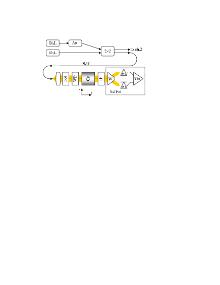
Figure 1: Schematics of one channel of the magnetometer - D₁L pump laser, D₂L probe laser. The magnetometer sensor (Cs cell) is illuminated by the two fiber coupled (polarization maintaining fibres PMF) radiations mixed (at a ratio of $50\%$) in the $2\times 2$ coupler. Before being mixed, the probe laser is attenuated down to $\mu$W level, while the pump is left at the mW level. After the Cs cell, the pump radiation is stopped by means of an interferential filter (IF), and a balanced polarimeter (BalPol), made of a Wollaston prism (W) and two photo-diodes (PD), measures the rotation of the probe beam polarization plane. The sample is positioned in the proximity of the sensor as depicted in Fig. 2

Each beam crossing the vapor is monitored by a balanced polarimeter. The Cs cells contain $23\leavevmode\nobreak\$torr of N₂ as a buffer gas. The Cs density is increased by warming it up to about 45 ^∘C using an alternating current heater supplied at $50$ kHz, a frequency higher than the atomic Larmor frequency.

After interacting with the atomic vapour, the pump radiation (about 1 mW of power) is blocked by an interference filter (IF), while the probe beam polarization is analyzed by a balanced polarimeter (BalPol). A trans-impedance amplifier (TIA) converts the photo-current into a voltage signal, which is then digitized by means of a 16 bit data acquisition (DAQ) card. The signal recorded is regarded as the real part of an analytic signal whose imaginary part is inferred by means of a numeric Hilbert transform. The total phase $\theta(t)=\omega_{0}t+\varphi$ of that analytic signal (which corresponds to the Larmor precession angle) is analysed with a linear regression routine. The phase $\varphi$ is weakly dependent upon time ($\dot{\varphi}\ll\omega_{0}$) and reproduces the Faraday rotation associated with the local time-dependent magnetic field experienced by the weak and linearly polarized probe beam.

The pump radiation is generated by a single-mode pigtailed distributed feedback diode laser, whose optical frequency is controlled via the junction current, and is periodically (synchronously with the Larmor precession) made resonant to the transition $|^{2}S_{1/2},F_{g}=3\rangle\rightarrow|^{2}P_{1/2}\rangle$ of Cs, at 894 nm.

Since the early 60’s the synchronous optical pumping has been applied to drive precessing spins bell_prl_61 . In the present work in order to achieve maximum sensitivity, both the $D_{1}L$ detuning and the modulation signal parameters have to be optimized. Due to the dual role of this radiation (hyperfine pumping and synchronous Zeeman pumping), the sensitivity depends non-trivially on these features, and this makes the optimization procedure not straightforward.

The probe laser is a single-mode Fabry-Perot, pigtailed diode, whose light is resonant with the D₂ line of Cs at 852 nm. Its radiation probes the precession state at a low rate, being $2$ GHz blue-detuned from the maximum of the triplet $|^{2}S_{1/2},F_{g}=4\rangle\rightarrow|^{2}P_{3/2}\rangle$.

The arms of the magnetometer have a base-line of $5.6\leavevmode\nobreak\ \mbox{cm}$ (making it sensitive to the field variation along the $z$ direction). The magnetometer resonance line has a linewidth of the order of  20 Hz (limited by several relaxation processes, dominated by the spin-exchange collisions) and ensures a sensitivity of $100\leavevmode\nobreak\ \mbox{fT}/\sqrt{\mbox{Hz}}$. Operating in an unshielded environment and in a gradiometric configuration the maximum sensitivity is reached at about 100 Hz, where the environmental magnetic noise is weaker and thus also the gradient/differential one gets lower. The increase in the noise at lower frequencies sets a sensitivity limit of a few pT/$\sqrt{\mbox{Hz}}$ at 1 Hz.

The magnetometer operates in a bias magnetic field ranging from $100\leavevmode\nobreak\ \mbox{nT}$ to $6\leavevmode\nobreak\ \mu\mbox{T}$, whose direction ($z$, transverse to the laser beams) is established by three pairs of square Helmholtz coils with sides of 1.8 m (see Refs.belfi_josab_07 ; belfi_rsi_10 for additional details). The magnetic field Jacobian, $G_{ij}=\partial B_{i}/\partial x_{j}$, is zeroed using five quadrupole magnets. One of the channels is used as a reference for the phase locking loop (PLL) developed to decrease the common noise in the direction of the bias field (see Ref.belfi_rsi_10 ). The PLL locking loop has a bandwidth of the order of 200 Hz.

III NMR spectroscopy experimental set-up

The experimental set-up for nuclear spin polarization, transport and manipulation is represented in Fig.2.

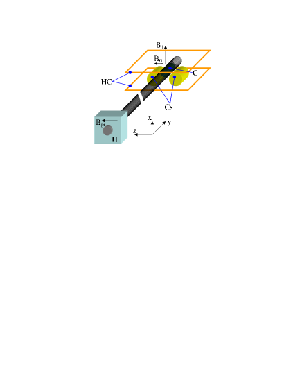
Figure 2: Sample magnetization, shuttle and positioning. The sample is contained in a polymer cartridge (C), which is inserted in a Halbach array (H) and then pneumatically shuttled into the measurement region, 2 m away. Secondary 50 cm Helmholtz coils (HC) provide transverse $B_{1}$ pulses for nuclear spin manipulation.

The sample to be analyzed, held in a 5 cm³ cartridge (3 cm in length), is initially placed in a pre-polarizing magnetic field. This pre-polarization device is based on Nd permanent magnets arranged in a Halbach array, and provides a 1 T magnetic field in a cylindrical volume of 25 mm in diameter and 50 mm in length. The sample is pre-polarized for as long as about 5 times the relaxation time measured. Subsequently it is shuttled into the proximity of the magnetometer head. A detailed description of the Halbach assembly and the pneumatic sample-shuttle is given in Ref.biancalana_rsi_14 . The travel time is of the order of 130 msec. The appropriate position of the sample with respect to the sensor cells depends on whether the longitudinal relaxation or precession signal need to be measured biancalana_jmr_09 . For the results presented in this paper the sample positioning is optimized for maximal precession signal measurement.

The measurements are performed using an automated cycle procedure, whose timing is sketched in Fig. 3.

Figure 3: Timing of the cycle for NMR spectroscopy (BT = $90$ ms; TT = $40$ ms; RT = $10-20$ ms; MT = $1-2$ s). The time interval in which the pneumatic shuttle pushes the sample towards the magnetometer head is called blowing time (BT).

The magnetic field along the sample displacement path is such that the nuclear magnetization follows it adiabatically. The exact positioning of the sample with respect to the dual channel magnetometer is verified shot by shot, and bad shots are automatically disregarded.

Operating in a low precession field makes it possible to manipulate nuclear spins by sudden field change. In our experiment, a non adiabatic (square) $B_{1}$ pulse in the $x$ direction is used to tip the nuclear spins in the $yz$ plane. The $B_{1}$ pulse is triggered by the software controlling the shuttle and DAQ operation, and is applied to a smaller Helmholtz pair (50 cm side), see Fig. 2. This produces a transverse magnetic field exceeding the bias field, which drives a rotation of the sample polarization at an angle adjustable via the pulse duration and amplitude. After being tipped with respect to the $z$ direction, nuclear spins precess around the same $B_{0}$ field where the atomic spins of the sensors are also precessing. The smaller gyromagnetic factor of the nuclei makes the nuclear signal appear to be quasi static with respect to the atomic precession.

The $B_{1}$ pulse perturbs the magnetometer, which then requires $10-30$ ms to recover its state of steady operation. Thus the pulse duration, summed with the recovery time and the sample transfer time, constitutes the total dead time after which data acquisition may start. The NMR signals presented in this paper are average signals over multiple shots, whose superposition requires accurate DAQ triggering with respect to the $B_{1}$ pulse.

The traces selected are averaged and analysed with FFT-based evaluation of their power spectral density. The data reported in this paper refer to water and to trimethyl-phosphate (${\mbox{[}CH_{3}O]_{3}PO}$) molecules, revealing in both cases only protons. This material is chosen as a test sample due to the presence of two kinds of spin-$1/2$ nuclei, one of which has a single nucleus per molecule, which simplifies appelt_pra_10 the task of developing an analytical model.

In the theoretical treatment, operating at intermediate field strengths renders several assumptions commonly used in conventional NMR spectroscopy inapplicable. A suitable model is derived here following an approach briefly described in the next section.

IV Model

We assume that the nine equivalent protons and the phosphorus nucleus can be represented as spin-$1/2$ nuclei subjected to J-coupling in an external magnetic field. To be more precise, we consider a Hamiltonian of the form ($\hbar=1$)

$$H=-\gamma_{S}\,B\,S_{z}-\gamma_{I}\,B\,I_{z}+J\operatorname{{\displaystyle\mathbf{S}\cdot\mathbf{I}}},$$ (1)

where

$$\operatorname{{\displaystyle\mathbf{S}}}=\sum_{i=1}^{9}\mathbf{s}_{i}$$ (2)

is the total spin of the protons, while $\operatorname{{\displaystyle\mathbf{I}}}$ is the spin-$1/2$ nuclei of the phosphorus. The axes are chosen in such a way that the magnetic field $B$ is in the $z$ direction. The $J$ is the exchange coupling constant ($J=\leavevmode\nobreak\ ^{3}J[H,P]$ in the experiment considered) and the $\gamma_{i}$ are the gyromagnetic constants. We also define the Larmor frequency of the two species as $\omega_{S}=\gamma_{S}B$ and $\omega_{I}=\gamma_{I}B$. The Hamiltonian (1) can almost be solved analytically bernarding_jacs_06 ; appelt_pra_10 ; abragam_61 . In fact there are 3 constants of motion which commute with $H$, namely $F_{z}=S_{z}+I_{z}$, $\operatorname{{\displaystyle\mathbf{S}}}^{2}$ and $\operatorname{{\displaystyle\mathbf{I}}}^{2}$, resulting in two useful selection rules $\Delta F_{z}=0$ and $\Delta S=0$, while $\Delta I=0$ is trivial.

The simplest basis for the state vectors of the S-type spins can be chosen as

$$|\psi\rangle=|s_{1,z}\rangle\cdots|s_{9,z}\rangle\qquad s_{i,z}=\pm 1/2$$ (3)

however, only the action of $S_{z}$ is readily written in that basis. A better choice is advisable, and, in fact, the basis states can be better labelled as

$$|\psi\rangle=|\eta;S,S_{z}\rangle,$$ (4)

where $S(S+1)$, as usual, is the eigenvalue of $\operatorname{{\displaystyle\mathbf{S}}}^{2}$, $S_{z}$ is the magnetic quantum number, and $\eta$ is a label needed to distinguish states with the same $S$ and $S_{z}$. Upon inspection one finds that there are 42 $S=1/2$, 48 $S=3/2$, 27 $S=5/2$, 8 $S=7/2$ and one $S=9/2$ states, for a total of $512=2^{9}$. Including the $\operatorname{{\displaystyle\mathbf{I}}}$ part the states are $2\times 512=1024=2^{10}$ as can be noticed in the basis (3).

The labelling of the global states is similar. Let us define

$$|\psi_{-}(M;\eta S)\rangle = |\eta S;S_{z}=M-1/2;I_{z}=1/2\rangle$$ (5)

$$|\psi_{+}(M;\eta S)\rangle = |\eta S;S_{z}=M+1/2;I_{z}=-1/2\rangle.$$ (6)

These states are eigenstates of $\operatorname{{\displaystyle\mathbf{S}}}$, $S_{z}$ and $I_{z}$ and $F_{z}=|\psi_{\pm}(M;\eta S)\rangle=M|\psi_{\pm}(M;\eta S)\rangle$.

The label $\eta$ is not present in the Hamiltonian and thus the action of $H$ on $|\psi_{\pm}(M;\eta S\rangle$ cannot depend on it abragam_61 and the matrix elements are independent of $\eta$. This is a consequence of the high symmetry of the system, which leads to a Hamiltonian depending only on the total spin operators.

The action of $H$ on these states is straightforward

$$H|\psi_{-}(M;\eta S)\rangle = a_{-}|\psi_{-}(M;\eta S)\rangle+b|\psi_{+}(M;\eta S)\rangle$$ (7)

$$H|\psi_{+}(M;\eta S)\rangle = a_{+}|\psi_{+}(M;\eta S)\rangle+b|\psi_{-}(M;\eta S)\rangle,$$ (8)

where

$$a_{\mp}=-M\omega_{S}\pm(MJ+\omega_{S}-\omega_{I})/2-J/4,$$ (9)

and

$$b=\frac{J}{2}\sqrt{S(S+1)-M^{2}-1/4}.$$ (10)

It follows that we have to diagonalize many small matrices not larger than a $2\times 2$ matrix. Consider, for instance, the states with $S_{z}=S$ so that $M=S+1/2$, we have that $|\psi_{-}(S+1/2,S)\rangle$ is an eigenstate because $|\psi_{+}(S+1/2,S)\rangle=0$ with energy $E_{-}^{e}(S)=-\omega_{S}S-\omega_{I}/2+JS/2$. Also when $S_{z}=-S$ ($M=-S-1/2$), $|\psi_{+}(-S-1/2,S)\rangle$ is an eigenstate because $|\psi_{-}(-S-1/2,S)\rangle=0$ with energy $E_{+}^{e}(-S-1/2,S)=\omega_{S}S+\omega_{I}/2+JS/2$.

The other “non extremal” states $\{|\psi_{-}(M,S)\rangle,|\psi_{+}(M,S)\rangle\}M=-(S-1/2),\ldots,S-1/2$ are coupled together and the energies read $E_{\pm}(S,M)=-(M\omega_{S}+J/4)\pm R/2$, where $R=\sqrt{(\omega_{S}-\omega_{I}+MJ)^{2}+J^{2}(S(S+1)-M^{2}+1/4)}$. Using the associated eigenstates and standard methods, we calculate the spectrum

$$\langle S_{+}(t)\rangle=\mathrm{Tr}(\rho(t)S_{+})=\mathrm{Tr}(\operatorname{{\displaystyle e}}^{-iHt}\rho(0)\operatorname{{\displaystyle e}}^{iHt}S_{+})$$ (11)

as well as $\langle I_{+}(t)\rangle$, and thus the experimental one as the real part of $\gamma_{S}\langle S_{+}(t)\rangle+\gamma_{I}\langle I_{+}(t)\rangle$.

The initial density matrix is obtained in two steps, following the experimental procedure outlined above. First the sample is polarized in a large field

$$H_{POLAR}=-\gamma_{S}B_{P}S_{z}-\gamma_{I}B_{P}I_{z}=-\bar{\omega}_{S}S_{z}-\bar{\omega}_{I}I_{z},$$ (12)

where $B_{P}=1$ T and it is justifiable to neglect the J coupling. After some time in the polarization region the density matrix of the sample reaches the thermodynamic equilibrium value

$$\begin{split}\bar{\rho}(0)&=\frac{\operatorname{{\displaystyle e}}^{-\beta H_{POLAR}}}{Z}\approx Z^{-1}(\mathbbm{1}-\beta\,H_{POLAR})\\ &=\mathbbm{1}+\beta\bar{\omega}_{S}\,S_{z}+\beta\bar{\omega}_{I}\,I_{z},\end{split}$$ (13)

where $\beta=1/(k_{B}T)$ is the inverse temperature and we drop the normalization factor $Z$ because it is just a scale factor in the spectrum as can be seen from (11).

In the second step, which takes places in the measuring region, the spins are exposed for a time $t$ to a “rotation” field $B_{1}$ as well as to the bias field $B_{0}$. Thus, neglecting the J-coupling effects, they sense the Hamiltonian

$$\begin{split}H_{R}&=-\gamma_{S}(B_{1}S_{x}+B_{0}S_{z})-\gamma_{I}(B_{1}I_{x}+B_{0}I_{z})\\ &=-(\omega_{S,R}S_{x}+\omega_{S,0}S_{z})-(\omega_{I,R}I_{x}+\omega_{I,0}I_{z})\end{split}$$ (14)

and the final density matrix is

$$\rho(0)=\operatorname{{\displaystyle e}}^{-iH_{R}t}\bar{\rho}(0)\operatorname{{\displaystyle e}}^{iH_{R}t}.$$ (15)

Defining $\Omega_{S}=\sqrt{\omega_{S,R}^{2}+\omega_{S,0}^{2}}$, $\cos\chi_{S}=\omega_{S,R}/\Omega_{S}$ and $\sin\chi_{S}=\omega_{S,0}/\Omega_{S}$ the transformed $S_{z}$ can be written as

$$\begin{split}\operatorname{{\displaystyle e}}^{-iH_{R}t}S_{z}\operatorname{{\displaystyle e}}^{iH_{R}t}=&(1-\cos(\Omega_{S}t))\sin\chi_{S}\cos\chi_{S}\;S_{x}\\ &+\cos\chi_{S}\sin(\Omega_{S}t)\;S_{y}\\ &+(\cos(\Omega_{S}t)\cos^{2}\chi_{S}+\sin^{2}\chi_{S})\;S_{z}.\end{split}$$ (16)

Using this expression and a similar one for $\operatorname{{\displaystyle e}}^{-iH_{R}t}I_{z}\operatorname{{\displaystyle e}}^{iH_{R}t}$, the explicit form of $\rho(0)$ is recovered.

The model reproduces the trimethyl-phosphate spectrum, which is reported in Fig. 4 over a wide range of magnetic fields (3 decades, from the near-zero up to the geomagnetic level). In this figure the trivial linear slope of the frequency dependence on the magnetic field is removed, i.e. the frequency axis reports the detuning from the linear $\gamma_{s}B$ value, in order to better visualize the region of interest. The spectrum contains a large set of discrete peaks at the differences of many couples selected among 1024 eigenvalues, with possible degeneracies. The selection rules reduce the total amount of transitions to 100 appelt_pra_10 ). The smooth curves reported here are obtained by convolution of such discrete spectra with a Lorentzian profile.

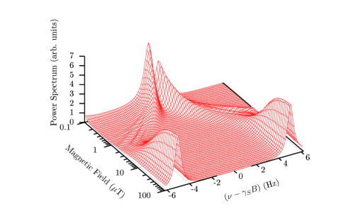
Figure 4: Simulated spectrum of trimethyl-phosphate as a function of the magnetic field, evaluated for ${}^{3}J[H,P]=63$ rad/s. For convenience, the frequency axis reports the detuning from $\gamma_{s}B$. The curve is obtained by convolving the calculated stick spectrum (made of 100 components) with a Lorentian profile. Going towards lower fields, the high-field doublet evolves in broader structures, which eventually start merging in a narrow structure at zero field. Notice that the plot reproduces only the part of the spectrum showing the evolution of the hydrogen doublet. The small increase visible in the leftmost corner at vanishing field is due to other peaks.

Figure 4 shows the well-known high-field doublet-like spectrum at magnetic fields of about 100 $\mu$T and larger, with a field-independent separation of the two peaks (the ${}^{3}J[H,P]/h$ value). In the intermediate field range (from tens of $\mu$T down to hundreds of nT) both hetero-nuclear spins and spin-field coupling determine a complex (and thus lower line intensity) spectrum with a field-dependent doublet. Here the peak separation is smaller at weaker fields. In this range, at the lower field intensity the complex spectral structures start to be resolved, rendering the doublet structure progressively less recognizable. Eventually, when approaching the near-zero-field regime, all the lines start to merge into a narrow structure, and another component starts appearing at near zero field. Only the tail of this second feature is visible in Fig. 4, where it appears as a faint increase in the leftmost corner.

V NMR spectroscopy in trimethyl-phosphate

Preliminary tests of the whole experimental setup are performed by acquiring proton signal from water samples. This step also helps to refine the calibration of the $B_{1}$ coils and to adjust the time sequences. As an example, Fig. 5 shows a precession signal from a 3.5 ml water sample both in the frequency (as power spectral density) and in the time domain. The time-domain plot is band-pass filtered to reduce the low-frequency noise and other peaks of technical noises. Working in the nT-$\mu$T range the magnetometer provides proton spectral NMR resolution better than 0.1 Hz due to magnetic field homogeneity - better than B/$\Delta$B=$10^{3}$ (at $1$ $\mu$T bias field) over the sample volume of $6.3\leavevmode\nobreak\ cm^{3}$. The stated magnetic field homogeneity is obtained compensating the first order dc magnetic field gradients with a simple and inexpensive shimming system made out of permanent magnets and large-area anti-Helmholtz coils. Thus spin relaxation and diffusion processes can be characterized with high level of accuracy.

Figure 5: NMR signal signal from water protons. The signal is produced by 3.5 ml demineralized water premagnetized for 5 sec and measured at 0.58 $\mu$T. This plot is obtained by averaging over 20 cycles. First-order bandpass filtering with cut-off frequencies at 17 and 37 Hz is applied to better visualize the time-domain trace.

The scalar coupling of the heteronuclear spin system as a function of the magnetic field is measured in a sample of trimethyl-phosphate. One example of the precession signal obtained at 4.47 $\mu$T is shown in Fig. 6. At the highest field strength investigated (of the order of 5 $\mu$T), the proton Larmor frequency is of the order of 200 Hz, the high field approximation holds, and the proton spectrum appears as a doublet. The precession signal can be approximated as a decaying beat (see Fig. 6) of two spectral components, with a separation given by the ${}^{3}J[H,P]$ constant, which amounts to about 10 Hz liao_sst_09 ; liao_rsi_10 ; mcdermott_sc_02 .

Figure 6: NMR signal obtained with a 4.0 ml trimethyl-phosphate sample, in a bias magnetic field of 4.47 $\mu$T, with a prepolarization time of $3$ seconds. The signal is an average over 500 shots. The data are filtered with a first order band-pass filter with cut-off frequencies at 170 – 220 Hz.

A simplified model of the signal made of only two components, makes it possible to fit the precession signal in Fig. 6, provided that two different decay times are considered. This simplified best-fit estimation gives time constant values of 190 ms and 240 ms for the high- and low-frequency components, respectively. This difference reflects the complexity of the theoretical spectrum presented in Fig. 7

Figure 7: Simulated spectrum of trimethyl-phosphate in the intermediate field range. The same curve shown in Fig. 4 is here plotted for the field interval investigated experimentally. This more detailed view shows that, when approaching the intermediate regime, the two high-field components become broader and start slowly approaching each other. At weaker fields they evolve in two weaker groups of partially resolved lines, which keep approaching faster and faster.

where the right-hand component of the spectrum (corresponding to the high-frequency component of the experimental spectrum) shows a bigger linewidth. The theoretical curves presented in Figs. 4 and 7 are actually obtained by convolving the discrete spectrum produced by the model with a Lorentzian profile whose width is $\Gamma=1/500$ ms, so that the width in excess is definitely set by the unresolved spectral structures.

Figure 7 shows that, besides their apparent broadening due to the separation of the unresolved components that eventually appear as secondary peaks, at weaker fields the two components of the doublet evolve into two broader and weaker groups of lines, whose spectral separation progressively decreases.

Our aim is to prove that a completely unshielded optical magnetometer is a good tool for high resolution NMR spectroscopy even in this intermediate-field regime, where the richness of the ${\mbox{[}CH_{3}O]_{3}PO}$ spectrum makes the interpretation of results difficult. Figure 8 shows the experimentally measured spectrum together with the theoretical one as a function of the bias field. The small spectral component between the peaks of the doublet structure is likely due to the presence of water protons in the sample holder.

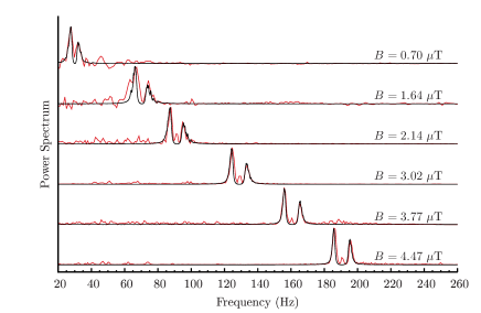
Figure 8: Trimethyl-phosphate experimental and theoretical NMR spectra recorded at different bias magnetic fields. Each trace is an average of about 500 shots. The average trace is only band-pass filtered (1-st order filter) around the doublet structure, with a cut-off frequency gap of 50 Hz.

The height of the experimental peaks is normalized, which is why a decrease of the signal-to-noise is observed at lower magnetic field. At a 700 nT bias field the overlapping of the two main structures is pronounced. A comparison between the experimental and theoretical curves is shown in Fig. 8, calculated with ${}^{3}J[H,P]=10$ Hz. There is excellent agreement between the experimental curves and the theoretical evaluation. It is worth noting that, apart from a phenomenological width of the profile used for the convolution of the discrete spectrum, the model includes only the ${}^{3}J[H,P]$ as a free parameter. Thus the close correspondence between theory and experiment demonstrates that useful information and accurate evaluations can also be inferred from measurements performed in this intermediate regime.

VI Conclusion

In this paper we report ZULF-NMR spectroscopy results obtained with a trimethyl-phosphate sample of 4 ml in volume premagnetized in a 1 T field. The experiment is based on remote-detection of precession signal in an unshielded environment by means of a differential optical magnetometer. The system is tested at intermediate field strengths, where the ${}^{3}J[H,P]$ coupling and the spin-field interaction are of the same order of magnitude. An analytical model is developed to interpret the spectra observed, obtaining consistent predictions.

The work presented here shows the potential of optical magnetometry in ZULF-NMR spectroscopy even in an unshielded environment and when operating in a disadvantageous regime, where a complex spectral structure renders signal analysis a challenging task.

References

References

- (1) M. P. Ledbetter, D. Budker, Zero-field nuclear magnetic resonance, Physics Today 66 (2013) 44–49.
- (2) D. Sheng, S. Li, N. Dural, M. V. Romalis, Subfemtotesla scalar atomic magnetometry using multipass cells, Phys. Rev. Lett. 110 (2013) 160802.
- (3) D. P. Weitekamp, A. Bielecki, D. Zax, K. Zilm, A. Pines, Zero-Field Nuclear Magnetic Resonance, Physical Review Letters 50 (1983) 1807–1810.
- (4) J. Bernarding, G. Buntkowsky, S. Macholl, S. Hartwig, M. Burghoff, and L. Trahms, J-Coupling Nuclear Magnetic Resonance Spectroscopy of Liquids in nT Fields, Journal of the American Chemical Society, (2006), 714-715
- (5) I. M. Savukov, M. V. Romalis, NMR Detection with an Atomic Magnetometer, Physical Review Letters 94 (12) (2005) 123001.
- (6) G. Bevilacqua, V. Biancalana, Y. Dancheva, L. Moi, Chapter three - optical atomic magnetometry for ultra-low-field NMR detection, Vol. 78 of Annual Reports on NMR Spectroscopy, Academic Press, 2013, Ch. 3, pp. 103 – 148.
- (7) I. Savukov, T. Karaulanov, Anatomical MRI with an atomic magnetometer, Journal of Magnetic Resonance 231 (0) (2013) 39 – 45.
- (8) S. Xu, V. V. Yashchuk, M. H. Donaldson, S. M. Rochester, D. Budker, A. Pines, Magnetic resonance imaging with an optical atomic magnetometer, Proceedings of the National Academy of Sciences 103 (34) (2006) 12668–12671.
- (9) R. McDermott, N. Kelso, S.-K. Lee, M. Mößle, M. Mück, W. Myers, B. Haken, H. Seton, A. Trabesinger, A. Pines, J. Clarke, Squid-detected magnetic resonance imaging in microtesla magnetic fields, Journal of Low Temperature Physics 135 (5-6) (2004) 793–821.
- (10) M. P. Ledbetter, I. M. Savukov, D. Budker, V. Shah, S. Knappe, J. Kitching, D. J. Michalak, S. Xu, A. Pines, Zero-field remote detection of NMR with a microfabricated atomic magnetometer, Proceedings of the National Academy of Science 105 (2008) 2286–2290.
- (11) M. C. Butler, M. P. Ledbetter, T. Theis, J. W. Blanchard, D. Budker, A. Pines, Multiplets at zero magnetic field: The geometry of zero-field NMR, Journal of Chemical Physics 138 (18) (2013) 184202.
- (12) M. P. Ledbetter, T. Theis, J. W. Blanchard, H. Ring, P. Ganssle, S. Appelt, B. Blümich, A. Pines, D. Budker, Near-Zero-Field Nuclear Magnetic Resonance, Physical Review Letters 107 (10) (2011) 107601.
- (13) S. Appelt, F. W. Häsing, H. Kühn, U. Sieling, B. Blümich, Analysis of molecular structures by homo- and hetero-nuclear J-coupled NMR in ultra-low field, Chemical Physics Letters 440 (2007) 308–312.
- (14) T. Theis, J. W. Blanchard, M. C. Butler, M. P. Ledbetter, D. Budker, A. Pines, Chemical analysis using J-coupling multiplets in zero-field NMR, Chemical Physics Letters 580 (2013) 160–165.
- (15) S. Appelt, F. W. Häsing, U. Sieling, A. Gordji-Nejad, S. Glöggler, B. Blümich, Paths from weak to strong coupling in NMR, Phys. Rev. A 81 (2010) 023420.
- (16) J. Belfi, G. Bevilacqua, V. Biancalana, S. Cartaleva, Y. Dancheva, L. Moi, Cesium coherent population trapping magnetometer for cardiosignal detection in an unshielded environment, JOSA B 24 (9) (2007) 2357–2362.
- (17) J. Belfi, G. Bevilacqua, V. Biancalana, R. Cecchi, Y. Dancheva, L. Moi, Stray magnetic field compensation with a scalar atomic magnetometer, Review of Scientific Instruments 81 (6) (2010) 065103.
- (18) A. J. Dingley, F. Cordier, S. Grzesiek, An introduction to hydrogen bond scalar couplings, Concepts in Magnetic Resonance 13 (2) (2001) 103–127.
- (19) S.-H. Liao, H.-C. Yang, H.-E. Horng, S. Y. Yang, H. H. Chen, D. W. Hwang, L.-P. Hwang, Sensitive J-coupling spectroscopy using high-Tc superconducting quantum interference devices in magnetic fields as low as microteslas, Superconductor Science Technology 22 (4) (2009) 045008.
- (20) S.-H. Liao, M.-J. Chen, H.-C. Yang, S.-Y. Lee, H.-H. Chen, H.-E. Horng, S.-Y. Yang, A study of J-coupling spectroscopy using the Earth’s field nuclear magnetic resonance inside a laboratory, Review of Scientific Instruments 81 (10) (2010) 104104.
- (21) W. Bell, A. Bloom, Optically driven spin precession, Phys. Rev. Lett., 6(6) (1961) 280.
- (22) V. Biancalana, Y. Dancheva, L. Stiaccini, Note: A fast pneumatic sample-shuttle with attenuated shocks, Review of Scientific Instruments 85 (3) (2014) 036104.
- (23) G. Bevilacqua, V. Biancalana, Y. Dancheva, L. Moi, All-optical magnetometry for NMR detection in a micro-Tesla field and unshielded environment, Journal of Magnetic Resonance 201 (2009) 222–229.
- (24) A. Abragam, Principle of Nuclear Magnetism, Clarendon University Press, Oxford, 1961.
- (25) R. McDermott, A. H. Trabesinger, M. Mück, E. L. Hahn, A. Pines, J. Clarke, Liquid-State NMR and Scalar Couplings in Microtesla Magnetic Fields, Science 295 (2002) 2247–2250.