Likelihood Ratio Tests for a Dose-Response Effect using Multiple Nonlinear Regression Models

Abstract

We consider the problem of testing for a dose-related effect based on a candidate set of (typically nonlinear) dose-response models using likelihood-ratio tests. For the considered models this reduces to assessing whether the slope parameter in these nonlinear regression models is zero or not. A technical problem is that the null distribution (when the slope is zero) depends on non-identifiable parameters, so that standard asymptotic results on the distribution of the likelihood-ratio test no longer apply. Asymptotic solutions for this problem have been extensively discussed in the literature. The resulting approximations however are not of simple form and require simulation to calculate the asymptotic distribution. In addition their appropriateness might be doubtful for the case of a small sample size. Direct simulation to approximate the null distribution is numerically unstable due to the non identifiability of some parameters. In this article we derive a numerical algorithm to approximate the exact distribution of the likelihood-ratio test under multiple models for normally distributed data. The algorithm uses methods from differential geometry and can be used to evaluate the distribution under the null hypothesis, but also allows for power and sample size calculations. We compare the proposed testing approach to the MCP-Mod methodology and alternative methods for testing for a dose-related trend in a dose-finding example data set and simulations.

1 Introduction

A major objective in the development of a pharmaceutical compound is the characterisation of its dose-response curve. For this purpose Phase II trials are conducted that compare several doses of the compound to placebo. Then (typically) nonlinear regression models are used to estimate the underlying dose-response curve. See for example Bretz et al. (2005); Thomas (2006); Dragalin et al. (2007); Jones et al. (2011) or Grieve and Krams (2005) for different approaches towards model-based dose-response analyses in Phase II studies.

Typically the model linking dose and response can be assumed to follow a nonlinear function of the form $\alpha+\beta x_{\text{}}$, where $\alpha$ and $\beta$ are linear parameters describing the placebo response and the slope parameter, and $x_{\text{}}$ is a nonlinear transformation of the dose variable $z$ depending on a parameter vector . The major question regarding the dose-response curve that we will consider in this article is to assess whether there exists a dose-related effect (i.e. a dose-response trend) or not. For the dose-response function above this reduces to testing the hypothesis of $\beta=0$.

One of the challenges with a dose-response model based approach is that there is model uncertainty at the design stage of the trial, when the statistical analyses are specified. That means specifying one particular form of the dose-response curve bears the risk of mis-specification. Naively one might think that it is valid to apply a model selection procedure to obtain the best model once one has obtained the data and then perform a test for a dose-related effect, ignoring the fact that a model selection was performed. However it is known that statistical inference following a model selection is no longer valid in the sense of not providing confidence intervals of nominal coverage and resulting in a type I error inflation (Chatfield (1995); Leeb and Pötscher (2005), or Chapter 7 of Claeskens and Hjort (2008)). These concerns might have lead to a situation where primarily ANOVA type methods have been used in Phase II trials, which do not assume a functional relationship between dose and response. This, however, comes at a loss in terms of statistical efficiency but also interpretability of the study results.

A compromise between approaches that make no assumptions on the functional form of the dose-response curve and those that assume one specific dose-response model is to specify a candidate set of dose-response models. This is the idea underlying the Multiple Comparison Procedures and Modeling (MCP-Mod) approach (Bretz et al. (2005); Pinheiro et al. (2014); European Medicines Agency (2014)). MCP-Mod consists of two steps: testing and estimation. The testing step, which is of primary interest for this article, is done using multiple linear contrast tests. To derive contrast tests that are powerful to detect the nonlinear shapes in the candidate set, one needs to pre-specify the parameters of the nonlinear part of the regression functions. This approach bears the risk of model mis-specification (as a different from the one pre-specified might be adequate).

An alternative approach is to assess the hypothesis $\beta=0$ by using multiple likelihood-ratio tests. Arguments by Andrews and Ploberger (1995) and Andrews (1996) show that the likelihood-ratio test will always be admissible in this setting (i.e., there is no test that controls the type-I error and is uniformly more powerful). A technical problem with such likelihood-ratio tests is that under the null hypothesis the parameters of the nonlinear regression models are asymptotically not identifiable. Therefore, the standard asymptotic results for the null distribution of likelihood-ratio statistics do no longer apply; see for example Davies (1977), Davies (1987), Andrews and Ploberger (1994), Ritz and Skovgaard (2005) and Liu and Shao (2003). Dette et al. (2015) derive the asymptotic null distribution of the likelihood-ratio statistic under multiple models. Baayen et al. (2015) only consider nested dose-response models, but describe a similar approach, where the asymptotic distribution for the likelihood-ratio tests is derived explicitly. The resulting asymptotic distribution is not of a simple form and requires simulation to approximate critical values and p-values that are asymptotically valid.

We will consider the exact distribution for likelihood-ratio tests for the null hypothesis that no trend exists against the composite alternative that one of the candidate models is true. We assume that observations are independent and normally distributed and that the dose-response models are piece-wise continuous, which is generally true for the models considered in practice.

To find the small-sample distribution of the likelihood-ratio statistic, one can of course simulate data and fit the dose-response models under the null hypothesis ($\beta=0$) to obtain critical values for the test statistic. However, as most of the statistical models considered in this article are nonlinear, computationally expensive iterative techniques are required to calculate the maximum likelihood estimates for each model and each simulated data set. Such an approach is also numerically unstable under $\beta=0$ as the likelihood function will be almost flat with potentially several local maxima for the non-identifiable parameter .

In this article, we work with the small-sample distribution of the likelihood-ratio statistic using methods developed by Hotelling (1939) and Weyl (1939) and reviewed from a statistical perspective by Johansen and Johnstone (1990). We start with the special case of a single model. For this special case, Hotelling used a geometric approach to derive the exact null distributions analytically. We extend these methods to multiple dose-response models and show that, as in the case of a single model, the distribution is determined by volumes of certain tubular neighborhoods on the unit sphere. We then present an importance sampling-type algorithm to approximate such volumes numerically. In particular, this approach does not require the calculation of maximum-likelihood estimates (with its associated numerical difficulties) in each simulation run. Using this approach, it is also possible to evaluate the power of the proposed test under alternative hypotheses, thereby enabling sample-size calculations, which are crucial in clinical development.

The outline of this paper is as follows. After introducing the notation in Section 2.1, we will review the application of Hotelling's approach for the case of one dose-response model in Section 2.2.2. We then present the new methodology in Section 2.2.4 and Section 2.3, where a numerical algorithm is introduced to approximate the distribution of the likelihood-ratio test. In Section 3 we apply the method to data from a dose-response study and compare the performance of the new method to MCP-Mod and a number of alternative approaches in a setting motivated by this example data. Section 4 gives some concluding remarks.

2 Methods

2.1 Notation

Consider a random vector $y$ containing the clinical measurement of interest for each of the $n$ patients. Here we assume $y\sim\mathcal{N}(\mu,\sigma^{2}I_{n})$ with $n$ independent, normally distributed observations with an unknown common standard deviation $\sigma\in\mathbb{R}_{+}$ and an unknown mean vector $\mu\in\mathbb{R}^{n}$.

To describe possible forms of the mean vector $\mu$, one selects $m$ candidate dose-response models of the following partially-linear form

$$\mu_{i}(\alpha,\beta,\text{})=\alpha\mathbf{1}_{n}+\beta\,x_{\text{},i}\quad(\alpha,\beta\in\mathbb{R},\;\text{}\in\Gamma_{i},\;i=1,\dots,m)$$ (1)

where $x_{\text{},i}=x_{\text{},i}(z)$ are nonlinear transformations of the dose variable $z$. Since the value of $z$ can be fixed throughout, the dependencies on $z$ will not be explicitly indicated. We assume that the nonlinear transformations $\text{}\mapsto x_{\text{},i}:\Gamma_{i}\to\mathbb{R}^{n}$ are piece-wise-continuous functions. One example is the so-called Emax model

$$\mu_{i}(\alpha,\beta,\text{})=\alpha+\beta x_{\text{}},\qquad x_{\text{}}=z/(z+\text{}),\qquad\alpha,\beta\in\mathbb{R},\;\text{}\in\Gamma=\mathbb{R}_{+};$$

for more examples, see, e.g.,  Bornkamp et al. (2009).

Note that for $\beta=0$, the value of in (1) has no influence on the shape of the model function, which means that asymptotically the parameter is not identified.

We will consider the hypothesis $\mu\in H_{0}$, where

$$H_{0}=\{\alpha\mathbf{1}_{n}:\alpha\in\mathbb{R}\},$$ (2)

the one-sided alternatives $\mu\in H_{1},\dots,\mu\in H_{2m}$, where, for $i=1,\dots,m$,

$$H_{i}=\{\mu_{i}(\alpha,\beta,\text{}):\alpha\in\mathbb{R},\beta\in\mathbb{R}_{+},\text{}\in\Gamma_{i}\},$$ (3)

$$H_{m+i}=\{\mu_{i}(\alpha,-\beta,\text{}):\alpha\in\mathbb{R},\beta\in\mathbb{R}_{+},\text{}\in\Gamma_{i}\},$$ (4)

and the multiple alternatives $\mu\in H_{I}$, where

$$H_{I}=\bigcup_{i\in I}H_{i},\quad\text{for}~{}I\subseteq\{1,\dots,2m\}.$$ (5)

For the special cases $I=\{1,\dots,m\}$ or $I=\{m+1,\dots,2m\}$ we get one-sided alternatives, and for the special case $I=\{1,\dots,2m\}$ a two-sided alternative. The goal will be to derive the likelihood-ratio test for $H_{0}$ against $H_{I}$.

2.2 Distribution of the LR test

To illustrate the general approach for calculation of the distribution of the likelihood-ratio test we will start with the simple setting of a single linear dose-response model first in Section 2.2.1, then consider a single nonlinear model in Section 2.2.2 and finally present the situation for multiple dose-response models in Section 2.2.4.

2.2.1 Single linear dose-response model

We first consider the special case of testing $H_{0}$ against a single hypothesis $H_{i}$ (so that $I=\{i\}$), where $\Gamma_{i}=\{\text{}_{i}\}$ contains a single parameter value $\text{}_{i}$. In this case $\text{}_{i}$ is known and the dose-response model reduces to a linear regression model. If we define $x=x_{\text{}_{i},i}$, then $H_{i}$ becomes the hypothesis $\beta>0$ in the linear model $y\sim\mathcal{N}(\alpha\mathbf{1}_{n}+\beta x,\;\sigma^{2}I_{n})$, while $H_{0}$ states that $\beta=0$. In this case standard distributional results can be used to calculate the distribution of the LR test statistic for testing $\beta=0$. The reason, why we present this case here is to motivate a transformation of the standard LR test statistic that turns out to be useful for subsequent sections.

Appendix A shows that the LR statistic has the form $S(R)=(1-\mathbbm{1}{\{R>0\}}R^{2})^{n/2}$ with

$$R=\tilde{x}^{\top}\tilde{y},\qquad\text{where}\quad\tilde{x}=\frac{Bx}{\lVert Bx\rVert}\quad\text{and}\quad\tilde{y}=\frac{By}{\lVert By\rVert},$$ (6)

where the rows of the $(n-1)\times n$ matrix $B$ form an orthonormal basis for the linear subspace $\mathbb{L}=\{a\in\mathbb{R}^{n}:a^{\top}1_{n}=0\}$ and $\lVert\cdot\rVert$ denotes the Euclidean norm. The LR test rejects $H_{0}$ if $S$ is small enough, or equivalently, since $S$ is non-increasing in $R$, if $R$ is large enough.

The model predicts that the mean vector has the form $\alpha\mathbf{1}_{n}+\beta x$, so that the centered and scaled prediction from the model equals $B(\alpha 1_{n}+\beta x)/\lVert B(\alpha 1_{n}+\beta x)\rVert=(Bx)/\lVert Bx\rVert=\tilde{x}$ in the basis $B$. Furthermore, $\tilde{y}$ contains the standardized (centered and scaled) observations, so that both $\tilde{x}$ and $\tilde{y}$ lie on the unit sphere. The centering and scaling implies that $R$ is the correlation coefficient between observations and predictions and $R^{2}$ the coefficient of determination (Seber and Lee, 2003, Section 4.4). Since the inner product between the two unit vectors $\tilde{x}$ and $\tilde{y}$ increases monotonically with the distance between the two vectors, the LR test rejects $H_{0}$ if the standardized predictions are close enough to the standardized observations.

Let $d=n-2$ denote the degrees of freedoms and $\mathbb{S}=\{s\in\mathbb{R}^{d+1}:\lVert s\rVert=1\}$ the $d$-dimensional unit sphere (some authors call it the $d+1$ dimensional unit sphere since it is in $\mathbb{R}^{d+1}$). Then $\tilde{x}\in\mathbb{S}$ and $\tilde{y}$ is uniformly distributed on $\mathbb{S}$ under $H_{0}$, which can be seen as following: the assumption of $H_{0}$ is $y\sim\mathcal{N}(\alpha\mathbf{1}_{d+2},\sigma^{2}I_{d+2})$; hence $By\sim\mathcal{N}(\alpha B\mathbf{1}_{d+2},\sigma^{2}BB^{\top})$ with $\alpha B\mathbf{1}_{d+2}=\mathbf{0}_{d+1}$ (since $\mathbf{1}_{d+2}$ is orthogonal to $\mathbb{L}$) and $BB^{\top}=I_{d+1}$; hence $By$ is spherically symmetric (Fang and Zhang, 1990) and $\tilde{y}$ is uniformly distributed on $\mathbb{S}$.

The p-value of the LR test is $P_{0}(R>r)$, with $r$ for the observed value of $R$ and $P_{0}(\cdot)$ the probability calculated under the null hypothesis $H_{0}$ (since the distribution of $R$ does not depend on the parameter $\alpha$, we may assume $\mu=\mathbf{0}_{n}$ for $P_{0}$). If we define the neighborhood around a point $s\in\mathbb{S}$ (a spherical cap) as $\mathbb{C}_{sr}=\{t\in\mathbb{S}:s^{\top}t>r\}$, then $P_{0}(R>r)$ is equal to the probability that $\tilde{y}$ is in the spherical cap around $\tilde{x}$ defined by $r$ under $H_{0}$: $P_{0}(R>r)=P_{0}(\tilde{y}\in\mathbb{C}_{\tilde{x}r})$; see Figure 1. As $\tilde{y}$ is uniformly distributed on $\mathbb{S}$ under $H_{0}$ it follows that $P_{0}(\tilde{y}\in\mathbb{C}_{\tilde{x}r})=\left\lvert\mathbb{C}_{\tilde{x}r}\right\rvert/\left\lvert\mathbb{S}\right\rvert$ where $\left\lvert\cdot\right\rvert$ is the ($d$-dimensional) volume of a set on $\mathbb{S}$. Since the volume of the spherical cap $\left\lvert\mathbb{C}_{sr}\right\rvert$ does not depend on the point $s\in\mathbb{S}$, we will simply write $\left\lvert\mathbb{C}_{r}\right\rvert$ for such a volume.

Using the equations for the volumes of spheres and of spherical caps (Li, 2011), we get

$$P_{0}(R>r)=\frac{\left\lvert\mathbb{C}_{r}\right\rvert}{\left\lvert\mathbb{S}\right\rvert}=\frac{1-F(r^{2},1/2,d/2)}{2},\qquad\text{for $r\in[0,1]$},$$ (7)

where $F(\cdot,a,b)$ denotes the cdf of the beta distribution with parameters $a,b\in\mathbb{R}_{+}$. The equation when $r\in[-1,0)$ follows from $\left\lvert\mathbb{C}_{r}\right\rvert=\left\lvert\mathbb{S}\right\rvert-\left\lvert\mathbb{C}_{-r}\right\rvert$.

.

Figure 1: Standardized prediction $\tilde{x}$, standardized observation $\tilde{y}$, and spherical cap $\mathbb{C}_{\tilde{x},r}$ (gray area) when $d=1$ (left side) and when $d=2$.

Of course, in this section we have only derived a test equivalent to the standard t-test for the linear model. However, the considerations will be useful in the following sections.

2.2.2 Single nonlinear dose-response model

Figure 2: Left plot: Observed point $y$ (open circles) and the exponential curves $z\mapsto\exp(z/\text{})$, with $z\in[0,3]$ for the four values $\text{}=0.1,0.7,1.6,10$ plotted in the zero-one standardization; the curve for $\text{}=0.1$ is the lowest (most convex) curve, while the curve for $\text{}=10$ is the topmost (almost linear) curve. Middle plot: tubular neighborhood $\mathbb{T}_{r}$ (gray area) around the curve $\mathbb{M}=\{\tilde{x}_{\text{}}:\text{}\in[0.1,10]\}$ (black line) for the model $x_{\text{}}^{(k)}=\exp(z^{(k)}/\text{})$ with $z^{(k)}=k-1$ for $k=1,2,3$. Right plot: model curve for the counterexample at the end of Section 2.2.3.

We now consider again the case of a single hypothesis $I=\{i\}$, but generalize to the situation, where the parameter space $\Gamma_{i}$ no longer consists of a single point. We write $\Gamma=\Gamma_{i}$ and $x_{\text{}}=x_{\text{},i}$.

By the considerations in the last section, the LR statistic for a fixed value $\text{}\in\Gamma$ equals $R_{\text{}}=\tilde{x}_{\text{}}^{\top}\tilde{y}$, with $\tilde{x}_{\text{}}=(Bx_{\text{}})/\lVert Bx_{\text{}}\rVert$. Therefore, the LR statistic of $H_{0}$ against $H_{i}$ equals $\inf_{\text{}\in\Gamma}{S(R_{\text{}})}=S(R)$ with $R=\sup_{\text{}\in\Gamma}R_{\text{}}$ since $S$ is continuous and non-increasing in $R$.

Write again $r$ for the observed value of $R$, define the model set $\mathbb{M}=\{\tilde{x}_{\text{}}:\text{}\in\Gamma\}$ of the standardized prediction that are possible under $H_{i}$, and define the tubular neighborhood $\mathbb{T}_{r}=\mathbb{T}_{r}(\mathbb{M})=\bigcup_{s\in\mathbb{M}}\mathbb{C}_{sr}$ around $\mathbb{M}$. Then it follows from the uniform distribution of $\tilde{y}$ that

$$p=P_{0}(R>r)=P_{0}(\tilde{y}\in\mathbb{T}_{r})=\left\lvert\mathbb{T}_{r}\right\rvert/\left\lvert\mathbb{S}\right\rvert.$$

The volume $\left\lvert\mathbb{S}\right\rvert$ of the unit sphere is straightforward to calculate. Hotelling (1939) gives explicit equations for $\left\lvert\mathbb{T}_{r}\right\rvert$ when $\mathbb{M}$ is a closed curve that satisfies certain regularity conditions (essentially the nonlinear transformation $x_{\text{}}$ needs to be sufficiently smooth) . These results have been extended to more general manifolds $\mathbb{M}$; see, for example, Naiman (1990) and Gray (2004), and the references therein.

The middle plot of Figure 2 illustrate this construction for the exponential model $x_{\text{}}^{(k)}=\exp(z^{(k)}/\text{})$ with $z^{(k)}=k-1$ for $k=1,2,3$. Here and in the following, we will write $x^{(k)}$ and $z^{(k)}$ for the $k$-th elements of the vectors $x$ and $z$. Assume that we observe a point $y=(-0.6,\,-0.2,\,0,\,0.8)^{\top}$. The correlation $R_{\text{}}=\tilde{x}_{\text{}}^{\top}\tilde{y}$ is maximized when $\text{}=1.7$. Four points $\tilde{x}_{0.1},\,\tilde{x}_{0.7},\,\tilde{x}_{1.6}\,\tilde{x}_{10}$, which are equally spaced on $\mathbb{M}$, are shown together with their spherical caps; the tubular neighborhood $\mathbb{T}_{r}$ is generated by moving the spherical cap along the curve $\mathbb{M}$. Note that equal spacing of points on $\mathbb{M}$ leads to unequally parameter values , this is due to the nonlinearity of the model function.

Since $R_{\text{}}$ is invariant under affine transformations of $x_{\text{}}$ and $y$, we may scale them to the unit interval (``zero-one standardization''), as shown in the left-hand side of Figure 2.

2.2.3 $\chi^{2}$ critical values

Before we continue to the case of multiple models in the next section, we will consider what could happen if we would simply ignore the identifiability issue and would assume that the statistic $-2\log S$ is asymptotically $\chi^{2}$ distributed.

The critical value of such a test would depend only on the number of parameters in the model, but not on the area of on sphere covered by the model. One can construct an example that shows that such a test can not control the type-I error in general: in fact, for any critical value $q\in\mathbb{R}_{+}$ of the statistic $-2\log S$, there exists a model so that the resulting test always rejects (has type-I error 1). The idea is to choose the model in such way that the standardized predictions form a curve that comes arbitrarily close to any point on the unit sphere. In Appendix B we give the model equation for a model function that fulfills these requirements, see also the right-hand side of Figure 2, which gives a graphical illustration of this model.

2.2.4 Multiple nonlinear dose-response models

The case of multiple models can be treated along the lines of a single model, just by forming the union of the dose-response model shapes on the unit sphere: the multiple models can be collapsed into a single big model, so that the case of a candidate set of models is along the lines of the single model. From a multiple testing perspective a max-test is being performed, i.e. the maximum being over the different candidate dose-response models.

In more detail, the LR statistic is a monotonous function of the statistic

$$R=\max_{i\in I}\sup_{\text{}_{i}\in\Gamma_{i}}\tilde{x}_{\text{}_{i},i}^{\top}\tilde{y},\qquad\text{with}\ \tilde{x}_{\text{}_{i},i}=(Bx_{\text{}_{i},i})/\lVert Bx_{\text{}_{i},i}\rVert.$$

Equivalently, we can write $R$ as $R=\sup_{\text{}\in\Gamma^{\prime}}\tilde{x}_{\text{}}^{\top}\tilde{y}$ for a single (composite) model

$$\Gamma^{\prime}=\bigcup_{i\in I}\bigl{\{}\Gamma_{i}\times\{i\}\bigr{\}},\qquad\tilde{x}_{(\text{}_{i},i)}=\tilde{x}_{\text{}_{i},i}.$$

If we define $\mathbb{M}=\{\tilde{x}_{\text{}}:\text{}\in\Gamma^{\prime}\}$ and $\mathbb{T}_{r}(\mathbb{M})$ for this composite model, then the task reduces to the calculation of the volume $\left\lvert\mathbb{T}_{r}\right\rvert$, since

$$P_{0}(R>r)=\left\lvert\mathbb{T}_{r}\right\rvert/\left\lvert\mathbb{S}\right\rvert.$$

Analytic methods developed for the case of a single model can no longer be used as the different models might have intersecting curves on the unit-sphere (see Figure 3 for an illustration), which is why specialized numerical methods need to be developed to calculate the associated tubular volumes.

In addition to the overall p-value $p=P_{0}(R>r)$, the multiplicity-adjusted p-values $p_{i}=P_{0}(R>r_{i})$ for the individual hypothesis $H_{i}$, for $i\in I$, are also of interest, where $r_{i}$ is the correlation between the observations and the best predictions under the hypothesis $H_{i}$.

This ``multiplicity'' penalty has a direct geometric interpretation: if the candidate set of dose-response models gets larger, the standardized predictions cover larger parts on the unit sphere; consequently, the tube around the standardized model predictions has to get thinner if the volume $\left\lvert\mathbb{T}_{r}\right\rvert$ (and therefore the type-I error) should be kept constant.

Figure 3: Standardized predictions $\mathbb{M}_{i}=\{\tilde{x}_{i,\text{}_{i}}:\text{}_{i}\in\Gamma_{i}\}$ and tubular neighborhoods $\mathbb{T}_{ri}=\mathbb{T}_{r}(\mathbb{M}_{i})$ for the models $x_{1,\text{}}^{(k)}=\cos(z^{(k)}+\text{})$ and $x_{2,\text{}}^{(k)}=(z^{(k)})^{\text{}}/(z^{(k)})^{\text{}}+1.5)$, where $\Gamma_{1}=[\pi,(5/4)\pi]$ and $\Gamma_{2}=[10^{-3},5]$, when $z=(0,\dots,3)^{\top}$. Due to the overlap between the two neighborhoods, the volume of the combined tube, $\left\lvert\mathbb{T}_{r1}\cup\mathbb{T}_{r2}\right\rvert$, is smaller then the sum of the two volumes, $\left\lvert\mathbb{T}_{r1}\right\rvert+\left\lvert\mathbb{T}_{r2}\right\rvert$.

2.3 Numerical calculation of tubular volumes

This section describes an algorithm motivated by importance sampling to approximate the probabilities $P_{0}(R>r)=P_{0}(\tilde{y}\in\mathbb{T}_{r})$, to obtain p-values or a critical value $r_{crit}$ for the test statistic $R$. As discussed earlier, under the null hypothesis, $\tilde{y}$ is uniformly distributed on the sphere, so that $P_{0}(R>r)=\int_{\mathbb{T}_{r}}\mathrm{d}\varsigma$, with $\varsigma$ the uniform probability measure on $\mathbb{S}$. In addition to p-values and the critical value, we are also be interested in calculating the power $P_{1}(R>r)=P_{1}(\tilde{y}\in\mathbb{T}_{r})$, for a critical value $r$, with $P_{1}(\cdot)$ a probability calculated under some alternative hypothesis. By arguments due to Pukkila and Rao (1988), under alternative hypotheses, $\tilde{y}$ follows an angular Gaussian distribution on $\mathbb{S}$, which means that $P_{1}(R>r)=\int_{\mathbb{T}_{r}}f\,\mathrm{d}\varsigma$, where $f:\mathbb{S}\to\mathbb{R}$ is the density of the angular Gaussian density (of course, under the null-hypothesis $f\equiv 1$.)

Let us motivate the algorithm by considering a naive sampling approach. If we draw a sample $U_{1},\dots,U_{\kappa}$ uniformly from $\mathbb{S}$, then $\int_{\mathbb{T}_{r}}f\,\mathrm{d}\varsigma\approx\sum_{k=1}^{\kappa}\mathbbm{1}{\{U_{k}\in\mathbb{T}_{r}\}}f(U_{k})/\kappa$. However, since $\mathbb{T}_{r}$ is only implicitly defined by the nonlinear models, deciding if a point $U_{k}$ belongs to $\mathbb{T}_{r}$ requires the computationally expensive calculation of the maximum-likelihood estimates for each of the nonlinear models.

A better approach is to restrict sampling to $\mathbb{T}_{r}$ instead of sampling from the whole sphere $\mathbb{S}$. If one can construct a probability distribution supported only on $\mathbb{T}_{r}$ with known density $g$ with respect to $\varsigma$, and generate a sample $V_{1},\dots,V_{\kappa}$ according to this distribution, then we could use importance sampling to obtain the approximation

$$\int_{\mathbb{T}_{r}}f\,\mathrm{d}\varsigma\approx\frac{1}{\kappa}\sum_{k=1}^{\kappa}\frac{f(V_{k})}{g(V_{k})}.$$ (8)

However, calculating such density $g$ is challenging. The approach proposed in this paper is to sample points $V_{1},\dots,V_{\kappa}$ in such a way that even if we can not calculate $g$ exactly, we can approximate $g$ from the sample itself. The main idea for sampling only within $\mathbb{T}_{r}$ is to first sample a model $i$ from the $m$ models with equal probability, then sample a value from $\Gamma_{i}$ according to some convenient distribution (for example, the uniform distribution if $\Gamma_{i}$ has finite volume) and take $W=\tilde{x}_{\text{},i}$. Then one samples a point $V$ from $G_{W}$, the uniform probability distribution on the spherical cap $\mathbb{C}_{Wr}$ around $W$ with radius $r$. It is possible to approximate the density $g$ underlying this proposal sampling mechanism (see the Appendix C for details), which is needed to calculate the importance ratios in (8).

Note that in the strict sense however this is not an importance sampling algorithm, as the proposal density $g$ as well as integral are determined from the same sampled values. In Appendix C the consistency of the sampling scheme is proved. That means that the approximation error of the algorithm can be made arbitrarily small by increasing the number of sampling replicates $\kappa$. The number of simulations can be chosen by monitoring the Monte Carlo standard error, to obtain the desired precision.

2.4 Comparison to MCP-Mod

The multiple contrast test of the MCP-Mod procedure  (Bretz et al., 2005) can be viewed as a discrete analogue of the likelihood-ratio approach presented here, as each model is restricted to a finite number of possible shapes in MCP-Mod.

Even in the case of a finite number of possible shapes (when both approaches are applicable), the likelihood-ratio test seems preferable due to the following argument. The t-test for testing $\beta=0$ is uniformly most powerful invariant with respect to affine transformations (Lehmann and Romano, 2008, Chapter 7). While the likelihood-ratio test is equivalent to the t-test, the corresponding contrast test statistic is invariant but differs from the t-test in the variance estimate; hence it is not in general admissible (although in this setting power gains by an LR test are unlikely to be large).

3 Applications

In this section we will use data from a dose-response clinical trial to illustrate the methodology. One of the objectives of such trials is to test for a dose-response effect, that is, whether the dose-response is flat or not. Motivated by the data, we define some scenarios and compare the approach to alternative trend tests: Section 3.2 considers a single candidate model; Section 3.3 considers a candidate set of models.

In all examples considered p-values and power values were calculated using a Monte Carlo standard error of at most $0.001$, or when a maximum sample of $10^{6}$ samples was reached in the algorithm. Calculation of the critical value was done using root-findung under the null-hypothesis.

3.1 Dose-Finding Example

The purpose of this section is to illustrate the methodology on a real data set and compare it to the MCP-Mod methodology. The section also illustrates how the critical value (and thus the multiplicity adjustment) depends on the complexity of the candidate set of models.

The used data set is available in the DoseFinding R package under the name biom. The data comes from 100 patients allocated equally to a placebo and four treatment arms with dose levels 0.05,  0.2,  0.6,  1.

To observe the impact of the richness of the candidate set on the critical value (i.e. the resulting multiplicity adjustment), we will sequentially increase the set of candidate models. We start with the Emax model $\alpha+\beta\,z^{(k)}/(z^{(k)}+\text{})$, where the interval $\Gamma=[0.001,1.5]$ was chosen for the parameter . This interval covers a wide range of possible shapes underlying the Emax model. This can be seen, when plotting and overlaying the resulting (``zero-one'' standardized) response curves; see Figure 4 (a). The boundaries of the polygon correspond to equal to $0.001$ and $1.5$. When using a significance level of 5% one-sided, the resulting critical value is $0.197$. When raising the upper limit of to $10$, although this results in a much larger interval for , the critical value only goes up to $0.199$. The reason is that the standardized model predictions do not cover much additional area on the unit sphere. This can also be seen in Figure 4 (a) in the dark gray area: Due to the nonlinearity, the additional flexibility on the parameter space (by increasing the upper bound to 10) does not lead to a major increase in flexibility of the model shapes.

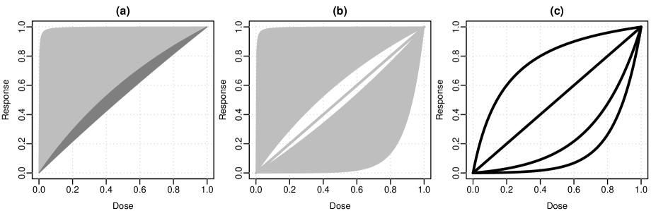
Figure 4: Response curves in the candidate set. The curves were standardized to have effect 0 at dose-level 0 and effect 1 at dose-level 1 (the ``zero-one'' standardization from Figure 2): (a) depicts Emax models for $[0.001,1.5]$ (gray area) and $[0.001,10]$ (gray and dark gray area combined). (b) depicts curves corresponding to the used candidate models: Emax, linear and exponential (c) depicts the candidate curves used for the MCP-Mod methodology

Now suppose we would like to add a linear model $\alpha+\beta z^{(k)}$ to the candidate set of models. The linear model does not use a dose transformation and it represents only a single shape; see also the linear increasing line in Figure 4 (b). Therefore, adding this model does not make the candidate set much broader in terms of shapes, and the critical value only increases to $0.200$. When adding an exponential model of form $\exp(z^{(k)}/\text{})-1$ with parameter bounds $[0.1,2]$, this leads to a more pronounced extension of the possible predictions. This is also reflected in the critical value, which goes up to $0.210$. Figure 4 (b) shows the possible shapes that will be used for the LR test.

So there is a direct, intuitive connection between the critical value and the complexity of the candidate model shapes. The more parts of the unit sphere are covered the larger the multiplicity penalty. On the other hand, when an additional shape is added that is similar to other shapes that are already in the candidate set, the critical value does not increase noticeably, due to the overlap of tubes.

Fitting the dose-response models with the necessary parameter constraints can be done using the fitMod function from the DoseFinding R package. The fitted dose-response functions are shown in Figure 5

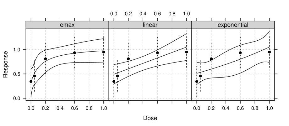
Figure 5: Fitted dose-response functions for biom data-set with 95% pointwise confidence intervals, the means at each dose with 95% confidence intervals are also shown.

The parameter estimates of the models can be found in Table 1, in addition to the p-values for testing $\beta=0$ versus $\beta>0$, for each of the three models. It can be seen that the p-values for the models, considering all three models as candidate set, are all smaller than $0.01$. Of course, this is also true for the p-values that result from considering each model class separately.

Table 1: Results of likelihood-ratio test. The test statistic $R$ is the correlation between the observation and the best model prediction. p-value^∗ is the p-value taking into account the fact that a candidate set of models was used (multiplicity adjustment for the multiple models), while p-value^∗∗ is the p-value within the respective model class (no adjustment for the multiple models).

Model	Parameter estimates	test-statistic	p-value∗	p-value∗∗
Emax ($\text{}\in[0.001,1.5]$)	$\alpha=0.32,\,\beta=0.75,\,\text{}=0.14$	0.335	0.001	0.001
Linear	$\alpha=0.49,\,\beta=0.56$	0.287	0.006	0.002
Exponential ($\text{}\in[0.1,2]$)	$\alpha=0.51,\,\beta=0.83,\,\text{}=2.00$	0.276	0.009	0.004

For comparison we will also apply the MCP-Mod procedure. Similar to Bretz et al. (2005), we choose an Emax shape with $\text{}=0.2$, a linear shape and two exponential shapes, one with $\text{}=0.5/\log(6)$ and the other with $\text{}=0.15$. The candidate shapes of the MCP-Mod procedure are presented in Figure 4 (c). The results shown in Table 2 have been calculated using the MCTtest function in the DoseFinding package. One can see that the Emax and linear model have p-values $<0.01$ similar to the LR test. However, the two exponential shapes have p-values $>0.025$, despite the fact that a trend could be detected using the LR test for the exponential model. The reason is that neither of the two values fits the data well. If the exponential model for $\text{}=2$ would have been included in the set of MCP-Mod candidates also a p-value smaller than $0.01$ would be observed.

After establishing the existence of a dose-response effect, one can continue by either selecting or averaging models to estimate the dose-response curve and the target dose of interest; a detailed discussion of these topics can be found in Schorning et al. (2015).

Table 2: Results of MCP-Mod testing approach.

Shape	test-statistic	p-value
Emax ($\text{}=0.2$)	3.464	0.001
Linear	2.972	0.004
Exponential ($\text{}=0.15$)	2.218	0.028
Exponential ($\text{}=0.5/\log(6)$)	1.898	0.056

3.2 Power calculations for a single Emax model

In this section, we compare the power of the LR test to tests that are optimal for specific values of : assume that the true model is an Emax model with a parameter value ; then, as discussed in Section 2.4, the t-test of $\beta=0$ versus $\beta>0$ in the linear model $y\sim\mathcal{N}(\alpha\mathbf{1}_{n}+\beta x_{\text{}},\sigma^{2}I_{n})$ using the true parameter , is uniformly most powerful invariant. We will refer to this test as locally optimal for . These tests provide a useful upper bound for the performance of the likelihood-ratio test.

Consider again the dose-response trial with dose levels $0,\,0.05,\,0.2,\,0.6,\,1$. We take 20 observations per dose level and choose the non-centrality parameter $\delta=\beta\lVert Bx_{\text{}}\rVert/\sigma$ (Seber and Lee, 2003, Section 6) so that the locally optimal test has power $80\%$ for a one-sided type I error of $5\%$.

For scenarios with different values from $\Gamma=[0.001,1.5]$, we look at the power of a LR test with $\text{}\in\Gamma$, and the power of locally optimal tests for the four parameter values $\text{}=0.001,\,0.035,\,0.159,\,1.5$. These parameter values are chosen so that the corresponding points $x_{\text{}}$ are separated by equal distances along the model curve $\mathbb{M}=\{\tilde{x}_{\text{}}:\text{}\in\Gamma\}$. The critical value of the LR test is given by $0.197$. In Figure 6 it can be seen that the LR test achieves a power above 70% over the whole range of $\Gamma$ and is rather close to the respective locally optimal test. The power of the each locally optimal tests decreases markedly, when the parameter is mis-specified. For example the optimal test for $\text{}=0.001$ has only around 50% power when the true value is $\text{}=0.24$.

Figure 6: Power values of different test procedures in dependence of the true parameter value in the Emax model $x_{\text{}}^{(k)}=z^{(k)}/(z^{(k)}+\text{})$ with 20 observations for each of the dose levels $0,\,0.05,\,0.2,\,0.6,\,1$. Power values of the locally optimal tests for values $0.001,\,0.035,\,0.159,\,1.5$ are shown with dotted and dashed lines. Power values of the likelihood-ratio test with $\Gamma=[0.001,1.5]$ are shown as solid line. The axis for the true values is scaled so that equal distances on the axis correspond to equal distances along the model curve $\text{}\mapsto\tilde{x}_{\text{}}$ of standardized predictions.

3.3 Power calculations for multiple models

We now define five scenarios for the true underlying mean vector: 1) a linear model; 2) an Emax model with parameter $\text{}=0.2$; 3) an exponential model with parameter $\text{}=0.1$; 4) an exponential model with parameter $\text{}=0.5/\log(6)$; and 5) a sigmoid Emax model of the form $x=z^{4}/(z^{4}+0.05^{4})$.

We choose the non-centrality parameter so that in each scenario, the locally optimal test has a power of $50\%$ or $80\%$ for a one-sided type I error of $5\%$. Note that these locally optimal tests are in practice ``unachievable'', as they use information about the true dose-response model class and the true parameter .

The LR test uses the following candidate models: the linear model, the Emax model with $\Gamma=[0.001,1.5]$, and the exponential model with $\Gamma=[0.1,2]$. The critical value of the LR test is given by $0.210$.

For comparison, we consider three multiple contrast tests. First we use Williams contrasts and Marcus contrasts (Williams, 1971; Marcus, 1976), as implemented in the multcomp R package. Both are known to be powerful trend tests. In addition, we use a multiple contrast test with four model-based contrasts (as in MCP-Mod), where the contrasts are optimized to detect the true underlying simulation scenarios 1-4 (see Pinheiro et al. (2014) for details on how to calculate these optimal contrasts). This is unrealistic, as in practice the value of for each model is unknown, but it gives a useful benchmark. Scenario 5) is included to investigate the behaviour for a model shape that is neither part of the LR test nor MCP-Mod set of candidate shapes.

Table 3: Power (in percent) of different test procedures The five scenarios are: 1) a linear model; 2) an Emax model with parameter $\text{}=0.2$; 3) an exponential model with parameter $\text{}=0.1$; 4) an exponential model with parameter $\text{}=0.5/\log(6)$; and 5) a sigmoid Emax model of the form $x=z^{4}/(z^{4}+0.05^{4})$. The non-centrality parameter is chosen so that a local optimal test has either 50% power (first 5 rows) or 80% power (last 5 rows).

			Locally optimal test for scenario
Power	Scenario	LR	1	2	3	4	MCP-Mod	Williams	Marcus
50	1 (Linear)	43.3	50.0	44.1	39.4	45.1	46.8	34.9	43.0
	2 (Emax)	43.4	44.1	50.0	25.3	32.1	44.1	41.1	43.8
	3 (Exp 1)	39.4	39.4	25.3	50.0	48.8	44.1	28.0	37.7
	4 (Exp 2)	41.6	45.1	32.1	48.8	50.0	46.1	30.6	40.2
	5 (Sigm)	41.2	30.7	44.8	15.1	19.5	36.2	44.0	41.2
80	1 (Linear)	73.4	80.0	73.0	66.6	74.3	76.8	61.5	72.9
	2 (Emax)	73.4	73.0	80.0	43.0	55.1	74.5	69.7	73.5
	3 (Exp 1)	69.9	66.6	43.0	80.0	78.6	74.5	52.2	67.8
	4 (Exp 2)	72.1	74.3	55.1	78.6	80.0	76.2	56.0	70.3
	5 (Sigm)	71.1	52.9	73.9	23.2	31.9	65.0	73.6	71.0

In Table 3 one can observe that the performance of the locally optimal tests decreases for the scenarios they are not optimized for, only the locally optimal test corresponding to the linear shape gives a surprisingly good overall performance. Among the multiple contrasts tests the MCP-Mod contrasts, which use information about the true shapes, perform best, apart from the mis-specified scenario 5, where both Williams and Marcus contrasts perform better.

The LR test gives a more robust overall performance. For scenarios 1-4 the power is slightly lower than for the MCP-Mod contrasts, despite the fact that a richer candidate set of models is used. For scenario 5 one can however see that the LR test outperforms the MCP-Mod contrasts. This is most is due to increased robustness (i.e. increased flexibility in model shapes) of the LR test compared to the MCP-Mod contrasts, so that for this shape not included in the candidate set a better performance is obtained.

4 Conclusions

In this manuscript, we have considered the problem of detecting a dose-related trend based on a set of candidate dose-response models.

The problem is not identifiable asymptotically and the standard asymptotic $\chi^{2}$ distribution of the likelihood-ratio statistic does not apply. Furthermore one can show that using a critical value that depends only on the number of parameters in the candidate models and not the model complexity (i.e. the parts covered on the unit sphere) may lead to an arbitrarily large type-I error inflation. To avoid this, we work with the exact small-sample distribution of the likelihood-ratio statistic. Based on a geometric interpretation of the test statistic due to Hotelling, an sampling algorithm has been developed to approximate the exact distribution of the test statistic.

This work extends the previously available methods for dose-response testing in several respects. The multiple contrast tests in MCP-Mod use a fixed set of guesstimates of the nonlinear parameters in the testing step, but then in the modelling step estimates those parameters from the data. We do not require that the parameters in the nonlinear model part are fixed guesstimates, but allow to vary in a defined interval.

An advantage over alternative approaches to derive the distribution of the likelihood ratio test statistic under multiple models (such as those in Dette et al. (2015) and Baayen et al. (2015)) is that we work with the finite sample distribution instead of the asymptotic distribution. In addition to rejection probabilities under the null hypothesis, we also consider rejection probabilities under alternatives. This allows to perform power calculations and thus sample-size calculations at the design stage of an experiment, which is of crucial importance in clinical trials.

The developed methods for calculation of the distribution of the LR test could be of interest beyond dose-response analysis. Nonlinear models, where a test of trend is of interest, appear in many areas of applied sciences such as biology and economics (e.g. change point analysis or harmonic regression).

We have assumed that the residuals are normally distributed. The extension to elliptically contoured distributions is possible directly (Fang and Zhang, 1990; Gupta and Varga, 1993); for other distributions, components of the likelihood-ratio statistic may not be restricted to the unit sphere anymore, but the general approach may still be applied in some situations: for example, Diaconis and Efron (1985) show that the rejection regions of a test for independence in a two-way contingency table are tubular neighborhoods on a simplex on which the test statistic is uniformly distributed under the null hypothesis.

We have also assumed that under the correct model, residuals are independent. The extension to the case of a known correlation structure appears straightforward. More fundamental extensions, such as allowing random effects in addition to the fixed effects, could also be considered.

Another extension would be to test more complicated null hypotheses. For example, a test for a hypothesis $H_{I}$ versus an alternative $H_{J}$ where $I\subseteq J\subseteq\{1,\dots,2m\}$ allows to test individual parameters of a nonlinear model, such as the Hill parameter of the sigmoid Emax model.

The rationale for developing a specialized numerical algorithm for this problem is that direct simulation under the null hypothesis is computationally difficult, since it involves multiple iterative optimizations for each simulation replicate with a poorly identified nonlinear parameter . By using a form of importance sampling it is not necessary to perform nonlinear optimization for the sampling replicates. Note that the developed sampling algorithm might be of interest in general for calculation of the volume of tubes. At the moment dimensionality that the algorithm works on grows with the number of observations, an improvement of the algorithm would be to work with sufficient statistics instead of raw data. This makes the algorithm more efficient, but also more complicated. We also note here that it is numerically advantageous to replace random samples by quasi-random samples (as discussed for example in Fang and Wang (1994)), in which case quasi importance sampling gives a quadrature rule for functions on tubular neighborhoods.

This paper is primarily concerned with testing for a dose-response effect, which is only one of the question of interest in dose-finding studies. Once a dose-response effect has been established the following questions are to estimate the dose-response curve and target doses of interest, so a further topic to explore is the relation between testing and estimation. For (frequentist) model averaging, the predictions are most commonly weighted according to either the AIC or the BIC of the models (see among others Schorning et al. (2015)). Both of these criteria penalize models only according to the number of parameters in the model. We have seen that the number of parameters is, at least for testing, a poor surrogate for the model complexity (the flexibility of the predictions that are possible under a model). Maybe geometric considerations can be used to penalize complex models in a more meaningful way.

Appendix A: Likelihood-ratio statistic for a single parameter value

Theorem 1.

The LR statistic for $H_{0}:\beta=0$ against $H_{i}:\beta\geq 0$ in the linear model $y\sim\mathcal{N}(\alpha\mathbf{1}_{n}+\beta x,\sigma^{2}I_{n})$ has the form $S(R)=(1-\mathbbm{1}{\{R>0\}}R^{2})^{n/2}$, where $R$ is defined in Equation (6) in the paper.

Proof.

Note first that $R=(Bx)^{\top}(By)/(\lVert Bx\rVert\lVert By\rVert)=(Cx)^{\top}(Cy)/(\lVert Cx\rVert\lVert Cy\rVert)$, with $C=I_{n}-n^{-1}\mathbf{1}_{n}\mathbf{1}_{n}^{\top}$ the centering matrix.

Let us first deal with a trivial case:

Case 1:

If $y$ is constant (that is, if $y=\alpha\mathbf{1}_{n}$ for some $\alpha\in\mathbb{R}$), then $R=0$ (since $Cy=\mathbf{0}_{n}$) and $S=1$ (since the likelihood is maximized for $\beta=0$ both under $H_{0}$ and under $H_{i}$).

Assume from now on that $y$ is non-constant. Then the LR statistic has the form [Seber and Lee, 2003, p. 99] $S=(1-T)^{n/2}$ with

$$T=1-\frac{\min_{\alpha\in\mathbb{R},\beta\in\mathbb{R}_{+}}\lVert y-\alpha\mathbf{1}_{n}-\beta x\rVert^{2}}{\min_{\alpha\in\mathbb{R}}\lVert y-\alpha\mathbf{1}_{n}\rVert^{2}}=1-\frac{f(\hat{\beta}_{+})}{f(0)},$$

where $f(\beta)=\lVert C(y-\beta x)\rVert^{2}$ and $\hat{\beta}_{+}=\operatorname{arg\,min}_{\beta\in\mathbb{R}_{+}}f(\beta)$ (with $f(0)>0$ since $y$ is non-constant).

Define $\hat{\beta}_{\pm}=\operatorname{arg\,min}_{\beta\in\mathbb{R}}f(\beta)$. From $\hat{\beta}_{\pm}=(\lVert Cy\rVert/\lVert Cx\rVert)R$, Seber and Lee [2003, p. 139], it follows that

$$\hat{\beta}_{\pm}>0\quad\Longleftrightarrow\quad R>0.$$ (9)

Let us distinguish two cases:

Case 2:

If $R\leq 0$, then $\hat{\beta}_{\pm}\leq 0$ and $\hat{\beta}_{+}=0$ (since $f$ is quadratic in $\beta$), so that

$$T=1-f(0)/f(0)=0.$$ (10)

Case 3:

If $R>0$, then $\hat{\beta}_{\pm}>0$ and $\hat{\beta}_{+}=\hat{\beta}_{\pm}$, so that

$$T=1-f(\hat{\beta}_{\pm})/f(0)$$

From

$$\lVert Cy-(\lVert Cy\rVert/\lVert Cx\rVert)R(Cx)\rVert^{2}=\lVert Cy\rVert^{2}-2\,\underbrace{(\lVert Cy\rVert/\lVert Cx\rVert)R(Cx)^{\top}(Cy)}_{\lVert Cy\rVert^{2}R^{2}}+\underbrace{(\lVert Cy\rVert^{2}/\lVert Cx\rVert^{2})R^{2}\lVert Cx\rVert^{2}}_{\lVert Cy\rVert^{2}R^{2}}$$

we get $f(\hat{\beta}_{\pm})=\lVert Cy\rVert^{2}(1-R^{2})$ and

$$T=1-\frac{\lVert Cy\rVert^{2}(1-R^{2})}{\lVert Cy\rVert^{2}}=R^{2}.$$ (11)

Putting Case 2 and Case 3 together, we obtain $T=\mathbbm{1}{\{R>0\}}R^{2}$, and combining all three cases, we get

$$S(R)=(1-\mathbbm{1}{\{R>0\}}R^{2})^{n/2}.$$ (12)

∎

Appendix B: Counterexample: $\chi^{2}$ critical values

Consider, the model

$$x_{\text{}}=B^{+}\tilde{x}_{\text{}},\qquad\text{}\in\Gamma=[0,2\pi],$$

with $B^{+}$ the Moore-Penrose pseudoinverse of $B$, and

$$\tilde{x}^{(k)}_{\text{}}=\cos\left(\mathbbm{1}{\{k>1\}}\lambda^{k-2}\text{}\right)\prod_{\ell=k}^{d}\sin\left(\lambda^{\ell-1}\text{}\right),\quad k=1,\dots,{d+1},$$

for some constant $\lambda\in\mathbb{N}$. The standardized predictions, $\tilde{x}_{\text{}}$, are the Cartesian coordinates of a point with spherical coordinates $\text{},\,\lambda\text{},\,\dots,\lambda^{d-1}\text{}$. Since $\sup_{\psi\in[0,2\pi]^{d}}\inf_{\text{}\in\Gamma}\lVert\psi-(\text{}\bmod 2\pi,\,\lambda\text{}\bmod 2\pi,\,\dots,\lambda^{d-1}\text{}\bmod 2\pi)^{\top}\rVert\to 0$, also $\inf_{\tilde{y}\in\mathbb{S}}\sup_{\text{}\in\Gamma}\tilde{y}^{\top}\tilde{x}_{\text{}}\to 1$, as $\lambda\to\infty$. Therefore, for any $q$, we can choose a constant $\lambda$ so that $R>(1-\exp(-q/n))^{1/2}$ for all $\tilde{y}\in\mathbb{S}$, which ensures that $-2\log S>q$.

The plot in the right-hand side of Figure 2 in the paper illustrates the construction when $d=2$. As goes from 0 to $\pi$, the spiral curve $\text{}\mapsto\tilde{x}_{\text{}}$ takes $\lambda$ rotations around the sphere. For any $r<1$, one can choose $\lambda$ large enough to make the tubular neighborhood around $\mathbb{M}$ cover the complete sphere. Note that both of the models in Figure 2 have the same number of parameters but their complexities (in terms of the possible predictions) are vastly different.

Appendix C: Details on the numerical calculation of tubular volumes

Assume that we have some way to sample a point $W$ with support $\mathbb{M}$. Let us say that this point has distribution $H$ on $\mathbb{M}$, even if we do not know $H$ explicitly. For the sake of illustration, here is one simple way to sample such a point: start by selecting a model $i$ from the $m$ models with equal probability, then sample a value from $\Gamma_{i}$ according to some convenient distribution and finally take $W=\tilde{x}_{\text{},i}$.

Next, we sample a point $V$ from $G_{W}$, the uniform probability distribution on the spherical cap $\mathbb{C}_{Wr}$. The joint distribution is $P(V\in T,W\in M)=\int_{M}G_{w}(T)\mathrm{d}H(w)$, for Borel sets $T\subseteq\mathbb{T}_{r}$ and $M\subseteq\mathbb{M}$. By Fubini's theorem, $\int_{M}G_{w}(T)\,\mathrm{d}H(w)=\int_{T}\int_{M}g_{w}(v)\,\mathrm{d}H(w)\,\mathrm{d}\varsigma(v)$, with $g_{w}(v)=\mathbbm{1}{\{w\in\mathbb{C}_{vr}\}}/\varsigma(\mathbb{C}_{vr})$ the density of $G_{w}$ with respect to $\varsigma$. Let us define $c_{r}=\varsigma(\mathbb{C}_{vr})=\left\lvert\mathbb{C}_{r}\right\rvert/\left\lvert\mathbb{S}\right\rvert$. The value of $c_{r}$ is given in Equation (7) in the main text. Then, the random point $V$ has density

$$g(v)=\frac{1}{c_{r}}\int_{\mathbb{M}}\mathbbm{1}{\{w\in\mathbb{C}_{vr}\}}\,\mathrm{d}H(w)=\frac{1}{c_{r}}P(W\in\mathbb{C}_{vr}).$$

If we repeat this procedure $\kappa$ times, we obtain a sample $(V_{1},W_{1}),\dots,(V_{\kappa},W_{\kappa})$. Approximating $P(W\in\mathbb{C}_{vr})$ by relative frequencies gives $g(v)\approx\left\lvert\{j:W_{j}\in\mathbb{C}_{vr}\}\right\rvert/(\kappa c_{r})$. In this way, we arrive at the approximation

$$\int_{\mathbb{T}_{r}}f\,\mathrm{d}\varsigma\approx c_{r}\sum_{k=1}^{\kappa}\frac{f(V_{k})}{\left\lvert\{j:W_{j}\in\mathbb{C}_{V_{k}r}\}\right\rvert}.$$ (13)

Note that we work with points on the $d$-dimensional unit sphere, which becomes difficult when the sample size becomes large. It is, however, possible to modify the algorithm, and work with sufficient statistics instead of raw data. To keep the presentation brief, the details are not given here. Algorithm 1 outlines the main steps of the procedure.

for $k\leftarrow 1$ to $\kappa$ do

       sample $W_{k}$ from the distribution $H$ on $\mathbb{M}$;

       sample $V_{k}$ from $G_{W_{k}}$ on $\mathbb{C}_{W_{k},r}$;

      

end for

for $k\leftarrow 1$ to $\kappa$ do

       Calculate $m_{k}=\left\lvert\{j:W_{j}\in\mathbb{C}_{V_{k}r}\}\right\rvert$;

      

end for

Result: $c_{r}\sum_{k=1}^{\kappa}f(V_{k})/m_{k}$

Algorithm 1 Sampling algorithm

Theorem 2 below shows that the right-hand side of Equation (13) converges in probability to the left-hand side as $\kappa\to\infty$. Hence, the approximation error can be made arbitrarily small by increasing the number of sampling replicates $\kappa$.

Definition 1.

In the following, we will call a family $Y_{nj}$, with $j=1,\dots,n$ and $n=1,2,\dots$, of random vectors a triangular arrangement, if for each $n$, the random vectors $Y_{n1},\dots,Y_{nn}$ are iid and have finite expectations and variances.

Theorem 2.

Let $\mathbb{M}$ be a Borel set on $\mathbb{S}$ and let $\mathbb{T}_{r}$ denote the tubular neighborhood around $\mathbb{M}$ with radius $r$. Consider a sequence $w_{n}$ in $\mathbb{M}$ so that $\left\lvert\{j:1\leq j\leq n\ \text{and}\ w_{j}\in\mathbb{C}_{vr}\}\right\rvert\to\infty$ as $n\to\infty$ for each $v$ in the interior of $\mathbb{T}_{r}$. Also consider a sequence of independent random vectors $V_{n}\sim\mathcal{U}(\mathbb{C}_{w_{n},r})$, uniformly distributed on the spherical cap $\mathbb{C}_{w_{n},r}$. Let $f:\mathbb{S}\to\mathbb{R}_{+}$ be Borel and bounded. Define the sequence of functions $g_{n}:\mathbb{T}_{rn}\to\mathbb{R}_{+}$, on $\mathbb{T}_{rn}=\cup_{j=1}^{n}\mathbb{C}_{w_{j},r}$, by $g_{n}(v)=(n\,\psi_{n}(v)\varsigma(\mathbb{C}_{vr}))^{-1}$ with $\psi_{n}(v)=1/\left\lvert\{j:1\leq j\leq n\ \text{and}\ w_{j}\in\mathbb{C}_{vr}\}\right\rvert$ and $\varsigma$ the uniform probability measure on $\mathbb{S}$. Also define the random variables $X_{n}=f(V_{n})/g_{n}(V_{n})$ and $S_{n}=(X_{1}+\dots+X_{n})/n$. Then $S_{n}\stackrel{{\scriptstyle P}}{{\to}}\int_{\mathbb{T}_{r}}f\,\mathrm{d}\varsigma$.

Proof.

Consider the triangular arrangements $K_{nj}$ and $V_{nj}^{\prime}$ and $X_{nj}^{\prime}$, where $K_{nj}\sim\mathcal{U}(\{1,\dots,n\})$, where $V_{nj}^{\prime}\,|\,(K_{nj}=k)\sim\mathcal{U}(\mathbb{C}_{w_{k},r})$, and where $X_{nj}^{\prime}=f(V_{nj}^{\prime})/g_{n}(V_{nj}^{\prime})$. Define $S_{n}^{\prime}=(X_{n1}^{\prime}+\dots+X_{nn}^{\prime})/n$. Due to Lemma 1 below, it suffices to show that $E(S_{n}^{\prime})\to\int_{\mathbb{T}_{r}}f\,\mathrm{d}\varsigma$ and $\operatorname{Var}(S_{n}^{\prime})\to 0$.

First, the argument for $E(S_{n}^{\prime})\to\int_{\mathbb{T}_{r}}f\,\mathrm{d}\varsigma$. For each $n$, the variables $X_{n1}^{\prime},\dots X_{nn}^{\prime}$ are iid; hence $E(S_{n}^{\prime})=E(X_{n1}^{\prime})$. Since $V_{n1}^{\prime}$ has density $g_{n}$ on $\mathbb{T}_{rn}$ (with respect to $\varsigma$),

$$E(X_{n1}^{\prime})=E\left(\frac{f(V_{n1}^{\prime})}{g_{n}(V_{n1}^{\prime})}\right)=\int_{\mathbb{T}_{rn}}\frac{f(v)}{g_{n}(v)}g_{n}(v)\mathrm{d}\varsigma(v)=\int_{\mathbb{T}_{rn}}f\,\mathrm{d}\varsigma.$$

Now $\mathbb{T}_{r,1}\subseteq\mathbb{T}_{r,2}\subseteq\dots$ is an increasing sequence of subsets of $\mathbb{T}_{r}$, and $\left\lvert\mathbb{T}_{r}\setminus\mathbb{T}_{rn}\right\rvert\to 0$ by the assumptions on the sequence $w_{n}$; therefore, by the monotone convergence theorem, $E(S_{n}^{\prime})=\int_{\mathbb{T}_{r}}\mathbbm{1}{\{v\in\mathbb{T}_{rn}\}}f(v)\,\mathrm{d}\varsigma(v)\to\int_{\mathbb{T}_{r}}f\,\mathrm{d}\varsigma$.

Second, the argument for $\operatorname{Var}(S_{n}^{\prime})\to 0$. Integrating with respect to the density $g_{n}$ of $V_{n1}^{\prime}$ gives

$$\operatorname{Var}(X_{n1}^{\prime})=E\bigl{(}(X_{n1}^{\prime})^{2}\bigr{)}-\bigl{(}E(X_{n1}^{\prime})\bigr{)}^{2}\leq\int_{\mathbb{T}_{rn}}\frac{f(v)^{2}}{g_{n}(v)}\,\mathrm{d}\varsigma(v).$$

Let $M=\sup_{v\in\mathbb{T}_{rn}}f(v)^{2}\varsigma(\mathbb{C}_{vr})$, which is finite since $f$ is bounded. Then $\operatorname{Var}(X_{n1}^{\prime})\leq nM\int_{\mathbb{T}_{rn}}\psi_{n}\,\mathrm{d}\varsigma$. Furthermore, $\operatorname{Var}(S_{n}^{\prime})=\operatorname{Var}(X_{n1}^{\prime})/n$ since $X_{n1}^{\prime},\dots X_{nn}^{\prime}$ are iid; thus $\operatorname{Var}(S_{n}^{\prime})\leq M\int_{\mathbb{T}_{rn}}\psi_{n}\,\mathrm{d}\varsigma$. But $\psi_{n}(v)\to 0$ for every $v$ in the interior of $\mathbb{T}_{r}$ and the boundary of $\mathbb{T}_{r}$ has measure zero, so that $\operatorname{Var}(S_{n}^{\prime})\to 0$ by the dominated convergence theorem. ∎

Lemma 1.

Consider a sequence of independent random variables $X_{n}$ and two triangular arrangements $K_{nj}$ and $X_{nj}^{\prime}$, where $K_{nj}\sim\mathcal{U}(\{1,\dots,n\})$ and $X_{nj}^{\prime}\,|\,(K_{nj}=k)\stackrel{{\scriptstyle d}}{{=}}X_{k}$. Define $S_{n}=(X_{1}+\dots+X_{n})/n$ and $S_{n}^{\prime}=(X_{n_{1}}^{\prime}+\dots+X_{nn}^{\prime})/n$. If $E(S_{n}^{\prime})\to\alpha$ for some value $\alpha\in\mathbb{R}$ and $\operatorname{Var}(S_{n}^{\prime})\to 0$, then $S_{n}\stackrel{{\scriptstyle P}}{{\to}}\alpha$.

Proof.

Fix a value $\epsilon>0$. For every $n\in\mathbb{N}$,

$$E(S_{n})=\frac{1}{n}\sum_{j=1}^{n}E(X_{j})=E(E(X_{n1}^{\prime}\,|\,K_{n1}))=E(X_{n1}^{\prime})=E(S_{n}^{\prime}).$$

Hence there exists an $m\in\mathbb{N}$ so that $\left\lvert E(S_{n})-\alpha\right\rvert<\epsilon/2$, for all $n>m$.

It follows that for such $n>m$ also $P(\left\lvert S_{n}-\alpha\right\rvert>\epsilon)\leq P(\left\lvert S_{n}-E(S_{n})\right\rvert>\epsilon/2)$. By Chebyshev's inequality $P(\left\lvert S_{n}-E(S_{n})\right\rvert>\epsilon/2)\leq 4\operatorname{Var}(S_{n})/\epsilon^{2}$. Consequently, if $\operatorname{Var}(S_{n})\to 0$, then $P(\left\lvert S_{n}-\alpha\right\rvert>\epsilon)\to 0$. And $\operatorname{Var}(S_{n})\to 0$ follows from

$$\begin{split}\operatorname{Var}(S_{n})&=\frac{1}{n^{2}}\sum_{k=1}^{n}\operatorname{Var}(X_{k})\\ &=\frac{1}{n}E(\operatorname{Var}(X_{n1}^{\prime}\,|\,K_{n1}))\\ &\leq\frac{1}{n}\Bigl{(}E(\operatorname{Var}(X_{n1}^{\prime}\,|\,K_{n1}))+\operatorname{Var}(E(X_{nj}^{\prime}\,|\,K_{n1}))\Bigr{)}\\ &=\frac{1}{n}\operatorname{Var}(X_{n1}^{\prime})=\operatorname{Var}(S_{n}^{\prime}),\end{split}$$

where the last line uses the well known equation for the conditional variance (see, e.g., Proposition 5.2 in Ross [2011]). ∎

References

- Andrews [1996] D. Andrews. Admissibility of the likelihood ratio test when the parameter space is restricted under the alternative. Econometrica, 64:705–718, 1996.
- Andrews and Ploberger [1994] D. Andrews and W. Ploberger. Optimal tests when a nuisance parameter is present only under the alternative. Econometrica, 62:1383–1414, 1994.
- Andrews and Ploberger [1995] D. Andrews and W. Ploberger. Admissibility of the likelihood ratio test when a nuisance parameter is present only under the alternative. The Annals of Statistics, 23:1609–1629, 1995.
- Baayen et al. [2015] C. Baayen, P. Hougaard, and C. B. Pipper. Testing effect of a drug using multiple nested models for the dose-response. Biometrics, 71:417–427, 2015.
- Bornkamp et al. [2009] B. Bornkamp, J. C. Pinheiro, and F. Bretz. MCPMod: An R package for the design and analysis of dose-finding studies. Journal of Statistical Software, 29(7):1–23, 2009.
- Bretz et al. [2005] F. Bretz, J. C. Pinheiro, and M. Branson. Combining multiple comparisons and modeling techniques in dose-response studies. Biometrics, 61:738–748, 2005.
- Chatfield [1995] C. Chatfield. Model uncertainty, data mining and statistical inference. Journal of the Royal Statistical Society, Series A, 158:419–466, 1995.
- Claeskens and Hjort [2008] G. Claeskens and N. L. Hjort. Model Selection and Model Averaging. Cambridge University Press, Cambridge, 2008.
- Davies [1977] R. B. Davies. Hypothesis testing when a nuisance parameter is present only under the alternative. Biometrika, 64:247–254, 1977.
- Davies [1987] R. B. Davies. Hypothesis testing when a nuisance parameter is present only under the alternative. Biometrika, 74:33–43, 1987.
- Dette et al. [2015] H. Dette, S. Titoff, S. Volgushev, and F. Bretz. Dose response signal detection under model uncertainty. Biometrics, 2015. Epub ahead of print.
- Diaconis and Efron [1985] P. Diaconis and B. Efron. Testing for independence in a two-way table: new interpretations of the chi-square statistic. The Annals of Statistics, 13:845–874, 1985.
- Dragalin et al. [2007] V. Dragalin, F. Hsuan, and S. K. Padmanabhan. Adaptive designs for dose-finding studies based on the sigmoid emax model. Journal of Biopharmaceutical Statistics, 17:1051–1070, 2007.
- European Medicines Agency [2014] European Medicines Agency. Qualification opinion of MCP-Mod as an efficient statistical methodology for model-based design and analysis of Phase II dose finding studies under model uncertainty, 2014. http://goo.gl/imT7IT.
- Fang and Zhang [1990] K. Fang and Y. Zhang. Generalized multivariate analysis. Science Press, 1990.
- Fang and Wang [1994] K.-T. Fang and Y. Wang. Number-theoretic Methods in Statistics. Chapmann and Hall, London, 1994.
- Gray [2004] A. Gray. Tubes. Birkhäuser, 2nd edition, 2004.
- Grieve and Krams [2005] A. P. Grieve and M. Krams. ASTIN: a Bayesian adaptive dose-response trial in acute stroke. Clinical Trials, 2:340–351, 2005.
- Gupta and Varga [1993] A. Gupta and T. Varga. Elliptically Contoured Models in Statistics. Springer, 1993.
- Hotelling [1939] H. Hotelling. Tubes and spheres in n-spaces, and a class of statistical problems. American Journal of Mathematics, 61:440–460, 1939.
- Johansen and Johnstone [1990] S. Johansen and I. M. Johnstone. Hotelling's theorem on the volume of tubes: Some illustrations in simulatenous inference and data analysis. Annals of Statistics, 18:652–684, 1990.
- Jones et al. [2011] B. Jones, G. Layton, H. Richardson, and N. Thomas. Model-based Bayesian adaptive dose-finding designs for a phase II trial. Statistics in Biopharmaceutical Research, 3:276–287, 2011.
- Leeb and Pötscher [2005] H. Leeb and B. M. Pötscher. Model selection and inference: Facts and fiction. Econometric Theory, 21:21–59, 2005.
- Lehmann and Romano [2008] E. Lehmann and J. Romano. Testing Statistical Hypotheses. Springer, New York, 3rd edition, 2008.
- Li [2011] S. Li. Concise formulas for the area and volume of a hyperspherical cap. Asian Journal of Mathematics and Statistics, 4:66–70, 2011.
- Liu and Shao [2003] X. Liu and Y. Shao. Asymptotics for likelihood ratio tests under loss of identifiability. Annals of Statistics, 31:807–832, 2003.
- Marcus [1976] R. Marcus. The power of some tests for the equality of normal means against an ordered alternative. Biometrika, 63:177–183, 1976.
- Naiman [1990] D. Naiman. On volumes of tubular neighborhoods of spherical polyhedra and statistical inference. The Annals of Statistics, 18:685–716, 1990.
- Pinheiro et al. [2014] J. C. Pinheiro, B. Bornkamp, E. Glimm, and F. Bretz. Model-based dose finding under model uncertainty using general parametric models. Statistics in Medicine, 33:1646–1661, 2014.
- Pukkila and Rao [1988] T. Pukkila and R. Rao. Pattern recognition based on scale invariant discriminant functions. Information sciences, 45:379–389, 1988.
- Ritz and Skovgaard [2005] C. Ritz and I. M. Skovgaard. Likelihood ratio tests in curved exponential families with nuisance parameters present only under the alternative. Biometrika, 92:507–517, 2005.
- Ross [2011] S. Ross. A First Course in Probability. Prentice Hall, 8th edition, 2011.
- Schorning et al. [2015] K. Schorning, B. Bornkamp, F. Bretz, and H. Dette. Model selection versus model averaging in dose finding studies. Technical Report, 2015. http://arxiv.org/pdf/1508.00281.pdf.
- Seber and Lee [2003] G. Seber and A. Lee. Linear Regression Analysis. Wiley, 2nd edition, 2003.
- Thomas [2006] N. Thomas. Hypothesis testing and Bayesian estimation using a sigmoid Emax model applied to sparse dose designs. Journal of Biopharmaceutical Statistics, 16:657–677, 2006.
- Weyl [1939] H. Weyl. On the volume of tubes. American Journal of Mathematics, 61:461–472, 1939.
- Williams [1971] D. A. Williams. A test for difference between treatment means when several dose levels are compared to a zero dose control. Biometrics, 27:103–117, 1971.