Watson’s theorem and the $N\Delta(1232)$ axial transition

Abstract

We present a new determination of the $N\Delta$ axial form factors from neutrino induced pion production data. For this purpose, the model of Hernandez et al., Phys. Rev. D 76, 033005 (2007) is improved by partially restoring unitarity. This is accomplished by imposing Watson’s theorem on the dominant vector and axial multipoles. As a consequence, a larger $C_{5}^{A}(0)$, in good agreement with the prediction from the off-diagonal Goldberger-Treiman relation, is now obtained.

I Introduction

Weak pion production off nucleons provides valuable insight into the axial structure of hadrons. In addition, pion production cross sections grow to become one of the main reaction mechanisms for neutrinos of few-GeV energies, which is an important range for current and future oscillation experiments. Therefore, a better understanding of weak pion production mechanisms is actively pursued Morfin et al. (2012); Formaggio and Zeller (2012); Alvarez-Ruso et al. (2014). Recent measurements on, predominantly, carbon targets by MiniBooNE Aguilar-Arevalo et al. (2010, 2011a, 2011b) and MINERvA Aguilar-Arevalo et al. (2011b); Le et al. (2015) experiments have revealed discrepancies with existing theoretical models and among different data sets Lalakulich and Mosel (2013); Hernández et al. (2013); Yu et al. (2015); Sobczyk and Zmuda (2015); Mosel (2015).

The first requirement to achieve a precise knowledge of neutrino induced pion production on nuclear targets is a realistic model at the nucleon level. Theoretical studies of weak pion production off the nucleon at intermediate energies Adler (1968); Bijtebier (1970); Zucker (1971); Llewellyn Smith (1972); Schreiner and Von Hippel (1973); Alevizos et al. (1977); Fogli and Nardulli (1979, 1980); Rein and Sehgal (1981); Hemmert et al. (1995); Alvarez-Ruso et al. (1998, 1999); Slaughter (2002); Golli et al. (2003); Sato et al. (2003); Paschos et al. (2004); Lalakulich and Paschos (2005); Lalakulich et al. (2006); Hernandez et al. (2007); Graczyk and Sobczyk (2008); Leitner et al. (2009); Barbero et al. (2008); Graczyk et al. (2009); Hernandez et al. (2010); Lalakulich et al. (2010); Serot and Zhang (2012); Barbero et al. (2014); Zmuda and Graczyk (2015); Nakamura et al. (2015); Alam et al. (2015) have highlighted the important role of baryon resonance excitation, predominantly the $\Delta(1232)3/2^{+}$. The weak nucleon-to-$\Delta(1232)$ transition current can be written in terms of vector and axial form factors, $C_{3-5}^{V}$ and $C_{3-6}^{A}$ in the notation of Ref. Llewellyn Smith (1972). Although there are quark model determinations of these form factors Feynman et al. (1971); Liu et al. (1995); Golli et al. (2003); Barquilla-Cano et al. (2007), a common strategy is to adopt empirical parametrizations for them. The role of heavier resonances has also been investigated although the available experimental information about the axial sector is very limited. Among these states, only the $N(1520)3/2^{-}$ appears to be relevant for neutrino energies below 1.5 GeV Leitner et al. (2009). Nonresonant electroweak amplitudes have also been extensively considered. As pointed out in Ref. Hernandez et al. (2007), these terms are not only demanded but, close to threshold, fully fixed by chiral symmetry. Away from threshold, these amplitudes are usually modeled using phenomenologically parametrized nucleon form factors, introduced in a way that respects both the conservation of the vector current (CVC) and the partial conservation of the axial current (PCAC).

In Ref. Hernandez et al. (2007) (referred from now on as the HNV model) nonresonant amplitudes, evaluated from the leading contributions of the SU(2) chiral Lagrangian, supplemented with empirical parametrizations of the nucleon form factors, were considered alongside the $\Delta(1232)$ excitation. The vector form factors in the $N\Delta$ vertex come from helicity amplitudes extracted in the analysis of electron scattering data Lalakulich and Paschos (2005). The most important among the axial form factors is $C^{A}_{5}$, which appears at leading order in an expansion of the hadronic tensor in the four-momentum transfer $q^{2}$. Assuming the pion pole dominance of the pseudoscalar form factor $C^{A}_{6}$, it can be related to $C^{A}_{5}$ owing to PCAC. For the subleading $C_{3,4}^{A}$ form factors, Adler’s parametrizations Adler (1968); Bijtebier (1970) were adopted: $C_{3}^{A}=0,C_{4}^{A}=-C_{5}^{A}/4$. The available bubble-chamber data on pion production induced by neutrinos on deuterium, taken at Argonne and Brookhaven National Laboratories (ANL and BNL) Radecky et al. (1982); Kitagaki et al. (1986) are quite insensitive to the values of these form factors Hernandez et al. (2010). With the aim of extending the model toward higher energies, the $N(1520)$ intermediate state was added in Ref. Hernández et al. (2013) using the transition form factors introduced in Ref. Leitner et al. (2009).

The pion pole dominance of $C^{A}_{6}$ and PCAC result in a relation between the leading axial coupling $C_{5}^{A}(q^{2}=0)$ and the $\Delta\rightarrow N\pi$ decay coupling known as the off-diagonal Goldberger-Treiman relation (GTR). Studies that neglected the nonresonant contributions found good agreement between the $C_{5}^{A}(0)$ value extracted from ANL and/or BNL data and the GTR Alvarez-Ruso et al. (1999); Graczyk et al. (2009). However, the fit of $C_{5}^{A}(q^{2})$ to the flux averaged $\nu_{\mu}p\to\mu^{-}p\pi^{+}$ ANL $q^{2}$-differential cross section data Radecky et al. (1982) with the HNV model found a discrepancy of 30% with respect to the GTR prediction of $C_{5}^{A}(0)=1.15-1.2$. A simultaneous fit to both ANL and BNL data samples including independent overall flux normalization uncertainties for each experiment, as suggested in Ref. Graczyk et al. (2009), and considering deuterium-target corrections obtained $C_{5}^{A}(0)=1.00\pm 0.11$ Hernandez et al. (2010), still 2$\sigma$ below the GTR value. Although the HVN model could be reconciled with the GTR by simultaneously fitting vector form factors to electron-proton scattering structure function $F_{2}$ Graczyk et al. (2014); Zmuda and Graczyk (2015), it should be realized that the HNV model does not satisfy Watson’s theorem Watson (1952). The latter, which is a consequence of unitarity and time-reversal invariance, implies that the phase of the electroweak pion production is fully determined by the strong $\pi N$ interaction. The goal of the present study is to impose Watson’s theorem in the HNV model. It is shown that, in this way, the consistency with the GTR prediction is restored.

The dynamical model of photo-, electro- and weak pion production derived in Ref. Sato et al. (2003) deserves a special mention. To date, this is the only weak pion production model fulfilling Watson’s theorem exactly. Starting from an effective Hamiltonian with bare $N\Delta$ couplings obtained in a nonrelativistic constituent quark model Hemmert et al. (1995), the Lippmann-Schwinger equation in coupled channels is solved, which restores unitarity. Besides, the bare couplings get renormalized by meson clouds. The predicted cross sections are in good agreement with data (Figs. 5-8 of Ref. Sato et al. (2003)). The scheme has been further refined and extended to incorporate $N^{*}$ resonances and a larger number of meson-baryon states Kamano et al. (2012); Nakamura et al. (2015). Although the chiral counting at threshold is broken by the presence of $\rho$ and $\omega$ exchanges in the $t$-channel or the introduction of explicit $\sigma$ meson intermediate states, this framework should satisfy unitary constraints and fulfill Watson’s theorem. The partially unitarized HNV model presented here is considerably simpler. The agreement with the GTR and a good description of data for invariant masses $W_{\pi N}<1.4$ GeV are achieved by introducing two relative phases between the $\Delta(1232)$ and the nonresonant contributions. The HNV model improved in this way is portable and can be easily implemented in event generators used in the analysis of neutrino oscillation experiments.

The paper is organized as follows. In Sec. II, we introduce Watson’s theorem, which is based on unitarity and time reversal invariance, and explain its implementation in the HNV model. In Sec. III we present the new extraction of the $C_{5}^{A}(q^{2})$ axial form factor. Appendices A,B and C collect some useful formulas needed for the calculation. Finally, in Appendix D we give a parametrization of the Olsson phases (see below) used to impose Watson’s theorem in our approach.

II Unitarity, time-reversal invariance and Watson’s theorem

A scattering process due to short-range interactions (like strong or weak interactions) can be described in terms of initial and final states of noninteracting particles. The amplitude for a transition is given by the corresponding matrix element of the scattering operator

$$S=\mbox{1}\rule{0.28453pt}{6.45831pt}\hskip 4.30554pt-iT\,.$$ (1)

Given an initial state $|I\rangle$, the probability for finding the system in an asymptotic state $|N\rangle$ is $P_{N}=|\langle N|S|I\rangle|^{2}$; since $\sum_{N}P_{N}=1$, one deduces that $S$ is a unitary operator, $SS^{\dagger}=S^{\dagger}S=\mbox{1}\rule{0.28453pt}{6.45831pt}\hskip 4.30554pt$, which implies that

$$i(T-T^{\dagger}) = T^{\dagger}T\,$$

$$i\big{\{}\langle F|T|I\rangle-\langle F|T^{\dagger}|I\rangle\big{\}} = \langle F|T^{\dagger}T|I\rangle=\sum_{N}\langle F|T^{\dagger}|N\rangle\langle N|T|I\rangle=\sum_{N}\langle N|T|F\rangle^{*}\langle N|T|I\rangle\,.$$ (3)

On the other hand, if time reversal invariance holds,

$$\langle F|S|I\rangle=\langle I_{\mathscr{T}}|S|F_{\mathscr{T}}\rangle\,,$$ (4)

where $\mathscr{T}|I\rangle=|I_{\mathscr{T}}\rangle$ and $\mathscr{T}|F\rangle=|F_{\mathscr{T}}\rangle$. In other words, if the system is time reversal invariant, $\mathscr{T}S\mathscr{T}^{\dagger}=S^{\dagger}$ and therefore $\mathscr{T}^{\dagger}T^{\dagger}\mathscr{T}=T$. The time reversal operator $\mathscr{T}$ is antiunitary Martin and Spearman (1970); Gibson and Pollard (1980) with $\mathscr{T}^{2}=\pm\mbox{1}\rule{0.28453pt}{6.45831pt}\hskip 4.30554pt$. Thus, one finds

$$\langle F|T^{\dagger}|I\rangle=\langle I|T|F\rangle^{*}=\langle I|\mathscr{T}^{\dagger}T^{\dagger}\mathscr{T}|F\rangle^{*}=\langle I_{\mathscr{T}}|T^{\dagger}|F_{\mathscr{T}}\rangle=\langle F_{\mathscr{T}}|T|I_{\mathscr{T}}\rangle^{*}\,.$$ (5)

Using this result in Eq. (3), we obtain from unitarity and time reversal invariance that

$$i\big{\{}\langle F|T|I\rangle-\langle F_{\mathscr{T}}|T|I_{\mathscr{T}}\rangle^{*}\big{\}}=\sum_{N}\langle N|T|F\rangle^{*}\langle N|T|I\rangle$$ (6)

If $\langle F|T|I\rangle=\langle F_{\mathscr{T}}|T|I_{\mathscr{T}}\rangle$, which is always satisfied for transitions between center of mass (CM) two-particle states with well defined helicities and total angular momentum whenever the interaction is invariant under time reversal Martin and Spearman (1970), and there is only one relevant intermediate state in the sum of Eq. (6), one obtains that

$$\langle N|T|F\rangle^{*}\langle N|T|I\rangle=-2\,{\rm Im}\langle F|T|I\rangle\in\mbox{R}\rule{0.28453pt}{6.45831pt}\hskip 4.30554pt\,$$ (7)

so that the phases of $\langle N|T|F\rangle$ and $\langle N|T|I\rangle$ coincide. This result constitutes Watson’s theorem Watson (1952) on the effect of final state interactions on reaction cross sections. As shown, it is a consequence of unitarity and time reversal invariance.

II.1 Watson’s theorem for CM two-particle helicity states

Assuming that only two-particle intermediate states (2body), with masses $m_{1}^{\prime}$ and $m_{2}^{\prime}$, contribute, the unitarity condition of Eq. (3) for the binary process $a+b\to 1+2$ can be written as

$$i\left\{\langle\theta,\varphi;\lambda_{1},\lambda_{2};\gamma_{12}\,|T(s)|0,0;\lambda_{a},\lambda_{b};\gamma_{ab}\,\rangle-\langle\theta,\varphi;\lambda_{1},\lambda_{2};\gamma_{12}\,|T^{\dagger}(s)|0,0;\lambda_{a},\lambda_{b};\gamma_{ab}\,\rangle\right\}=\sum_{\rm 2body}\frac{\lambda^{1/2}(s,m_{1}^{\prime\,2},m_{2}^{\prime\,2})}{32\pi^{2}s}$$ (8)

$$\times \int d\Omega^{\prime}\sum_{\gamma^{\,\prime}_{12}}\sum_{\lambda^{\prime}_{1}\lambda^{\prime}_{2}}\langle\theta^{\prime},\varphi^{\prime};\lambda^{\prime}_{1},\lambda^{\prime}_{2};\gamma^{\,\prime}_{12}\,|T(s)|\theta,\varphi;\lambda_{1},\lambda_{2};\gamma_{12}\,\rangle^{*}\langle\theta^{\prime},\varphi^{\prime};\lambda^{\prime}_{1},\lambda^{\prime}_{2};\gamma^{\,\prime}_{12}\,|T(s)|0,0;\lambda_{a},\lambda_{b};\gamma_{ab}\,\rangle\,$$

where $s=(p_{a}+p_{b})^{2}$ and the function $\lambda(x,y,z)=x^{2}+y^{2}+z^{2}-2xy-2xz-2yz$. Two-particle states in the CM are defined in Appendix A. The matrix element of the $T$ operator is computed in the little Hilbert space (see Appendix A and the book of Martin & Spearman Martin and Spearman (1970))

$$\langle\theta,\varphi;\lambda_{1},\lambda_{2};\gamma_{12}\,|T(s)|0,0;\lambda_{a},\lambda_{b};\gamma_{ab}\,\rangle\equiv\langle\alpha_{F}|T_{P}|\alpha_{I}\rangle=\frac{(2\pi)^{2}4\sqrt{s}}{\sqrt{|\vec{p}_{I}||\vec{p}_{F}|}}\langle\theta,\varphi;\lambda_{1},\lambda_{2};\gamma_{12}\,|T_{P}|0,0;\lambda_{a},\lambda_{b};\gamma_{ab}\,\rangle\equiv T_{FI}(s)$$ (9)

where $|\vec{p}_{I(F)}|\equiv|\vec{p}_{a(1)}|=|\vec{p}_{b(2)}|$; $T_{P}$ is the reduction of the full operator $T$ in the little Hilbert space, Eq. (47). Normalizations are fixed by the expression of the CM differential cross section for the $a+b\to 1+2$ reaction, which is calculated as

$$\frac{d\sigma}{d\Omega}=\frac{1}{64\pi^{2}s}\frac{|\vec{p}_{F}|}{|\vec{p}_{I}|}\left|T_{FI}(s)\right|^{2}$$ (10)

The unitarity condition, Eq. (8), can be rewritten for states $|J,M\rangle$ with well-defined angular momentum. Changing basis with Eq. (51) and using the orthogonality properties of the ${\cal D}^{(J)}_{MM^{\prime}}(\varphi,\theta,-\varphi)$ rotation matrices [Eq. (53)], the condition ${\cal D}^{(J)}_{MM^{\prime}}(0,0,0)=\delta_{MM^{\prime}}$, the fact that $T$ is a scalar under rotations, and Parseval’s identity associated to Eq. (49), one gets that

$$i \left\{\langle J,M;\lambda_{1},\lambda_{2};\gamma_{12}\,|T(s)|J,M;\lambda_{a},\lambda_{b};\gamma_{ab}\,\rangle-\langle J,M;\lambda_{1},\lambda_{2};\gamma_{12}\,|T^{\dagger}(s)|J,M;\lambda_{a},\lambda_{b};\gamma_{ab}\,\rangle\right\}=\sum_{\rm 2body}\frac{\lambda^{1/2}(s,m_{1}^{\prime\,2},m_{2}^{\prime\,2})}{32\pi^{2}s}$$ (11)

$$\times \sum_{\gamma^{\,\prime}_{12}}\sum_{\lambda^{\prime}_{1}\lambda^{\prime}_{2}}\langle J,M;\lambda^{\prime}_{1},\lambda^{\prime}_{2};\gamma^{\,\prime}_{12}\,|T(s)|J,M;\lambda_{1},\lambda_{2};\gamma_{12}\,\rangle^{*}\langle J,M;\lambda^{\prime}_{1},\lambda^{\prime}_{2};\gamma^{\,\prime}_{12}\,|T(s)|J,M;\lambda_{a},\lambda_{b};\gamma_{ab}\,\rangle\,,$$

with $M=\lambda_{a}-\lambda_{b}$ as follows from Eq. (50). In practice, all the above matrix elements do not depend on $M$ because $T$ is a scalar under rotations. Hence, it is usual to adopt the short notation

$$\langle J,M;\lambda_{1},\lambda_{2};\gamma_{12}\,|T(s)|J,M;\lambda_{a},\lambda_{b};\gamma_{ab}\,\rangle=\langle\lambda_{1},\lambda_{2};\gamma_{12}\,|T_{J}(s)|\lambda_{a},\lambda_{b};\gamma_{ab}\,\rangle$$ (12)

Assuming time reversal invariance ($\mathscr{T}^{\dagger}T\mathscr{T}=T^{\dagger}$),

$$\langle\lambda_{1},\lambda_{2};\gamma_{12}\,|T_{J}^{\dagger}(s)|\lambda_{a},\lambda_{b};\gamma_{ab}\,\rangle=\langle\lambda_{1},\lambda_{2};\gamma_{12}\,|\mathscr{T}^{\dagger}T_{J}(s)\mathscr{T}|\lambda_{a},\lambda_{b};\gamma_{ab}\,\rangle=\langle\lambda_{1},\lambda_{2};\gamma_{12}\,|T_{J}(s)|\lambda_{a},\lambda_{b};\gamma_{ab}\,\rangle^{*}$$ (13)

since $\mathscr{T}$ is an antiunitary operator. We have also used the transformation properties under time reversal of the helicity $|J,M;\lambda,\lambda^{\prime};\gamma\,\rangle$ states

$$\mathscr{T}|J,M;\lambda_{1},\lambda_{2};\gamma\,\rangle=(-1)^{J-M}|J,-M;\lambda_{1},\lambda_{2};\gamma\,\rangle,$$ (14)

Thus, the left-hand side of Eq. (11) becomes

$$i\left\{\langle\lambda_{1},\lambda_{2};\gamma_{12}\,|T_{J}(s)|\lambda_{a},\lambda_{b};\gamma_{ab}\,\rangle-\langle\lambda_{1},\lambda_{2};\gamma_{12}\,|T_{J}^{\dagger}(s)|\lambda_{a},\lambda_{b};\gamma_{ab}\,\rangle\right\}=-2{\rm Im}\langle\lambda_{1},\lambda_{2};\gamma_{12}\,|T_{J}(s)|\lambda_{a},\lambda_{b};\gamma_{ab}\,\rangle$$ (15)

Hence (provided time reversal invariance holds) one finds

$${\rm Im}\langle\lambda_{1},\lambda_{2};\gamma_{12}\,|T_{J}(s)|\lambda_{a},\lambda_{b};\gamma_{ab}\,\rangle = -\frac{1}{2}\sum_{\rm 2body}\frac{\lambda^{1/2}(s,m_{1}^{\prime\,2},m_{2}^{\prime\,2})}{32\pi^{2}s}$$ (16)

$$\times \sum_{\gamma^{\,\prime}_{12}}\sum_{\lambda^{\prime}_{1}\lambda^{\prime}_{2}}\langle\lambda^{\prime}_{1},\lambda^{\prime}_{2};\gamma^{\,\prime}_{12}\,|T_{J}(s)|\lambda_{1},\lambda_{2};\gamma_{12}\,\rangle^{*}\langle\lambda^{\prime}_{1},\lambda^{\prime}_{2};\gamma^{\,\prime}_{12}\,|T_{J}(s)|\lambda_{a},\lambda_{b};\gamma_{ab}\,\rangle$$

Let us consider an electroweak transition from an initial state ($a+b$) involving at least a gauge boson, to a purely hadronic final state ($1+2$). Furthermore, let us assume that the total c.m. energy, $\sqrt{s}$, is such that the only relevant strong process is the elastic one $1+2\to 1+2$. In these circumstances, the sum over intermediate states in Eq. (16) is dominated by the $1+2\to 1+2$ strong $T$ matrix. The contribution of any other intermediate state will be proportional to the product of two electroweak transition amplitudes, and hence highly suppressed. Therefore,

$$\sum_{\gamma^{\,\prime}_{12}}\sum_{\lambda^{\prime}_{1}\lambda^{\prime}_{2}}\langle\lambda^{\prime}_{1},\lambda^{\prime}_{2};\gamma^{\,\prime}_{12}\,|T_{J}(s)|\lambda_{1},\lambda_{2};\gamma_{12}\,\rangle^{*}\langle\lambda^{\prime}_{1},\lambda^{\prime}_{2};\gamma^{\,\prime}_{12}\,|T_{J}(s)|\lambda_{a},\lambda_{b};\gamma_{ab}\,\rangle\in\mbox{R}\rule{0.28453pt}{6.45831pt}\hskip 4.30554pt\,,$$ (17)

which establishes a series of relations between the phases of the electroweak $a+b\to 1+2$ and the strong $1+2\to 1+2$ amplitudes.

II.2 Watson’s theorem for $WN\to\pi N$ and $ZN\to\pi N$ amplitudes

Pion production off nucleons induced by (anti)neutrinos proceeds through charged (CC) or neutral current (NC) interactions. These are determined by transition amplitudes of the kind $WN\to\pi N$ and $ZN\to\pi N$, respectively. In the following, we explicitly refer to the CC case, but the extension to NC processes is straightforward. The off-shell-ness of the $W$ boson does not alter the following arguments and will be reconsidered later on.

For the $WN\to\pi N$ reaction, considering only $\pi N$ intermediate states, Eq. (17) becomes

$$\sum_{\rho}\langle J,M;\underbrace{0,\rho}_{\pi N}|T(s)|J,M;\underbrace{0,\lambda^{\prime}}_{\pi N}\rangle^{*}\langle J,M;\underbrace{0,\rho}_{\pi N}|T(s)|J,M;\underbrace{r,\lambda}_{WN}\rangle\in\mbox{R}\rule{0.28453pt}{6.45831pt}\hskip 4.30554pt,\qquad M=r-\lambda$$ (18)

where $r$ is the helicity of the $W$ gauge boson and $\lambda,\lambda^{\prime},\rho$ are the corresponding helicities of the initial, final and intermediate nucleons. The above expression is equivalent to

$$\sum_{\rho}\langle J,M;\underbrace{0,\rho}_{\pi N}|T(s)|J,M;\underbrace{0,\lambda^{\prime}}_{\pi N}\rangle^{*}\langle J,M;\underbrace{0,\rho}_{\pi N}|T(s)|0,0;\underbrace{r,\lambda}_{WN}\rangle\in\mbox{R}\rule{0.28453pt}{6.45831pt}\hskip 4.30554pt.$$ (19)

where, we identify the initial $WN$ pair with the $z$ direction ($\theta=0,\varphi=0$) helicity CM two-particle state. Introducing states with well-defined orbital angular momentum $L$ and spin $S$ [Eq. (55)], and using parity conservation on the $\pi N\to\pi N$ matrix elements, one gets

$$\sum_{L}\sum_{\rho}\frac{2L+1}{2J+1}(L,1/2,J|0,-\lambda^{\prime},-\lambda^{\prime})(L,1/2,J|0,-\rho,-\rho)$$

$$\times\underbrace{\langle J,M;{L,1/2}|T(s)|J,M;{L,1/2}\rangle^{*}}_{\pi N\to\pi N}\underbrace{\langle J,M;{0,\rho}|T(s)|0,0;{r,\lambda}\rangle}_{WN\to\pi N} \in\mbox{R}\rule{0.28453pt}{6.45831pt}\hskip 4.30554pt \qquad\forall J,\,M=r-\lambda.$$ (20)

Here $(L,S,J|M_{L},M_{S},M_{J})$ are Clebsch-Gordan coefficients.

II.3 Olsson’s implementation of Watson’s theorem for the $WN\to\pi N$ amplitude in the $\Delta$ region.

At intermediate energies, the weak pion production off nucleons is dominated by the weak excitation of the $\Delta(1232)$ resonance and its subsequent decay into $N\pi$. Thus, for $J=3/2$, isospin $I=3/2$ ($W^{+}p\to\pi^{+}p$), and CM energies in the $\Delta$ region, the $L=1$ partial wave in Eq. (20) should be the most important. Actually, it largely dominates the $\pi^{+}p\to\pi^{+}p$ reaction at these energies for $J=3/2$. Its contribution is much larger than the one of the $d$wave, which is also allowed. Therefore, for the different $r,\lambda$ values, but with fixed $M=r-\lambda$, the quantities $\chi_{r,\lambda}(s)$, defined as (we introduce the factor $\sqrt{3\pi/8}$ for latter convenience)

$$\chi_{r,\lambda}(s)=\sqrt{\frac{3\pi}{8}}\sum_{\rho}(1,1/2,3/2|0,-\rho,-\rho)\,\langle 3/2,M;{0,\rho}|T(s)|0,0;{r,\lambda}\rangle,\ \ M=r-\lambda,$$ (21)

should have the phase, $\delta_{P_{33}}(s)$, of the $L_{2J+1,2I+1}=P_{33}$ $\pi N$ partial wave. Expressing the $|JM\rangle$ $\pi N$ intermediate state in terms of helicity CM two-particle states [Eq. (54)], we finally find

$$\chi_{r,\lambda}(s)e^{-i\delta_{P_{33}}}=\sqrt{\frac{3}{8}}\Bigg{(}\sum_{\rho}(1,1/2,3/2|0,-\rho,-\rho)\,\int d\Omega\ {\cal D}^{(3/2)}_{M\ -\rho}(\varphi,\theta,-\varphi)\underbrace{\langle\theta,\varphi;{0,\rho}}_{\pi^{+}p}|T(s)|\underbrace{0,0;{r,\lambda}\rangle}_{W^{+}p}\Bigg{)}e^{-i\delta_{P_{33}}}\in\mbox{R}\rule{0.28453pt}{6.45831pt}\hskip 4.30554pt$$ (22)

for $r=0,\pm 1,\,\lambda=\pm 1/2$ and $M=r-\lambda$. There appear six, in principle, independent amplitudes. The phase of all of them should be $\delta_{P_{33}}$.

Note that $\chi_{r,\lambda}$ in Eq. (22) is given in terms of amplitudes between CM states with well-defined three momenta and helicities, which could be readily obtained in quantum field theoretical descriptions of the $W^{+}p\to\pi N$ reaction, such as the HNV model presented in the Introduction. Even for $J=3/2$,$I=3/2$ and only $L=1$, the HNV model does not fulfill the constraints implicit in Eq. (22).

To improve the HNV model we (partially) unitarize it in the same fashion as in Refs. Carrasco and Oset (1992); Gil et al. (1997) for pion production induced by real and virtual photons, respectively. We follow the procedure suggested by M.G. Olsson in Ref. Olsson (1974) and, for every given value of the four-momentum transfer squared $q^{2}$, introduce small phases $\Psi_{V,A}(\sqrt{s},q^{2})$, which correct the vector and axial $\Delta$ terms in the amplitude.

The matrix element

$$\langle\theta,\varphi;{0,\rho}|T(s)|0,0;{r,\lambda}\rangle=\epsilon_{r\mu}T^{\mu}_{\lambda\rho}(\theta,\varphi)=\epsilon_{r\mu}T^{\mu}_{B\,\lambda\rho}(\theta,\varphi)+\epsilon_{r\mu}T^{\mu}_{\Delta\,\lambda\rho}(\theta,\varphi),$$ (23)

can be split into a background ($B$) and a direct Delta ($\Delta$) contribution. Here $\epsilon_{r\mu}$ is the polarization vector of the initial $W$ boson. We now follow Ref. Olsson (1974) and implement Watson’s theorem by modifying the above expression to

$$\epsilon_{r\mu}T^{\mu}_{B\,\lambda\rho}(\theta,\varphi)+e^{i\Psi}\epsilon_{r\mu}T^{\mu}_{\Delta\,\lambda\rho}(\theta,\varphi)$$ (24)

so that

$$\sum_{\rho}(1,1/2,3/2|0,-\rho,-\rho)\,\int d\Omega\ {\cal D}^{(3/2)}_{M\ -\rho}(\varphi,\theta,-\varphi)\left(\epsilon_{r\mu}T^{\mu}_{B\,\lambda\rho}(\theta,\varphi)+e^{i\Psi}\epsilon_{r\mu}T^{\mu}_{\Delta\,\lambda\rho}(\theta,\varphi)\right),\hskip 14.22636ptM=r-\lambda$$ (25)

has the right phase, $\delta_{P_{33}}(s)$. As mentioned, the phase $\Psi$ depends on the intermediate $\Delta^{++}$ invariant mass $\sqrt{s}$ and $q^{2}$. Unfortunately, there is no single phase able to do so for all $r,\lambda$ values. Next-to-leading contributions in the chiral expansion, which depend explicitly on helicities, would eventually perturbatively restore unitarity at the price of introducing new and uncertain low-energy constants. In addition, the resulting amplitudes would be much more complicated and difficult to handle in Monte Carlo event generators. The practical solution proposed here is to consider two different Olsson phases, $\Psi_{V}$ and $\Psi_{A}$, for the vector and axial parts of the transition amplitude

$$T=T^{V}-T^{A}\,,$$ (26)

chosen to unitarize only the dominant vector and axial multipoles. Note that both vector and axial parts of these dominant $W^{+}p\to p\pi^{+}$ multipoles are required to fulfill Watson’s theorem independently. This is justified because the vector part, which is the only one present in photo- and electropion production amplitudes, should satisfy Watson’s theorem independently and therefore have the phase $\delta_{P_{33}}$.

Using invariance under parity, the number of independent amplitudes can be reduced down to three vector and three axial ones (Appendix B) because

$$\chi_{r,\lambda}=\chi_{r,\lambda}^{V}-\chi_{r,\lambda}^{A} = -\left(\chi_{-r,-\lambda}^{V}+\chi_{-r,-\lambda}^{A}\right)$$ (27)

To obtain the vector and axial dominant multipoles, we rewrite the $|3/2,M;{L^{\prime}S^{\prime}}\rangle$ initial $WN$ states in Eq. (56) in terms of the set of states commonly used in pion electroproduction Drechsel and Tiator (1992). Thus, we first couple the $WN$ orbital angular momentum to the $W$ boson spin $(L^{\prime}\otimes 1)^{\tilde{l}}$ and then the resulting $\tilde{l}$ angular momentum to the nucleon spin to get total angular momentum states with $J=3/2$. The relation between the new and old states is given in terms of Racah coefficients (${\tilde{W}}$),

$$|JM;L^{\prime}S^{\prime}\rangle=\sum_{\tilde{l}}\sqrt{(2S^{\prime}+1)(2{\tilde{l}}+1)}\ {\tilde{W}}(1/2,1,J,L^{\prime};S^{\prime}{\tilde{l}})|JM;L^{\prime}{\tilde{l}}\rangle$$ (28)

The six independent multipoles in this basis are matrix elements of the form

$$\langle{L=1,S=1/2}|T^{V,A}_{J=\frac{3}{2}}(s)|{L^{\prime}{\tilde{l}}}\rangle$$ (29)

with $(L^{\prime}=1,{\tilde{l}}=1,2)$ and $(L^{\prime}=3,{\tilde{l}}=2)$ for the vector part, and $(L^{\prime}=0,{\tilde{l}}=1)$ and $(L^{\prime}=2,{\tilde{l}}=1,2)$ for the axial one. The actual relations of these multipoles with the $\chi_{r,\lambda}^{V,A}$ amplitudes can be found in Appendix B [Eqs. (64)-(69)].

As discussed above, we impose Watson’s theorem only on the dominant vector and axial multipoles given, respectively, by Eqs. (64) and (67). These are the magnetic $M_{1+}$ multipole in the vector part Drechsel and Tiator (1992), $\langle{L=1,S=1/2}|T^{V}_{J=\frac{3}{2}}(s)|{L^{\prime}=1\ {\tilde{l}}=1}\rangle$, and the $WN$ $s$-wave $\langle{L=1,S=1/2}|T^{A}_{J=\frac{3}{2}}(s)|{L^{\prime}=0\ {\tilde{l}}=1}\rangle$ multipole in the axial one. The remaining two matrix elements involve the $WN$ pair in the relative $d$ wave ($L^{\prime}=2$). In Fig. 1, we show the modulus of the different vector and axial multipoles defined in Eqs. (64)-(69) in Appendix B. The results are very similar after partial unitarization. From Fig. 1, it is apparent that, while the vector multipole of Eq. (64) remains dominant in the whole $q^{2}$ range, the axial multipole of Eq. (68) becomes comparable to the one of Eq. (67) as $Q^{2}=-q^{2}$ increases. One might then question the approximation of imposing unitarity for the multipole of Eq. (67) alone in the axial sector. In this respect, it should be stressed that for larger $Q^{2}$ the contributions of both multipoles to the amplitudes become very similar. This is because the terms in which they differ (proportional to $\chi^{A}_{0,-1/2}$) are suppressed by powers of $1/\sqrt{Q^{2}}$ from the vector boson polarization for $r=0$ [Eq. (82)]. Therefore, once the dominant multipole of Eq. (67) fulfills Watson’s theorem, it is, to a large degree, also fulfilled by the subdominant one of Eq. (68).

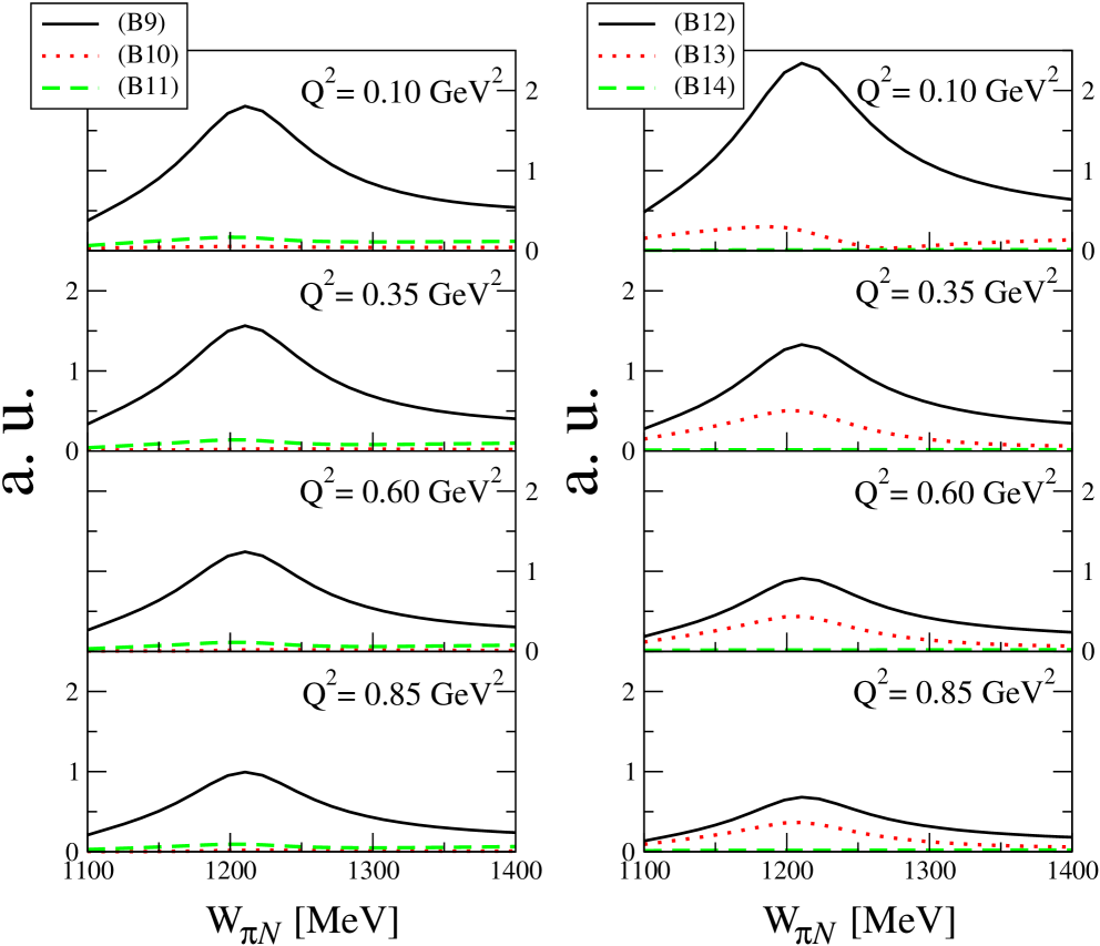
Figure 1: Modulus of the different vector (left panels) and axial (right panels) multipoles defined in Eqs. (64)-(69) of Appendix B. The scale is the same in all panels.

The relative $\Delta$background phases, $\Psi_{V}(\sqrt{s},q^{2})$ and $\Psi_{A}(\sqrt{s},q^{2})$, are fixed by requiring the phase of each of the amplitudes $\chi^{V}$ and $\chi^{A}$, defined as

$$\chi^{V} = \frac{1}{2}\left[(\chi_{1,1/2}-\chi_{-1,-1/2})+\sqrt{3}\ (\chi_{1,-1/2}-\chi_{-1,1/2})\right]$$ (30)

$$\chi^{A} = -\frac{1}{\sqrt{6}}\left[\sqrt{2}\ (\chi_{0,-1/2}+\chi_{0,1/2})+\sqrt{3}\ (\chi_{1,-1/2}+\chi_{-1,1/2})+(\chi_{1,1/2}+\chi_{-1,-1/2})\right]$$ (31)

to be $\delta_{P_{33}}(s)$. This is to say, we impose

$${\rm Im}\left[e^{-i\delta_{P_{33}}(s)}\chi^{V,A}\right]=0.$$ (32)

In each case, there exist two sets of solutions, which correspond to $\chi^{V,A}$ having phases $\delta_{P_{33}}$ and $(\delta_{P_{33}}+\pi)$, respectively (note that the $\pi N$ phase shift is defined up to a $\pi$ factor). We take the first set of solutions, because it leads to the smallest $\Psi_{V}$ and $\Psi_{A}$ Olsson extra phases. The second solution for the vector current is discarded by data on pion photoproduction off nucleons. This is shown in Fig. 2 where we apply the vector part of our model to describe the $\gamma p\to n\pi^{+}$ reaction. As seen from Fig. 2, a much better agreement with the data is obtained when taking the solution with the smallest $\Psi_{V}$ Olsson phase.

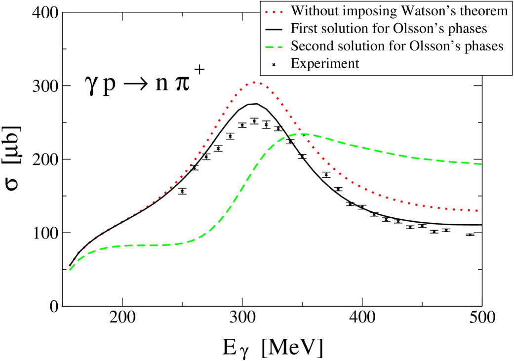
Figure 2: Results for the $\gamma p\to n\pi^{+}$ reaction obtained with the vector part of our model. A better description of the experimental data is obtained with the smallest $\Psi_{V}$ Olsson phase (first solution). Experimental data are taken from Ref. Fujii et al. (1977).

As for $\Psi_{A}$, the results shown in Fig. 12 of Appendix B of Ref. Hernandez et al. (2007) favor vector and axial $\Delta(1232)$ contributions having similar phases.

III Results and discussion

We (partially) unitarize the HNV model using Olsson’s implementation of Watson’s theorem discussed in Sec. II.3. For this purpose, we implement the constraints implicit in Eq. (32) using $\chi_{r,\lambda}$ amplitudes calculated by means of Eq. (22). In Appendix C, details on the evaluation of matrix elements $\langle\theta,\varphi;{0,\rho}|T(s)|0,0;{r,\lambda}\rangle$, which appears in Eq. (22), within the HNV model are provided. For the $P_{33}$ $\pi N$ phases we have used the output of the George Washington University Partial Wave Analysis(SAID) SAID from which we take the WI08 single energy values. In the analysis we neglect the influence of the small errors (ranging from 0.1% to 0.6%) in the $P_{33}$ phase shifts given in Ref. SAID .

III.1 Fit A

Following Ref. Hernandez et al. (2010), we make a simultaneous fit to both ANL and BNL data samples, taking into account deuterium effects, but now imposing the unitarity of the two dominant multipoles $\chi^{V,A}$. This analysis gives (fit A)

$$C_{5}^{A}(0)=1.12\pm 0.11,$$

$$M_{A\Delta}=(953.7\pm 62.6)\,{\rm MeV}.$$ (33)

The new central value of $C_{5}^{A}(0)$ agrees within 1$\sigma$ with the off-diagonal GTR prediction. As in Ref. Hernandez et al. (2010), the ANL Radecky et al. (1982) flux-averaged $d\sigma/dQ^{2}$ differential cross section, with a $W_{\pi N}=\sqrt{s}<1.4\,$GeV cut in the final pion-proton invariant mass, and the integrated cross sections for the three lowest neutrino energies (0.65, 0.9 and 1.1 GeV) of the BNL data set Kitagaki et al. (1986) have been fitted. A systematic error, due to flux uncertainties (20% for ANL and 10% for BNL data) has been added in quadratures to the statistical one.

In Table 1, we compare the results for $C_{5}^{A}(0)$ and $M_{A\Delta}$ obtained in this work with those from previous HNV fits carried out in Refs. Hernandez et al. (2007, 2010). With respect to the fit carried out in Ref. Hernandez et al. (2007), the consideration of BNL data and flux uncertainties in Ref. Hernandez et al. (2010) led to an increased value of $C_{5}^{A}(0)$, while strongly reducing the statistical correlations between $C_{5}^{A}(0)$ and $M_{A\Delta}$. The inclusion of background terms reduced $C_{5}^{A}(0)$, while deuteron effects slightly increased it by about 5%, consistently with the results of Refs. Hernandez et al. (2007) and Alvarez-Ruso et al. (1999); Graczyk et al. (2009). The implementation of Watson’s theorem, for the dominant vector and axial multipoles, in new fit A, further increases the $C_{5}^{A}(0)$ value, bringing it into much better agreement with the off-diagonal GTR prediction.

Table 1: Results from different fits to the ANL and BNL data. All fits include the ANL Radecky et al. (1982) flux-averaged $d\sigma/dQ^{2}$ differential cross section, with a $W_{\pi N}=\sqrt{s}<1.4\,$GeV cut, and the integrated cross sections for the three lowest neutrino energies (0.65, 0.9 and 1.1 GeV) of the BNL data set Kitagaki et al. (1986). Fits I^∗, II^∗ and IV are taken from Ref. Hernandez et al. (2010). In all cases Adler’s constraints ($C_{3}^{A}=0,\;C_{4}^{A}=-C_{5}^{A}/4$) Adler (1968); Bijtebier (1970) are imposed. Deuteron effects Hernandez et al. (2010) are included in fit IV and in those carried out in this work. The nonresonant chiral background contributions are included in all cases, with the exception of fit I^∗. For $C_{5}^{A}(q^{2})$ a dipole form, $C_{5}^{A}(q^{2})=C_{5}^{A}(0)/(1-q^{2}/M^{2}_{A\Delta})^{2}$, has been used in all fits except in the one carried out in Ref. Hernandez et al. (2007), where an extra factor $1/(1-q^{2}/3M_{A\Delta})$ was included [see Eq. (48) of that reference]. Finally, $r$ is the Gaussian correlation coefficient between $C_{5}^{A}(0)$ and $M_{A\Delta}$. For reference, the prediction of the GTR is $C_{5}^{A}(0)=1.15-1.2$.

	$C_{5}^{A}(0)$	$M_{A\Delta}$/GeV	Data	$r$	$\chi^{2}$/dof
Ref. Hernandez et al. (2007)	$0.867\pm 0.075$	$0.985\pm 0.082$	ANL	$-0.85$	0.40
Ref. Hernandez et al. (2010): Fit I∗ (only $\Delta$ pole)	$1.08\pm 0.10$	$0.92\pm 0.06$	ANL & BNL	$-0.06$	0.36
Fit II∗	$0.95\pm 0.11$	$0.92\pm 0.08$	ANL & BNL	$-0.08$	0.49
Fit IV (with deuteron effects)	$1.00\pm 0.11$	$0.93\pm 0.07$	ANL & BNL	$-0.08$	0.42
This work (unitarized + deuteron effects) fit A	$1.12\pm 0.11$	$0.954\pm 0.063$	ANL & BNL	$-0.08$	0.46

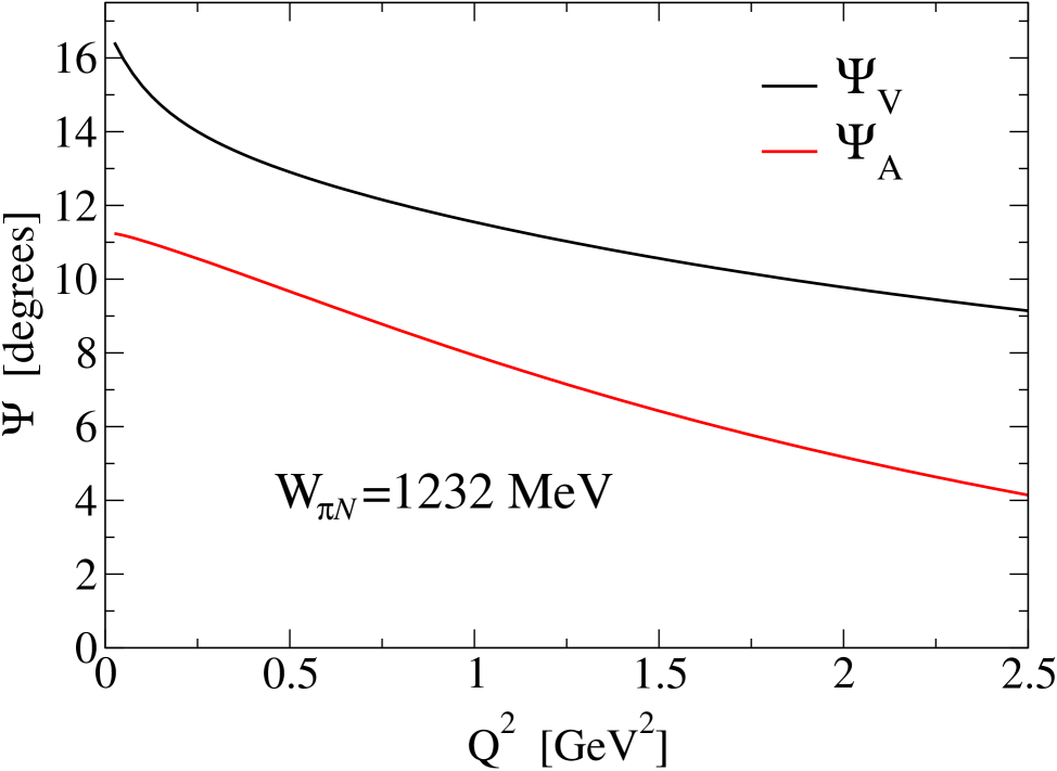
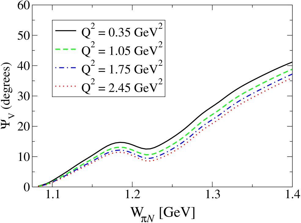
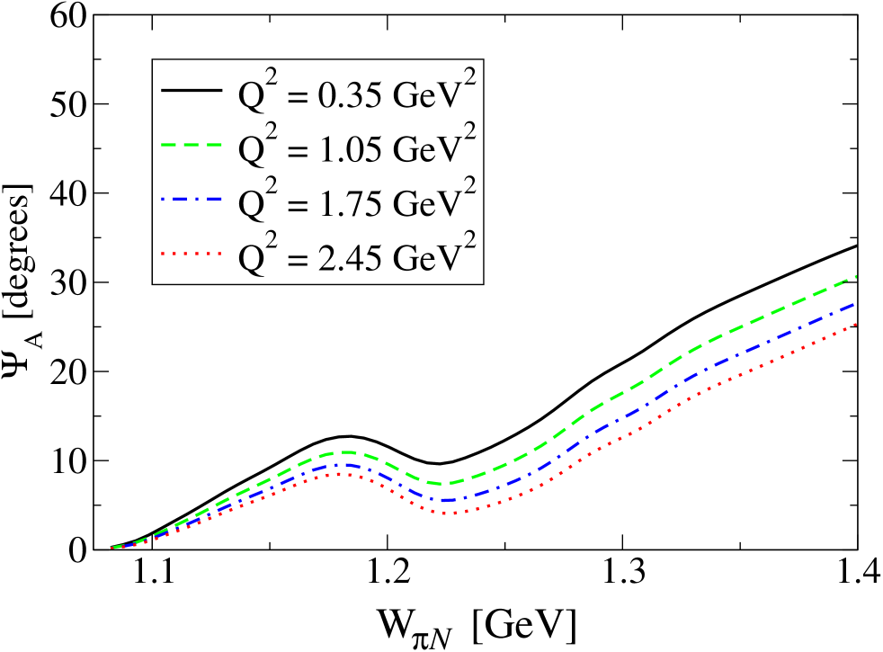
Figure 3: Olsson phases from fit A. Left panel: $\Psi_{V}$ and $\Psi_{A}$ at the $\Delta$ peak as a function of $Q^{2}=-q^{2}$. Middle and right panels: $\Psi_{V}$ and $\Psi_{A}$ as a function of the $\Delta$ invariant mass $W_{\pi N}$ for different $Q^{2}$ values, respectively.

The resulting Olsson phases from fit A are depicted in Fig. 3. In the left panel of Fig. 3 we show the phases $\Psi_{V},\Psi_{A}$ obtained at the $\Delta$ peak as a function of $Q^{2}$. In the middle and right panels of Fig. 3 we give, for different $Q^{2}$ values, the $\Psi_{V},\Psi_{A}$ dependence on the $\Delta$ invariant mass $W_{\pi N}$. The vector phase $\Psi_{V}$ agrees reasonably well with the one determined for electron scattering in Ref. Gil et al. (1997).

The results of the (partially) unitarized model derived in this work (fit A) are confronted to the fitted data in Fig. 4. The same good agreement to the data as in Ref. Hernandez et al. (2010), where partial unitarity was not imposed, is now obtained with a higher $C_{5}^{A}(0)$ consistent with the GTR. The increase in the $C_{5}^{A}(0)$ value with respect to that calculation is compensated by the change in the interference between the dominant $\Delta$ term and the background terms once Watson’s theorem is imposed on the dominant multipoles.

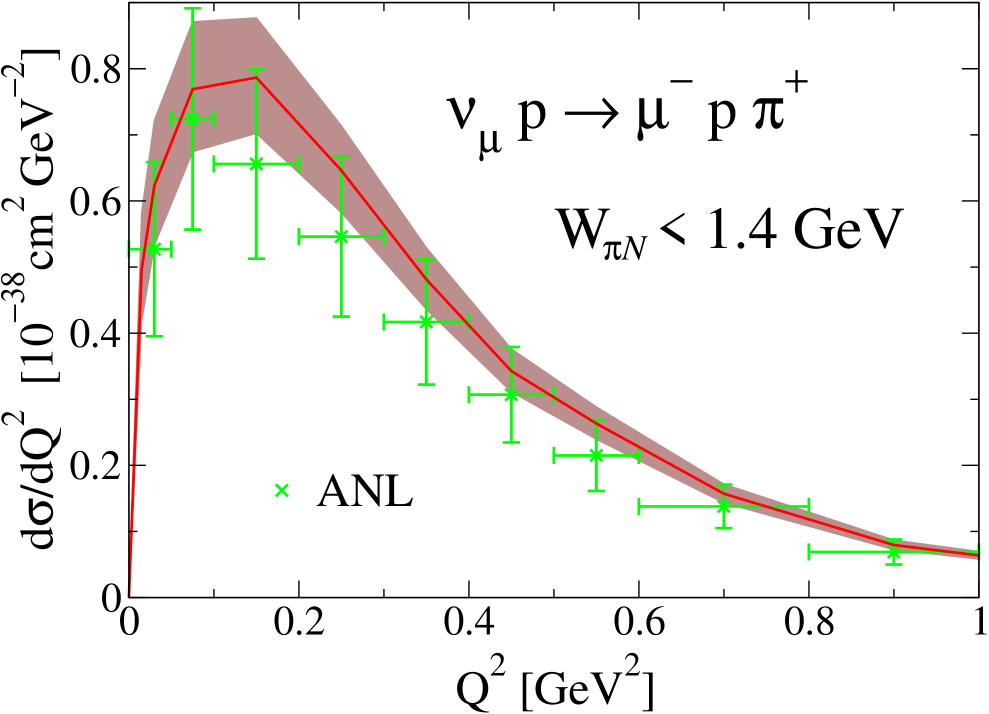
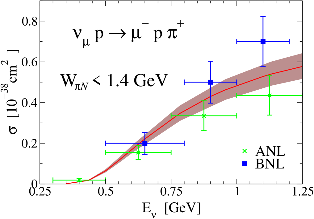
Figure 4: Results from fit A for the differential $d\sigma/dQ^{2}$ (left) and total (right) cross section for the $\nu_{\mu}p\to\mu^{-}p\pi^{+}$ reaction compared to the ANL Radecky et al. (1982) and BNL Kitagaki et al. (1986) data. The theoretical bands correspond to the variation of the results when $C_{5}^{A}(0)$ changes within the error interval determined from the fit. Experimental data include a systematic error, due to flux uncertainties (20% for ANL and 10% for BNL data), which has been added in quadratures to the statistical ones. Theoretical results and ANL data include a cut in the final pion-proton invariant mass given by $W_{\pi N}<1.4\,$GeV. Deuteron effects have been taken into account assuming that the neutron in the deuteron acts as a spectator (details in Ref. Hernandez et al. (2010)).

In Fig. 5 we show the predictions of the partially unitarized (Fit A) HNV model for the $\nu_{\mu}n\to\mu^{-}p\pi^{0}$ and $\nu_{\mu}n\to\mu^{-}n\pi^{+}$ channels. They are compared to the ANL and BNL data, assuming that the proton in the deuteron acts as a spectator. The problem with the $\nu_{\mu}n\to\mu^{-}n\pi^{+}$ channel, where data are underestimated in most theoretical models, still persists after partial unitarization. This significant discrepancy deserves additional work, even more so because there exist only two independent amplitudes, and thus the $p\pi^{0}$ and $p\pi^{+}$ channels fully determine the $n\pi^{+}$ amplitude Hernandez et al. (2007). We would like to point out that the crossed $\Delta$ mechanism has a large contribution in the $n\pi^{+}$ channel. Indeed, besides the $\Delta$ propagator, the numerical factors of the (direct and crossed) $\Delta$ mechanisms are $(\sqrt{3}~{}\&~{}1/\sqrt{3})$, $(2/\sqrt{3}~{}\&~{}-2/\sqrt{3})$ and $(1/\sqrt{3}~{}\&~{}\sqrt{3})$ for the $p\pi^{+}$, $p\pi^{0}$ and $n\pi^{+}$ channels, respectively Hernandez et al. (2007). The spin structure of the $\Delta$ propagator used in Ref. Hernandez et al. (2007) suffers from some off-shell ambiguities/inconsistencies, which are clearly enhanced in the evaluation of the crossed term, where the resonance is far from its mass shell. This might have consequences, which would affect much more the $n\pi^{+}$ channel than the other two charge configurations. Research along these lines is underway.

Effects of the final state interactions (FSIs) on cross sections for the single pion production off the deuteron should also be considered and might help to explain the puzzling $n\pi^{+}$ channel. Such effects have been recently examined in the work of Ref. Wu et al. (2015). There, it is found that the orthogonality between the deuteron and final $pn$ scattering wave functions significantly reduces the cross sections. Thus the ANL and BNL data on the deuterium target might need a more careful analysis with the FSIs taken into account. It is also relevant to incorporate the kinematical cuts implemented in the experiments to properly separate the three reaction channels.

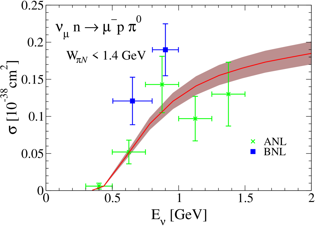
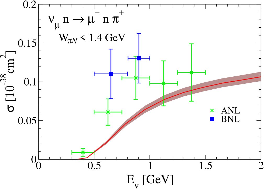
Figure 5: Results from fit A [Eq. (33)] for the $\nu_{\mu}n\to\mu^{-}p\pi^{0}$ (left panel) and $\nu_{\mu}n\to\mu^{-}n\pi^{+}$ (right panel) total cross sections as compared to ANL Radecky et al. (1982) and BNL Kitagaki et al. (1986) data. Theoretical bands and experimental errors have the same meaning as in Fig. 4. Theoretical results and ANL data include a cut in the final active nucleon-pion invariant mass given by $W_{\pi N}<1.4\,$GeV. Deuteron effects have been taken into account as explained in Ref. Hernandez et al. (2010), assuming that the proton in the deuteron acts as a spectator.

Finally, in Fig. 6 we give the fit A results for the $\bar{\nu}_{\mu}n\to\mu^{+}n\pi^{-}$ and $\nu_{\mu}n\to\nu_{\mu}p\pi^{-}$ channels. In the first case we compare with the data from Ref. Bolognese et al. (1979) that were obtained at the CERN proton synchroton (PS) using a freon-propane ($\rm CF_{3}Br-C_{3}H_{8}$) target. There is a large discrepancy in this case between the theoretical calculation and the experimental data. As shown in Ref. Athar et al. (2007), this can be explained by nuclear medium and pion absorption effects, which were not properly taken into account in the analysis of Ref. Bolognese et al. (1979). For the second reaction, we find a nice agreement with the experimental data from Ref. Derrick et al. (1980).

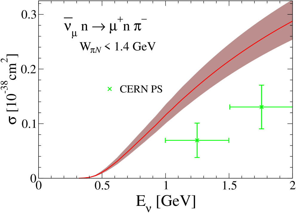
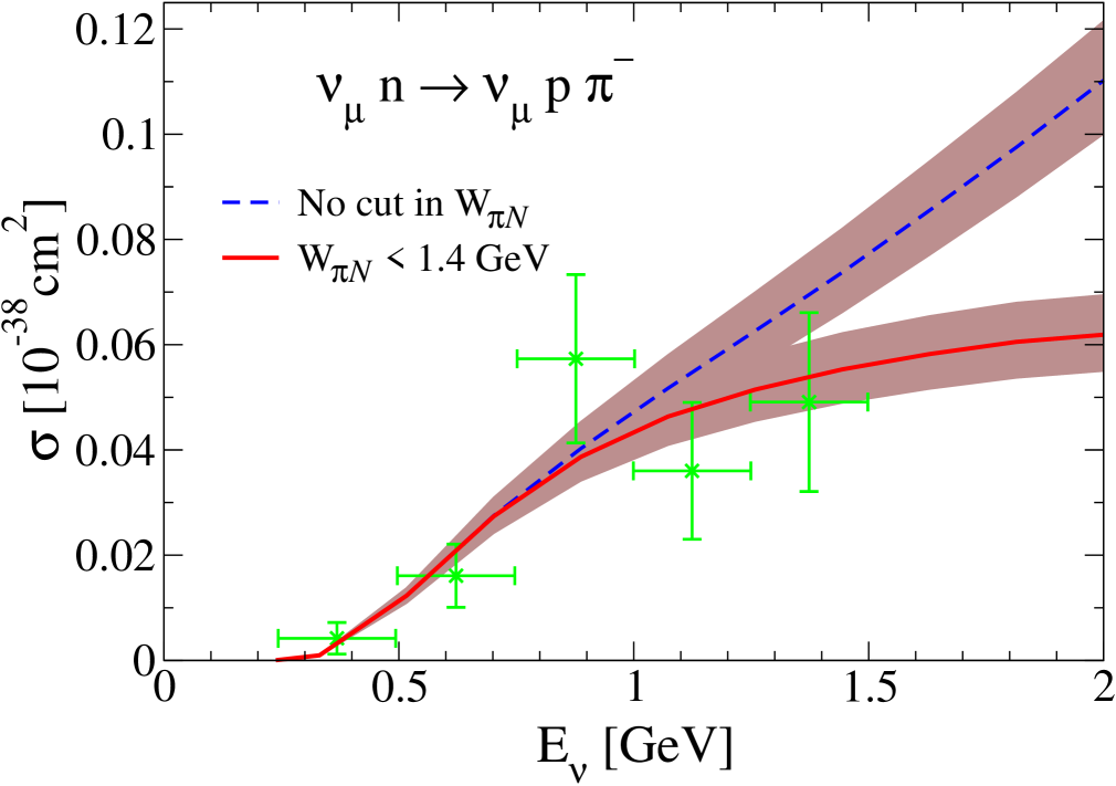
Figure 6: Results from fit A [Eq. (33)] for the $\bar{\nu}_{\mu}n\to\mu^{+}n\pi^{-}$ (left panel) and $\nu_{\mu}n\to\nu_{\mu}p\pi^{-}$ (right panel) total cross sections. Data from CERN PS were taken in a freon-propane ($\rm CF_{3}Br-C_{3}H_{8}$) target Bolognese et al. (1979). Experimental data for the $\nu_{\mu}n\to\nu_{\mu}p\pi^{-}$ reaction are from Ref. Derrick et al. (1980). Since this latter cross section was measured at ANL, we have assumed a 20% systematic error, due to flux uncertainties, that has been added in quadratures to the statistical error. Besides, for the $\nu_{\mu}n\to\nu_{\mu}p\pi^{-}$ case, we have taken into account deuteron effects, as explained in Ref. Hernandez et al. (2010), assuming the proton in the deuteron as a spectator. Theoretical bands have the same meaning as in Fig. 4. Theoretical results, except where indicated, include a cut in the final pion-nucleon invariant mass given by $W_{\pi N}<1.4\,$GeV.

III.2 Fit B

The ANL and BNL bubble chamber pion production measurements have been recently revisited Wilkinson et al. (2014). Both experiments have been reanalyzed to produce the ratio between the $\sigma(\nu_{\mu}p\to\mu^{-}p\pi^{+})$ and the charged current quasielastic (CCQE) cross sections measured in deuterium, cancelling in this way the flux uncertainties present in the data. A good agreement between the two experiments for these ratios was found, providing in this way an explanation to the longstanding tension between the two data sets. By multiplying the cross section ratio by the theoretical CCQE cross section on the deuteron, which is well under control, flux normalization independent pion production cross sections were extracted. We have taken advantage of these developments and performed a new fit considering some of the new data points.

We have minimized

$$\chi^{2}=\sum_{i\in{\rm ANL}}\left(\frac{\beta d\sigma/dQ_{i}^{2}|_{\rm exp}-d\sigma/dQ_{i}^{2}|_{\rm th}}{\beta\Delta(d\sigma/dQ_{i}^{2}|_{\rm exp})}\right)^{2}+\sum_{i\in{\rm ANL}}\left(\frac{\sigma_{i}|_{\rm exp}-\sigma_{i}|_{\rm th}}{\Delta(\sigma_{i}|_{\rm exp})}\right)^{2}+\sum_{i\in{\rm BNL}}\left(\frac{\sigma_{i}|_{\rm exp}-\sigma_{i}|_{\rm th}}{\Delta(\sigma_{i}|_{\rm exp})}\right)^{2}\,.$$ (34)

The ANL and BNL integrated cross sections included in the above $\chi^{2}$, taken from Ref. Wilkinson et al. (2014), are collected in Table 2.

Table 2: ANL and BNL integrated cross sections (in units of $10^{-38}$ cm²) taken from the reanalysis of Ref. Wilkinson et al. (2014) and included in the $\chi^{2}$ of Eq. (34) (fit B).

$E_{\nu}$ (GeV)	$\sigma|_{\rm exp}$	$\Delta(\sigma|_{\rm exp})$	Exp.
0.3	0.0020	0.0020	ANL
0.5	0.070	0.012	ANL
0.7	0.28	0.03	ANL
0.9	0.50	0.06	ANL
0.5	0.056	0.016	BNL
0.7	0.26	0.03	BNL
0.9	0.43	0.04	BNL

Since no cut in the outgoing pion-nucleon invariant mass was considered in the new analysis of Ref. Wilkinson et al. (2014), and in order to avoid heavier resonances from playing a significant role, we have only included data points corresponding to laboratory neutrino energies $E_{\nu}\leq 1.1$ GeV. To constrain the $q^{2}$ dependence, we have also fitted the shape of the original ANL flux-folded $d\sigma/dQ^{2}$ distribution, not affected by the new analysis of Ref. Wilkinson et al. (2014), where a $W_{\pi N}=\sqrt{s}<1.4\,$GeV cut in the final pion-proton invariant mass was implemented. The new best fit parameter $\beta$ in the first term of Eq. (34) is an arbitrary scale that allows us to consider only the shape of this distribution. In turn, we do not now include any systematic error on the ANL $d\sigma/dQ^{2}$ differential cross section. As in fit A, we consider deuterium effects and Adler’s constraints ($C_{3}^{A}=0,\;C_{4}^{A}=-C_{5}^{A}/4$) on the axial form factors and for $C_{5}^{A}(q^{2})$ use the dipole functional form shown in the caption of Table 1. Besides, Olsson’s approximate implementation of Watson’s theorem is also taken into account. The best fit parameters in this case (fit B) are

$$C_{5}^{A}(0) = 1.14\pm 0.07,$$

$$M_{A\Delta} = (959.4\pm 66.9)\,{\rm MeV},$$ (35)

with $\beta=1.19\pm 0.08$ and $\chi^{2}/dof=0.3$. The values for $C_{5}^{A}(0)$ and $M_{A}$ from fit B are very close to the ones obtained in fit A. Without including the Olsson phases, fit B gives a smaller $C_{5}^{A}(0)=1.05\pm 0.07$ value, in worse agreement with the GTR prediction. This is the same effect seen when comparing fit A with fit IV in Ref. Hernandez et al. (2010). The value $\beta=1.19\pm 0.08$ suggests that ANL results in Ref. Radecky et al. (1982) could have underestimated the pion production cross sections by some $20\%$ due to neutrino flux uncertainties. A comparison of the theoretical results from fit B and the fitted data is now shown in Fig. 7. Similar results to those from fit A are obtained for the Olsson phases and the cross sections for the other channels.

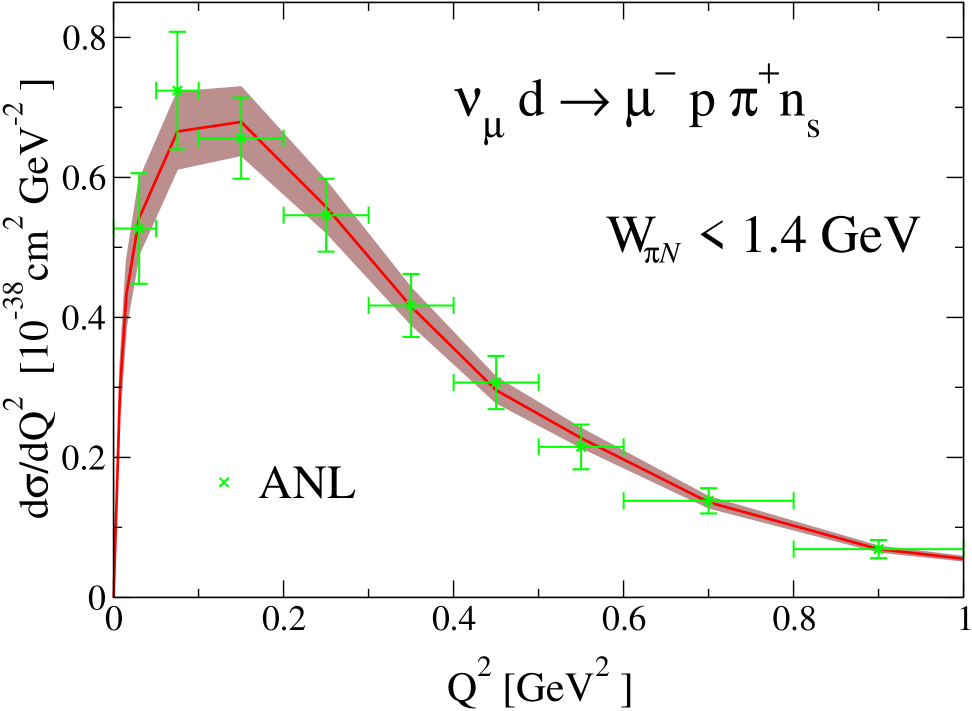
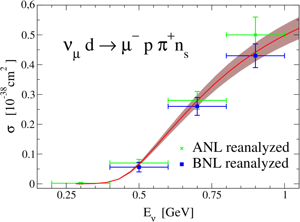
Figure 7: Results from fit B [Eq. (35)] for the shape of the differential $d\sigma/dQ^{2}$ (left) and for total cross sections (right) for the $\nu_{\mu}p\to\mu^{-}p\pi^{+}$ reaction compared , respectively, to the ANL Radecky et al. (1982) data and the ANL and BNL reanalyzed total cross sections of Ref. Wilkinson et al. (2014). Theoretical bands are as in Fig. 4. In the left panel, both experimental data and theoretical results include a cut in the final pion-neutron invariant mass given by $W_{\pi N}<1.4\,$GeV. Besides, theoretical results in the left panel have been divided by $\beta=1.19$, accounting for flux uncertainties [see Eq.(34)]. Deuteron effects have been taken into account as explained in Ref. Hernandez et al. (2010).

IV Final remarks

Pion production on deuteron target induced by neutrinos and antineutrinos has been studied using the HNV model Hernandez et al. (2007), which takes into account nonresonant amplitudes, required by chiral symmetry, as well as resonant ones with $\Delta(1232)$ and $N^{*}(1520)$ intermediate states. Phenomenological form factors allow us to apply the model to finite 4-momentum transfers $q^{2}$ probed in neutrino experiments. The model has now been improved by imposing Watson’s theorem to the dominant vector and axial multipoles. In this way, unitarity has been partially restored.

With this theoretical tool we have undertaken a new determination of the leading axial $N\Delta(1232)$ transition form factor from ANL and BNL data. We have fitted not only the original data (fit A) but also those obtained in a recent reanalysis Wilkinson et al. (2014) that has removed the tension between the two data sets by considering flux independent ratios (fit B). Both fits A and B show that the partial unitarization increases the value of the leading axial coupling $C_{5}^{A}(0)$ with respect to fits where no unitarization was applied. Thanks to the new analysis of Ref. Wilkinson et al. (2014), the error in $C_{5}^{A}(0)$ has been reduced from 10% (fit A) to 6% (fit B). The agreement with the data is equally satisfactory as in previous fits performed without unitarization, but the new $C_{5}^{A}(0)$ values are in better agreement with the prediction from the off-diagonal GTR. One should also mention that the description of pion photoproduction at the $\Delta(1232)$ peak is also improved without refitting the electromagnetic couplings (Fig. 2). It is the new interference pattern between the $\Delta$-pole amplitude and background contributions that compensates for the increase in the $C_{5}^{A}(0)$ value. Actually, the results are compatible with the ones obtained in a simpler model where only the dominant $\Delta$ mechanism was included and where $C_{5}^{A}(0)\approx 1.15-1.2$, as given by the off-diagonal GTR. However, a more complete model containing not only the $\Delta$ mechanism but also background terms is definitely more robust. In fact, as shown in Ref. Hernandez et al. (2007), there are parity violating observables that are nonzero only in the presence of background terms.

Full unitarity is also to be preferred. The advantage of the simpler scheme adopted here resides mostly in its simplicity. This would allow for an easier implementation in event generators used in the analysis of neutrino experiments while, at the same time, providing an accurate description of the pion production data for $W_{\pi N}<1.4\,$GeV. The framework is also general enough to correct for deviations from Watson’s theorem in more elaborated weak pion production models. The accuracy can be also increased by fixing the phases in other subdominant multipoles.

Appendix A CM two-particle helicity states

We follow the notation in Ref. Martin and Spearman (1970), up to some trivial factors in the normalization of the states. Particle states are defined by the Poincaré symmetry group Casimir operators. Thus, the states $|m,j,\vec{p},\lambda\rangle$ are characterized by the mass ($m$), spin ($j$), 3-momentum ($\vec{p}$ ) and helicity ($\lambda$) of the particle. They are constructed as

$$|m,j;\vec{p},\lambda\rangle=R(\varphi,\theta,-\varphi)Z_{|\vec{p}\,|}|m,j;\vec{0},\lambda\rangle\,,$$ (36)

with $Z_{|\vec{p}\,|}$ being a boost in the positive $z$ direction and $R(\varphi,\theta,-\varphi)$ a rotation that takes that axis into the direction of $\vec{p}$ ($\theta,\varphi$ are the polar and azimuthal angles of $\vec{p}$, $0\leq\theta\leq\pi$, $0\leq\varphi<2\pi$). The state $|\vec{0},\lambda\rangle$ has $\vec{p}=\vec{0}$ and spin projection along the Z axis $\lambda$. After the transformations, $\lambda$ becomes the helicity of the one-particle state. The normalization is such that

$$\langle m,j,\vec{p},\lambda|m,j,\vec{p}^{\,\prime},\lambda^{\prime}\rangle=(2\pi)^{3}2E(\vec{p}\,)\delta^{3}(\vec{p}-\vec{p}^{\,\prime})\delta_{\lambda\lambda^{\prime}}$$ (37)

with $E(\vec{p}\,)=\sqrt{m^{2}+\vec{p}^{\,2}}$. Helicity CM two-particle states are defined as

$$|p,\theta,\varphi;\lambda_{1},\lambda_{2};\gamma\,\rangle=|m_{1},j_{1};\vec{p},\lambda_{1}\rangle\otimes\overline{|m_{2},j_{2};-\vec{p},\lambda_{2}\rangle}\,,$$ (38)

where $\gamma$ encompasses all other not explicitly identified quantum numbers, and

$$\overline{|m_{2},j_{2};-\vec{p},\lambda_{2}\rangle}=(-1)^{j_{2}-\lambda_{2}}R(\varphi,\theta,-\varphi)R(0,\pi,0)Z_{|\vec{p}\,|}|m_{2},j_{2};\vec{0},\lambda_{2}\rangle\,;$$ (39)

the phase factor $(-1)^{j_{2}-\lambda_{2}}$ is introduced so that as $\vec{p}\to 0$

$$\overline{|m_{2},j_{2};\vec{p}=\vec{0},\lambda_{2}\rangle}=|m_{2},j_{2};\vec{p}=\vec{0},-\lambda_{2}\rangle$$ (40)

Defining the two-particle state in this way guarantees good transformation properties under rotations

$$|p,\theta,\varphi;\lambda_{1},\lambda_{2};\gamma\,\rangle=R(\varphi,\theta,-\varphi)|p,0,0;\lambda_{1},\lambda_{2};\gamma\,\rangle.$$ (41)

It is convenient to decompose

$$|p,\theta,\varphi;\lambda_{1},\lambda_{2};\gamma\,\rangle=2\pi\sqrt{\frac{4\sqrt{s}}{|\vec{p}\,|}}\,|P\rangle\,|\theta,\varphi;\lambda_{1},\lambda_{2};\gamma\,\rangle,$$ (42)

with $P$ the total four-momentum and $P^{2}=s$. The normalizations are

$$\langle P^{\prime}|P\rangle = (2\pi)^{4}\delta^{4}(P-P^{\prime}),$$

$$\langle\theta^{\prime},\varphi^{\prime};\lambda^{\prime}_{1},\lambda^{\prime}_{2};\gamma\,^{\prime}\,|\theta,\varphi;\lambda_{1},\lambda_{2};\gamma\,\rangle = \delta(\Omega-\Omega^{\prime})\delta_{\lambda_{1}\lambda^{\prime}_{1}}\delta_{\lambda_{2}\lambda^{\prime}_{2}}\delta_{\gamma\gamma\,^{\prime}}.$$ (43)

The decomposition in Eq. (42) attends to the fact the $4$-momentum is a conserved quantity and thus

$$\langle F|S|I\rangle=(2\pi)^{4}\delta^{4}(P_{F}-P_{I})\langle\alpha_{F}|S_{P}|\alpha_{I}\rangle$$ (44)

and any state of the Hilbert space, containing any number of particles, can be written as a superposition of vectors of the form $|P\rangle\,|\alpha\rangle$. The set of vectors $|\alpha\rangle$ spans the so-called little Hilbert space Martin and Spearman (1970). It follows that the scattering operator $S$ may be written as the direct product

$$S=\mbox{1}\rule{0.28453pt}{6.45831pt}\hskip 4.30554pt\otimes S_{P}$$ (45)

such that

$$\langle F|S|I\rangle=\langle P_{F}|\mbox{1}\rule{0.28453pt}{6.45831pt}\hskip 4.30554pt|P_{I}\rangle\langle\alpha_{F}|S_{P}|\alpha_{I}\rangle$$ (46)

Just as in the case of the $S$ operator, $T$ may also be written as a direct product

$$T=\mbox{1}\rule{0.28453pt}{6.45831pt}\hskip 4.30554pt\otimes T_{P},\qquad S_{P}=\mbox{1}\rule{0.28453pt}{6.45831pt}\hskip 4.30554pt-iT_{P}$$ (47)

This is the form in which the $T$ matrix is generally used. In fact we refer to $T_{P}$ as the $T$ operator and $T_{FI}(s)=\langle\alpha_{F}|T_{P}|\alpha_{I}\rangle$ as the $T-$matrix element.

The CM states can be written in terms of states with well-defined total angular momentum

$$|p,J,M;\lambda_{1},\lambda_{2};\gamma\,\rangle=2\pi\sqrt{\frac{4\sqrt{s}}{|\vec{p}\,|}}\,|P\rangle\,|J,M;\lambda_{1},\lambda_{2};\gamma\,\rangle,$$ (48)

with

$$\langle J^{\prime},M^{\prime};\lambda^{\prime}_{1},\lambda^{\prime}_{2};\gamma\,^{\prime}\,|J,M;\lambda_{1},\lambda_{2};\gamma\,\rangle=\delta_{JJ^{\prime}}\delta_{MM^{\prime}}\delta_{\lambda_{1}\lambda^{\prime}_{1}}\delta_{\lambda_{2}\lambda^{\prime}_{2}}\delta_{\gamma\gamma\,^{\prime}}.$$ (49)

Starting from the case $\theta=0,\varphi=0$

$$|0,0;\lambda_{1},\lambda_{2};\gamma\,\rangle=\sum_{J}C_{J}\,|J,J_{z}=\lambda;\lambda_{1},\lambda_{2};\gamma\,\rangle,$$ (50)

with $\lambda=\lambda_{1}-\lambda_{2}$, one arrives at

$$|\theta,\varphi;\lambda_{1},\lambda_{2};\gamma\,\rangle=\sum_{J,M}C_{J}\,{\cal D}^{(J)}_{M\lambda}(\varphi,\theta,-\varphi)\,|J,M;\lambda_{1},\lambda_{2};\gamma\,\rangle,\ \ \lambda=\lambda_{1}-\lambda_{2},$$ (51)

where ${\cal D}^{(J)}_{MM^{\prime}}(\alpha,\beta,\gamma)$ is the matrix representation of a rotation operator $R(\alpha,\beta,\gamma)$ in an irreducible representation space,

$${\cal D}^{(J)}_{M^{\prime}M}(\alpha,\beta,\gamma)=e^{-i\alpha M^{\prime}}d^{J}_{M^{\prime}M}(\beta)\,e^{-i\gamma M},\qquad d^{J}_{M^{\prime}M}(\beta)=\langle JM^{\prime}|e^{-i\beta J_{y}}|JM\rangle$$ (52)

From the above equation and using that

$$\int d\Omega\,{\cal D}^{(J)*}_{M\lambda}(\varphi,\theta,-\varphi){\cal D}^{(J^{\prime})}_{M^{\prime}\lambda}(\varphi,\theta,-\varphi)=\frac{4\pi}{2J+1}\delta_{JJ^{\prime}}\delta_{MM^{\prime}}$$ (53)

it follows that

$$|J,M;\lambda_{1},\lambda_{2};\gamma\,\rangle = \frac{2J+1}{4\pi\,C_{J}}\int d\Omega\ {\cal D}^{(J)*}_{M\lambda}(\varphi,\theta,-\varphi)\,|\theta,\varphi;\lambda_{1},\lambda_{2};\gamma\,\rangle$$ (54)

$$= \sqrt{\frac{2J+1}{4\pi}}\int d\Omega\ {\cal D}^{(J)*}_{M\lambda}(\varphi,\theta,-\varphi)\,|\theta,\varphi;\lambda_{1},\lambda_{2};\gamma\,\rangle,\ \ \lambda=\lambda_{1}-\lambda_{2}\,,$$

where we have made use of the normalization conditions to determine $|C_{J}|^{2}=\frac{2J+1}{4\pi}$ and have taken the coefficients $C_{J}$ to be real. States with well-defined orbital angular momentum $L$ and spin $S$ can be introduced as

$$|J,M;\lambda_{1},\lambda_{2};\gamma\,\rangle = \sum_{L,S}\sqrt{\frac{2L+1}{2J+1}}(L,S,J|0,\lambda,\lambda)(j_{1},j_{2},S|\lambda_{1},-\lambda_{2},\lambda)|J,M;L,S;\gamma\,\rangle,$$

$$|J,M;L,S;\gamma\,\rangle = \sum_{\lambda_{1},\lambda_{2}}\sqrt{\frac{2L+1}{2J+1}}(L,S,J|0,\lambda,\lambda)(j_{1},j_{2},S|\lambda_{1},-\lambda_{2},\lambda)|J,M;\lambda_{1},\lambda_{2};\gamma\,\rangle,$$ (55)

where $(j_{1},j_{2},j|m_{1},m_{2},M)$ are the Clebsch-Gordan coefficients and $\lambda=\lambda_{1}-\lambda_{2}$ as usual.

Appendix B Properties of the $\chi_{r,\lambda}$ amplitudes defined in Eq. (21)

The $\chi_{r,\lambda}$ amplitudes in Eq. (21) can be rewritten in terms of states $|J,M;L,S\rangle$ with well-defined total orbital ($L$) and spin ($S$) angular momenta as

$$\chi_{r,\lambda} = \sqrt{\frac{3}{8}}\sum_{\rho}(1,1/2,3/2|0,-\rho,-\rho)\,\langle 3/2,M;{0,\rho}|T(s)|3/2,M;{r,\lambda}\rangle$$ (56)

$$= \frac{1}{\sqrt{2}}\langle 3/2,M;{L=1,S=1/2}|T(s)|3/2,M;{r,\lambda}\rangle$$

$$= \sum_{L^{\prime},S^{\prime}}\sqrt{\frac{2L^{\prime}+1}{8}}(1,1/2,S^{\prime}|r,-\lambda,M)(L^{\prime},S^{\prime},3/2|0,M,M)\langle{L=1,S=1/2}|T_{J=\frac{3}{2}}(s)|{L^{\prime}S^{\prime}}\rangle,$$

with $M=r-\lambda$. Note that the matrix element of the $T$ scattering operator does not depend on $M$, since it is invariant under rotations. Now, the amplitude has a vector and an axial part,

$${T}={T}^{V}-{T}^{A},$$ (57)

and under a parity transformation, we have

$${\cal P}\,{T}\,{\cal P}^{\dagger} = {T}^{V}+T^{A}$$ (58)

$${\cal P}|J,M;LS\rangle = \eta_{1}\eta_{2}(-1)^{L}|J,M;L,S\rangle$$ (59)

where $\eta_{1,2}$ are the intrinsic parities of the particles (1 for nucleons and $-1$ for $\pi$ and $W$). We thus find that only odd (even) $L^{\prime}$ waves contribute to the vector (axial) part of the $\chi_{r,\lambda}$,

$$\chi_{r,\lambda} = \chi_{r,\lambda}^{V}-\chi_{r,\lambda}^{A}$$ (60)

$$\chi_{r,\lambda}^{V} = \sum_{S^{\prime}=1/2,3/2}\sum_{L^{\prime}=1,3}\sqrt{\frac{2L^{\prime}+1}{8}}(1,1/2,S^{\prime}|r,-\lambda,M)(L^{\prime},S^{\prime},3/2|0,M,M)\langle{L=1,S=1/2}|T^{V}_{J=\frac{3}{2}}(s)|{L^{\prime}S^{\prime}}\rangle$$ (61)

$$\chi_{r,\lambda}^{A} = \sum_{S^{\prime}=1/2,3/2}\sum_{L^{\prime}=0,2}\sqrt{\frac{2L^{\prime}+1}{8}}(1,1/2,S^{\prime}|r,-\lambda,M)(L^{\prime},S^{\prime},3/2|0,M,M)\langle{L=1,S=1/2}|T^{A}_{J=\frac{3}{2}}(s)|{L^{\prime}S^{\prime}}\rangle$$ (62)

Now taking into account

$$(1,1/2,S^{\prime}|r,-\lambda,M)(L^{\prime},S^{\prime},3/2|0,M,M)=(-1)^{L^{\prime}}(1,1/2,S^{\prime}|-r,\lambda,-M)(L^{\prime},S^{\prime},3/2|0,-M,-M)$$ (63)

we trivially find Eq. (27).

On the other hand, using the basis introduced in Eq. (28), we obtain the following relations

$$-\frac{1}{2}\left\langle L=1,S=1/2\,|T^{V}_{J=3/2}|L^{\prime}=1,\tilde{l}=1\right\rangle = \frac{1}{2}\left(\chi^{V}_{1,1/2}+\sqrt{3}\chi^{V}_{1,-1/2}\right),\,[M_{1+}]$$ (64)

$$-\frac{1}{2}\left\langle L=1,S=1/2\,|T^{V}_{J=3/2}|L^{\prime}=1,\tilde{l}=2\right\rangle = \frac{1}{\sqrt{20}}\left(2\sqrt{2}\chi^{V}_{0,-1/2}+\sqrt{3}\chi^{V}_{1,-1/2}-3\chi^{V}_{1,1/2}\right),\,[E_{1+}/L_{1+}]$$ (65)

$$-\frac{1}{2}\left\langle L=1,S=1/2\,|T^{V}_{J=3/2}|L^{\prime}=3,\tilde{l}=2\right\rangle = \frac{1}{\sqrt{10}}\left(-\sqrt{6}\chi^{V}_{0,-1/2}+\chi^{V}_{1,-1/2}-\sqrt{3}\chi^{V}_{1,1/2}\right),\,[E_{1+}/L_{1+}]$$ (66)

$$-\frac{1}{2}\left\langle L=1,S=1/2\,|T^{A}_{J=3/2}|L^{\prime}=0,\tilde{l}=1\right\rangle = -\frac{1}{\sqrt{6}}\left(\sqrt{2}\chi^{A}_{0,-1/2}+\sqrt{3}\chi^{A}_{1,-1/2}+\chi^{A}_{1,1/2}\right)$$ (67)

$$-\frac{1}{2}\left\langle L=1,S=1/2\,|T^{A}_{J=3/2}|L^{\prime}=2,\tilde{l}=1\right\rangle = -\frac{1}{\sqrt{12}}\left(-2\sqrt{2}\chi^{A}_{0,-1/2}+\sqrt{3}\chi^{A}_{1,-1/2}+\chi^{A}_{1,1/2}\right)$$ (68)

$$-\frac{1}{2}\left\langle L=1,S=1/2\,|T^{A}_{J=3/2}|L^{\prime}=2,\tilde{l}=2\right\rangle = -\frac{1}{2}\left(\chi^{A}_{1,-1/2}-\sqrt{3}\chi^{A}_{1,1/2}\right)$$ (69)

Appendix C Computation of the $\chi_{r,\lambda}(s)$ amplitudes within the HNV model

Equation (22) allows us to compute $\chi_{r,\lambda}(s)$ in terms of the matrix elements $\underbrace{\langle\theta,\varphi;{0,\rho}}_{\pi^{+}p}|T(s)|\underbrace{0,0;{r,\lambda}\rangle}_{W^{+}p}$, which involve the helicity CM two-particle states introduced in Eq. (38). We have always labeled the proton as the second particle. This is to say that the “bar” $\overline{|j;-\vec{p},\lambda\rangle}$ states correspond to the protons. One can prove that

$$\overline{|j;-\vec{p},\lambda\rangle}=(-1)^{j-\lambda}(-1)^{2j}e^{-2i\lambda\varphi}|j;-\vec{p},\lambda\rangle$$ (70)

with

$$|j;-\vec{p},\lambda\rangle=R(\varphi+\pi,\pi-\theta,-\varphi-\pi)Z_{|\vec{p}\,|}|j;\vec{0},\lambda\rangle,$$ (71)

where $\theta$ and $\varphi$ are the polar and azimuthal angles of $\vec{p}$. The latter states, $|j;-\vec{p},\lambda\rangle$ for the case of a nucleon $j=1/2$, can be easily obtained using the Dirac space representations of the boost and the rotation that appears in Eq. (71). Finally, and using Eq. (70), we find that the spinors corresponding to the bar states are

$$\overline{\left.\Big{|}-\vec{p},\lambda=1/2\right\rangle} \equiv \sqrt{E+M_{N}}\left(\begin{array}[]{c}-\sin\frac{\theta}{2}e^{-i\varphi}\\ \cos\frac{\theta}{2}\\ -\frac{|\vec{p}\,|}{E+M_{N}}\sin\frac{\theta}{2}e^{-i\varphi}\\ \frac{|\vec{p}\,|}{E+M_{N}}\cos\frac{\theta}{2}\end{array}\right)$$ (76)

$$\overline{\left.\Big{|}-\vec{p},\lambda=-1/2\right\rangle} \equiv \sqrt{E+M_{N}}\left(\begin{array}[]{c}\cos\frac{\theta}{2}\\ \sin\frac{\theta}{2}e^{i\varphi}\\ -\frac{|\vec{p}\,|}{E+M_{N}}\cos\frac{\theta}{2}\\ -\frac{|\vec{p}\,|}{E+M_{N}}\sin\frac{\theta}{2}e^{i\varphi}\end{array}\right)$$ (81)

with $M_{N}$ the nucleon mass and $E=\sqrt{M_{N}^{2}+\vec{p}^{\,2}}$. On the other hand, the virtual gauge boson helicity states, when the $W$ three-momentum is in the positive $z$ direction, read

$$\epsilon^{\mu}(|\vec{p}\,|,r=0) = \left(|\vec{p}\,|/\sqrt{Q^{2}},0,0,\sqrt{\vec{p}^{\,2}-Q^{2}}/\sqrt{Q^{2}}\right)$$ (82)

$$\epsilon^{\mu}(|\vec{p}\,|,r=\pm 1) = \frac{\mp 1}{\sqrt{2}}\left(0,1,\pm i,0\right)$$ (83)

with $-Q^{2}$, the virtual mass of the gauge boson, i.e., its four-momentum squared. We only consider the three polarizations that are orthogonal to the $W$ four-momentum since our analysis in Secs. II.2 and II.3 implicitly assumes a positive invariant mass squared for the $W$ boson. The results are then analytically continued to negative invariant masses squared.

With all of these ingredients, within the HNV model we deduce that, up to an overall real normalization constant that does not affect its phase,

$$\langle\theta,\varphi;{0,\rho}|T(s)|0,0;{r,\lambda}\rangle\sim-i\,\left[j_{\mu}(\rho,\lambda)\epsilon^{\mu}(|\vec{p}\,|,r)\right],$$ (84)

where the $p\pi^{+}$ current $j^{\mu}$ is taken from Eq.(51) of Ref. Hernandez et al. (2007) and Eq. (A6) of Ref. Hernández et al. (2013), replacing the proton spinors $u(\vec{p}\,)$ by the “bar” states of Eqs. (76) and (81) corresponding to the helicities $\rho$ and $\lambda$. The current of Eq. (A6) of Ref. Hernández et al. (2013) accounts for the crossed $N(1520)$ pole mechanism, which gives a quite small contribution for the $\pi N$ invariant masses studied in this work. Note that the direct $N^{*}(1520)$ excitation mechanism also considered in Ref. Hernández et al. (2013) does not contribute to the isospin 3/2 channel.

Note that in the definition of the current $j^{\mu}$ in Refs. Hernandez et al. (2007); Hernández et al. (2013), the factor $i$ from the weak vertex is not included. Actually the gauge coupling is not included either. According to our normalizations, one has $-iT_{\rm aux}=i{\cal L}\propto i\,j^{\mu}\epsilon_{\mu}$ and thus, up to real constants, $T_{\rm aux}$ is given by $-j\cdot\epsilon$. The extra $i$ ($iT_{\rm aux}=T)$ in Eq. (84) is included to ensure that Eq. (14) that leads to Eqs. (13) and (15) is satisfied. This is needed because in our conventions the pion and the $W$ gauge boson intrinsic time reversal phases are different ($-1$ and 1, respectively). To keep Eq. (14) correct, one should add a phase $i$ to the $\pi N$ state, which compensates the pion odd intrinsic time reversal thanks to the antiunitary character of the time-reversal operator in Eq. (14).

In addition and to implement Watson’s theorem, within the approximate Olsson scheme discussed in Sec. II.3, the vector and axial direct $\Delta$ contributions should be multiplied by the Olsson phases, $\Psi_{V}$ and $\Psi_{A}$.

Appendix D parametrizations of the $\Psi_{V}$ and $\Psi_{A}$ Olsson phases

In the following, we give parametrizations for the $\Psi_{V}$ and $\Psi_{A}$ Olsson phases, as a function of $w=W_{\pi N}-1.0779\,$GeV and $Q^{2}=-q^{2}$, valid in the intervals $W_{\pi N}\in[1.1,1.4]\,$GeV, $Q^{2}\in[0,2.5]\,$GeV².

1. Fit A:

   $$\Psi_{V}=5w\,\bigg{(}8.3787+\frac{2.7315-25.5185\,w}{0.05308416+(0.62862-5\,w)^{2}}+301.925\,w-985.80\,w^{2}+862.025\,w^{3}\bigg{)}$$

   $$\times\bigg{(}(1.+0.14163\,Q^{2})^{-2}+\big{(}0.066192+w\,(-0.34057+1.631475\,w)\,\big{)}\,Q^{2}\bigg{)},$$ (85)

   $$\Psi_{A}=5w\,\bigg{(}5.2514+\frac{2.9102-26.5085\,w}{0.0531901969+(0.63033-5\,w)^{2}}+266.565\,w-814.575\,w^{2}+624.05\,w^{3}\bigg{)}$$

   $$\times\bigg{(}(1.+0.088539\,Q^{2})^{-2}+\big{(}0.026654+w\,(-1.17305+3.66475\,w)\,\big{)}\,Q^{2}\bigg{)}.$$ (86)

2. Fit B:

   $$\Psi_{A}=5w\,\bigg{(}4.9703+\frac{2.929-26.6295\,w}{0.0531256401+(0.63051-5\,w)^{2}}+264.27\,w-798.525\,w^{2}+598.85\,w^{3}\bigg{)}$$

   $$\times\bigg{(}(1.+0.10152\,Q^{2})^{-2}+\big{(}0.041484+w\,(-1.20715+3.7545\,w)\,\big{)}\,Q^{2}\bigg{)},$$ (87)

   while $\Psi_{V}$ is the same as for fit A.

References

- Morfin et al. (2012) J. G. Morfin, J. Nieves, and J. T. Sobczyk, Adv.High Energy Phys. 2012, 934597 (2012), arXiv:1209.6586 [hep-ex] .
- Formaggio and Zeller (2012) J. Formaggio and G. Zeller, Rev.Mod.Phys. 84, 1307 (2012), arXiv:1305.7513 [hep-ex] .
- Alvarez-Ruso et al. (2014) L. Alvarez-Ruso, Y. Hayato, and J. Nieves, New J.Phys. 16, 075015 (2014), arXiv:1403.2673 [hep-ph] .
- Aguilar-Arevalo et al. (2010) A. A. Aguilar-Arevalo et al. (MiniBooNE Collaboration), Phys.Rev. D81, 013005 (2010), arXiv:0911.2063 [hep-ex] .
- Aguilar-Arevalo et al. (2011a) A. Aguilar-Arevalo et al. (MiniBooNE Collaboration), Phys.Rev. D83, 052009 (2011a), arXiv:1010.3264 [hep-ex] .
- Aguilar-Arevalo et al. (2011b) A. Aguilar-Arevalo et al. (MiniBooNE Collaboration), Phys.Rev. D83, 052007 (2011b), arXiv:1011.3572 [hep-ex] .
- Le et al. (2015) T. Le et al. (for the MINERvA), Phys. Lett. B749, 130 (2015), arXiv:1503.02107 [hep-ex] .
- Lalakulich and Mosel (2013) O. Lalakulich and U. Mosel, Phys.Rev. C87, 014602 (2013), arXiv:1210.4717 [nucl-th] .
- Hernández et al. (2013) E. Hernández, J. Nieves, and M. J. V. Vacas, Phys.Rev. D87, 113009 (2013), arXiv:1304.1320 [hep-ph] .
- Yu et al. (2015) J. Y. Yu, E. A. Paschos, and I. Schienbein, Phys. Rev. D91, 054038 (2015), arXiv:1411.6637 [hep-ph] .
- Sobczyk and Zmuda (2015) J. T. Sobczyk and J. Zmuda, Phys. Rev. C91, 045501 (2015), arXiv:1410.7788 [nucl-th] .
- Mosel (2015) U. Mosel, Phys. Rev. C91, 065501 (2015), arXiv:1502.08032 [nucl-th] .
- Adler (1968) S. L. Adler, Annals Phys. 50, 189 (1968).
- Bijtebier (1970) J. Bijtebier, Nucl.Phys. B21, 158 (1970).
- Zucker (1971) P. A. Zucker, Phys. Rev. D4, 3350 (1971).
- Llewellyn Smith (1972) C. Llewellyn Smith, Phys.Rept. 3, 261 (1972).
- Schreiner and Von Hippel (1973) P. A. Schreiner and F. Von Hippel, Nucl. Phys. B58, 333 (1973).
- Alevizos et al. (1977) T. Alevizos, A. Celikel, and N. Dombey, J. Phys. G3, 1179 (1977).
- Fogli and Nardulli (1979) G. L. Fogli and G. Nardulli, Nucl.Phys. B160, 116 (1979).
- Fogli and Nardulli (1980) G. L. Fogli and G. Nardulli, Nucl.Phys. B165, 162 (1980).
- Rein and Sehgal (1981) D. Rein and L. M. Sehgal, Annals Phys. 133, 79 (1981).
- Hemmert et al. (1995) T. R. Hemmert, B. R. Holstein, and N. C. Mukhopadhyay, Phys. Rev. D51, 158 (1995), arXiv:hep-ph/9409323 [hep-ph] .
- Alvarez-Ruso et al. (1998) L. Alvarez-Ruso, S. Singh, and M. Vicente Vacas, Phys.Rev. C57, 2693 (1998), arXiv:nucl-th/9712058 [nucl-th] .
- Alvarez-Ruso et al. (1999) L. Alvarez-Ruso, S. Singh, and M. Vicente Vacas, Phys.Rev. C59, 3386 (1999), arXiv:nucl-th/9804007 [nucl-th] .
- Slaughter (2002) M. D. Slaughter, Nucl. Phys. A703, 295 (2002), arXiv:hep-ph/9903208 [hep-ph] .
- Golli et al. (2003) B. Golli, S. Sirca, L. Amoreira, and M. Fiolhais, Phys. Lett. B553, 51 (2003), arXiv:hep-ph/0210014 [hep-ph] .
- Sato et al. (2003) T. Sato, D. Uno, and T. Lee, Phys.Rev. C67, 065201 (2003), arXiv:nucl-th/0303050 [nucl-th] .
- Paschos et al. (2004) E. A. Paschos, J.-Y. Yu, and M. Sakuda, Phys.Rev. D69, 014013 (2004), arXiv:hep-ph/0308130 [hep-ph] .
- Lalakulich and Paschos (2005) O. Lalakulich and E. A. Paschos, Phys.Rev. D71, 074003 (2005), arXiv:hep-ph/0501109 [hep-ph] .
- Lalakulich et al. (2006) O. Lalakulich, E. A. Paschos, and G. Piranishvili, Phys.Rev. D74, 014009 (2006), arXiv:hep-ph/0602210 [hep-ph] .
- Hernandez et al. (2007) E. Hernandez, J. Nieves, and M. Valverde, Phys.Rev. D76, 033005 (2007), arXiv:hep-ph/0701149 [hep-ph] .
- Graczyk and Sobczyk (2008) K. M. Graczyk and J. T. Sobczyk, Phys.Rev. D77, 053001 (2008), arXiv:0707.3561 [hep-ph] .
- Leitner et al. (2009) T. Leitner, O. Buss, L. Alvarez-Ruso, and U. Mosel, Phys.Rev. C79, 034601 (2009), arXiv:0812.0587 [nucl-th] .
- Barbero et al. (2008) C. Barbero, G. Lopez Castro, and A. Mariano, Phys.Lett. B664, 70 (2008).
- Graczyk et al. (2009) K. Graczyk, D. Kielczewska, P. Przewlocki, and J. Sobczyk, Phys.Rev. D80, 093001 (2009), arXiv:0908.2175 [hep-ph] .
- Hernandez et al. (2010) E. Hernandez, J. Nieves, M. Valverde, and M. Vicente Vacas, Phys.Rev. D81, 085046 (2010), arXiv:1001.4416 [hep-ph] .
- Lalakulich et al. (2010) O. Lalakulich, T. Leitner, O. Buss, and U. Mosel, Phys.Rev. D82, 093001 (2010), arXiv:1007.0925 [hep-ph] .
- Serot and Zhang (2012) B. D. Serot and X. Zhang, Phys.Rev. C86, 015501 (2012), arXiv:1206.3812 [nucl-th] .
- Barbero et al. (2014) C. Barbero, G. López Castro, and A. Mariano, Phys.Lett. B728, 282 (2014), arXiv:1311.3542 [nucl-th] .
- Zmuda and Graczyk (2015) J. Zmuda and K. Graczyk, (2015), arXiv:1501.03086 [hep-ph] .
- Nakamura et al. (2015) S. Nakamura, H. Kamano, and T. Sato, (2015), arXiv:1506.03403 [hep-ph] .
- Alam et al. (2015) M. R. Alam, M. S. Athar, S. Chauhan, and S. K. Singh, (2015), arXiv:1509.08622 [hep-ph] .
- Feynman et al. (1971) R. Feynman, M. Kislinger, and F. Ravndal, Phys.Rev. D3, 2706 (1971).
- Liu et al. (1995) J. Liu, N. C. Mukhopadhyay, and L.-s. Zhang, Phys. Rev. C52, 1630 (1995), arXiv:hep-ph/9506389 [hep-ph] .
- Barquilla-Cano et al. (2007) D. Barquilla-Cano, A. J. Buchmann, and E. Hernandez, Phys. Rev. C75, 065203 (2007), [Erratum: Phys. Rev.C77,019903(2008)], arXiv:0705.3297 [nucl-th] .
- Radecky et al. (1982) G. Radecky, V. Barnes, D. Carmony, A. Garfinkel, M. Derrick, et al., Phys.Rev. D25, 1161 (1982).
- Kitagaki et al. (1986) T. Kitagaki, H. Yuta, S. Tanaka, A. Yamaguchi, K. Abe, et al., Phys.Rev. D34, 2554 (1986).
- Graczyk et al. (2014) K. M. Graczyk, J. Zmuda, and J. T. Sobczyk, Phys. Rev. D90, 093001 (2014), arXiv:1407.5445 [hep-ph] .
- Watson (1952) K. M. Watson, Phys.Rev. 88, 1163 (1952).
- Kamano et al. (2012) H. Kamano, S. Nakamura, T.-S. Lee, and T. Sato, Phys.Rev. D86, 097503 (2012), arXiv:1207.5724 [nucl-th] .
- Martin and Spearman (1970) A. Martin and T. Spearman, Elementary particle theory (North-Holland Pub. Co., 1970).
- Gibson and Pollard (1980) W. Gibson and B. Pollard, Symmetry Principles Particle Physics, Cambridge Monographs on Physics (Cambridge University Press, 1980).
- Carrasco and Oset (1992) R. Carrasco and E. Oset, Nucl.Phys. A536, 445 (1992).
- Gil et al. (1997) A. Gil, J. Nieves, and E. Oset, Nucl.Phys. A627, 543 (1997), arXiv:nucl-th/9711009 [nucl-th] .
- Olsson (1974) M. Olsson, Nucl.Phys. B78, 55 (1974).
- Drechsel and Tiator (1992) D. Drechsel and L. Tiator, J.Phys. G18, 449 (1992).
- Fujii et al. (1977) T. Fujii, T. Kondo, F. Takasaki, S. Yamada, S. Homma, K. Huke, S. Kato, H. Okuno, I. Endo, and H. Fujii, Nucl. Phys. B120, 395 (1977).
- (58) SAID, http://gwdac.phys.gwu.edu/analysis/pin_analysis.html.
- Wu et al. (2015) J.-J. Wu, T. Sato, and T. S. H. Lee, Phys. Rev. C91, 035203 (2015), arXiv:1412.2415 [nucl-th] .
- Bolognese et al. (1979) T. Bolognese, J. Engel, J. Guyonnet, and J. Riester, Phys.Lett. B81, 393 (1979).
- Athar et al. (2007) M. S. Athar, S. Ahmad, and S. Singh, Phys.Rev. D75, 093003 (2007), arXiv:nucl-th/0703015 [NUCL-TH] .
- Derrick et al. (1980) M. Derrick, E. Fernandez, L. Hyman, G. Levman, D. Koetke, et al., Phys.Lett. B92, 363 (1980).
- Wilkinson et al. (2014) C. Wilkinson, P. Rodrigues, S. Cartwright, L. Thompson, and K. McFarland, Phys.Rev. D90, 112017 (2014), arXiv:1411.4482 [hep-ex] .
- Andreopoulos et al. (2010) C. Andreopoulos, A. Bell, D. Bhattacharya, F. Cavanna, J. Dobson, et al., Nucl.Instrum.Meth. A614, 87 (2010), arXiv:0905.2517 [hep-ph] .