Results from DROXO

X-ray emission from Young Stellar Objects (YSOs) is a key ingredient in understanding star formation. For the early, protostellar (Class I) phase, a very limited (and controversial) quantity of X-ray results is available to date.

Within the EXTraS (Exploring the X-ray Transient and variable Sky) project, we have discovered transient X-ray emission from a source whose counterpart is ISO-Oph 85, a strongly embedded YSO in the $\rho$ Ophiuchi star-forming region.

We extract an X-ray light curve for the flaring state, and determine the spectral parameters for the flare from XMM-Newton/EPIC data with a method based upon quantile analysis. We combine photometry from infrared to millimeter wavelengths from the literature with mid-IR Spitzer and unpublished submm Herschel photometry that we analysed for this work, and we describe the resulting SED with a set of precomputed models.

The X-ray flare of ISO-Oph 85 lasted $\sim 2500\,{\rm s}$ and is consistent with a highly-absorbed one-component thermal model ($N_{H}=1.0_{-0.5}^{+1.2}\cdot 10^{23}\,cm^{-2}$ and $kT=1.15_{-0.65}^{+2.35}\,{\rm keV}$). The X-ray luminosity during the flare is $\log L_{X}\,{\rm[erg/s]}=31.1^{+2.0}_{-1.2}$; during quiescence we set an upper limit of $\log L_{X}\,{\rm[erg/s]}<29.5$. We do not detect other flares from this source. The submillimeter fluxes suggest that the object is a Class I protostar. We caution, however, that the offset between the Herschel and optical/infrared position is larger than that for other YSOs in the region, leaving some doubt on this association.

To the best of our knowledge, this is the first X-ray flare from a YSO that has been recognised as a candidate Class I protostar via the analysis of its complete SED, including the submm bands that are crucial for detecting the protostellar envelope. This work shows how the analysis of the whole SED is fundamental to the classification of YSOs, and how the X-ray source detection techniques we have developed can open a new era in time-resolved analysis of the X-ray emission from stars.

1 Introduction

X-ray emission that largely arises from a stellar dynamo is a prime characteristic and well-studied phenomenon of pre-main sequence stars, both with and without accretion disks (Class II and Class III Young Stellar Objects (YSOs)). No standard dynamos are predicted for the earliest protostellar evolutionary stages of IR Class 0 and I. Yet X-ray studies of young star clusters have repeatedly come up with the detection of a small fraction of Class I objects (e.g., Prisinzano et al. 2008; Günther et al. 2012) and a few reports of X-ray detections of borderline Class 0/I sources, i.e., strongly embedded objects without counterpart in the near-IR, are also present in the literature (e.g. Hamaguchi et al. 2005; Getman et al. 2007). These days, the most stringent upper limits on the X-ray emission from bona fide Class 0 YSOs is $\log L_{X}<29.6$, derived by Giardino et al. (2007) thanks to the analysis of a deep Chandra observation of the Serpens star-forming region. The lower number of X-ray detections of Class 0 and Class I protostars, with respect to Class II and Class III pre-main sequence stars, may be related to the strong extinction from the envelopes of the former ones, preventing the detection of the soft ($\sim 1\,{\rm keV}$) X-rays that dominate the emission from Class II and Class III objects. In fact, high gas column densities ($N_{\rm H}>10^{22}\,{\rm cm^{-2}}$) have been found for the small number of protostars with sufficient X-ray photons for spectral analysis (Pillitteri et al. 2010; Flaccomio et al. 2003; Güdel et al. 2007). So far, low number statistics have hindered a conclusion on the presence of intrinsic differences in the plasma temperatures between Class 0 and Class I on the one hand, and Class II and Class III on the other. The higher X-ray temperature measured for protostars could be a bias that results from obscuration of the soft X-ray component (see references given above for more details).

One problem of comparing X-ray properties of Class I protostars to those of Class II and III pre-main sequence stars is the uncertainty in the evolutionary stage itself. The standard classification scheme uses Spitzer photometry to distinguish between the different YSO classes. This scheme is based on mid-IR colors or the slope of the mid-IR spectral energy distribution (Allen et al. 2004; Hartmann et al. 2005, for example). Longer wavelength data is required to uniquely identify the presence or absence of envelopes that are characteristic of protostars (e.g. Motte et al. 1998).

Here we present the discovery of an X-ray flare from the strongly embedded YSO ISO-Oph 85 in the $\rho$ Ophiuchi star-forming complex, for which we constrain the evolutionary stage from the analysis of its full SED. ISO-Oph 85 was firstly detected at $1.3\,{\rm mm}$ by Motte et al. (1998). Emission at these wavelengths (that is ascribed to an envelope) is a typical indicator for Class 0 and Class I protostars, although YSO sample selection through $1.3\,{\rm mm}$ emission can also pick-up some Class II objects (e.g., Enoch et al. 2009). The possible protostellar nature of ISO-Oph 85, combined with its X-ray flaring activity, have led us to examine this object in more detail. A first characterization of ISO-Oph 85 was made by Comeron et al. (1993), who detected it only in the $K$ band during their near-IR survey. A tentative extinction of $A_{\rm V}\sim 45\,{\rm mag}$, a bolometric luminosity of $0.2\,L_{\odot},$ and a mass of $0.3\,M_{\odot}$ were derived by a comparison with evolutionary models. Bontemps et al. (2001) established ISO-Oph 85 as a Class II object, based on the slope of its SED in the $2-14\,{\rm\mu m}$ range. The Spitzer measurements obtained within the c2d (From Molecular Cores to Planet-Forming Disk) program confirmed the presence of mid-IR excess (Evans et al. 2009). The X-ray emission associated with ISO-Oph 85 was first reported in the 3XMM Catalogue (Rosen et al. 2015), and recognised as transient emission within the framework of the project EXTraS (Exploring the X-ray Transient and variable Sky, De Luca et al. 2015) during a test of algorithms for the detection of transient phenomena.

The EXTraS project, aimed at the thorough characterization of the variability of X-ray sources in archival XMM-Newton data, is funded within the EU Seventh Framework Programme for a data span of three years, which started in January 2014. The EXTraS consortium is lead by INAF (Italy) and includes other five institutes in Italy, Germany, and the United Kingdom.

EXTraS will enable a significant step forward in the understanding and characterization of X-ray variability, over time-scales ranging from less than a second to up to several years (since the XMM-Newton launch in 1999), for different kinds of variability: short-term (within a single observation), long-term (including analysis of slew data between pointings), periodic modulations, and transients. EXTraS will produce the widest catalog of soft X-ray variable sources to date and will characterize their variability via a series of data products. The EXTraS database and tools will be released to the community at the end of the project.

ISO-Oph 85 was not detected in a systematic study of X-ray emission from YSOs in the same XMM-Newton data in which we find the transient emission, because source detection was performed only on the time-averaged dataset (Pillitteri et al. 2010). This shows the importance of time-resolved analysis procedures for identifying X-ray properties of variable and absorbed YSOs, the potential of which we illustrate here in the example of ISO-Oph 85.

The structure of the paper is as follows. In Sect. 2, we describe the detection techniques and algorithms used within EXTraS. In Sect. 3, the X-ray time-resolved source detection is described. The X-ray data analysis for flare and quiescence is described in Sect. 4. In Sect. 5 a fit of the IR Spectral Energy Distribution (SED) is performed using published and new multiwavelength photometry to characterize the star and its circumstellar environment, including disk, envelope, and extinction. The results from the SED analysis and the interpretation of the X-ray emission are discussed in Sect. 6.

2 Time-resolved source detection in EXTraS

The automatic transient search algorithm developed during the feasibility study phase and the initial stages of the EXTraS project is intended to detect transient sources in the data collected by all three European Photon Imaging Camera (EPIC) instruments, by performing a source detection on images accumulated over time intervals that are much shorter than the total observation duration. The pipeline is C-shell-based: it runs C-shell, C++, Python scripts and uses HEASOFT 6.15.1 FTOOLS and XMM-Newton Science Analysis Software (SAS) 13.5 tasks, all driven by a master C-shell script. It can operate on multiple observations, different instruments and combinations, operating modes, and energy bands. In its basic version, the search for transients is performed on time intervals of fixed duration, following these steps: data selection and standard cleaning; source detection performed with a maximum likelihood algorithm with a SAS tool, emldetect, over the whole observation in selected energy bands; source detection (same parameters as above) on images with fixed time bins; comparison between the source list obtained for every bin and the source list referred to the whole observation. We define ‘transient’ candidates as all the sources detected in at least one time interval, but with no counterpart in the latter list of the sources detected in the time-averaged image. The transient search is affected by the soft proton background variability, the timescale of which is tens of seconds. Since this background rather uniformly affects the whole field of view, it is easily distinguished from the point source variability by the detection algorithm.

We also used a more effective detection technique, based on a modified version of the bayesian blocks algorithm. This adaptive-binning technique segments the observation in time intervals (blocks) in which the count rate is perceptibly constant, i.e., does not show statistically significant variations. Our modified version (mBB in the following) is described in Vianello et al. (in preparation), and can account for highly-variable background such as that found during proton flares in XMM-Newton data. In short, for each observation we divide the field of view into partially-overlapping 30” x 30” regions and we run mBB on each of them. Regions with no signal return only one block, which covers the whole observation, while regions containing candidate transients, return three or more blocks. We are assuming here that the transients we are looking for are much shorter than the duration of the observation. Among all candidates found by mBB we consider as real astrophysical sources only those excesses that have a spatial distribution consistent with the point spread function (PSF) of a point source. False positives can also be detected by mBB because of particle events, bright pixels, and other instrument-related effects. This is verified by running the standard source-detection algorithm on the candidates provided by mBB.

Figure 1: Two EPIC PN exposures in the energy band $0.2-10.0\,{\rm keV}$, centered on the position of the X-ray detection associated with ISO-Oph 85 (lines, RA$=246$°$.742829\textdegree$, DEC=$-24$°$.628044\textdegree$), each one $1\,{\rm ks}$ long, taken few thousands of seconds apart. The reference position for ISO-Oph 85 (HST/NICMOS position from Allen et al. 2002) is $2.2\,{\rm{}^{\prime\prime}}$ away. These are the images extracted during the EXTraS feasibility study, from which the X-ray emission was recognised as transient. In the left image, the source is visible, while in the right image, it is not. Other transients are visible in the left side of the field. This will be the subject of a future systematic study.

3 X-ray detection of ISO-Oph 85

One of the test fields for the transient source-detection algorithm developed within EXTraS was the $\sim 138$ ks long XMM-Newton observation number 0305540701, part of the Deep Rho Ophiuchi X-ray observation (DROXO), a $500\,{\rm ks}$ long XMM-Newton observation of core F in $\rho$ Oph (Sciortino et al. 2006). The transient X-ray emission from a point source at a position consistent with ISO-Oph 85 was discovered in the data from the PN EPIC instrument, both using the pipeline with fixed time bins (bin time of $3000\,{\rm s}$) and using bayesian blocks analysis (in a time-interval of $\sim 2500\,{\rm s}$ duration) in the $0.2-10.0\,{\rm keV}$ energy band. Using the pipeline-produced reference source list for the full observation without any soft proton filtering, ISO-Oph 85 is detected as a transient candidate, i.e., our pipeline does not detect it in the time-averaged image.

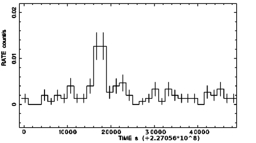
Figure 2: X-ray lightcurve for the ISO-Oph 85 source region ($20^{\prime\prime}$ radius, centered on the X-ray detection position) for the $50\,{\rm ks}$ of GTI of the observation $0305540701$ in which the flare is detected. Bin width $1500\,{\rm s}$. Bars represent $1\,{\rm\sigma}$ uncertainties.

To establish the duration of the flare exactly we run the XMM-Newton SAS edetect_chain source detection routine on the PN events that were filtered for different time slices ($10000\,{\rm s}$, $1000\,{\rm s}$, $500\,{\rm s,}$ and $100\,{\rm s}$) and in different energy bands ($0.3-2.0\,{\rm keV}$, $2.0-12.0\,{\rm keV}$, $0.3-12.0\,{\rm keV}$). We start with the longest interval ($10000\,{\rm s}$) and then proceed to successively shorter intervals when, in the longer one, a detection is present at a position consistent with that of the transient source. The transient duration is $\sim 2200\,{\rm s}$, during which the source is detected with a significance $>5\,{\rm\sigma}$ in the broad band $0.3-12.0\,{\rm keV}$. The distance between the X-ray source position and the HST/NICMOS position of ISO-Oph 85, which we will use as a reference position throughout this paper, is $2.2\,{\rm{}^{\prime\prime}}$. Following Severgnini et al. (2005), we extract the number of detected X-ray sources with USNO-B1 counterparts and calculate the probability of a random association between the detected transient and ISO-Oph 85 with $P=1-e^{-(\pi r^{2}\mu)}$, where $r$ is the X-ray source position uncertainty and $\mu\approx 10^{-4}{\rm src/arcsec^{2}}$, the numerical density of X-ray sources. The chance probability is $<0.6{\rm\%}$, suggesting that the identified transient X-ray source is associated with ISO-Oph 85.

The available XMM-Newton observations of the $\rho$ Ophiuchi core F are all DROXO observations (0305540501, 0305540601, 0305540701, 0305540901, 0305541001, and 0305541101) plus a previous $34\,{\rm ks}$-long observation 0111120201 (Vuong et al. 2003). Observation 0305541001 was excluded from spectral analysis because of the very high soft proton contamination. Adding up all the available observations, we have a grand total of $209.1\,{\rm ks}$ of observation (Good Time Intervals, GTI, free from soft proton background, obtained using the bkgoptrate SAS tool). We perform a search for other transients from ISO-Oph 85 with the automated pipeline and visually inspect the images but no other flares were detected. We perform an analysis of the X-ray emission, extracting the energy spectrum (for the flare) and the light curve (for the whole GTIs of the observation $0305540501$, in which the flare was detected, see Fig. 2).

In all DROXO observations the source position falls in a CCD gap for both MOS1 and MOS2 instruments, and so we only consider PN camera data. For each observation, the background is extracted for the flare analysis from a circular source-free region on the same CCD as the source. During the flare, we observe a net source count rate of $1.762\cdot 10^{-2}\pm 3.269\cdot 10^{-3}\,{\rm cts/s}$ in the band $0.3-12.0\,{\rm keV}$. An X-ray luminosity upper limit is obtained for the quiescent regime of the source outside the flare, in which the source is not detected in X-rays within $3{\rm\sigma}$ by edetect_chain. We consider all the GTIs of all the observations except the $2200\,{\rm s}$ of the flare as the quiescent time. For the quiescence, we obtain the background subtracted count rate upper limit at $3{\rm\sigma}$ from the formula for the signal-to-noise ratio

$$\frac{S}{N}=\frac{R_{src}\cdot T_{exp}}{\sqrt{R_{bkg}\cdot T_{exp}\cdot\frac{A_{src}}{A_{bkg}}+R_{src}\cdot T_{exp}}},$$ (1)

where the signal-to-noise ratio (S/N) is in $\sigma$ and set $(S/N)=3$, $R_{src}$ is the source count rate upper limit, $R_{bkg}$ is the background count rate, $T_{exp}$ is the total exposure time minus the flaring time ($206.9\,{\rm ks}$), and $A$ is the area of the extraction region. The background count rate is obtained from a background extraction region of area $\sim 7$ times the source region on the same CCD of the source extraction region. For the whole energy band ($0.3-12.0\,{\rm keV}$) we obtain a count rate upper limit of $4.91\cdot 10^{-4}\,{\rm cts/s}$.

4 X-ray properties of ISO-Oph 85

4.1 Flare light curve

The X-ray light curve (Fig. 2) shows a clear count excess in two $1500\,{\rm s}$-long adjacent time bins, corresponding to the detected flare. Because of the few counts ($39$ events from the whole $2200\,{\rm s}$ flaring time), it is not possible to infer the shape nor a decay time for the flare. We can only state that the decay time is less than $3000\,{\rm s}$ (twice the bin size). The low number of counts prohibits a standard spectral analysis. We observe a significant counts excess in the range $2.0-6.0\,{\rm keV}$ with respect to a pre-flare and post-flare $20\,{\rm ks}$ interval (including mainly background counts), which suggests an impulsive heating episode, as is typical for a flare.

4.2 Flare spectral analysis

A technique for performing a spectral analysis on few-counts spectra, using quantile quantities, was developed by Hong et al. (2004) and used for the analysis of YSOs spectral properties (e.g. Scelsi et al. 2007). We calculate the $25{\rm\%}$, $50{\rm\%,}$ and $75{\rm\%}$ quantiles of the counts of the flare observed from ISO-Oph 85. Then we derive the position of ISO-Oph 85 in the quantile space examined by Hong et al. (2004), defined by $Q_{25}/Q_{75}$ vs $Q_{50}/(1-Q_{50})$.

A $\log T$ vs $N_{\rm H}$ theoretical grid, predicted by an absorbed one-component coronal thermal model (WABS*APEC) with fixed abundance ($Z=0.3Z_{\odot}$ from Anders & Grevesse 1989), and modeled via $100000\,$s simulated spectra for a grid with $\log{T}$ from $6.50$ to $8.00$ and $N_{\rm H}$ from $1\cdotp 10^{20}\,{\rm cm^{-2}}$ to $N_{\rm H}=1\cdotp 10^{24}\,{\rm cm^{-2}}$, can be superimposed onto the phase space, thus giving the possibility to determine $kT$ and $N_{\rm H}$ values for each point in the quantile space (Fig.3). Following Scelsi et al. (2007), we compute this diagram for EPIC/PN data in the energy band $0.5-7.3\,{\rm keV}$. We extract a spectrum of the $2200\,{\rm s}$ total flare interval during which the source was detected, for a region with a radius of $20{\rm{}^{\prime\prime}}$ that is centered on the Hubble Space Telescope HST/NICMOS position of ISO-Oph 85, which has the highest precision. We extract a background spectrum from a region on the same detector CCD. From the position of ISO-Oph 85 on the quantile grid, we obtain $kT=1.15_{-0.65}^{+2.35}\,{\rm keV}$ and $N_{\rm H}=1.0_{-0.5}^{+1.2}\cdot 10^{23}\,{\rm cm^{-2}}$. The quantiles of ISO-Oph 85 represent the median value of the distribution that results when the quantile calculation is executed $1000$ times with randomly selected background photons according to the area-scaling factor between the source and background extraction regions. The error on the $x$ axis is derived from the statistical error of Hong et al. (2004). For each of the $1000$ quantile calculations, we have a statistical error. The distribution of these errors shows a peak at $0.075$. We take this value as our error. On the $y$ axis, this error is overestimated (see Hong et al. 2004). Thus, we do a simple error propagation on $Q_{25}/Q_{75}$ for each of the $1000$ calculations. The distribution of these errors shows a peak at $0.12$, which we assume to be our error on the $y$ axis.

To put the spectral properties of ISO-Oph 85 in context to those of the other YSOs in $\rho$ Oph, we calculate $Q_{25}/Q_{75}$ and $\log{(Q_{50}/(1-Q_{50}))}$ quantiles for all DROXO X-ray sources from Pillitteri et al. (2010) using the original extraction regions for source and background events of the full GTI filtered observing time. The background regions are larger than the source regions, typically by a factor of $\sim 3$. By way of an analogy to the case of ISO-Oph 85, and taking into account this scaling factor, we randomly select the appropriate fraction of photons from the background events files and perform the quantile determination for each DROXO source $1000$ times, each time with a different ensemble of background photons. The values shown in Fig. 3 represent the medians of the resulting distributions for $Q_{25}/Q_{75}$ and $\log(Q_{50}/(1-Q_{50}))$.

We classify the DROXO sources as Class I, flat, Class II, and Class III YSOs, according to their SED slope ($\alpha_{\rm SED}$) as defined and computed by Evans et al. (2009). Each YSO class is represented by a different plotting symbol in Fig. 3. Using the same definition of $\alpha_{\rm SED}$, in Sect. 5 we identify ISO-Oph 85 as a flat source. As can be seen from Fig. 3, the position of ISO-Oph 85 in the quantile phase space is consistent with that of Class I, “flat”, but also Class II sources in $\rho$ Oph, because of the large error bars. We note that the point of ISO-Oph 85 in the diagram is only due to the detected flare emission, while the DROXO stars are shown at their time-averaged spectral parameters.

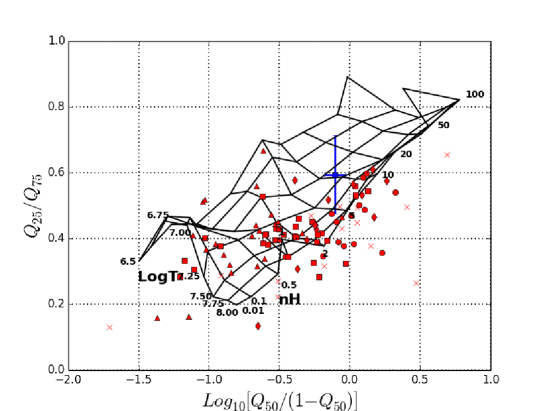
Figure 3: Phase space for the quantile analysis, with the parametric grid $\log T$, $N_{H}(10^{22}\,cm^{-2})$ superimposed. The flare on ISO-Oph 85 is represented by the blue square. DROXO time-averaged sources are represented by the following symbols: Class I (circles), Flat (diamonds), Class II (squares), Class III (triangles), undefined (x).

We then evaluate the X-ray flare emission properties with XSPEC . Within XSPEC we use a WABS $\cdot$ APEC model with an X-ray temperature of $kT=1.15\,{\rm keV}$ and a hydrogen column density $N_{H}=10^{23}\,{\rm cm^{-2}}$, as obtained from the quantile analysis, to get the $0.3-12\,{\rm keV}$ extinction-corrected X-ray flux during the flare ($f_{\rm x}=6.78\cdot 10^{-12}\,{\rm erg\,cm^{-2}\,{\rm s}^{-1}}$), the X-ray luminosity ($\log{L_{\rm x}\,[{\rm erg\,{\rm s}^{-1}}]}\,=31.6^{+2.0}_{-1.2}$) and the activity index ($\log{(L_{\rm x}/L_{\rm*,SB})}=-2^{+2}_{-1}$). The bolometric luminosity , $\log{L_{\rm*,SB}\,[{\rm erg\,{\rm s}^{-1}}]}=33.1^{+0.2}_{-0.1}$ is that obtained with the Stefan-Boltzmann law using the effective temperature and stellar radius of the best-fit model.

4.3 X-ray luminosity during quiescence

From the upper limit to the quiescent count rate (as given in Sect. 3) times a conversion factor, we obtain an X-ray flux and luminosity upper limit. We calculate the conversion factor from the flux obtained with XSPEC for a WABS$\cdot$ APEC model, using for $kT$ and $N_{H}$ the values from the quantile analysis. Given the distance of the source ($120\,pc$, Lombardi et al. 2008), we obtain the luminosity upper limit, that is $\log{L_{\rm x}}<29.5$. We note that the formally most conservative upper limit, which we can derive from the uncertainties of $N_{H}$ and $kT$ obtained from the quantile diagram, amounts to $\log{L_{\rm x}}<31.6$. By increasing the temperature, this luminosity decreases. Pillitteri et al. (2010) gives an upper limit of $\log{L_{\rm x}}<28.54$. This value was obtained with a different energy band ($0.3-10.0\,{\rm keV}$), model APEC component temperature ($kT=3.1\,{\rm keV}$), exposure time ($300.9\,{\rm ks}$), and a different absorption $N_{H}=2.3\cdot 10^{22}\,{\rm cm^{-2}}$. Moreover Pillitteri et al. (2010) calculate the upper limits using a different technique, following Damiani et al. (1997). This makes it difficult to compare the results. Nevertheless, $kT$ and $N_{H}$ calculated by Pillitteri et al. (2010) are consistent with the error bars of the ISO-Oph 85 point in Fig. 3.

5 Spectral energy distribution

The SED is key to understanding the evolutionary phase of a YSO. To this end, we collect all available photometric data for ISO-Oph85 from the literature and from data archives, we reanalyse Spitzer photometry, and we present as yet unpublished Herschel photometry of ISO-Oph85.

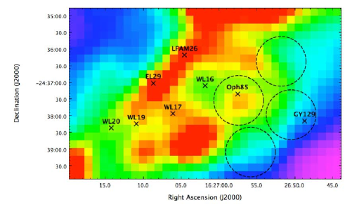
Figure 4: The Herschel/SPIRE $500\,{\rm\mu m}$ field with the position of ISO-Oph 85 and the other millimetric sources in the field of view (Motte et al. 1998). The source extraction region is shown, centered on the emission peak in SPIRE $500\,{\rm\mu m}$, together with the three circular regions used for the background evaluation, chosen to avoid contamination from other known bright YSOs and dust filaments.

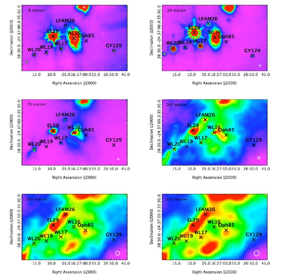
Figure 5: Images from Spitzer IRAC $8\,{\rm\mu m}$, MIPS $24\,{\rm\mu m}$, Herschel PACS $70\,{\rm\mu m}$, PACS $160\,{\rm\mu m,}$ and SPIRE $250\,{\rm\mu m}$ and $350\,{\rm\mu m}$ instruments with the HST/NICMOS position of ISO-Oph 85 and the position of the millimetric sources in the field of view (Motte et al. 1998). The instumental PSF is shown in the bottom right of each panel.

5.1 Multi-band photometry for ISO-Oph85

We cannot find any report of optical photometry for this object, presumably because of its large extinction. In some near-IR filters only the upper limits have been measured while mid-IR detections are available from various space missions (Spitzer, WISE, and ISOCAM). WISE data in the W3 and W4 bands are listed in Table 1 but are not considered further because they carry a source contamination flag and, in fact, no source is seen on the images of W3 and W4 bands. The photometric point with the longest wavelength is the $1.3\,{\rm mm}$ flux measured with the IRAM $30\,{\rm m}$ telescope by Motte et al. (1998).

The Spitzer data are taken from the Cores to Disks Legacy Project, (c2d, PI Evans, pid 177) We perform aperture photometry in the Spitzer IRAC bands ($3.6,4.5,5.6,$ and $8\,{\rm\mu m}$) by using the products available from the Spitzer Science Center (SSC) archive, and by adopting the recommended apertures at all wavelengths. These, for a reference pixel size of $1.2\,{\rm{}^{\prime\prime}}$, correspond to $12\,{\rm{}^{\prime\prime}}$ (source aperture) and to $14.4\,{\rm{}^{\prime\prime}}$ and $24\,{\rm{}^{\prime\prime}}$ (sky apertures). This way we obtain flux densities that agree within $5\,{\rm\%}$ with the values provided by the c2d collaboration (Evans et al. 2009). We also perform aperture photometry in the MIPS 24 ${\rm\mu m}$ band using a $13{\rm{}^{\prime\prime}}$ source aperture and $20{\rm{}^{\prime\prime}}$ to $32{\rm{}^{\prime\prime}}$ sky apertures. In this case, the computed flux is $\sim 40\,{\rm\%}$ higher than the value found by Evans et al. (2009). We investigate the source of a such a discrepancy. To this end, we notice that the c2d collaboration carried out their photometric measurements using a point-source profile-fitting approach. Along these lines, we perform PSF-fitting of our source in the Mopex/Apex environment, where, as an input PSF, we use the MIPS 24 $\mu m$ template that is publicly distributed by the SSC. After optimization of the Apex parameters, we obtain a flux-density value consistent with Evans et al. (2009), although with a poor reduced $\chi^{2}$ ($9.3$). Accordingly, and for consistency with the IRAC measurements, we decide to adopt the higher value derived from our aperture photometry. Spitzer MIPS $70\,{\rm\mu m}$ data also exist, but the quality of these data is typically rather poor compared to data at the same wavelength from Herschel PACS $70\,{\rm\mu m}$ since they, as we ascertain, show flux non-linearities and artifacts. This is the result of the different types of detectors. We thus decide not to use them.

We also analyse as yet unpublished submillimeter photometry from the Herschel mission (Fig. 4). For the position of ISO-Oph 85, archival Herschel PACS and SPIRE parallel mode observations at $70\,{\rm\mu m}$, $160\,{\rm\mu m}$, $250\,{\rm\mu m}$, $350\,{\rm\mu m}$, and $500\,{\rm\mu m}$ from the “Probing the origin of the initial mass function: A wide-field Herschel photometric survey of nearby star-forming cloud complexes.” program (KPGT_pandre_1) are available. The data have an angular resolution ranging from $6\,{\rm{}^{\prime\prime}}$ (at $70\,{\rm\mu m}$) to $35\,{\rm{}^{\prime\prime}}$ (at $500\,{\rm\mu m}$).

Given the difference in angular resolution between the NIR and mid-IR/submm data, it is important to make sure that the source that is visible in the lowest resolution band, i.e., Herschel/SPIRE $500\,{\rm\mu m}$, is indeed the same source that appears at shorter wavelengths. To this end, we adopt the location of the HST/NICMOS peak of emission as a reference. We then verify that the position of the peaks of emissions in each of the Herschel/PACS and SPIRE bands are within a FWHM from the position of the NICMOS peak, where the FWHM defines the PACS or SPIRE instrument resolution at a given wavelength. Fig. 4 shows an offset between the position of ISO-Oph 85 in HST/NICMOS and in Herschel SPIRE $500\,{\rm\mu m}$, but it is well within the angular resolution of SPIRE $500\,{\rm\mu m}$. Besides, there are no other millimetric sources that can be associated with the position of the emission peak in SPIRE $500\,{\rm\mu m}$, and generate confusion in the association with ISO-Oph 85. We, therefore, associate the SPIRE emission peak with ISO-Oph85, but caution that the positional offset between submm and IR is larger than for most other YSOs in the region.

We reduce Herschel data via the Herschel reduction pipeline. We perform aperture photometry in the PACS and SPIRE bands. At IR and submm wavelengths, the background emission surrounding ISO-Oph 85 is highly structured and position-dependent (see Fig. 5). For this reason, in each band we derive the source flux by taking the average of the values obtained by estimating the background from sky apertures that were placed at different locations in the source proximity. Using the median, the results do not change. Accordingly, the dispersion of the flux measurements around the mean value, combined with the intrinsic statistical errors, provide the flux errors. We use source and sky apertures of $12\,{\rm{}^{\prime\prime}}$, $22\,{\rm{}^{\prime\prime}}$, $40\,{\rm{}^{\prime\prime}}$ $50\,{\rm{}^{\prime\prime}}$, and $60{\rm{}^{\prime\prime}}$ at $70\,{\rm\mu m}$, $160\,{\rm\mu m}$, $250\,{\rm\mu m}$, $350\,{\rm\mu m}$, and $500\,{\rm\mu m}$. In the PACS bands, ISO-Oph 85 is barely visible above the background, therefore at $70\,{\rm\mu m}$ and $160\,{\rm\mu m}$ we are only able to place flux upper limits.

5.2 SED analysis

We model the SED of ISO-Oph 85 using the online SED fitter developed by Robitaille et al. (2007). This algorithm compares the observed photometric data set with a precomputed grid of $200000$ theoretical SEDs, which comprises $14$ free parameters that characterize the star, the disk, and the envelope of the hypothetical YSO. As pointed out by Robitaille et al. (2007), because of the complexity of the $\chi^{2}$ surface, this approach does not allow the true parameters of a YSO to be strictly determined, but, depending on the quality of the observed SED, it does allow meaningful constraints to be placed on a number of these parameters. Additional parameters are the interstellar extinction ($A_{\rm V}$) and the distance ($d$). Throughout the fitting process both $A_{\rm V}$ and $d$ are allowed to vary in a range that we set to $A_{\rm V}=0-80\,{\rm mag}$ and $d=120-130\,{\rm pc}$. These choices are motivated by the previous extinction estimate of Comeron et al. (1993) and the mean and spread of the distances cited in the literature for $\rho$ Oph (see Mamajek 2008, for a summary).

The filter list provided for Robitaille’s SED-fitting tool does not include the HST/NICMOS and the ISOCAM filters. Therefore, we have added these data points to the input of the SED fitter using the “monochromatic” option as an approximation. Given the uncertainties of the photometry related to zero-points and variability, the error introduced by neglecting the shape and width of the filter transmission is likely irrelevant. Following Robitaille et al. (2007), we impose a minimum of $10\,{\rm\%}$ flux error on all data points, and we base our assessment of the YSO parameters on the models with the smallest $\chi^{2}$ values, i.e., the $37$ models with $\chi^{2}-\chi^{2}_{\rm best}<3$ where $\chi^{2}_{\rm best}$ represents the best fit model ($20$ degrees of freedom). These are shown together with the observed SED in Fig. 6.

As can be seen in Fig. 6, a long-wavelength hump (representing emission from the envelope) is clearly visible. The hump is determined mainly by the Herschel data. If the hypothesis that the association with the Herschel peak is correct, this provides strong evidence for the protostellar nature of ISO-Oph 85. However, in this region of the SED the fit is not good. The uncertainties of the Herschel data are notoriously difficult to evaluate as a result of the strong spatial structure of the background emission at these wavelengths.

The most evident feature in the distribution of the bestfit parameters is related to the masses of the disk ($M_{d}$) and the envelope ($M_{\rm env}$). In Fig. 7 we compare the disk and envelope masses for the $37$ best-fit models to those of the $10000$ best fits. This shows that all best-fit models are among those from the available models with the highest envelope mass and accretion rate. The range of acceptable disk masses is large, while all bestfit models have high envelope mass. The range of best fit parameters is given in Table 2, where we also list the median and $25\,{\rm\%}$ and $75\,{\rm\%}$ quantiles for all fit parameters.

Figure 6: Spectral energy distribution of ISO-Oph 85 and of the $37$ best-model fits. Upper limits are represented as downward pointing triangles. The best-fit model is shown as solid black line and the other ‘statistically acceptable’ models as solid grey lines. The dashed line indicates the photospheric contribution of the best-fit model.

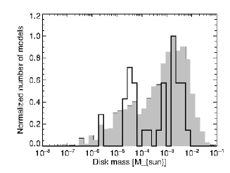
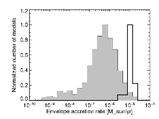
Figure 7: Distribution of model parameters for the $37$ best-fit models (black histograms) and for the $10000$ best-fitting models (grey histograms). The distributions are normalized to their peaks. From left to right: disk mass, envelope mass, envelope accretion rate.

Table 1: Photometry for ISO-Oph 85

Instrument	Filter	Mag	Emag	Flux	Error	Ref
				density
		[mag]	[mag]	[mJy]	[mJy]
HST/NICMOS3	$F110W$	21.5	—	0.004	—	(1)
2MASS	$J$	18.17	—	0.086	—	(2)
HST/NICMOS3	$F160W$	18.05	0.1	0.064	0.006	(1)
2MASS	$H$	16.74	—	0.210	—	(2)
2MASS	$K_{s}$	14.41	0.08	1.145	0.084	(2)
WISE	$W$1	11.98	0.02	4.94	0.09	(3)
Spitzer/IRAC	$I1$			7.5	0.75
Spitzer/IRAC	$I2$			10.3	1.03
WISE	$W2$	10.31	0.02	12.80	0.24	(3)
Spitzer/IRAC	$I3$			12.5	1.25
ISO/ISOCAM	$LW2$	9.37	0.1	15.00	4.00	(5)
Spitzer/IRAC	$I4$			11.8	3.2
WISE	$W3^{(c)}$	8.17	—	15.64	—	(3)
ISO/ISOCAM	$LW3$	8.10	0.10	11.00	7.00	(5)
WISE	$W4^{(c)}$	4.78	—	101.27	—	(3)
Spitzer/MIPS	$24\,\mu$m			118	77
Herschel/PACS	$70\,\mu$m			13320	—
Herschel/PACS	$160\,\mu$m			98890	—
Herschel/SPIRE	$250\,\mu$m			50610	14320
Herschel/SPIRE	$350\,\mu$m			24110	8939
Herschel/SPIRE	$500\,\mu$m			24110	3730
IRAM	$1.3mm$			70.00	15.0	(6)
(c) - confusion flag
(1) - (Allen et al. 2002), (2) - (Cutri et al. 2003), (3) - (Berriman 2008),
(4) - (Evans et al. 2009), (5) - (Bontemps et al. 2001),
(6) - (Andrews & Williams 2007).

Using the definitions of Robitaille et al. (2007), based on disk mass and envelope accretion rate, we can assign an evolutionary ‘stage’ to the best-fit models. Stage 0/I represents objects with significant infalling envelopes and possible disks, and Stage II denotes objects with optically thick disks and possible remains of an envelope. All best-fit models for the SED of ISO-Oph85 correspond to Stage 0/I, underpinning the early evolutionary stage of the object.

Table 2: SED best-fit parameters. Errors represent $25\%$ and $75\%$ quantiles for the 37 statistically acceptable models as defined in Sect. 5. ($A_{V,fit}$ - total extinction, $A_{V,cs}$ - circumstellar extinction, inside the envelope cavity)

Parameter	${\rm Allbestfit}$
$N_{\rm fit}$	$37$
$d[pc]$	$129.^{129.}_{123.}$
$A_{V,fit}[mag]$	$45.^{46.}_{42.}$
$A_{V,cs}[mag]$	$0.^{5.}_{0.}$
$M_{\rm d}*10^{3}[M_{\odot}]$	$0.81^{2.79}_{0.05}$
$\dot{M}_{\rm d}[M_{\odot}/yr]$	$-9.3^{-9.8}_{-8.6}$
$R_{\rm d,in}[AU]$	$6^{30}_{1}$
$R_{\rm d,out}[AU]$	$60^{493}_{42}$
$M_{\rm env}[M_{\odot}]$	$0.12^{0.17}_{0.09}$
$\dot{M}_{\rm env}[M_{\odot}/yr]$	$-4.91^{-4.76}_{-4.99}$
$R_{\rm env,in}[AU]$	$142^{784}_{42}$
$R_{\rm env,out}[AU]$	$1515^{1764}_{1395}$
$T_{\rm eff}[K]$	$2960^{2986}_{2851}$
$R_{\rm*}[R_{\odot}]$	$2.33^{2.56}_{2.18}$
$M_{\rm*}[M_{\odot}]$	$0.14^{0.15}_{0.12}$
$Age[Myr]$	$0.12^{0.15}_{0.09}$

In Sect.6 we compare ISO-Oph 85 to other X-ray sources in $\rho$ Oph for which we use the YSO classes given by Evans et al. (2009) that are based on the slope of their SEDs ($\alpha_{\rm SED}$) from $2-24\,{\rm\mu m}$. For ISO-Oph 85 Evans et al. (2009) determined $\alpha_{\rm SED}=-0.29$ using 2 MASS and Spitzer IRAC and MIPS 1 data. In our SED, we include analysis additional photometry from HST, WISE, and ISO. The SED slope we find from a least-squares fit to the data given in Table 1 in the $2-24\,{\rm\mu m}$ interval is $\alpha_{\rm SED}=0.10$. However, for consistency with the classification of the other DROXO sources, we also use the SED classification from Evans et al. (2009) for ISO-Oph 85. According to these results, ISO-Oph85 is considered a ‘flat spectrum’ source. We note, however, that the spectral index of ISO-Oph 85 is dominated by the low $K$-band flux and would be much steeper if the $K$-band were removed.

To summarize, our analysis of the SED of ISO-Oph85 establishes this object as a bona fide Class I protostar. The Herschel photometry gives credibility to this object being a Class I protostar. A slight doubt remains with this classification because of the offset between the optical/IR and submm position of the emission peaks. Given the large uncertainties in the Herschel fluxes, we do not lend too much weight to the values for the disk and envelope parameters derived from the SED fits. The stellar parameters are likely robust against the uncertainties in the submm fluxes but subject to uncertainties from the extinction.

6 Discussion and conclusions

The observation of a flare from ISO-Oph 85 is of twofold interest. Firstly, it provides a first validation of the discovery and science potential of the EXTraS project. Secondly, it gives insight into the physics, structure, and evolution of the YSOs. We showed that the analysis of the whole SED is fundamental for recognizing the evolutionary stage of YSOs, while the identification of the YSO class without submm data in the SED can lead to erroneous classification. This work also shows the possibility to perform a refined time-resolved analysis of the X-ray emission down to timescales that were previously inaccessible, and how such an analysis is fundamental for the understanding of the properties of the X-ray emission from YSOs. The object ISO-Oph 85 was detected in millimetric wavelength by Motte et al. (1998). Such long wavelength emissions can be a sign of protostellar nature, so the X-ray flaring activity from ISO-Oph 85 is particularly interesting, since X-ray flaring activity has rarely been observed in protostars. However, the wide gap in the SED between mid-IR (ISO/ISOCAM, Spitzer) data and the $1.3\,{\rm mm}$ detection leaves room for considering ISO-Oph 85 as a disk-bearing, envelope-free object, i.e., Class II source, as well. Our addition of Herschel submm photometry has been fundamental to removing this ambiguity. This makes the protostellar classification of ISO-Oph85 reliable, compared to other published X-ray detected objects with presumed Class I status, which have been classified using Spitzer data. As a note of caution, we point out that there is a small offset between the HST/NICMOS position of ISO-Oph 85 and the position of the emission peak in Herschel, even if it is clearly within the Herschel positional errors. Even if we consider this scenario as quite unlikely, we cannot exclude that the emission observed in Herschel might be associated with a starless core and not with ISO-Oph 85. In this case, the millimeter identification of ISO-Oph85 by Motte et al. (1998) would also likely be erroneous.

Another important aspect is that the X-ray emission from ISO-Oph85 was detected only as a result of our systematic time-resolved search for transient emission. Pillitteri et al. (2010) do not detect it in the same data set, based on time-averaged analysis, which highlights the discovery space inherent in time-resolved source detection.

We calculate rough estimates for $kT$ and $N_{H}$ from the analysis of energy quantiles: $kT=1.15_{-0.65}^{+2.35}\,{\rm keV}$ e $N_{H}=1.0_{-0.5}^{+1.2}\cdot 10^{23}\,{\rm cm^{-2}}$. At its lower end, the range of $N_{H}$ comprises the value we derive from the optical extinction $A_{V}=45^{+1}_{-3}$ that results from the SED fit. However, the gas-to-dust extinction law in star-forming regions is notoriously uncertain (Vuong et al. 2003). Using the above-mentioned spectral properties, we derive an X-ray luminosity of $\log{L_{X}}=31.1_{-1.2}^{+2.0}{\rm\,erg/s}$ for the flare of ISO-Oph85. The upper limit representing the quiescent stage of ISO-Oph 85 is $\log{L_{\rm X}}<29.5,$ as derived using the $N_{H}$ and $kT$ value measured in the quantile diagram. The spectral properties of the X-ray emitting plasma of ISO-Oph 85 are poorly constrained owing to low photon statistics. By making a comparison of the obtained temperature and absorption with other YSOs in DROXO, as detected by Pillitteri et al. (2010), we see that the flare emission from ISO-Oph 85 is located in the medium-temperature and high-absorption tail of the distribution. In particular, its position is closer to the clustering region of the Class I and flat spectrum sources than to the bulk of the Class II and Class III sources. We also note that Class I sources cluster near the boundary of our grid, at very high temperatures and high absorptions (see Fig. 3), and the same is true for ‘flat’ sources. Class II and especially Class III sources instead tend to cluster in the lower half of the grid, which corresponds with lower hydrogen column densities, and with a wide range of temperature. Comparing these results with the distribution of YSOs that were observed inside the Taurus Molecular Cloud by Scelsi et al. (2007), we note that the barycenter of their distribution is located at a lower value of hydrogen column density with respect to the barycenter of the distribution in the $\rho$ Ophiuchu cloud complex. This indicates a larger gas extinction in the $\rho$ Ophiuchi cloud, which is consistent with the larger dust extinction observed in the IR.

According to Grosso et al. (1997); Ozawa et al. (2005); Imanishi et al. (2001), and Flaccomio et al. (2003), the X-ray activity of a YSO roughly tends to increase as it gets older, moving from an earlier YSO class to a later one, meaning that Class 0 and I protostars have lower X-ray activity than T Tauri stars (Class II and Class III). Among Class I protostars, X-ray emission has only been detected for a few objects, while the X-ray emission of Class 0 objects has yet to be confirmed. The fraction of X-ray detection of Class I protostars is generally smaller than for Class II and III. It is not clear if this is due to the high absorption, as DROXO X-ray luminosity functions suggest, or because of intrinsically lower $L_{X}$. A third possibility for the low X-ray detection rate of Class I objects, suggested by our result for ISO-Oph85, is strong variability paired with low quiescent X-ray flux.

By adopting the submm peak as representative of the envelope of ISO-Oph85, the flare observed on ISO-Oph 85 confirms that protostars can exhibit strong X-ray activity. This behavior has already been noticed e.g., by Imanishi et al. (2001). However, most X-ray variability studies of protostars suffer from poor sensitivity and provide access only to coarse variability measures such as Kolmogorov-Smirnov (KS) statistics and poor time-sampling (Getman et al. 2007; Principe et al. 2014). The detection of a flare with $\sim 2$ decades amplitude is, therefore, notable. Since we observed only one flare in $209.1\,{\rm ks}$ of observation, we can state that X-ray flares of this amplitude or larger only occur in ISO-Oph 85 every $2.5\,{\rm d}$, roughly. This result is consistent with the flaring frequency observed in the Taurus Molecular Cloud (TMC) and in the Orion Nebula Cloud (ONC) by Stelzer et al. (2007). It is commonly thought that flares in embedded YSOs originate from coronal magnetic reconnection that is due to a stellar dynamo or to a magnetic reconnection between the field lines of the YSO itself, of the YSO and the disk, or of the disk itself. Since protostars are probably too young to have internal dynamo-like dynamics that are capable of producing intense magnetic reconnection from buoyant flux tubes (Hamaguchi et al. 2001) – as occurs in Sun-like stars – X-ray flares on protostars might be an indicator that the latter process dominates in X-ray emission. This could also mean that the stellar disk and possibly infalling envelopes have strong magnetic fields linked to that of the central forming protostar.

A systematic study of the X-ray flaring rate in $\rho$ Ophiuchi will be carried out in a separate paper, and will allow us to compare the flaring frequency in the $\rho$ Ophiuchi cloud complex with the results for TMC and ONC. A significant step forward in constraining the SED and understanding the YSO status could be made, for example, by using observations from the ALMA (Atacama Large Millimeter/submillimeter Array, Wootten & Thompson 2009).