On the Geometrization of Quantum Mechanics

Abstract

Nonrelativistic quantum mechanics is commonly formulated in terms of wavefunctions (probability amplitudes) obeying the static and the time-dependent Schrödinger equations (SE). Despite the success of this representation of the quantum world a wave-particle duality concept is required to reconcile the theory with observations (experimental measurements). A first solution to this dichotomy was introduced in the de Broglie-Bohm theory according to which a pilot wave (solution of the SE) is guiding the evolution of particle trajectories. Here, I propose a geometrization of quantum mechanics that describes the time evolution of particles as geodesic lines in a curved space, whose curvature is induced by the quantum potential. This formulation allows therefore the incorporation of all quantum effects into the geometry of space-time, as it is the case for gravitation in the general relativity.

I Introduction

Despite the enormous success of the theory of general relativity, not many attempts were made to apply the same geometrical approach to the description of the dynamics induced by other (fundamental) forces such as electrostatic in quantum mechanics Feynman et al. (2002). One of the main reasons for that, is the triumph of the wavefunction interpretation of the quantum world, and in particular of quantum electrodynamics and its description of the fundamental interactions as an exchange of virtual boson particles governed by the uncertainty principle. An important aspect that makes quantum mechanics hard to reconcile with a geometric description of the dynamics in terms of trajectories in configuration space is quantum correlation. In fact, wave mechanics as described by the Schrödinger equation (SE) offers a natural framework for the interpretation of coherence and decoherence effects and other peculiar properties of quantum mechanics like for instance the state superposition principle com (a). All these phenomena seem to rule out the possibility to include determinism in the description of quantum dynamics. Nonetheless, a first attempt in this direction was done by De Broglie and Bohm de Broglie (1926); Bohm (1952a, b); they introduced the concept of material point trajectories driven by a pilote wave that evolves according to the time-dependent Schrödinger equation for the system wave function $\psi(x_{1},\dots,x_{n},t)=\psi(\bm{x},t)$, with $x_{i}\in\mathbb{R}^{3}$. In this picture, Bohmian trajectories follow the flux lines of the quantum probability current, $\mathbf{j}(\bm{x})=(\mathbf{j}_{1}(\bm{x}),\dots,\mathbf{j}_{n}(\bm{x}))$ with $\mathbf{j}_{i}(\bm{x},t)=\hbar/m^{-1}\Im(\psi^{*}(\bm{x},t)\nabla_{i}\psi(\bm{x},t))$, which depends on the position of all particles in the system $(x_{1},\dots,x_{n})$ and introduces therefore nonlocality end (a) into the dynamics. Equivalently, the same dynamics can be reformulated in terms of configuration space trajectories following a Newton’s-like evolution (second order in time end (b) in which the quantum potential $Q(\bm{x},t)=-(\hbar^{2}/2m)\nabla^{2}A(\bm{x},t)/A(\bm{x},t)$ with $A(\bm{x},t)=(\psi^{*}(\bm{x},t)\psi(\bm{x},t))^{1/2}$ is added to the classical potential and contributes to the forces driving the system Holland (1993); Dürr et al. (1992). In the Bohmian mechanics Bohm (1952a) the time evolution of a quantum system is described by a single trajectory in phase space that is driven by the nonlocal quantum potential $Q(\bm{x},t)$, which is also a function of the entire configuration space and time.

In this work, I show that the effect of the Bohmian quantum potential can be absorbed into the geometry of the configuration space giving rise to a quantum dynamics described by deterministic trajectories evolving in a curved configuration space. The quantum potential is defined in the $3n$ dimensional configuration space, which makes this theory from-the-start a many-body formulation of the dynamics (for $n\geq 2$, where $n$ is the number of particles in the system of interest) and induces nonlocality in the dynamics associated to all constituent particles. The geometrization of the physical space is performed in a Finsler differential manifold Rund (1959), which is a nontrivial generalization of Riemann space in which the metric tensor depends from both positions and momenta. Different geometrization schemes based on a generalization of Riemann geometry were already proposed in the past, starting from the work of Weyl on electromagnetism Weyl (1918). Interesting extensions to quantum mechanics were more recently proposed by Novello and coworkers using a ‘Weyl integrable space’ (Q-wis) geometry Novello et al. (2011) obtained from a variational principle. In this work, we propose a geometrization scheme in which the metric tensor is derived from the quantum potential instead of being inferred; the price to pay is the extension from Riemann (and Q-wis geometry) to Finsler spaces. Finally, it is also interesting to mention the interesting approach by Ootsuka and Tanaka that deals with Feynman path-integrals in an extended configuration space endowed with a Finsler metric Ootsuka and E. (2010).

II Theory

II.1 Finsler geometry

For non-conservative systems described by time-dependent Lagrangians (and therefore time-dependent potentials like the quantum potential $Q(\bm{x},t)$), the dynamics can be reformulated by means of a homogeneous formalism in an extended configuration space of dimension ($3n+1$) where the additional variable corresponds to the time Schouten (1989); end (c). Defining $M$ the configuration space manifold and $TM$ the corresponding tangent space, if $\mathcal{L}:\mathbb{R}\times TM\rightarrow\mathbb{R}$ is the time-dependent Lagrangian function, then a corresponding generalized homogeneous Lagrangian $\Lambda:T(\mathbb{R}\times M)\rightarrow\mathbb{R}$ can be defined by

$$\Lambda(t,{\bm{x}},\dot{t},{\dot{\bm{x}}})\equiv\dot{t}\mathcal{L}(t,{\bm{x}},{\bm{x}}^{\prime})=\dot{t}\mathcal{L}(t,{\bm{x}},{\dot{\bm{x}}}/\dot{t})$$ (1)

with $(x_{i})^{\prime}=dx_{i}/dt$, $\dot{x}^{i}=dx_{i}/d\tau$, ($i=1,\dots,n$). In this formalism a new parameter $\tau(t)$ has been introduced to trace the progress of the system in the extended configuration spaces called the event space. As shown in Appendix A, the Euler-Lagrange equations corresponding to the Lagrangian $\Lambda(t,{\bm{x}},\dot{t},{\dot{\bm{x}}})$ are invariant with respect to any regular transformation of the parameter $\tau(t)$, and for the sub manifold obtained by setting $\dot{t}=1$ they reproduce the equations of motion for $\mathcal{L}(t,{\bm{x}},{\dot{\bm{x}}})$. In the extended configuration space, time is therefore risen to the rank of an additional generalized coordinate: $t=q_{0}\in\mathbb{R}$, and the dynamics is described in the $(3n+1)$-dimensional manifold (space of events) span by the generalised coordinates and velocities $\{\{q^{\alpha}\}_{\alpha=0}^{n},\{\dot{q}^{\alpha}\}_{\alpha=0}^{n}\}\equiv\{\bm{q},\dot{\bm{q}}\}$. In the following, I will relabel the coordinates of the canonical configuration space as $\{t,\{{x}_{i}\}_{i=1}^{n}\}$, and I will use $\{q^{\alpha}\}_{\alpha=0}^{n}$ for the extended configuration space according to the identification: $q^{0}=t$, $\dot{q}^{0}=dt/d\tau$, ${q}^{i}={x}_{i}$ ($i=1,\dots,n$) with $x_{i}\in\mathbb{R}^{3}$ and $q^{i}\in\mathbb{R}^{3}$; the velocities are defined as $\{\dot{q}^{\alpha}=dq_{\alpha}/d\tau\}_{\alpha=0}^{n}$, and $\{({x}_{i})^{\prime}=d{x}_{i}/dt\}_{i=1}^{n}$. For a Lagrangian with time-dependent potential $V({\bm{x}},t)$ of the form

$$\mathcal{L}(t,{\bm{x}},{\bm{x}}^{\prime})=T({\bm{x}}^{\prime})-V({\bm{x}},t)$$ (2)

we have therefore

$$\Lambda({\bm{q}},\dot{{\bm{q}}})=\mathcal{T}(\{\dot{q}^{i}\}^{n}_{i=1})/\dot{q}^{0}-V({\bm{q}})\,\dot{q}^{0}$$ (3)

with $T({\bm{x}}^{\prime})=\frac{1}{2}\sum_{i=1}^{n}m{(x_{i})^{\prime}}{(x_{i})^{\prime}}$ and $\mathcal{T}(\{\dot{q}^{i}\}^{n}_{i=1})=\frac{1}{2}\sum_{i=1}^{n}m(\dot{q}^{i})^{2}=T({\bm{x}}^{\prime})\,\,(\dot{q}^{0})^{2}$ .

In the case of conservative systems with time-independent potentials, using Jacobi’s theorem it is possible to describe a dynamics in a given potential with a geodesic motion in a Riemannian manifold with suited metric Abraham and Marsden (1994). In the non-conservative case, where the dynamics is described by a homogeneous Lagrangian $\Lambda({\bm{q}},\dot{{\bm{q}}})$ in Eq. (3), geometrization is obtained in the framework of Finsler’s spaces Rund (1959). In a Finsler space $M^{(3n+1)}$ with coordinates $\bm{q}=(q^{0},\dots,q^{n})$ the line element between two adjacent points in space is given by

$$ds=\left({g}_{\alpha\beta}(\bm{q},\dot{\bm{q}})dq^{\alpha}dq^{\beta}\right)^{1/2}=\Lambda(\bm{q},\dot{\bm{q}})d\tau\,.$$ (4)

(Einstein’s summation is assumed throughout the paper). The main difference with a Riemannian space is that the metric tensor ${g}_{\alpha\beta}(\bm{q},\dot{\bm{q}})$ depends also on velocities of the tangent space $TM^{(3n+1)}_{\bm{q}}$. The Finsler metric in Eq. (4) defines a dynamical system through the minimisation of the ‘action’ functional $I(\gamma)=\int_{\tau_{1}}^{\tau_{2}}\Lambda(\bm{q},\dot{\bm{q}})\,d\tau$ for a path $\gamma$ and given initial and final conditions ($\gamma(\tau_{1})$ and $\gamma(\tau_{2})$), when the following three conditions are fulfilled Caratheodory (1999) (i) positive homogeneity of degree one in the second argument, $\Lambda(\bm{q},k\dot{\bm{q}})=k\Lambda(\bm{q},\dot{\bm{q}}),k>0$, (ii) $\Lambda(\bm{q},\dot{\bm{q}})\neq 0,\forall\dot{\bm{q}}\neq 0$, and (iii) $\frac{\partial^{2}\Lambda^{2}(\bm{q},\dot{\bm{q}})}{\partial\dot{q}^{\alpha}\partial\dot{q}^{\beta}}\xi^{\alpha}\xi^{\beta}>0,\forall\bm{\xi}\neq\lambda\dot{\bm{q}}$.

The next step consists in the geometrization of the quantum dynamics using a Finsler’s metric derived from the time-dependent quantum Bohmian potential. This article is organised as following. First I derive a trajectory-based solution of the quantum dynamics starting from a general Lagrangian density for a complex scalar field $\phi(\bm{x},t)$. In a second step, I will introduce the geometrization of the resulting dynamics in a Finsler manifold Rund (1959) defined on the extended configuration space of dimension $(3n+1)$. The equations of motion are given by geodesic curves on a curved space-time manifold whose metric tensor is derived from the quantum potential, which in turn is a functional of the system wavefunction, $\phi(\bm{x},t)$.

II.2 Matter field and the trajectory representation of quantum dynamics.

Quantum dynamics can be formulated using from a canonical formalism in which the system wavefunction is treated as a classical complex scalar field $\phi(\bm{x},t)$ associated to the Lagrangian density Schleich et al. (2013); Takabayasi (1952) (using: $\{{q}^{i}\}^{n}_{i=1}=\{x_{i}\}_{i=1}^{n}\equiv\bm{x}$)

$$\mathscr{L}=\frac{i\hbar}{2}(\phi^{*}\dot{\phi}-\dot{\phi}^{*}\phi)-\frac{\hbar^{2}}{2m}\partial_{i}\phi\partial_{i}\phi^{*}-V\phi\phi^{*}\,.$$ (5)

Applying the principle of least-action to this Lagrangian density one obtained back the time dependent Schrödinger equation. The same formalism can also be generalised to the case of the Dirac equation Lurie (1968). Here we are interested in deriving a trajectory representation of the dynamics associated to the Lagrangian in Eq. 5. Following Takabayasi (1952); Holland (1993); Misner et al. (1973), we start from the field conservation law

$$\partial_{\alpha}\mathchoice{T_{\kern 0.0pt\hbox{$\scriptstyle\hbox{}\hbox{}\beta$}}^{\hbox{$\scriptstyle{}$}\kern 0.0pt\hbox{$\kern 0.0pt\scriptstyle\alpha\hbox{}$}}}{T_{\kern 0.0pt\hbox{$\scriptstyle\hbox{}\hbox{}\beta$}}^{\hbox{$\scriptstyle{}$}\kern 0.0pt\hbox{$\kern 0.0pt\scriptstyle\alpha\hbox{}$}}}{T_{\kern 0.0pt\hbox{$\scriptscriptstyle\hbox{}\hbox{}\beta$}}^{\hbox{$\scriptscriptstyle{}$}\kern 0.0pt\hbox{$\kern 0.0pt\scriptscriptstyle\alpha\hbox{}$}}}{T_{\kern 0.0pt\hbox{$\scriptscriptstyle\hbox{}\hbox{}\beta$}}^{\hbox{$\scriptscriptstyle{}$}\kern 0.0pt\hbox{$\kern 0.0pt\scriptscriptstyle\alpha\hbox{}$}}}=\frac{\partial\mathscr{L}}{\partial q_{\beta}}\,,$$ (6)

of the stress-energy-momentum tensor

$$\mathchoice{T_{\kern 0.0pt\hbox{$\scriptstyle\hbox{}\hbox{}\beta$}}^{\hbox{$\scriptstyle{}$}\kern 0.0pt\hbox{$\kern 0.0pt\scriptstyle\alpha\hbox{}$}}}{T_{\kern 0.0pt\hbox{$\scriptstyle\hbox{}\hbox{}\beta$}}^{\hbox{$\scriptstyle{}$}\kern 0.0pt\hbox{$\kern 0.0pt\scriptstyle\alpha\hbox{}$}}}{T_{\kern 0.0pt\hbox{$\scriptscriptstyle\hbox{}\hbox{}\beta$}}^{\hbox{$\scriptscriptstyle{}$}\kern 0.0pt\hbox{$\kern 0.0pt\scriptscriptstyle\alpha\hbox{}$}}}{T_{\kern 0.0pt\hbox{$\scriptscriptstyle\hbox{}\hbox{}\beta$}}^{\hbox{$\scriptscriptstyle{}$}\kern 0.0pt\hbox{$\kern 0.0pt\scriptscriptstyle\alpha\hbox{}$}}}=-\left[\frac{\partial\mathscr{L}}{\partial(\partial_{\alpha}\rho)}\partial_{\beta}\rho+\frac{\partial\mathscr{L}}{\partial(\partial_{\alpha}S)}\partial_{\beta}S\right]+\mathchoice{\delta_{\kern 0.0pt\hbox{$\scriptstyle\hbox{}\hbox{}\beta$}}^{\hbox{$\scriptstyle{}$}\kern 0.0pt\hbox{$\kern 0.0pt\scriptstyle\alpha\hbox{}$}}}{\delta_{\kern 0.0pt\hbox{$\scriptstyle\hbox{}\hbox{}\beta$}}^{\hbox{$\scriptstyle{}$}\kern 0.0pt\hbox{$\kern 0.0pt\scriptstyle\alpha\hbox{}$}}}{\delta_{\kern 0.0pt\hbox{$\scriptscriptstyle\hbox{}\hbox{}\beta$}}^{\hbox{$\scriptscriptstyle{}$}\kern 0.0pt\hbox{$\kern 0.0pt\scriptscriptstyle\alpha\hbox{}$}}}{\delta_{\kern 0.0pt\hbox{$\scriptscriptstyle\hbox{}\hbox{}\beta$}}^{\hbox{$\scriptscriptstyle{}$}\kern 0.0pt\hbox{$\kern 0.0pt\scriptscriptstyle\alpha\hbox{}$}}}\mathscr{L}\,,$$ (7)

where $S(\bm{x},t)/\hbar$ is the phase of $\phi(\bm{x},t)=A(\bm{x},t)e^{iS(\bm{x},t)/\hbar}$ and $\rho(\bm{x},t)=A^{2}(\bm{x},t)$. For the energy density, $\mathchoice{T_{\kern 0.0pt\hbox{$\scriptstyle\hbox{}\hbox{}0$}}^{\hbox{$\scriptstyle{}$}\kern 0.0pt\hbox{$\kern 0.0pt\scriptstyle 0\hbox{}$}}}{T_{\kern 0.0pt\hbox{$\scriptstyle\hbox{}\hbox{}0$}}^{\hbox{$\scriptstyle{}$}\kern 0.0pt\hbox{$\kern 0.0pt\scriptstyle 0\hbox{}$}}}{T_{\kern 0.0pt\hbox{$\scriptscriptstyle\hbox{}\hbox{}0$}}^{\hbox{$\scriptscriptstyle{}$}\kern 0.0pt\hbox{$\kern 0.0pt\scriptscriptstyle 0\hbox{}$}}}{T_{\kern 0.0pt\hbox{$\scriptscriptstyle\hbox{}\hbox{}0$}}^{\hbox{$\scriptscriptstyle{}$}\kern 0.0pt\hbox{$\kern 0.0pt\scriptscriptstyle 0\hbox{}$}}}$,

$$\frac{\partial\mathchoice{T_{\kern 0.0pt\hbox{$\scriptstyle\hbox{}\hbox{}0$}}^{\hbox{$\scriptstyle{}$}\kern 0.0pt\hbox{$\kern 0.0pt\scriptstyle 0\hbox{}$}}}{T_{\kern 0.0pt\hbox{$\scriptstyle\hbox{}\hbox{}0$}}^{\hbox{$\scriptstyle{}$}\kern 0.0pt\hbox{$\kern 0.0pt\scriptstyle 0\hbox{}$}}}{T_{\kern 0.0pt\hbox{$\scriptscriptstyle\hbox{}\hbox{}0$}}^{\hbox{$\scriptscriptstyle{}$}\kern 0.0pt\hbox{$\kern 0.0pt\scriptscriptstyle 0\hbox{}$}}}{T_{\kern 0.0pt\hbox{$\scriptscriptstyle\hbox{}\hbox{}0$}}^{\hbox{$\scriptscriptstyle{}$}\kern 0.0pt\hbox{$\kern 0.0pt\scriptscriptstyle 0\hbox{}$}}}(\bm{x},t)}{\partial t}+\mathchoice{T_{\kern 0.0pt\hbox{$\scriptstyle\hbox{}\hbox{}0,i$}}^{\hbox{$\scriptstyle{}$}\kern 0.0pt\hbox{$\kern 0.0pt\scriptstyle i\hbox{}$}}}{T_{\kern 0.0pt\hbox{$\scriptstyle\hbox{}\hbox{}0,i$}}^{\hbox{$\scriptstyle{}$}\kern 0.0pt\hbox{$\kern 0.0pt\scriptstyle i\hbox{}$}}}{T_{\kern 0.0pt\hbox{$\scriptscriptstyle\hbox{}\hbox{}0,i$}}^{\hbox{$\scriptscriptstyle{}$}\kern 0.0pt\hbox{$\kern 0.0pt\scriptscriptstyle i\hbox{}$}}}{T_{\kern 0.0pt\hbox{$\scriptscriptstyle\hbox{}\hbox{}0,i$}}^{\hbox{$\scriptscriptstyle{}$}\kern 0.0pt\hbox{$\kern 0.0pt\scriptscriptstyle i\hbox{}$}}}(\bm{x},t)=-\rho\frac{\partial V(\bm{x})}{\partial t}\,,$$ (8)

($\mathchoice{T_{\kern 0.0pt\hbox{$\scriptstyle\hbox{}\hbox{}0,i$}}^{\hbox{$\scriptstyle{}$}\kern 0.0pt\hbox{$\kern 0.0pt\scriptstyle i\hbox{}$}}}{T_{\kern 0.0pt\hbox{$\scriptstyle\hbox{}\hbox{}0,i$}}^{\hbox{$\scriptstyle{}$}\kern 0.0pt\hbox{$\kern 0.0pt\scriptstyle i\hbox{}$}}}{T_{\kern 0.0pt\hbox{$\scriptscriptstyle\hbox{}\hbox{}0,i$}}^{\hbox{$\scriptscriptstyle{}$}\kern 0.0pt\hbox{$\kern 0.0pt\scriptscriptstyle i\hbox{}$}}}{T_{\kern 0.0pt\hbox{$\scriptscriptstyle\hbox{}\hbox{}0,i$}}^{\hbox{$\scriptscriptstyle{}$}\kern 0.0pt\hbox{$\kern 0.0pt\scriptscriptstyle i\hbox{}$}}}=\partial\mathchoice{T_{\kern 0.0pt\hbox{$\scriptstyle\hbox{}\hbox{}0$}}^{\hbox{$\scriptstyle{}$}\kern 0.0pt\hbox{$\kern 0.0pt\scriptstyle i\hbox{}$}}}{T_{\kern 0.0pt\hbox{$\scriptstyle\hbox{}\hbox{}0$}}^{\hbox{$\scriptstyle{}$}\kern 0.0pt\hbox{$\kern 0.0pt\scriptstyle i\hbox{}$}}}{T_{\kern 0.0pt\hbox{$\scriptscriptstyle\hbox{}\hbox{}0$}}^{\hbox{$\scriptscriptstyle{}$}\kern 0.0pt\hbox{$\kern 0.0pt\scriptscriptstyle i\hbox{}$}}}{T_{\kern 0.0pt\hbox{$\scriptscriptstyle\hbox{}\hbox{}0$}}^{\hbox{$\scriptscriptstyle{}$}\kern 0.0pt\hbox{$\kern 0.0pt\scriptscriptstyle i\hbox{}$}}}/\partial x_{i}$) the conservation law can be reformulated in terms of the coupled differential equations for the amplitude and the phase of $\phi(\bm{x},t)$ (Appendix E)

$$\frac{\partial S(\bm{x},t)}{\partial t} =-\left(V(\bm{x})+Q(\bm{x},t)\right)-\frac{1}{2m}(\nabla S(\bm{x},t))^{2}\,$$ (9)

$$\frac{\partial A(\bm{x},t)}{\partial t} =-\frac{1}{2m}\big{(}2\nabla A(\bm{x},t)\nabla S(\bm{x},t)+A(\bm{x},t)\Delta S(\bm{x},t)\big{)}$$ (10)

where $Q(\bm{x},t)=-\frac{\hbar^{2}}{2m}\frac{\nabla^{2}A(\bm{x},t)}{A(\bm{x},t)}$ is the quantum potential. The dynamics described in Eq. (9) is equivalent to the Bohmian trajectory dynamics $\bm{x}^{\prime}(t)=v^{\phi}(\bm{x},t)$ for the vector field Bohm (1952b) (Appendix D)

$$v^{\phi}(\bm{x},t)=\frac{\hbar}{m}\Im\frac{\nabla_{\bm{x}}\phi(\bm{x},t)}{\phi(\bm{x},t)}\,.$$ (11)

Alternatively, one can identify Eq. (9) with the Hamilton-Jacobi equation for the ‘classical’ dynamics in the potential $V(\bm{x})+Q(\bm{x},t)$. Its solution by characteristics, for given initial conditions, corresponds to the trajectory solution of the Newton-like equation of motion Curchod and Tavernelli (2013); Curchod et al. (2013)

$$m\frac{d}{dt}\bm{x}^{\prime}(t)=-\nabla_{\bm{x}}(V(\bm{x})+Q(\bm{x},t))\,$$ (12)

with corresponding Lagrangian

$$\mathcal{L}(\bm{x},{\bm{x}}^{\prime},t)=\mathcal{T}(\bm{x}^{\prime})-(V(\bm{x})+Q(\bm{x},t)))\,.$$ (13)

In Eq. (12) $\bm{x}^{\prime}$ stands for $\partial\bm{x}/\partial t$ and $d/dt=\partial/\partial t+\bm{x}^{\prime}(t)\cdot\nabla$. However, a word of caution is recommended here, since the equivalence of the first- and second-order formulations of the dynamics (Eqs. (11) and  (12)) is still debated Valentini (1997).

The next step consists in the geometrization of the quantum dynamics obtained by absorbing the quantum potential $Q(\bm{x},t)$ into the metric tensor of the Finsler space. This is described in the following proposition.

II.3 Proposition

Consider a system of particles with coordinates $q^{i}\in\mathbb{R}^{3}$, $i=1,\dots,n$. The dynamics takes place in the extended configuration space with $q^{0}=t$, while the progress of the dynamics is measured in terms of a proper time parameter, $\tau$. For any given initial condition, the quantum dynamics associated to each configuration point follows a deterministic trajectory in the curved $3n+1$ dimensional space according to the geodesic equation ($\mu,\nu,\xi=0,\dots,3n$)

$$\ddot{q}^{\mu}+\mathchoice{\Gamma_{\kern 0.0pt\hbox{$\scriptstyle\hbox{}\hbox{}\nu\xi$}}^{\hbox{$\scriptstyle{}$}\kern 0.0pt\hbox{$\kern 0.0pt\scriptstyle\mu\hbox{}$}}}{\Gamma_{\kern 0.0pt\hbox{$\scriptstyle\hbox{}\hbox{}\nu\xi$}}^{\hbox{$\scriptstyle{}$}\kern 0.0pt\hbox{$\kern 0.0pt\scriptstyle\mu\hbox{}$}}}{\Gamma_{\kern 0.0pt\hbox{$\scriptscriptstyle\hbox{}\hbox{}\nu\xi$}}^{\hbox{$\scriptscriptstyle{}$}\kern 0.0pt\hbox{$\kern 0.0pt\scriptscriptstyle\mu\hbox{}$}}}{\Gamma_{\kern 0.0pt\hbox{$\scriptscriptstyle\hbox{}\hbox{}\nu\xi$}}^{\hbox{$\scriptscriptstyle{}$}\kern 0.0pt\hbox{$\kern 0.0pt\scriptscriptstyle\mu\hbox{}$}}}(\bm{q},\dot{\bm{q}})\dot{q}^{\nu}\dot{q}^{\xi}=-{g}^{\mu\nu}\partial V(\{q_{i}\}^{n}_{i=1})/\partial q^{\nu}$$ (14)

where $\mathchoice{\Gamma_{\kern 0.0pt\hbox{$\scriptstyle\hbox{}\hbox{}\nu\xi$}}^{\hbox{$\scriptstyle{}$}\kern 0.0pt\hbox{$\kern 0.0pt\scriptstyle\mu\hbox{}$}}}{\Gamma_{\kern 0.0pt\hbox{$\scriptstyle\hbox{}\hbox{}\nu\xi$}}^{\hbox{$\scriptstyle{}$}\kern 0.0pt\hbox{$\kern 0.0pt\scriptstyle\mu\hbox{}$}}}{\Gamma_{\kern 0.0pt\hbox{$\scriptscriptstyle\hbox{}\hbox{}\nu\xi$}}^{\hbox{$\scriptscriptstyle{}$}\kern 0.0pt\hbox{$\kern 0.0pt\scriptscriptstyle\mu\hbox{}$}}}{\Gamma_{\kern 0.0pt\hbox{$\scriptscriptstyle\hbox{}\hbox{}\nu\xi$}}^{\hbox{$\scriptscriptstyle{}$}\kern 0.0pt\hbox{$\kern 0.0pt\scriptscriptstyle\mu\hbox{}$}}}(\bm{q},\dot{\bm{q}})=\frac{1}{2}{g}^{\mu\sigma}({g}_{\sigma\xi,\nu}+{g}_{\sigma\nu,\xi}-{g}_{\nu\xi,\sigma})$ are the generalized connections (with ${g}_{\sigma\nu,\xi}=\partial_{{\xi}}{g}_{\sigma\mu}\equiv\partial g_{\sigma\mu}/\partial q_{\xi}$), and the space metric ${g}_{\mu\nu}$ is given by (Appendix C)

$$g_{\mu\nu}(\bm{q},\dot{\bm{q}})=\frac{1}{2}\frac{\partial^{2}\Lambda^{2}(\bm{q},\dot{\bm{q}})}{\partial\dot{q}^{\mu}\partial\dot{q}^{\nu}}\,$$ (15)

with

$$\Lambda(\bm{q},\dot{\bm{q}})=\mathcal{T}(\{\dot{q}^{i}\}^{n}_{i=1})/\dot{q}^{0}-Q(\bm{q})\dot{q}^{0}\,$$ (16)

and $\mathcal{T}(\{\dot{q}^{i}\}^{n}_{i=1})=(1/2)m(\dot{q}^{i})^{2}$ ($m$ is the particle mass). In Eqs. (14)-(16) we use $\tau=s$, where $s$ is the arclength defined by $ds=\Lambda(\bm{q},\dot{\bm{q}})d\tau$; $\bm{q}(t)$ and $\dot{\bm{q}}(t)$ are explicit functions of time, $V(\{{q}^{i}\}^{n}_{i=1})$ is the classical potential, and $Q(\{{q}^{i}\}^{n}_{i=1},t)=Q(\bm{x},t)$ is the quantum potential.

Proof: The proof is organised in two steps. (i) Starting from the Lagrangian density in Eq. (5) one can describe quantum dynamics using trajectories following the Newton-like equation of motion given in Eq. (12). Equivalently, the same result can be obtained following the derivation due to Bohm Bohm (1952a). (ii) The time-dependent Lagrangian associated to this dynamics (Eq. (16)), can be geometrized using Finsler’s approach outlined in Eqs. (2)-(4), which leads to the geodesic dynamics given in Eq. (14) (see also Appendices A and B). $\square$

In this proposition, a new description of quantum mechanics is proposed, in which the particle-wave duality is completely overcome. Matter is represented as point particles that move in a curved configuration space where the curvature is self-induced as well as generated, in a nonlocal fashion, by all other particles in the system; in other words, the metric tensor (and ultimately the curvature) depends on the coordinate of the particle of interest $q^{i}$, as well as from all other particles in the system, $q^{j}$, with $j\neq i$ com (b). The space curvature generated by the quantum potential evolves according to Eq. (9) and, therefore, the wave-like nature of quantum mechanics is confined to the geometric description of the space and voided from any mechanical property; all quantum effects are now absorbed into the metric of the configuration space com (c). It is worth mentioning that the geometrization of the configuration space is unique in the sense that is driven by the complex field $\phi(\bm{x},t)$, which is determined by the Lagrangian density Eq. (5) or, equivalently, the system of equations in (9) and  (10). The connection to the Schrödinger is discussed in the next section.

II.4 Relation to the Schrödinger dynamics

An ensemble of trajectories following the dynamics in Eq. (14) with properly chosen initial conditions describes the wavefunction dynamics of the time-dependent SE. In fact, when projected back to the $3n$ dimensional configuration space the trajectories defined in Eq. (14) reproduce exactly the Bohmian trajectories. This is evident from the correspondence of the characteristics associated to Eq. (9) with the Bohmian trajectories tangent to the vector field in Eq. (11). Therefore, when the initial configurations are sampled according to a given initial wavefunction density $|\phi(\bm{x},0)|^{2}$, the geodesics (or the corresponding Bohmian trajectories) evolve these points such that at a later time their density, $\rho(\bm{x},t)$, is consistent with the time-propagated wavefunction $\phi(\bm{x},t)$.

III Application

I illustrate the implications of the dynamics described in the Proposition by means of a simple example: the scattering of a Gaussian wavepacket with an Eckart-type potential barrier in one dimension (Fig. 1). This problem is described in details in Kendrick (2003). In this case, the Finsler’s space is described by an extended $2+2$ dimensional phase space with coordinates $\{q^{0}=t,\dot{q}^{0},q^{1},\dot{q}^{1}\}$, while the progress of the dynamics is measured by the parameter $\tau$. The wavepacket, $A(q^{1},0)=(2\beta/\pi)^{1/4}e^{-\beta(q^{1}-q_{c})^{2}}e^{ik(q^{1}-q_{c})}$ ($\beta=4$, $k=10.8842$) is initialised at position $q_{c}=2$, while the potential, $V(q^{1})=V_{0}\,\text{sech}^{2}(a(q^{1}-q_{p}))$, is fixed and centered at $q_{p}=7$. All quantities are given in atomic units (a.u.), $a=0.4$, $V_{0}=0.0365$. An ensemble of 200 trajectories is used to describe the wavepacket dynamics. They are initially distributed according the the probability $A^{2}(q^{1}(0))$, while $\dot{q}^{1}(0)=1$, $q^{0}(0)=0$ and $\dot{q}^{0}(0)=1$ for all trajectories. The time evolution of the wavepacket is depicted in Fig. 1 together with the corresponding snapshots of the quantum potential computed on the support of the wavepacket (inset of the upper panel), which is given by the values $q_{1}$ sampled by the 200 trajectories at a given value of $\tau$ (or time $t(\tau)$). The space curvature is defined as ($(\bm{q},\dot{\bm{q}})\equiv(q^{0}(t),\dot{q}^{0}(t),q^{1}(t),\dot{q}^{1}(t))$)

$$R(\bm{q},\dot{\bm{q}})=g^{\alpha\beta}(\bm{q},\dot{\bm{q}})R_{\alpha\beta}(\bm{q},\dot{\bm{q}})$$ (17)

where $R_{\alpha\beta}=\mathchoice{R_{\kern 0.0pt\hbox{$\scriptstyle\hbox{}\hbox{}\alpha\beta\gamma$}}^{\hbox{$\scriptstyle{}$}\kern 0.0pt\hbox{$\kern 0.0pt\scriptstyle\gamma\hbox{}$}}}{R_{\kern 0.0pt\hbox{$\scriptstyle\hbox{}\hbox{}\alpha\beta\gamma$}}^{\hbox{$\scriptstyle{}$}\kern 0.0pt\hbox{$\kern 0.0pt\scriptstyle\gamma\hbox{}$}}}{R_{\kern 0.0pt\hbox{$\scriptscriptstyle\hbox{}\hbox{}\alpha\beta\gamma$}}^{\hbox{$\scriptscriptstyle{}$}\kern 0.0pt\hbox{$\kern 0.0pt\scriptscriptstyle\gamma\hbox{}$}}}{R_{\kern 0.0pt\hbox{$\scriptscriptstyle\hbox{}\hbox{}\alpha\beta\gamma$}}^{\hbox{$\scriptscriptstyle{}$}\kern 0.0pt\hbox{$\kern 0.0pt\scriptscriptstyle\gamma\hbox{}$}}}$ is the Ricci tensor and

$$\mathchoice{R_{\kern 0.0pt\hbox{$\scriptstyle\hbox{}\hbox{}\alpha\beta\gamma$}}^{\hbox{$\scriptstyle{}$}\kern 0.0pt\hbox{$\kern 0.0pt\scriptstyle\gamma\hbox{}$}}}{R_{\kern 0.0pt\hbox{$\scriptstyle\hbox{}\hbox{}\alpha\beta\gamma$}}^{\hbox{$\scriptstyle{}$}\kern 0.0pt\hbox{$\kern 0.0pt\scriptstyle\gamma\hbox{}$}}}{R_{\kern 0.0pt\hbox{$\scriptscriptstyle\hbox{}\hbox{}\alpha\beta\gamma$}}^{\hbox{$\scriptscriptstyle{}$}\kern 0.0pt\hbox{$\kern 0.0pt\scriptscriptstyle\gamma\hbox{}$}}}{R_{\kern 0.0pt\hbox{$\scriptscriptstyle\hbox{}\hbox{}\alpha\beta\gamma$}}^{\hbox{$\scriptscriptstyle{}$}\kern 0.0pt\hbox{$\kern 0.0pt\scriptscriptstyle\gamma\hbox{}$}}} (\bm{q},\dot{\bm{q}})=\mathchoice{\Gamma_{\kern 0.0pt\hbox{$\scriptstyle\hbox{}\hbox{}\alpha\gamma,\beta$}}^{\hbox{$\scriptstyle{}$}\kern 0.0pt\hbox{$\kern 0.0pt\scriptstyle\delta\hbox{}$}}}{\Gamma_{\kern 0.0pt\hbox{$\scriptstyle\hbox{}\hbox{}\alpha\gamma,\beta$}}^{\hbox{$\scriptstyle{}$}\kern 0.0pt\hbox{$\kern 0.0pt\scriptstyle\delta\hbox{}$}}}{\Gamma_{\kern 0.0pt\hbox{$\scriptscriptstyle\hbox{}\hbox{}\alpha\gamma,\beta$}}^{\hbox{$\scriptscriptstyle{}$}\kern 0.0pt\hbox{$\kern 0.0pt\scriptscriptstyle\delta\hbox{}$}}}{\Gamma_{\kern 0.0pt\hbox{$\scriptscriptstyle\hbox{}\hbox{}\alpha\gamma,\beta$}}^{\hbox{$\scriptscriptstyle{}$}\kern 0.0pt\hbox{$\kern 0.0pt\scriptscriptstyle\delta\hbox{}$}}}(\bm{q},\dot{\bm{q}})-\mathchoice{\Gamma_{\kern 0.0pt\hbox{$\scriptstyle\hbox{}\hbox{}\alpha\beta,\gamma$}}^{\hbox{$\scriptstyle{}$}\kern 0.0pt\hbox{$\kern 0.0pt\scriptstyle\delta\hbox{}$}}}{\Gamma_{\kern 0.0pt\hbox{$\scriptstyle\hbox{}\hbox{}\alpha\beta,\gamma$}}^{\hbox{$\scriptstyle{}$}\kern 0.0pt\hbox{$\kern 0.0pt\scriptstyle\delta\hbox{}$}}}{\Gamma_{\kern 0.0pt\hbox{$\scriptscriptstyle\hbox{}\hbox{}\alpha\beta,\gamma$}}^{\hbox{$\scriptscriptstyle{}$}\kern 0.0pt\hbox{$\kern 0.0pt\scriptscriptstyle\delta\hbox{}$}}}{\Gamma_{\kern 0.0pt\hbox{$\scriptscriptstyle\hbox{}\hbox{}\alpha\beta,\gamma$}}^{\hbox{$\scriptscriptstyle{}$}\kern 0.0pt\hbox{$\kern 0.0pt\scriptscriptstyle\delta\hbox{}$}}}(\bm{q},\dot{\bm{q}})+$$

$$\mathchoice{\Gamma_{\kern 0.0pt\hbox{$\scriptstyle\hbox{}\hbox{}\alpha\gamma$}}^{\hbox{$\scriptstyle{}$}\kern 0.0pt\hbox{$\kern 0.0pt\scriptstyle\lambda\hbox{}$}}}{\Gamma_{\kern 0.0pt\hbox{$\scriptstyle\hbox{}\hbox{}\alpha\gamma$}}^{\hbox{$\scriptstyle{}$}\kern 0.0pt\hbox{$\kern 0.0pt\scriptstyle\lambda\hbox{}$}}}{\Gamma_{\kern 0.0pt\hbox{$\scriptscriptstyle\hbox{}\hbox{}\alpha\gamma$}}^{\hbox{$\scriptscriptstyle{}$}\kern 0.0pt\hbox{$\kern 0.0pt\scriptscriptstyle\lambda\hbox{}$}}}{\Gamma_{\kern 0.0pt\hbox{$\scriptscriptstyle\hbox{}\hbox{}\alpha\gamma$}}^{\hbox{$\scriptscriptstyle{}$}\kern 0.0pt\hbox{$\kern 0.0pt\scriptscriptstyle\lambda\hbox{}$}}}(\bm{q},\dot{\bm{q}})\mathchoice{\Gamma_{\kern 0.0pt\hbox{$\scriptstyle\hbox{}\hbox{}\lambda\beta$}}^{\hbox{$\scriptstyle{}$}\kern 0.0pt\hbox{$\kern 0.0pt\scriptstyle\delta\hbox{}$}}}{\Gamma_{\kern 0.0pt\hbox{$\scriptstyle\hbox{}\hbox{}\lambda\beta$}}^{\hbox{$\scriptstyle{}$}\kern 0.0pt\hbox{$\kern 0.0pt\scriptstyle\delta\hbox{}$}}}{\Gamma_{\kern 0.0pt\hbox{$\scriptscriptstyle\hbox{}\hbox{}\lambda\beta$}}^{\hbox{$\scriptscriptstyle{}$}\kern 0.0pt\hbox{$\kern 0.0pt\scriptscriptstyle\delta\hbox{}$}}}{\Gamma_{\kern 0.0pt\hbox{$\scriptscriptstyle\hbox{}\hbox{}\lambda\beta$}}^{\hbox{$\scriptscriptstyle{}$}\kern 0.0pt\hbox{$\kern 0.0pt\scriptscriptstyle\delta\hbox{}$}}}(\bm{q},\dot{\bm{q}})-\mathchoice{\Gamma_{\kern 0.0pt\hbox{$\scriptstyle\hbox{}\hbox{}\alpha\beta$}}^{\hbox{$\scriptstyle{}$}\kern 0.0pt\hbox{$\kern 0.0pt\scriptstyle\lambda\hbox{}$}}}{\Gamma_{\kern 0.0pt\hbox{$\scriptstyle\hbox{}\hbox{}\alpha\beta$}}^{\hbox{$\scriptstyle{}$}\kern 0.0pt\hbox{$\kern 0.0pt\scriptstyle\lambda\hbox{}$}}}{\Gamma_{\kern 0.0pt\hbox{$\scriptscriptstyle\hbox{}\hbox{}\alpha\beta$}}^{\hbox{$\scriptscriptstyle{}$}\kern 0.0pt\hbox{$\kern 0.0pt\scriptscriptstyle\lambda\hbox{}$}}}{\Gamma_{\kern 0.0pt\hbox{$\scriptscriptstyle\hbox{}\hbox{}\alpha\beta$}}^{\hbox{$\scriptscriptstyle{}$}\kern 0.0pt\hbox{$\kern 0.0pt\scriptscriptstyle\lambda\hbox{}$}}}(\bm{q},\dot{\bm{q}})\mathchoice{\Gamma_{\kern 0.0pt\hbox{$\scriptstyle\hbox{}\hbox{}\lambda\gamma$}}^{\hbox{$\scriptstyle{}$}\kern 0.0pt\hbox{$\kern 0.0pt\scriptstyle\delta\hbox{}$}}}{\Gamma_{\kern 0.0pt\hbox{$\scriptstyle\hbox{}\hbox{}\lambda\gamma$}}^{\hbox{$\scriptstyle{}$}\kern 0.0pt\hbox{$\kern 0.0pt\scriptstyle\delta\hbox{}$}}}{\Gamma_{\kern 0.0pt\hbox{$\scriptscriptstyle\hbox{}\hbox{}\lambda\gamma$}}^{\hbox{$\scriptscriptstyle{}$}\kern 0.0pt\hbox{$\kern 0.0pt\scriptscriptstyle\delta\hbox{}$}}}{\Gamma_{\kern 0.0pt\hbox{$\scriptscriptstyle\hbox{}\hbox{}\lambda\gamma$}}^{\hbox{$\scriptscriptstyle{}$}\kern 0.0pt\hbox{$\kern 0.0pt\scriptscriptstyle\delta\hbox{}$}}}(\bm{q},\dot{\bm{q}})$$ (18)

is the Riemann curvature tensor with $\mathchoice{\Gamma_{\kern 0.0pt\hbox{$\scriptstyle\hbox{}\hbox{}\alpha\gamma,\beta$}}^{\hbox{$\scriptstyle{}$}\kern 0.0pt\hbox{$\kern 0.0pt\scriptstyle\delta\hbox{}$}}}{\Gamma_{\kern 0.0pt\hbox{$\scriptstyle\hbox{}\hbox{}\alpha\gamma,\beta$}}^{\hbox{$\scriptstyle{}$}\kern 0.0pt\hbox{$\kern 0.0pt\scriptstyle\delta\hbox{}$}}}{\Gamma_{\kern 0.0pt\hbox{$\scriptscriptstyle\hbox{}\hbox{}\alpha\gamma,\beta$}}^{\hbox{$\scriptscriptstyle{}$}\kern 0.0pt\hbox{$\kern 0.0pt\scriptscriptstyle\delta\hbox{}$}}}{\Gamma_{\kern 0.0pt\hbox{$\scriptscriptstyle\hbox{}\hbox{}\alpha\gamma,\beta$}}^{\hbox{$\scriptscriptstyle{}$}\kern 0.0pt\hbox{$\kern 0.0pt\scriptscriptstyle\delta\hbox{}$}}}=\partial\mathchoice{\Gamma_{\kern 0.0pt\hbox{$\scriptstyle\hbox{}\hbox{}\alpha\gamma$}}^{\hbox{$\scriptstyle{}$}\kern 0.0pt\hbox{$\kern 0.0pt\scriptstyle\delta\hbox{}$}}}{\Gamma_{\kern 0.0pt\hbox{$\scriptstyle\hbox{}\hbox{}\alpha\gamma$}}^{\hbox{$\scriptstyle{}$}\kern 0.0pt\hbox{$\kern 0.0pt\scriptstyle\delta\hbox{}$}}}{\Gamma_{\kern 0.0pt\hbox{$\scriptscriptstyle\hbox{}\hbox{}\alpha\gamma$}}^{\hbox{$\scriptscriptstyle{}$}\kern 0.0pt\hbox{$\kern 0.0pt\scriptscriptstyle\delta\hbox{}$}}}{\Gamma_{\kern 0.0pt\hbox{$\scriptscriptstyle\hbox{}\hbox{}\alpha\gamma$}}^{\hbox{$\scriptscriptstyle{}$}\kern 0.0pt\hbox{$\kern 0.0pt\scriptscriptstyle\delta\hbox{}$}}}/\partial q^{\beta}$. The lower panel of Fig. 1 shows the value of the curvature, $R(q_{(i)}^{1}(\tau_{j});q_{(i)}^{0}(\tau_{j}),\dot{q}_{(i)}^{0}(\tau_{j}),\dot{q}_{(i)}^{1}(\tau_{j}))$, on the support of the wavepacket, sampled by the trajectories labeled with $i$ ($i=1,\dots,200$), at different values of $t$ ranging from $t=50$ to $t=2100$ in intervals of $100$. Initially ($t<400$), the curvature is positive for all points (dark brown lines), while at later times we observe regions of positive and negative curvature. Towards the end of the simulation the curvature become strongly negative for all points at the right-hand side of the potential barrier.

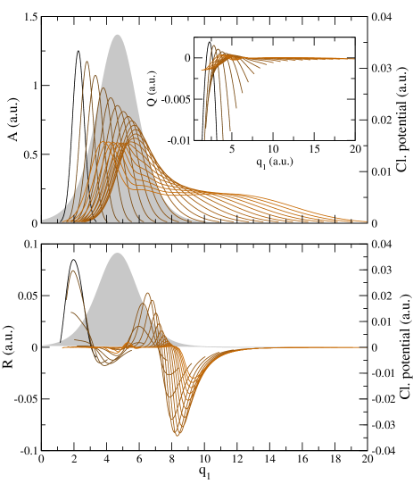
Figure 1: Upper panel: Time evolution of the nuclear wavepacket. Snapshots are taken between time $t=50$ (dark brown) and $t=2100$ (light brown) in intervals of $100$. The inset shows the dynamics of the quantum potential in the same time interval. Lower panel: Time evolution of the space curvature $R(\bm{q},\dot{\bm{q}})$ projected along the space coordinate $q_{1}$ (same color code as for the upper panel). The static classical potential (Eckart barrier) is shown in gray. All quantities are measured in atomic units.

This becomes more evident if we observe the dynamics in the plane defined by the coordinates $q^{1}$ and $\dot{q}^{1}$. Fig. 2 shows the time evolution of the system as a series of line fronts in the $q^{1}$, $\dot{q}^{1}$ plane; each line is defined by the points $\{q^{1}_{(i)},\dot{q}^{1}_{(i)}\}$ at a given time $t$, where the index $i$ runs over the ensemble of trajectories. The dynamics of two representative trajectories projected on the same plane (black lines) shows a first ‘convergent’ behavior (signature of a positive curvature) followed by a diverging behavior (negative curvature). Of particular interest is the analysis of the time dilation effect. The right inset in Fig. 2 shows the line fronts in the $(q^{1},q^{0})$ plane, each line corresponding to a fixed value of the ‘reference time’ $\tau$. We observe that the local time, $q^{0}(\tau)$, runs faster for the points on the right-hand side of the wavepacket (larger gaps between the line) than for the points on the left-hand side that are recoiled by the potential.

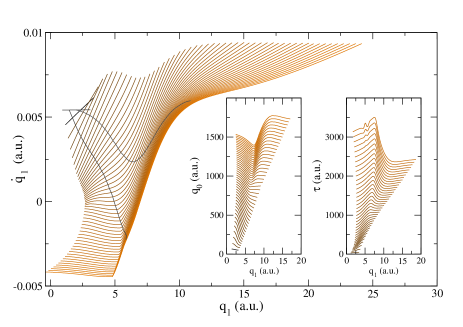
Figure 2: Time evolution of the line fronts defined by the variables $\{q_{(i)}^{1}(t),\dot{q}_{(i)}^{1}(t)\}$ along the trajectories, $i=1,\dots,200$ at regular time intervals of $50$ a.u. starting from $t=0$. Color code: brown scale from black (t=0 a.u.) to orange (t=2100 a.u.). Two trajectories are shown in black. The same dynamics projected on the $\{q^{1},q^{0}\}$ and $\{q^{1},\tau\}$ planes is shown in the two insets.

IV Conclusions

In conclusion, in this article I present a geometrization of quantum dynamics according to which all non-classical quantum effects are included in the geometry of an extended phase space (that includes time) of dimension $6n+2$. The particles evolve along geodesic lines in a curved Finsler manifold modeled by the quantum potential. In this framework, the particle-wave duality of conventional quantum mechanics is replaced by deterministic particle dynamics evolving on a curved manifold, where the curvature is derived from the nonlocal quantum potential that depends on the position of all particles in the system (independently from their reciprocal distance and interaction). This picture of quantum dynamics is well suited for the understanding of nonlocality in quantum mechanics including, for instance, the self-interference of single particles (electrons or molecules) on a double slit Nairz et al. (2001); Juffmann et al. (2009, 2012), and the interpretation of the Mach-Zehnder’s interferometer Philippidis et al. (1979); Rarity et al. (1990), for which particle-wave duality is required according to the classical interpretation of quantum mechanics. In the first situation, the interference pattern results from the nonlocality of the quantum potential, $Q({\bm{q}}_{\text{slit}},\bm{q}_{\text{mol}},t)$, which entangles the single particle dynamics, $\bm{q}_{\text{mol}}(t)$, with the one of the device (double slit). Mach-Zehnder’s interference at a distance is made possible by the fact that quantum information is not just carried by the particle dynamics but also includes a component from the propagation of the configuration space curvature end (d); com (d). This interpretation of quantum dynamics offers in addition a very simple solution to the measurement problem in quantum mechanics; in fact, like in Bohmian mechanics Bohm (1952a), the trajectories describe deterministic paths in space and the transition to the classical world does not require the concept of wavefunction collapse. The wavefunction character of the quantum state and its dynamics is now confined to the characterization of the curvature of the configuration space of each constituent particle, while the system evolves along deterministic geodesic curves. Finally, the geometrization of quantum mechanics offers a clear opportunity for the unification with Einstein’s theory of general relativity.

Appendix A Equivalence of the dynamics described by $\Lambda(\bm{q},\dot{\bm{q}})$ and by $\mathcal{L}(\bm{x},\dot{\bm{x}},t)$

The demonstration of the equivalence of the dynamics generated by $\Lambda(\{q^{\alpha}\}_{\alpha=0}^{n},\{\dot{q}^{\alpha}\}_{\alpha=0}^{n})=\Lambda(\bm{q},\dot{\bm{q}})$ and $\mathcal{L}(t,\{x_{i}\}_{i=1}^{n},\{({x}_{i})^{\prime}\}_{i=1}^{n})$ is given in two parts. I will use the following notation: $q^{0}=t$, $\dot{q}^{0}=dt/d\tau$, ${q}^{i}={x}_{i}$ ($i=1,\dots,n$) with $x_{i}\in\mathbb{R}^{3}$ and $q^{i}\in\mathbb{R}^{3}$; the velocities are defined as $\{\dot{q}^{\alpha}=dq^{\alpha}/d\tau\}_{\alpha=0}^{n}$, and $\{x^{\prime}_{i}=d{x}_{i}/dt\}_{i=1}^{n}$. In the first part, I show that the Lagrange dynamics in the extended ($3n+1$) configuration space (governed by the Lagrangian $\Lambda(\{q^{\alpha}\}^{n}_{\alpha=0},\{\dot{q}^{\alpha}\}^{n}_{\alpha=0}$) is equivalent to the standard Lagrange formulation of dynamics in the $n$-dimensional configuration space (governed by the Lagrangian $\mathcal{L}(t,\{q^{i}\}^{n}_{i=1},\{\dot{q}^{i}\}^{n}_{i=1})$. The dependence on $\{q^{\alpha}\}^{n}_{\alpha=0}$ and $\{q^{i}\}^{n}_{i=1}$ indicates a dependence of the full ($3n+1$) and ($3n$) dimensional manifolds, respectively. In the following I will drop the indexes when referring to the entire vectors and use them only for the components:

$$\{x_{i}\}_{i=1}^{n}=\{q^{i}\}_{i=1}^{n}\equiv\bm{x},\,\{(x_{i})^{\prime}\}_{i=1}^{n}\equiv\bm{x}^{\prime},\,\{q^{\alpha}\}_{\alpha=0}^{n}\equiv\bm{q},\,\text{and}\,\{\dot{q}^{\alpha}\}_{\alpha=0}^{n}\equiv\bm{\dot{}}{\bm{q}}\,.$$ (A.1)

In the second step, I show that the Lagrange dynamics in the extended ($3n+1$) configuration space can be formulated as a geodesic motion in a curved manifold.

The addition of a classical time-independent potential $V(\bm{x})$ will also be considered at the end of this section.

Step 1.

The Lagrange system obtained from the minimisation of the of the action functional $I(\gamma)=\int_{\tau_{1}}^{\tau_{2}}\Lambda(\bm{q},\dot{\bm{q}})\,d\tau$,

$$\frac{d}{d\tau}\left(\frac{\partial\Lambda(\bm{q},\dot{\bm{q}})}{\partial\dot{q}^{\alpha}}\right)-\frac{\partial\Lambda(\bm{q},\dot{\bm{q}})}{\partial{q}^{\alpha}}=0\,,\quad\quad(\alpha=0,\dots,n)$$ (A.2)

consists of $3n+1$ equations among which only $3n$ are independent and correspond to the equations of motion associated to $\mathcal{L}(\bm{q},\dot{\bm{q}})$. To show the linear dependence of the $3n+1$ Lagrange equations, we first make use of the homogeneity condition of degree one in the velocity ($\Lambda(\bm{q},k\dot{\bm{q}})=k\Lambda(\bm{q},\dot{\bm{q}}),k>0$), which according to Euler’s theorem gives (H. Rund, Ref. Rund (1959), pp. 3-4)

$$\frac{\partial\Lambda(\bm{q},\dot{\bm{q}})}{\partial\dot{q}^{\alpha}}\dot{q}^{\alpha} =\Lambda(\bm{q},\dot{\bm{q}})$$ (A.3)

$$\frac{\partial^{2}\Lambda(\bm{q},\dot{\bm{q}})}{\partial\dot{q}^{\alpha}\partial\dot{q}^{\beta}}\dot{q}^{\alpha} =0\,,$$ (A.4)

with (see definitions in the main text)

$$\Lambda(\bm{q},\dot{\bm{q}})=\mathcal{T}(\dot{\bm{q}})/\dot{q}^{0}-Q(\bm{x},t)\dot{q}^{0}\,.$$ (A.5)

The following relation can therefore be established

$$\sum_{\alpha}\dot{q}^{\alpha}\left(\frac{d}{d\tau}\left(\frac{\partial\Lambda(\bm{q},\dot{\bm{q}})}{\partial\dot{q}^{\alpha}}\right)-\frac{\partial\Lambda(\bm{q},\dot{\bm{q}})}{\partial{q}^{\alpha}}\right) =\frac{d}{d\tau}\sum_{\alpha}\left(\dot{q}^{\alpha}\frac{\partial\Lambda(\bm{q},\dot{\bm{q}})}{\partial{q}^{\alpha}}\right)-\sum_{\alpha}\left(\ddot{q}^{\alpha}\frac{\partial\Lambda(\bm{q},\dot{\bm{q}})}{\partial\dot{q}^{\alpha}}+\dot{q}^{\alpha}\frac{\partial\Lambda(\bm{q},\dot{\bm{q}})}{\partial{q}^{\alpha}}\right)$$

$$=\frac{d}{d\tau}\Lambda(\bm{q},\dot{\bm{q}})-\frac{d}{d\tau}\Lambda(\bm{q},\dot{\bm{q}})=0\,.$$ (A.6)

The system in Eq. (A.2) is therefore equivalent to the $3n$ standard Lagrange equations

$$\frac{d}{dt}\left(\frac{\partial\mathcal{L}(t,\bm{x},{\bm{x}}^{\prime})}{\partial x^{\prime}_{i}}\right)-\frac{\partial\mathcal{L}(t,\bm{x},{\bm{x}}^{\prime})}{\partial{x}_{i}}=0\,,\quad\quad(i=1,\dots,n)\,.$$ (A.7)

while the extra equation sets the freedom for the choice of $\tau(q_{0})$. To show this, we take the choice $\tau=t$ and therefore $\dot{q}^{0}=1$. Substituting

$$\Lambda(\bm{q},\dot{\bm{q}})=\left(T(\bm{x}^{\prime})-Q(\{q_{i}\}_{i=1}^{n},t)\right)\,\dot{q}^{0}=\mathcal{L}(t,\bm{x},{\bm{x}}^{\prime})$$ (A.8)

into Eq. (A.2) we obtained exactly Eq. (A.7) (for $i=1,\dots,n$).

Step 2.

The demonstration of the correspondence between the Euler-Lagrange equations for $\Lambda(\bm{q},\dot{\bm{q}})$ and the geodesic equation in the curved manifold characterised by the metric tensor $g_{\alpha\beta}(\bm{q},\dot{\bm{q}})=\frac{1}{2}\frac{\partial^{2}\Lambda^{2}(\bm{q},\dot{\bm{q}})}{\partial\dot{q}^{\alpha}\partial\dot{q}^{\beta}}$ follows closely the one given by H. Rund (Ref. Rund (1959), Chapter II, paragraph 2).

Starting from the Euler-Lagrange equations formulated in the arc-length parameter $s$ (for which $\Lambda(\bm{q},\dot{\bm{q}})=1$ along the path) ,

$$\frac{d}{ds}\left(\frac{\partial\Lambda(\bm{q},\dot{\bm{q}})}{\partial\dot{q}^{\alpha}}\right)-\frac{\partial\Lambda(\bm{q},\dot{\bm{q}})}{\partial q^{\alpha}}=0\,,\quad(\alpha=0,\dots n)$$ (A.9)

with the definition

$$g_{\alpha\beta}(\bm{q},\dot{\bm{q}})=\frac{1}{2}\frac{\partial^{2}\Lambda^{2}(\bm{q},\dot{\bm{q}})}{\partial\dot{q}^{\alpha}\partial\dot{q}^{\beta}}$$ (A.10)

together with the relation

$$\frac{1}{2}\frac{\partial^{2}\Lambda^{2}(\bm{q},\dot{\bm{q}})}{\partial\dot{q}^{\alpha}\partial\dot{q}^{\beta}}\dot{q}_{\beta}=\Lambda(\bm{q},\dot{\bm{q}})\frac{\partial\Lambda(\bm{q},\dot{\bm{q}})}{\partial\dot{q}^{\alpha}}$$ (A.11)

we get

$$\frac{\partial\Lambda(\bm{q},\dot{\bm{q}})}{\partial q^{\gamma}}=\frac{d}{ds}(g_{\gamma\beta}(\bm{q},\dot{\bm{q}})\dot{q}^{\beta})\,.$$ (A.12)

The derivation of Eq. (A.11) is given at the end of this Appendix.

In view of the homogeneity condition of $\Lambda(\bm{q},\dot{\bm{q}})$, ($\Lambda(\bm{q},k\dot{\bm{q}})=k\Lambda(\bm{q},\dot{\bm{q}})$), $\Lambda^{2}(\bm{q},\dot{\bm{q}})$ is positively homogeneous of second degree in the $\dot{q}^{\alpha}$ and therefore from $g_{\alpha\beta}(\bm{q},\dot{\bm{q}})=\frac{1}{2}\frac{\partial^{2}\Lambda^{2}(\bm{q},\dot{\bm{q}})}{\partial\dot{q}^{\alpha}\partial\dot{q}^{\beta}}$ it follows

$$\Lambda(\bm{q},\dot{\bm{q}})=\sqrt{g_{\alpha\beta}(\bm{q},\dot{\bm{q}})\dot{q}^{\alpha}\dot{q}^{\beta}}\,.$$ (A.13)

The left hand side of Eq. (A.12) can be rewritten as

$$\frac{\partial}{\partial q^{\gamma}}\Lambda(\bm{q},\dot{\bm{q}}) =\frac{\partial}{\partial q^{\gamma}}\sqrt{g_{\alpha\beta}(\bm{q},\dot{\bm{q}})\dot{q}^{\alpha}\dot{q}^{\beta}}$$ (A.14)

$$=\frac{1}{2}\frac{1}{\Lambda(\bm{q},\dot{\bm{q}})}\frac{\partial g_{\alpha\beta}(\bm{q},\dot{\bm{q}})}{\partial q^{\gamma}}\dot{q}^{\alpha}\dot{q}^{\beta}$$ (A.15)

$$=\frac{1}{2}\frac{\partial g_{\alpha\beta}(\bm{q},\dot{\bm{q}})}{\partial q^{\gamma}}\dot{q}^{\alpha}\dot{q}^{\beta}\,.$$ (A.16)

The last equality is valid when we choose the arc-length parameter $s$ for $\tau$, so that, by definition, $\Lambda(\bm{q},\dot{\bm{q}})=1$ along the path.

We can therefore rewrite Eq. (A.12) as follows

$$\frac{d}{ds}(g_{\gamma\beta}(\bm{q},\dot{\bm{q}})\dot{q}^{\beta})-\frac{1}{2}\frac{\partial g_{\alpha\beta}(\bm{q},\dot{\bm{q}})}{\partial q^{\gamma}}\dot{q}^{\alpha}\dot{q}^{\beta}=0\,,$$ (A.17)

which leads to

$$g_{\gamma\beta}(\bm{q},\dot{\bm{q}})\,\ddot{q}^{\beta}+\left(\frac{\partial g_{\gamma\alpha}(\bm{q},\dot{\bm{q}})}{\partial q^{\beta}}-\frac{1}{2}\frac{\partial g_{\alpha\beta}(\bm{q},\dot{\bm{q}})}{\partial q^{\gamma}}\right)\dot{q}^{\alpha}\dot{q}^{\beta}=0\,.$$ (A.18)

Introducing the Christoffel symbols

$$\Gamma_{\alpha\beta\gamma}(\bm{q},\dot{\bm{q}})=\frac{1}{2}\left(\frac{\partial g_{\alpha\beta}(\bm{q},\dot{\bm{q}})}{\partial q^{\gamma}}+\frac{\partial g_{\beta\gamma}(\bm{q},\dot{\bm{q}})}{\partial q^{\alpha}}-\frac{\partial g_{\gamma\alpha}(\bm{q},\dot{\bm{q}})}{\partial q^{\beta}}\right)$$ (A.19)

and the corresponding Christoffel symbols of second kind

$$\mathchoice{\Gamma_{\kern 0.0pt\hbox{$\scriptstyle\hbox{}\hbox{}\beta\gamma$}}^{\hbox{$\scriptstyle{}$}\kern 0.0pt\hbox{$\kern 0.0pt\scriptstyle\alpha\hbox{}$}}}{\Gamma_{\kern 0.0pt\hbox{$\scriptstyle\hbox{}\hbox{}\beta\gamma$}}^{\hbox{$\scriptstyle{}$}\kern 0.0pt\hbox{$\kern 0.0pt\scriptstyle\alpha\hbox{}$}}}{\Gamma_{\kern 0.0pt\hbox{$\scriptscriptstyle\hbox{}\hbox{}\beta\gamma$}}^{\hbox{$\scriptscriptstyle{}$}\kern 0.0pt\hbox{$\kern 0.0pt\scriptscriptstyle\alpha\hbox{}$}}}{\Gamma_{\kern 0.0pt\hbox{$\scriptscriptstyle\hbox{}\hbox{}\beta\gamma$}}^{\hbox{$\scriptscriptstyle{}$}\kern 0.0pt\hbox{$\kern 0.0pt\scriptscriptstyle\alpha\hbox{}$}}}(\bm{q},\dot{\bm{q}})=g^{\nu\alpha}(\bm{q},\dot{\bm{q}})\Gamma_{\beta\nu\gamma}(\bm{q},\dot{\bm{q}})$$ (A.20)

we arrive to the geodetic equations

$$\ddot{q}^{\alpha}+\mathchoice{\Gamma_{\kern 0.0pt\hbox{$\scriptstyle\hbox{}\hbox{}\beta\gamma$}}^{\hbox{$\scriptstyle{}$}\kern 0.0pt\hbox{$\kern 0.0pt\scriptstyle\alpha\hbox{}$}}}{\Gamma_{\kern 0.0pt\hbox{$\scriptstyle\hbox{}\hbox{}\beta\gamma$}}^{\hbox{$\scriptstyle{}$}\kern 0.0pt\hbox{$\kern 0.0pt\scriptstyle\alpha\hbox{}$}}}{\Gamma_{\kern 0.0pt\hbox{$\scriptscriptstyle\hbox{}\hbox{}\beta\gamma$}}^{\hbox{$\scriptscriptstyle{}$}\kern 0.0pt\hbox{$\kern 0.0pt\scriptscriptstyle\alpha\hbox{}$}}}{\Gamma_{\kern 0.0pt\hbox{$\scriptscriptstyle\hbox{}\hbox{}\beta\gamma$}}^{\hbox{$\scriptscriptstyle{}$}\kern 0.0pt\hbox{$\kern 0.0pt\scriptscriptstyle\alpha\hbox{}$}}}(\bm{q},\dot{\bm{q}})\dot{q}^{\beta}\dot{q}^{\gamma}=0\,$$ (A.21)

where $g^{\nu\alpha}(\bm{q},\dot{\bm{q}})$ is defined as

$$g_{\nu\beta}(\bm{q},\dot{\bm{q}})g^{\nu\alpha}(\bm{q},\bm{p})=\delta_{\beta}^{\alpha}\,,$$ (A.22)

and $p_{\alpha}=g_{\alpha\beta}(\bm{q},\dot{\bm{q}})\dot{q}^{\beta}$ (note that $\dot{\bm{q}}$ is a contravariant vector while $\bm{p}$ is a covariant vector).

In the derivation of Eq. (A.21) we make use of the symmetry properties of $g_{\alpha\beta}$, namely the fact that $g_{\alpha\beta}$ are positively homogeneous functions of degree zero in the variables $\dot{q}^{\alpha}$ and symmetric in their indices. As a consequence, the tensor defined as (H. Rund, Ref. Rund (1959), Chapter 1, section 3, p 15)

$$\Xi_{\alpha\beta\gamma}(\bm{q},\dot{\bm{q}})=\frac{\partial g_{\alpha\beta}(\bm{q},\dot{\bm{q}})}{\partial\dot{q}^{\gamma}}=\frac{1}{2}\frac{\partial^{3}\Lambda^{2}(\bm{q},\dot{\bm{q}})}{\partial\dot{q}^{\alpha}\partial\dot{q}^{\beta}\partial\dot{q}^{\gamma}}$$ (A.23)

is positively homogeneous of degree $-1$ and is symmetric in all three indices. Therefore

$$\Gamma_{\alpha\beta\gamma}(\bm{q},\dot{\bm{q}})\dot{q}^{\beta}\dot{q}^{\gamma}=\frac{1}{2}\frac{\partial g_{\beta\gamma}(\bm{q},\dot{\bm{q}})}{\partial q^{\alpha}}\dot{q}^{\beta}\dot{q}^{\gamma}\,.$$ (A.24)

Derivation of Eq. (A.11):

$$\frac{1}{2}\frac{\partial^{2}\Lambda^{2}(\bm{q},\dot{\bm{q}})}{\partial\dot{q}^{\alpha}\partial\dot{q}^{\beta}}\dot{q}^{\beta} =\frac{1}{2}\left(\frac{\partial}{\partial\dot{q}^{\alpha}}\left(\frac{\partial}{\partial\dot{q}^{\beta}}\Lambda^{2}(\bm{q},\dot{\bm{q}})\right)\right)\dot{q}^{\beta}$$

$$=\frac{\partial}{\partial\dot{q}^{\alpha}}\left(\Lambda(\bm{q},\dot{\bm{q}})\frac{\partial}{\partial\dot{q}^{\beta}}\Lambda(\bm{q},\dot{\bm{q}})\right)\dot{q}^{\beta}$$

$$=\left(\frac{\partial}{\partial\dot{q}^{\alpha}}\Lambda(\bm{q},\dot{\bm{q}})\right)\left(\frac{\partial}{\partial\dot{q}^{\beta}}\Lambda(\bm{q},\dot{\bm{q}})\right)\dot{q}^{\beta}+\Lambda(\bm{q},\dot{\bm{q}})\left(\frac{\partial}{\partial\dot{q}^{\alpha}}\left(\frac{\partial}{\partial\dot{q}^{\beta}}\Lambda(\bm{q},\dot{\bm{q}})\right)\right)\dot{q}^{\beta}$$

$$=\left(\frac{\partial}{\partial\dot{q}^{\alpha}}\Lambda(\bm{q},\dot{\bm{q}})\right)\left(\frac{\partial}{\partial\dot{q}^{\beta}}\Lambda(\bm{q},\dot{\bm{q}})\right)\dot{q}^{\beta}$$ (A.25)

$$=\Lambda(\bm{q},\dot{\bm{q}})\frac{\partial\Lambda(\bm{q},\dot{\bm{q}})}{\partial\dot{q}^{\alpha}}$$ (A.26)

Eq. (A.25) derives from Euler’s theorem on homogeneous functions (Eq. (A.4)), while the last equality is a consequence of the homogeneity of $\Lambda(\bm{q},\dot{\bm{q}})$ with respect to $\dot{q}^{\alpha}$ (Eq. (A.3)).

Appendix B Addition of a time-independent classical potential to the geodesic dynamics

The addition of a classical time-independent potential to the geodesic motion

$$\ddot{q}^{\alpha}+\mathchoice{\Gamma_{\kern 0.0pt\hbox{$\scriptstyle\hbox{}\hbox{}\beta\gamma$}}^{\hbox{$\scriptstyle{}$}\kern 0.0pt\hbox{$\kern 0.0pt\scriptstyle\alpha\hbox{}$}}}{\Gamma_{\kern 0.0pt\hbox{$\scriptstyle\hbox{}\hbox{}\beta\gamma$}}^{\hbox{$\scriptstyle{}$}\kern 0.0pt\hbox{$\kern 0.0pt\scriptstyle\alpha\hbox{}$}}}{\Gamma_{\kern 0.0pt\hbox{$\scriptscriptstyle\hbox{}\hbox{}\beta\gamma$}}^{\hbox{$\scriptscriptstyle{}$}\kern 0.0pt\hbox{$\kern 0.0pt\scriptscriptstyle\alpha\hbox{}$}}}{\Gamma_{\kern 0.0pt\hbox{$\scriptscriptstyle\hbox{}\hbox{}\beta\gamma$}}^{\hbox{$\scriptscriptstyle{}$}\kern 0.0pt\hbox{$\kern 0.0pt\scriptscriptstyle\alpha\hbox{}$}}}(\bm{q},\dot{\bm{q}})\dot{q}^{\beta}\dot{q}^{\gamma}=0\,$$ (B.1)

gives (Abraham and Marsden (1994))

$$\ddot{q}^{\alpha}+\mathchoice{\Gamma_{\kern 0.0pt\hbox{$\scriptstyle\hbox{}\hbox{}\beta\gamma$}}^{\hbox{$\scriptstyle{}$}\kern 0.0pt\hbox{$\kern 0.0pt\scriptstyle\alpha\hbox{}$}}}{\Gamma_{\kern 0.0pt\hbox{$\scriptstyle\hbox{}\hbox{}\beta\gamma$}}^{\hbox{$\scriptstyle{}$}\kern 0.0pt\hbox{$\kern 0.0pt\scriptstyle\alpha\hbox{}$}}}{\Gamma_{\kern 0.0pt\hbox{$\scriptscriptstyle\hbox{}\hbox{}\beta\gamma$}}^{\hbox{$\scriptscriptstyle{}$}\kern 0.0pt\hbox{$\kern 0.0pt\scriptscriptstyle\alpha\hbox{}$}}}{\Gamma_{\kern 0.0pt\hbox{$\scriptscriptstyle\hbox{}\hbox{}\beta\gamma$}}^{\hbox{$\scriptscriptstyle{}$}\kern 0.0pt\hbox{$\kern 0.0pt\scriptscriptstyle\alpha\hbox{}$}}}(\bm{q},\dot{\bm{q}})\dot{q}^{\beta}\dot{q}^{\gamma}+{g}^{\alpha\beta}\frac{\partial V(\{q\}_{i=1}^{n})}{\partial q^{\beta}}=0\,.$$ (B.2)

Appendix C Derivation of the metric tensor components

In this section, I derive the components of the metric tensor $g_{\alpha\beta}(\bm{q},\dot{\bm{q}})$.

• $g_{00}(\bm{q},\dot{\bm{q}})=\frac{1}{2}\frac{\partial^{2}\Lambda^{2}(\bm{q},\dot{\bm{q}})}{\partial\dot{q}^{0}\partial\dot{q}^{0}}$.
  

  From

  • $\Lambda(\bm{q},\dot{\bm{q}})=\mathcal{T}\frac{1}{\dot{q}^{0}}-Q(\bm{q})\dot{q}^{0}$

  • $\Lambda^{2}(\bm{q},\dot{\bm{q}})=(\mathcal{T}\frac{1}{\dot{q}^{0}}-Q(\bm{q})\dot{q}^{0})^{2}$

  • $\frac{\partial\Lambda^{2}(\bm{q},\dot{\bm{q}})}{\partial\dot{q}^{0}}=2\Lambda(\bm{q},\dot{\bm{q}})\Lambda^{\prime}(\bm{q},\dot{\bm{q}})$

  where

  • $\Lambda^{\prime}(\bm{q},\dot{\bm{q}})=-\mathcal{T}\frac{1}{(\dot{q}^{0})^{2}}-Q_{0}(\bm{q},t)\dot{q}^{0}-Q(\bm{q},t)$

  • $\Lambda^{\prime\prime}(\bm{q},\dot{\bm{q}})=2\mathcal{T}\frac{1}{(\dot{q}^{0})^{3}}-Q_{00}(\bm{q},t)\dot{q}^{0}-2Q_{0}(\bm{q},t)$

  • $\left(\Lambda^{\prime}(\bm{q},\dot{\bm{q}})\right)^{2}=\frac{\mathcal{T}^{2}}{(\dot{q}^{0})^{4}}+\frac{2\mathcal{T}Q_{0}(\bm{q},t)}{\dot{q}^{0}}+2\frac{\mathcal{T}Q(\bm{q},t)}{(\dot{q}^{0})^{2}}+2Q(\bm{q},t)Q_{0}(\bm{q},t)\dot{q}^{0}+Q^{2}_{0}(\bm{q},t)(\dot{q}^{0})^{2}+Q^{2}(\bm{q},t)$

  • $\Lambda(\bm{q},\dot{\bm{q}})\Lambda^{\prime\prime}(\bm{q},\dot{\bm{q}})=\frac{2\mathcal{T}^{2}}{(\dot{q}^{0})^{4}}-\mathcal{T}Q_{00}(\bm{q},t)-\frac{2\mathcal{T}Q_{0}(\bm{q},t)}{\dot{q}^{0}}-\frac{2\mathcal{T}Q(\bm{q},t)}{(\dot{q}^{0})^{2}}+Q(\bm{q},t)Q_{00}(\bm{q},t)(\dot{q}^{0})^{2}+2Q(\bm{q},t)Q_{0}(\bm{q},t)\dot{q}^{0}$

  and $\mathcal{T}=\frac{1}{2}\sum_{i}m_{i}(\dot{q}^{i})^{2}$, $Q_{0}(\bm{q},t)=\frac{\partial Q(\bm{q},t)}{\partial\dot{q}^{0}}$, and $Q_{00}(\bm{q},t)=\frac{\partial^{2}Q(\bm{q},t)}{\partial\dot{q}^{0}\partial\dot{q}^{0}}$
  

  we get

  $$\frac{1}{2}\frac{\partial^{2}\Lambda^{2}(\bm{q},\dot{\bm{q}})}{\partial\dot{q}^{0}\partial\dot{q}^{0}}=\left(\Lambda^{\prime}(\bm{q},\dot{\bm{q}})\right)^{2}+\Lambda(\bm{q},\dot{\bm{q}})\Lambda^{\prime\prime}(\bm{q},\dot{\bm{q}})\,.$$ (C.1)

• $g_{0i}(\bm{q},\dot{\bm{q}})=\frac{1}{2}\frac{\partial^{2}\Lambda^{2}(\bm{q},\dot{\bm{q}})}{\partial\dot{q}^{i}\partial\dot{q}^{0}}$.
  

  $$\frac{1}{2}\frac{\partial^{2}\Lambda^{2}(\bm{q},\dot{\bm{q}})}{\partial\dot{q}^{i}\partial\dot{q}^{0}} =\frac{\partial}{\partial\dot{q}^{i}}\Lambda(\bm{q},\dot{\bm{q}})\Lambda^{\prime}(\bm{q},\dot{\bm{q}})$$ (C.2)

  $$=\frac{\partial}{\partial\dot{q}^{i}}\left(\frac{\mathcal{T}}{\dot{q}^{0}}-Q(\bm{q},t)\dot{q}^{0}\right)\left(-\frac{\mathcal{T}}{(\dot{q}^{0})^{2}}-Q_{0}(\bm{q},t)\dot{q}^{0}-Q(\bm{q},t)\right)$$ (C.3)

  $$=-\frac{2\mathcal{T}(\dot{\bm{q}})\mathcal{T}_{i}(\dot{\bm{q}})}{(\dot{q}^{0})^{3}}-Q_{0}(\bm{q},t)\mathcal{T}_{i}(\dot{\bm{q}})$$ (C.4)

  where $\mathcal{T}_{i}(\dot{\bm{q}})=\frac{\partial\mathcal{T}(\dot{\bm{q}})}{\partial\dot{q}^{i}}$.

• $g_{ij}(\bm{q},\dot{\bm{q}})=\frac{1}{2}\frac{\partial^{2}\Lambda^{2}(\bm{q},\dot{\bm{q}})}{\partial\dot{q}^{i}\partial\dot{q}^{j}}$.
  

  $$\frac{1}{2}\frac{\partial^{2}\Lambda^{2}(\bm{q},\dot{\bm{q}})}{\partial\dot{q}^{i}\partial\dot{q}^{j}} =\frac{1}{2}\frac{\partial}{\partial\dot{q}^{j}}\left(2\Lambda(\bm{q},\dot{\bm{q}})\frac{\Lambda(\bm{q},\dot{\bm{q}})}{\partial\dot{q}^{i}}\right)$$ (C.5)

  $$=\left(m_{i}\delta_{il}\frac{\dot{q}^{l}}{\dot{q}^{0}}\right)\left(m_{j}\delta_{jk}\frac{\dot{q}^{k}}{\dot{q}^{0}}\right)+\Lambda(\bm{q},\dot{\bm{q}})\delta_{ij}m_{i}\frac{1}{\dot{q}^{0}}\,.$$ (C.6)

Summarizing, the components of the metric tensor $g_{\alpha\beta}(\bm{q},\dot{\bm{q}})$ are

$$g_{00}(\bm{q},\dot{\bm{q}}) =3\frac{\mathcal{T}^{2}}{(\dot{q}^{0})^{4}}+Q^{2}(\bm{q},t)+4Q(\bm{q},t){Q_{0}}(\bm{q},t)\dot{q}^{0}+{Q^{2}_{0}}(\bm{q},t)(\dot{q}^{0})^{2}+Q^{2}_{0}(\bm{q},t)(\dot{q}^{0})^{2}$$

$$\quad-\mathcal{T}Q_{00}(\bm{q},t)+Q(\bm{q},t){Q_{00}}(\bm{q},t)(\dot{q}^{0})^{2}$$ (C.7)

$$g_{0i}(\bm{q},\dot{\bm{q}}) =-(m_{j}\dot{q}^{j})\left(2\frac{\mathcal{T}}{(\dot{q}^{0})^{3}}+{Q_{0}}(\bm{q},t)\right)$$ (C.8)

$$g_{ij}(\bm{q},\dot{\bm{q}}) =(m_{i}\frac{\dot{q}^{i}}{\dot{q}^{0}})(m_{j}\frac{\dot{q}^{j}}{\dot{q}^{0}})+\left(\frac{\mathcal{T}}{(\dot{q}^{0})^{2}}-Q(\bm{q},t)\right)m_{i}\delta_{ij}\,.$$ (C.9)

Appendix D Derivation of Eqs.12-13

Using the polar representation of the system wavefunction

$$\phi(\bm{x},t)=A(\bm{x},t)e^{iS(\bm{x},t)/\hbar}$$ (D.1)

in the Lagrangian density $\mathscr{L}$ (Eq.(5)), we get ($\rho(\bm{x},t)=A^{2}(\bm{x},t)$)

$$\mathscr{L}(\rho,\{\partial_{i}\rho\}_{i=1}^{n},\dot{\rho},S,\{\partial_{i}S\}_{i=1}^{n},\dot{S})=-\rho(\bm{x},t)\left[\dot{S}(\bm{x},t)+\frac{(\nabla S(\bm{x},t))^{2}}{2m}+V(\bm{x})\right]-\frac{\hbar^{2}(\nabla\rho(\bm{x},t))^{2}}{8m\rho(\bm{x},t)}\,.$$ (D.2)

Following Holland (1993), the field equation (Eq.(6)) can be written in the form of an energy transport equation

$$\frac{\mathchoice{T_{\kern 0.0pt\hbox{$\scriptstyle\hbox{}\hbox{}0$}}^{\hbox{$\scriptstyle{}$}\kern 0.0pt\hbox{$\kern 0.0pt\scriptstyle 0\hbox{}$}}}{T_{\kern 0.0pt\hbox{$\scriptstyle\hbox{}\hbox{}0$}}^{\hbox{$\scriptstyle{}$}\kern 0.0pt\hbox{$\kern 0.0pt\scriptstyle 0\hbox{}$}}}{T_{\kern 0.0pt\hbox{$\scriptscriptstyle\hbox{}\hbox{}0$}}^{\hbox{$\scriptscriptstyle{}$}\kern 0.0pt\hbox{$\kern 0.0pt\scriptscriptstyle 0\hbox{}$}}}{T_{\kern 0.0pt\hbox{$\scriptscriptstyle\hbox{}\hbox{}0$}}^{\hbox{$\scriptscriptstyle{}$}\kern 0.0pt\hbox{$\kern 0.0pt\scriptscriptstyle 0\hbox{}$}}}(\bm{x},t)}{\partial t}+\mathchoice{T_{\kern 0.0pt\hbox{$\scriptstyle\hbox{}\hbox{}0,k$}}^{\hbox{$\scriptstyle{}$}\kern 0.0pt\hbox{$\kern 0.0pt\scriptstyle k\hbox{}$}}}{T_{\kern 0.0pt\hbox{$\scriptstyle\hbox{}\hbox{}0,k$}}^{\hbox{$\scriptstyle{}$}\kern 0.0pt\hbox{$\kern 0.0pt\scriptstyle k\hbox{}$}}}{T_{\kern 0.0pt\hbox{$\scriptscriptstyle\hbox{}\hbox{}0,k$}}^{\hbox{$\scriptscriptstyle{}$}\kern 0.0pt\hbox{$\kern 0.0pt\scriptscriptstyle k\hbox{}$}}}{T_{\kern 0.0pt\hbox{$\scriptscriptstyle\hbox{}\hbox{}0,k$}}^{\hbox{$\scriptscriptstyle{}$}\kern 0.0pt\hbox{$\kern 0.0pt\scriptscriptstyle k\hbox{}$}}}(\bm{x},t)=-\rho\frac{\partial V(\bm{x})}{\partial t}\,,$$ (D.3)

which is equivalent to the quantum Hamilton-Jacobi field and continuity equations (the proof is given in Appendix E)

$$\frac{\partial S(\bm{x},t)}{\partial t}+\frac{(\nabla S(\bm{x},t))^{2}}{2m}-\frac{\hbar^{2}}{2m}\frac{\nabla^{2}A(\bm{x},t)}{A(\bm{x},t)}+V(\bm{x})=0$$ (D.4)

$$\frac{\partial A^{2}(\bm{x},t)}{\partial t}+\nabla\cdot\left(\frac{A^{2}(\bm{x},t)\nabla S(\bm{x},t)}{m}\right)=0\,.$$ (D.5)

In Eq. (D.3) we use the notation $\mathchoice{T_{\kern 0.0pt\hbox{$\scriptstyle\hbox{}\hbox{}i,k$}}^{\hbox{$\scriptstyle{}$}\kern 0.0pt\hbox{$\kern 0.0pt\scriptstyle k\hbox{}$}}}{T_{\kern 0.0pt\hbox{$\scriptstyle\hbox{}\hbox{}i,k$}}^{\hbox{$\scriptstyle{}$}\kern 0.0pt\hbox{$\kern 0.0pt\scriptstyle k\hbox{}$}}}{T_{\kern 0.0pt\hbox{$\scriptscriptstyle\hbox{}\hbox{}i,k$}}^{\hbox{$\scriptscriptstyle{}$}\kern 0.0pt\hbox{$\kern 0.0pt\scriptscriptstyle k\hbox{}$}}}{T_{\kern 0.0pt\hbox{$\scriptscriptstyle\hbox{}\hbox{}i,k$}}^{\hbox{$\scriptscriptstyle{}$}\kern 0.0pt\hbox{$\kern 0.0pt\scriptscriptstyle k\hbox{}$}}}(\bm{x},t)=\partial\mathchoice{T_{\kern 0.0pt\hbox{$\scriptstyle\hbox{}\hbox{}i$}}^{\hbox{$\scriptstyle{}$}\kern 0.0pt\hbox{$\kern 0.0pt\scriptstyle k\hbox{}$}}}{T_{\kern 0.0pt\hbox{$\scriptstyle\hbox{}\hbox{}i$}}^{\hbox{$\scriptstyle{}$}\kern 0.0pt\hbox{$\kern 0.0pt\scriptstyle k\hbox{}$}}}{T_{\kern 0.0pt\hbox{$\scriptscriptstyle\hbox{}\hbox{}i$}}^{\hbox{$\scriptscriptstyle{}$}\kern 0.0pt\hbox{$\kern 0.0pt\scriptscriptstyle k\hbox{}$}}}{T_{\kern 0.0pt\hbox{$\scriptscriptstyle\hbox{}\hbox{}i$}}^{\hbox{$\scriptscriptstyle{}$}\kern 0.0pt\hbox{$\kern 0.0pt\scriptscriptstyle k\hbox{}$}}}(\bm{x},t)/\partial x_{k}$. Note that Eqs. (D.4) and (D.5) can also be derived directly from the time-dependent Schrödinger equation

$$i\hbar\frac{\partial\phi(\bm{x},t)}{\partial t}=\left(-\frac{\hbar^{2}}{2m}+V(\bm{x})\right)\phi(\bm{x},t)$$ (D.6)

using the polar expansion in Eq. (D.1).

Eq. (D.4) has the form of a classical Hamilton-Jacobi field equation apart for the extra term

$$Q(\bm{x},t)=-\frac{\hbar^{2}}{2m}\frac{\nabla^{2}A(\bm{x},t)}{A(\bm{x},t)}\,,$$ (D.7)

which is called the quantum potential. The system trajectory is defined by the equation $\dot{p}=\nabla S(\bm{x},t)/m$. Applying the operator $\nabla$ to Eq. (D.4) we get the following field equation

$$\left[\frac{\partial}{\partial t}+\frac{1}{m}\nabla S(\bm{x},t)\cdot\nabla\right]\,\nabla S(\bm{x},t)=-\nabla\left(V(\bm{x})+Q(\bm{x},t)\right)\,.$$ (D.8)

Setting the particle velocity equal to $\nabla S(\bm{x},t)/m$ and moving to the Lagrangian frame, we finally get

$$m\frac{d^{2}}{dt^{2}}\bm{x}(t)=-\nabla\left(V(\bm{x})+Q(\bm{x},t)\right)$$ (D.9)

with $d/dt=\partial/\partial t+\dot{\bm{x}}\cdot\nabla$.

Equivalently, Bohmian trajectories can be obtained from the solution of a first order differential equation

$$\frac{d}{dt}\bm{x}(t)=v^{\phi}(\bm{x},t)$$ (D.10)

where $v^{\phi}(\bm{x},t)$ is defined in Eq. (11) of the main text. Taking the time derivative of Eq. (D.10) one recovers Eq. (D.9).

Appendix E Proof of the equivalence of Eq. (D.3) with Eqs. (D.4) and (D.5) (or equivalenty of Eq. (8) with Eqs. (9) and (10))

Following Holland (1993), Eqs. (D.4) and (D.5) can be derived from

$$\frac{\mathchoice{T_{\kern 0.0pt\hbox{$\scriptstyle\hbox{}\hbox{}0$}}^{\hbox{$\scriptstyle{}$}\kern 0.0pt\hbox{$\kern 0.0pt\scriptstyle 0\hbox{}$}}}{T_{\kern 0.0pt\hbox{$\scriptstyle\hbox{}\hbox{}0$}}^{\hbox{$\scriptstyle{}$}\kern 0.0pt\hbox{$\kern 0.0pt\scriptstyle 0\hbox{}$}}}{T_{\kern 0.0pt\hbox{$\scriptscriptstyle\hbox{}\hbox{}0$}}^{\hbox{$\scriptscriptstyle{}$}\kern 0.0pt\hbox{$\kern 0.0pt\scriptscriptstyle 0\hbox{}$}}}{T_{\kern 0.0pt\hbox{$\scriptscriptstyle\hbox{}\hbox{}0$}}^{\hbox{$\scriptscriptstyle{}$}\kern 0.0pt\hbox{$\kern 0.0pt\scriptscriptstyle 0\hbox{}$}}}(\bm{x},t)}{\partial t}+\mathchoice{T_{\kern 0.0pt\hbox{$\scriptstyle\hbox{}\hbox{}0,k$}}^{\hbox{$\scriptstyle{}$}\kern 0.0pt\hbox{$\kern 0.0pt\scriptstyle k\hbox{}$}}}{T_{\kern 0.0pt\hbox{$\scriptstyle\hbox{}\hbox{}0,k$}}^{\hbox{$\scriptstyle{}$}\kern 0.0pt\hbox{$\kern 0.0pt\scriptstyle k\hbox{}$}}}{T_{\kern 0.0pt\hbox{$\scriptscriptstyle\hbox{}\hbox{}0,k$}}^{\hbox{$\scriptscriptstyle{}$}\kern 0.0pt\hbox{$\kern 0.0pt\scriptscriptstyle k\hbox{}$}}}{T_{\kern 0.0pt\hbox{$\scriptscriptstyle\hbox{}\hbox{}0,k$}}^{\hbox{$\scriptscriptstyle{}$}\kern 0.0pt\hbox{$\kern 0.0pt\scriptscriptstyle k\hbox{}$}}}(\bm{x},t)=-\rho\frac{\partial V(\bm{x})}{\partial t}$$ (E.1)

using Eq. (D.1).

The first term on the LHS becomes (we use the notation $\dot{F}=\frac{\partial F}{\partial t}$, and ${F}_{k}=\frac{\partial F}{\partial x_{k}}$ for any function $F(\bm{x},t)$),

$$\frac{\partial\mathchoice{T_{\kern 0.0pt\hbox{$\scriptstyle\hbox{}\hbox{}0$}}^{\hbox{$\scriptstyle{}$}\kern 0.0pt\hbox{$\kern 0.0pt\scriptstyle 0\hbox{}$}}}{T_{\kern 0.0pt\hbox{$\scriptstyle\hbox{}\hbox{}0$}}^{\hbox{$\scriptstyle{}$}\kern 0.0pt\hbox{$\kern 0.0pt\scriptstyle 0\hbox{}$}}}{T_{\kern 0.0pt\hbox{$\scriptscriptstyle\hbox{}\hbox{}0$}}^{\hbox{$\scriptscriptstyle{}$}\kern 0.0pt\hbox{$\kern 0.0pt\scriptscriptstyle 0\hbox{}$}}}{T_{\kern 0.0pt\hbox{$\scriptscriptstyle\hbox{}\hbox{}0$}}^{\hbox{$\scriptscriptstyle{}$}\kern 0.0pt\hbox{$\kern 0.0pt\scriptscriptstyle 0\hbox{}$}}}(\bm{x},t)}{\partial t} =\partial_{t}\rho\left[\frac{(\nabla S)^{2}}{2m}+V\right]+\rho\left[{\partial_{t}}\frac{(\nabla S)^{2}}{2m}+{\partial_{t}}V\right]+\frac{\hbar^{2}}{8m}\partial_{t}\frac{(\nabla\rho)^{2}}{\rho}$$

$$=\dot{\rho}\left[\frac{(\nabla S)^{2}}{2m}+V\right]+\rho\left[\frac{2\nabla S\nabla\dot{S}}{2m}+{\partial_{t}}V\right]+\frac{\hbar^{2}}{8m}\frac{2(\nabla\rho)(\nabla\dot{\rho})\rho-(\nabla\rho)^{2}\dot{\rho}}{\rho^{2}}$$

$$=\dot{\rho}\left[\frac{(\nabla S)^{2}}{2m}+V\right]+\rho\left[\frac{S_{k}\dot{S}_{k}}{m}+{\partial_{t}}V\right]+\frac{\hbar^{2}}{8m}\frac{4(\nabla A)A(\partial_{t}\nabla\rho)A^{2}-(2A\nabla A)^{2}2A\dot{A}}{A^{4}}$$

$$=\dot{\rho}\left[\frac{(\nabla S)^{2}}{2m}+V\right]+\rho\left[\frac{S_{k}\dot{S}_{k}}{m}+{\partial_{t}}V\right]+\frac{\hbar^{2}}{m}\frac{(\nabla A)^{2}\dot{A}}{A}+\frac{\hbar^{2}}{m}A_{k}\dot{A}_{k}-\frac{\hbar^{2}}{m}\frac{(\nabla A)^{2}\dot{A}}{A}$$

$$=\dot{\rho}\left[\frac{(\nabla S)^{2}}{2m}+V\right]+\rho\left[\frac{S_{k}\dot{S}_{k}}{m}+{\partial_{t}}V\right]+\frac{\hbar^{2}}{m}A_{k}\dot{A}_{k}$$ (E.2)

The second term on the LHS becomes

$$\mathchoice{T_{\kern 0.0pt\hbox{$\scriptstyle\hbox{}\hbox{}0,k$}}^{\hbox{$\scriptstyle{}$}\kern 0.0pt\hbox{$\kern 0.0pt\scriptstyle k\hbox{}$}}}{T_{\kern 0.0pt\hbox{$\scriptstyle\hbox{}\hbox{}0,k$}}^{\hbox{$\scriptstyle{}$}\kern 0.0pt\hbox{$\kern 0.0pt\scriptstyle k\hbox{}$}}}{T_{\kern 0.0pt\hbox{$\scriptscriptstyle\hbox{}\hbox{}0,k$}}^{\hbox{$\scriptscriptstyle{}$}\kern 0.0pt\hbox{$\kern 0.0pt\scriptscriptstyle k\hbox{}$}}}{T_{\kern 0.0pt\hbox{$\scriptscriptstyle\hbox{}\hbox{}0,k$}}^{\hbox{$\scriptscriptstyle{}$}\kern 0.0pt\hbox{$\kern 0.0pt\scriptscriptstyle k\hbox{}$}}}(\bm{x},t) =-\partial_{k}\left(\rho\dot{S}\partial_{k}S/m+\hbar^{2}\frac{\dot{\rho}\partial_{k}\rho}{4m\rho}\right)$$

$$=-(\partial_{k}\rho)\dot{S}\frac{\partial_{k}S}{m}-\rho\frac{\partial_{k}(\dot{S}\partial_{k}S)}{m}-\hbar^{2}\left[\partial_{k}\dot{\rho}\frac{\partial_{k}\rho}{4m\rho}+\dot{\rho}\left(\frac{\partial_{k}^{2}\rho}{4m\rho}-\frac{(\partial_{k}\rho)^{2}}{4m\rho^{2}}\right)\right]$$

$$=-\frac{2AA_{k}\dot{S}S_{k}}{m}-A^{2}\frac{\partial_{k}(\dot{S}S_{k})}{m}-\hbar^{2}\left[\frac{(\partial_{t}\partial_{k}\rho)\partial_{k}\rho}{4m\rho}+2A\dot{A}\left(\frac{1}{2m}\left(\frac{(\nabla A)^{2}}{A^{2}}+\frac{\nabla^{2}A}{A}\right)-\frac{(2A\nabla A)^{2}}{4mA^{4}}\right)\right]$$

$$=-\frac{2AA_{k}\dot{S}S_{k}}{m}-A^{2}\frac{\partial_{k}(\dot{S}S_{k})}{m}-\frac{\hbar^{2}}{m}\left[\frac{(\partial_{t}(A\partial_{k}A))A\partial_{k}A}{A^{2}}+A\dot{A}\left(\left(\frac{(\nabla A)^{2}}{A^{2}}+\frac{\nabla^{2}A}{A}\right)-\frac{2(A\nabla A)^{2}}{A^{4}}\right)\right]$$

$$=-\frac{2AA_{k}\dot{S}S_{k}}{m}-A^{2}\frac{\partial_{k}(\dot{S}S_{k})}{m}-\frac{\hbar^{2}}{m}\left[\frac{2\dot{A}(\nabla A)^{2}}{A}+\partial_{k}\dot{A}\partial_{k}A+\dot{A}\left(\nabla^{2}A-\frac{2(\nabla A)^{2}}{A}\right)\right]$$

$$=-\frac{2AA_{k}\dot{S}S_{k}}{m}-A^{2}\frac{\dot{S}_{k}S_{k}+\dot{S}S_{kk}}{m}-\frac{\hbar^{2}}{m}\left[\dot{A}_{k}A_{k}+\dot{A}\left(\nabla^{2}A\right)\right]$$ (E.3)

Combining all terms (Eq. (E.2) and (E.3)), we get

$$\frac{\partial\mathchoice{T_{\kern 0.0pt\hbox{$\scriptstyle\hbox{}\hbox{}0$}}^{\hbox{$\scriptstyle{}$}\kern 0.0pt\hbox{$\kern 0.0pt\scriptstyle 0\hbox{}$}}}{T_{\kern 0.0pt\hbox{$\scriptstyle\hbox{}\hbox{}0$}}^{\hbox{$\scriptstyle{}$}\kern 0.0pt\hbox{$\kern 0.0pt\scriptstyle 0\hbox{}$}}}{T_{\kern 0.0pt\hbox{$\scriptscriptstyle\hbox{}\hbox{}0$}}^{\hbox{$\scriptscriptstyle{}$}\kern 0.0pt\hbox{$\kern 0.0pt\scriptscriptstyle 0\hbox{}$}}}{T_{\kern 0.0pt\hbox{$\scriptscriptstyle\hbox{}\hbox{}0$}}^{\hbox{$\scriptscriptstyle{}$}\kern 0.0pt\hbox{$\kern 0.0pt\scriptscriptstyle 0\hbox{}$}}}(\bm{x},t)}{\partial t}+\mathchoice{T_{\kern 0.0pt\hbox{$\scriptstyle\hbox{}\hbox{}0,k$}}^{\hbox{$\scriptstyle{}$}\kern 0.0pt\hbox{$\kern 0.0pt\scriptstyle k\hbox{}$}}}{T_{\kern 0.0pt\hbox{$\scriptstyle\hbox{}\hbox{}0,k$}}^{\hbox{$\scriptstyle{}$}\kern 0.0pt\hbox{$\kern 0.0pt\scriptstyle k\hbox{}$}}}{T_{\kern 0.0pt\hbox{$\scriptscriptstyle\hbox{}\hbox{}0,k$}}^{\hbox{$\scriptscriptstyle{}$}\kern 0.0pt\hbox{$\kern 0.0pt\scriptscriptstyle k\hbox{}$}}}{T_{\kern 0.0pt\hbox{$\scriptscriptstyle\hbox{}\hbox{}0,k$}}^{\hbox{$\scriptscriptstyle{}$}\kern 0.0pt\hbox{$\kern 0.0pt\scriptscriptstyle k\hbox{}$}}}(\bm{x},t)=-\rho\frac{\partial V(\bm{x})}{\partial t}$$

$$\dot{\rho}\left[\frac{(\nabla S)^{2}}{2m}+V\right]+\rho\left[\frac{S_{k}\dot{S}_{k}}{m}+{\partial_{t}}V\right]+\frac{\hbar^{2}}{m}A_{k}\dot{A}_{k}-\frac{2AA_{k}\dot{S}S_{k}}{m}-A^{2}\frac{\dot{S}_{k}S_{k}+\dot{S}\nabla^{2}S}{m}-\frac{\hbar^{2}}{m}\left[\dot{A}_{k}A_{k}+\dot{A}\left(\nabla^{2}A\right)\right]=\rho\frac{\partial V}{\partial t}$$

$$\dot{\rho}\left[\frac{(\nabla S)^{2}}{2m}+V\right]-\frac{2AA_{k}\dot{S}S_{k}}{m}-\frac{A^{2}}{m}\dot{S}\nabla^{2}S-\frac{\hbar^{2}}{m}\left[\dot{A}\left(\nabla^{2}A\right)\right]=0$$

$$\frac{1}{\dot{S}}\left[\frac{(\nabla S)^{2}}{2m}+V\right]-\frac{1}{\dot{A}}\frac{A_{k}S_{k}}{m}-\frac{1}{\dot{A}}\frac{A\nabla^{2}S}{2m}-\frac{1}{\dot{S}}\frac{\hbar^{2}}{2m}\frac{\left(\nabla^{2}A\right)}{A}=0$$

Symbolically, a system of differential equations like

$$\dot{S} =f(S,A)$$

$$\dot{A} =g(S,A)$$

is equivalent to

$$\frac{f(S,A)}{\dot{S}}-\frac{g(S,A)}{\dot{A}}=0\,.$$

We finally get that the field equation

$$\frac{\partial\mathchoice{T_{\kern 0.0pt\hbox{$\scriptstyle\hbox{}\hbox{}0$}}^{\hbox{$\scriptstyle{}$}\kern 0.0pt\hbox{$\kern 0.0pt\scriptstyle 0\hbox{}$}}}{T_{\kern 0.0pt\hbox{$\scriptstyle\hbox{}\hbox{}0$}}^{\hbox{$\scriptstyle{}$}\kern 0.0pt\hbox{$\kern 0.0pt\scriptstyle 0\hbox{}$}}}{T_{\kern 0.0pt\hbox{$\scriptscriptstyle\hbox{}\hbox{}0$}}^{\hbox{$\scriptscriptstyle{}$}\kern 0.0pt\hbox{$\kern 0.0pt\scriptscriptstyle 0\hbox{}$}}}{T_{\kern 0.0pt\hbox{$\scriptscriptstyle\hbox{}\hbox{}0$}}^{\hbox{$\scriptscriptstyle{}$}\kern 0.0pt\hbox{$\kern 0.0pt\scriptscriptstyle 0\hbox{}$}}}(\bm{x},t)}{\partial t}+\mathchoice{T_{\kern 0.0pt\hbox{$\scriptstyle\hbox{}\hbox{}0,k$}}^{\hbox{$\scriptstyle{}$}\kern 0.0pt\hbox{$\kern 0.0pt\scriptstyle k\hbox{}$}}}{T_{\kern 0.0pt\hbox{$\scriptstyle\hbox{}\hbox{}0,k$}}^{\hbox{$\scriptstyle{}$}\kern 0.0pt\hbox{$\kern 0.0pt\scriptstyle k\hbox{}$}}}{T_{\kern 0.0pt\hbox{$\scriptscriptstyle\hbox{}\hbox{}0,k$}}^{\hbox{$\scriptscriptstyle{}$}\kern 0.0pt\hbox{$\kern 0.0pt\scriptscriptstyle k\hbox{}$}}}{T_{\kern 0.0pt\hbox{$\scriptscriptstyle\hbox{}\hbox{}0,k$}}^{\hbox{$\scriptscriptstyle{}$}\kern 0.0pt\hbox{$\kern 0.0pt\scriptscriptstyle k\hbox{}$}}}(\bm{x},t)=-\rho\frac{\partial V(\bm{x})}{\partial t}$$

can be split into the coupled differential equations

$$\frac{\partial S}{\partial t}+\frac{(\nabla S)^{2}}{2m}-\frac{\hbar^{2}}{2m}\frac{\nabla^{2}A}{A}+V=0$$ (E.4)

$$\frac{\partial A^{2}}{\partial t}+\nabla\left(\frac{A^{2}\nabla S}{m}\right)=0\,.$$ (E.5)

References

- Feynman et al. (2002) R. Feynman, F. Morinigo, W. Wagner, and B. Hatfield, Feynman Lectures on Gravitation (Westview Press, 2002).
- com (a) It is important to distinguish between the mathematical formalisms of QM from their conceptual interpretations. The mathematical predictions of QM are well known and tested experimentally, independently from the formalism used: Schrödinger or Heisenberg formulations, particles or fields quantization, Bohm-trajectories or wavefunction-based descriptions. When properly interpreted, all these formalisms show a very high level of agreement with experiments. On the other hand, the conceptual interpretation of QM, i.e. the understanding of the physical/philosophical interpretations of QM phenomena like entanglement, non-locality, causality, and the appearance of the classical world is still the subject of a long-lasting debate. Different mathematical formulations require different interpretation schemes ranging from the ‘reduction of the wave packet’ (Copenhagen interpretation) in the Schrödinger wavefucntion formalism, through the many-worlds interpretation, the hidden variable and pilot-wave models of de Broglie-Bohm theory, to the stochastic (quantum foam) interpretation, and many others. The focus of this article is to present a new geometrical framework for the description of quantum dynamics together with a suitable interpretative picture (geodesics in a curved space), which makes it consistent with all known experiments. It is beyond the scope of this work to investigate all conceptual implications of this and other formulations of QM.
- de Broglie (1926) L. de Broglie, Nature 118, 441 (1926).
- Bohm (1952a) D. Bohm, Phys. Rev. 85, 166 (1952a).
- Bohm (1952b) D. Bohm, Phys. Rev. 85, 180 (1952b).
- end (a) Quantum mechanics is a nonlocal theory in the sense that every part of the quantum system depends on every other part even in the absence of an interacting potential, .
- end (b) Bohmian dynamics can also be formulated as a first-oder equation of motion, which is mathematically and computationally more convenient, but less useful for a comparison with classical mechanics.
- Holland (1993) P. R. Holland, The Quantum Theory of Motion - An Account of the de Broglie-Bohm Causal Interpretation of Quantum Mechanics (Cambridge University Press, 1993).
- Dürr et al. (1992) D. Dürr, S. Goldstein, and N. Zanghi, J. Stat. Phys. 67, 843 (1992).
- Rund (1959) H. Rund, The Differential Geometry of Finsler Spaces (Springer Verlag, 1959).
- Weyl (1918) H. Weyl, Sitz. Ber. Preuss. Akad. Wiss. (Berlin) pp. 466–480 (1918).
- Novello et al. (2011) M. Novello, J. M. Salim, and F. T. Falciano, Int. J. Geom. Meth. Mod. Phys. 8, 87 (2011).
- Ootsuka and E. (2010) T. Ootsuka and E. Tanaka., Phys. Lett. A 371, 1917 (2010).
- Schouten (1989) J. A. Schouten, Tensor Analysis for Physicists (Dover Publications, 1989).
-
end (c)
This is an important prerequisite for the geometrization
process, which requires that all regular transformations (with non-zero
determinant) of the variables defining the kinetic and the potential terms of
the Lagrangian (hence including time in the case of a time-dependent
potential) leave the Lagrange equation form-invariant.
In general, the coordinates
() are scalar functions in -space, in the sense that
they do not undergo a transformation when time is scaled. One can
show Schouten (1989) that in the extended configuration space the Lagrange
equations
() are invariant with respect to all regular transformations in the () variables and in the parameter . - Abraham and Marsden (1994) R. Abraham and J. E. Marsden, Foundations of Mechanics (Addison Wesley, 1994), chap. 3.7: Mechanics on Riemannian Manifolds.
- Caratheodory (1999) C. Caratheodory, Calculus of Variations and Partial Differential Equations of First Order (American Mathematical Society, 1999).
- Schleich et al. (2013) W. P. Schleich, D. M. Greenberger, D. H. Kobe, and M. O. Scully, Proc. Natl. Acad. Sci. USA. 110, 5374 (2013).
- Takabayasi (1952) T. Takabayasi, Prog. Theor. Phys. 8, 143 (1952).
- Lurie (1968) D. Lurie, Particles and Fields (Interscience Publishers, 1968), chap. 2.
- Misner et al. (1973) C. Misner, K. S. Thorne, and J. Wheeler, Gravitation (Freeman, W.H. and Company, 1973), chap. Stress-Energy Tensor and Conservation Laws.
- Curchod and Tavernelli (2013) B. F. E. Curchod and I. Tavernelli, J. Chem. Phys. 138, 184112 (2013).
- Curchod et al. (2013) B. F. E. Curchod, U. Rothlisberger, and I. Tavernelli, ChemPhysChem 14, 1314 (2013).
- Valentini (1997) A. Valentini, On Galilean and Lorentz invariance in pilot-wave dynamics, Phys. Lett. A 228, 215 (1997).
- com (b) In this geometrical formulation of quantum mechanics nonlocality arises from the propagation of the space curvature, which can diffuse (if coherence is maintained) at large distances from the ‘generating’ particle.
- com (c) Stationary states are described by equilibrium distributions of points particles for which the effect of the space curvature is exactly compensated by the Coulomb potential acting on the same particles.
- Kendrick (2003) B. K. Kendrick, J. Chem. Phys. 119, 5805 (2003).
- Nairz et al. (2001) O. Nairz, B. Brezger, M. Arndt, and A. Zeilinger, Phys. Rev. Lett. 87, 160401 (2001).
- Juffmann et al. (2009) T. Juffmann, S. Truppe, P. Geyer, A. G. Major, S. Deachapunya, H. Ulbricht, and M. Arndt, Phys. Rev. Lett. 103, 263601 (2009).
- Juffmann et al. (2012) T. Juffmann, A. Milic, M. Müllneritsch, P. Asenbaum, A. Tsukernik, J. Tüxen, M. Mayor, O. Cheshnovsky, and M. Arndt, Nature Nanotechnology 7, 297 (2012).
- Philippidis et al. (1979) C. Philippidis, C. Dewdney, and B. J. Hiley, Il Nuovo Cimento B 52, 15 (1979).
- Rarity et al. (1990) J. Rarity, P. Tapster, E. Jakeman, T. Larchuk, R. Campos, M. C. Teich, and S. B.E.A., Phys. Rev. Lett. 65, 1348 (1990).
- end (d) In Bohmian dynamics the role of the space curvature is taken by what is usually referred to as the empty wave, which takes the alternative path in the interferometer (the one not taken by the particle).
- com (d) As in the case general relativity, each particle generates its own space curvature, which however does not give rise, per se, to a dynamics. It is the curvature induced by the other particles in the system that determines the dynamics of the particle of interest along its geodesic. A ‘flat space’ dynamics corresponds therefore to the time evolution of an isolated particle, which does not feel the curvature induced by the rest of the system.