Abstract

The decay rate of the Higgs decay $H\to Z\gamma$ is evaluated at the one-loop level in the $SO(5)\times U(1)$ gauge-Higgs unification. Although an infinite number of loops with Kaluza-Klein states contribute to the decay amplitude, there appears the cancellation among the loops, and the decay rate is found to be finite and non-zero. It is found that the decay rate is well approximated by the decay rate in the standard model multiplied by $\cos^{2}\theta_{H}$, where $\theta_{H}$ is the Aharonov-Bohm phase induced by the vacuum expectation value of an extra-dimensional component of the gauge field.

1 Introduction

The Higgs boson of a mass about 125 GeV has been found at LHC.[1][2] The signal strength of each decay mode of the Higgs boson has been consistent with the standard model (SM).[3][4] Though the decay mode $H\to Z\gamma$ has not been observed so far, it is expected to be seen in the Run 2 at LHC. The decay rate $\Gamma(H\to Z\gamma)$ has been evaluated in the SM,[5] the two Higgs doublet model,[6] the minimal supersymmetric standard model,[6] the universal extra dimension model,[7] and the type-II seesaw model.[8]

The gauge-Higgs unification (GHU) is one of the scenarios beyond the SM.[9, 10, 11, 12, 13, 14, 15, 16, 17] In GHU the 4D Higgs boson appears as part of the extra-dimensional component of the gauge potentials. When the extra-dimensional space is not simply connected, it is identified with the 4D fluctuation mode of the Aharonov-Bohm (AB) phase $\theta_{H}$ along the extra-dimensional space. The gauge invariance protects the Higgs boson from acquiring divergent mass corrections. The Higgs boson mass is generated at the quantum level, being finite and independent of the cutoff scales in the theory. Especially the $SO(5)\times U(1)$ GHU in the Randall-Sundrum (RS) space-time is phenomenologically successful.[18, 19, 20, 21, 22] The Higgs doublet appears in the $SO(5)/SO(4)$ part of the fifth dimensional component of the vector potentials with the custodial symmetry. The model is consistent with the LHC results for $\theta_{H}<0.1$. The deviation of the decay rate $\Gamma(H\to\gamma\gamma)$ from the SM, for instance, is less than 1%,[23] despite the fact that an infinite number of Kaluza-Klein (KK) modes of the $W$ boson and top quark contribute. $Z^{\prime}$ events are expected as the excitation of the first KK modes of $\gamma,Z$ and the lowest mode of $Z_{R}$, the neutral $SU(2)_{R}$ gauge boson. Their masses are almost degenerate, and are estimated to be in the range 4 to 8.5 TeV for $\theta_{H}=0.15\sim 0.07$.[24] There also exists a dark matter candidate in the model, the lowest KK mode of $SO(5)$-spinor fermion called dark fermions.[25] Its mass is in the range of 2.3 - 3.1 TeV and the spin-independent scattering cross section per nucleon is $\sigma_{N}\simeq O(10^{-44})\;\text{cm}^{2}$. It may be detected in the 300 live days run of the LUX experiment.

In this paper we focus on the decay mode $H\to Z\gamma$ in the $SO(5)\times U(1)$ GHU. The decay width of $H\to Z\gamma$ has been evaluated in the $SU(3)$ GHU model on flat $M^{4}\times(S^{1}/Z_{2})$ by Maru and Okada.[26] They found that it vanishes at the one loop level, due to the group structure of the $SU(3)$ model. In the $SO(5)\times U(1)$ GHU in RS, on the other hand, it is known that the gauge couplings of the SM particles are almost the same as in the SM so that one expects that the process $H\to Z\gamma$ occurs. Furthermore, as in the case of $H\rightarrow\gamma\gamma$, one needs to worry about the contributions coming from an infinite number of KK modes running in the loops. The situation in the case of $H\to Z\gamma$ is more involved than that in the case of $H\to\gamma\gamma$. In $H\to\gamma\gamma$, the KK number of virtual particles running the inside loop is conserved. In contrast, in the case of $H\to Z\gamma$, the KK number of virtual particles may change, as both $H$ and $Z$ have off-diagonal couplings in RS. This gives rise to an interesting question whether or not the sum of all these contributions converges. It seems to require more subtle cancellation mechanism to have a finite result than in the case of $H\to\gamma\gamma$. We demonstrate in this paper by direct evaluation that miraculous cancellation takes place among KK-number-conserving and KK-number-violating loops. After all, the deviation of the decay width from that in the SM is $O(1)$ %.

The paper is organized as follows. In section 2, the model of the $SO(5)\times U(1)$ GHU is explained. In section 3, we review the decay rate of the $H\to\gamma\gamma$ and evaluate the decay rate of the $H\to Z\gamma$ process in the $SO(5)\times U(1)$ GHU. In section 4, conclusion and discussions are given. In the appendix, we summarize $Z$ and $H$ couplings of various fields which are necessary in calculating the $H\to Z\gamma$ decay rate.

2 Model

We consider the $SO(5)\times U(1)$ gauge-Higgs unification in the Randall-Sundrum (RS) warped space,[27] whose metric is given by $ds^{2}=G_{MN}dx^{M}dx^{N}=e^{-2\sigma(y)}\eta_{\mu\nu}dx^{\mu}dx^{\nu}+dy^{2}$, where $\eta_{\mu\nu}=\text{diag}(-1,1,1,1)$, $\sigma(y)=\sigma(y+2L)=\sigma(-y)$, and $\sigma(y)=k|y|$ for $|y|\leq L$. The Planck and TeV branes are located at $y=0$ and $y=L$, respectively. The bulk region $0<y<L$ is anti-de Sitter (AdS) spacetime with a cosmological constant $\Lambda=-6k^{2}$. The warp factor is $z_{L}\equiv e^{kL}\gg 1$, and the Kaluza-Klein mass scale is given by $m_{KK}=\pi k/(z_{L}-1)\sim\pi kz_{L}^{-1}$. The model consists of $SO(5)\times U(1)_{X}$ gauge fields $(A_{M},B_{M})$, quark-lepton multiplets $\Psi_{a}$, $SO(5)$-spinor fermions (dark fermions) $\Psi_{F_{i}}$, brane fermions $\hat{\chi}_{\alpha R}$, and brane scalar $\hat{\Phi}$.[22, 23] The model has been specified in Refs. [24, 25]. The bulk part of the action is given by

$$\hskip-28.45274ptS_{\text{bulk}}=\int d^{5}x\sqrt{-G}\,\Bigl{[}-{\rm tr\,}\Bigl{(}\frac{1}{\;4\;}F^{(A)MN}F^{(A)}_{MN}+\frac{1}{2\xi}(f^{(A)}_{\text{gf}})^{2}+\mathcal{L}^{(A)}_{\text{gh}}\Bigr{)}$$ (2.1)

$$\hskip 71.13188pt-\Bigl{(}\frac{1}{\;4\;}F^{(B)MN}F^{(B)}_{MN}+\frac{1}{2\xi}(f^{(B)}_{\text{gf}})^{2}+\mathcal{L}^{(B)}_{\text{gh}}\Bigr{)}$$ (2.2)

$$\hskip 71.13188pt+\sum_{a}\bar{\Psi}_{a}\mathcal{D}(c_{a})\Psi_{a}+\sum_{i=1}^{n_{F}}\bar{\Psi}_{F_{i}}\mathcal{D}(c_{F_{i}})\Psi_{F_{i}}\Bigr{]},$$ (2.3)

$$\hskip-28.45274pt\mathcal{D}(c)=\Gamma^{A}{e_{A}}^{M}\Big{(}\partial_{M}+\frac{1}{8}\omega_{MBC}[\Gamma^{B},\Gamma^{C}]-ig_{A}A_{M}-ig_{B}Q_{X}B_{M}\Big{)}-c\sigma^{\prime}(y).$$ (2.4)

The gauge fixing and ghost terms are denoted as functionals with subscripts gf and gh, respectively. $F^{(A)}_{MN}=\partial_{M}A_{N}-\partial_{N}A_{M}-ig_{A}\bigl{[}A_{M},A_{N}\bigr{]}$, and $F^{(B)}_{MN}=\partial_{M}B_{N}-\partial_{N}B_{M}$. The color $SU(3)_{C}$ gluon fields and their interactions have been suppressed. The $SO(5)$ gauge fields $A_{M}$ are decomposed as

$$A_{M}=\sum^{3}_{a_{L}=1}A_{M}^{a_{L}}T^{a_{L}}+\sum^{3}_{a_{R}=1}A_{M}^{a_{R}}T^{a_{R}}+\sum^{4}_{\hat{a}=1}A_{M}^{\hat{a}}T^{\hat{a}},$$ (2.5)

where $T^{a_{L},a_{R}}(a_{L},a_{R}=1,2,3)$ and $T^{\hat{a}}(\hat{a}=1,2,3,4)$ are the generators of $SO(4)\simeq SU(2)_{L}\times SU(2)_{R}$ and $SO(5)/SO(4)$, respectively. The quark-lepton multiplets $\Psi_{a}$ are introduced in the vector representation of $SO(5)$, whereas $n_{F}$ dark fermions $\Psi_{F_{i}}$ in the spinor representation with $Q_{X}=\hbox{$\frac{1}{2}$}$. The dimensionless parameter $c$, which gives a bulk kink mass, plays an important role in controlling profiles of fermion wave functions. $\bar{\Psi}=i\Psi^{\dagger}\Gamma^{0}$.

The orbifold boundary conditions at $y_{0}=0$ and $y_{1}=L$ are given by

$$\hskip-28.45274pt\begin{pmatrix}A_{\mu}\\ A_{y}\end{pmatrix}(x,y_{j}-y)=P_{{\rm vec}}\begin{pmatrix}A_{\mu}\\ -A_{y}\end{pmatrix}(x,y_{j}+y)P_{{\rm vec}}^{-1},$$ (2.6)

$$\hskip-28.45274pt\begin{pmatrix}B_{\mu}\\ B_{y}\end{pmatrix}(x,y_{j}-y)=\begin{pmatrix}B_{\mu}\\ -B_{y}\end{pmatrix}(x,y_{j}+y),$$ (2.7)

$$\hskip-28.45274pt\Psi_{a}(x,y_{j}-y)=P_{{\rm vec}}\Gamma^{5}\Psi_{a}(x,y_{j}+y),$$ (2.8)

$$\hskip-28.45274pt\Psi_{F_{i}}(x,y_{j}-y)=\eta_{F_{i}}(-1)^{j}P_{{\rm sp}}\Gamma^{5}\Psi_{F_{i}}(x,y_{j}+y),~{}~{}~{}\eta_{F_{i}}=\pm 1,$$ (2.9)

$$\hskip-28.45274ptP_{{\rm vec}}=\text{diag}\,(-1,-1,-1,-1,+1),\quad P_{{\rm sp}}=\text{diag}\,(+1,+1,-1,-1),$$ (2.10)

which reduce the $SO(5)\times U(1)_{X}$ symmetry to $SO(4)\times U(1)_{X}\simeq SU(2)_{L}\times SU(2)_{R}\times U(1)_{X}$. $SO(4)\times U(1)_{X}$ symmetry is spontaneously broken to $SU(2)_{L}\times U(1)_{Y}$ by the brane scalar $\hat{\Phi}$.

The 4D Higgs field appears as a zero mode in the $SO(5)/SO(4)$ part of the fifth dimensional component of the vector potential $A^{\hat{a}}_{y}(x,y)$ with custodial symmetry. Without loss of generality one can set $\langle A^{\hat{a}}_{y}\rangle\propto\delta^{a4}$ when the electroweak symmetry is spontaneously broken. The 4D neutral Higgs field $H(x)$ is a fluctuation mode of the Wilson line phase $\theta_{H}$ which is an Aharonov-Bohm phase in the fifth dimension;

$$\hskip-28.45274ptA^{\hat{4}}_{y}(x,y)=\big{\{}\theta_{H}f_{H}+H(x)\big{\}}u_{H}(y)+\cdots~{},$$ (2.11)

$$\hskip-28.45274pt\exp\Big{\{}\frac{i}{2}\theta_{H}\cdot 2\sqrt{2}T^{\hat{4}}\Big{\}}=\exp\bigg{\{}ig_{A}\int^{L}_{0}dy\raise 0.68889pt\hbox{$\langle$}\lower 0.68889pt\hbox{}A_{y}\raise 0.68889pt\hbox{$\rangle$}\lower 0.68889pt\hbox{}\bigg{\}}~{},$$ (2.12)

$$\hskip-28.45274ptf_{H}=\frac{2}{g_{A}}\sqrt{\frac{k}{z_{L}^{2}-1}}=\frac{2}{g_{w}}\sqrt{\frac{k}{L(z_{L}^{2}-1)}}~{}.$$ (2.13)

Here the wave function of the 4D Higgs boson is given by $u_{H}(y)=[2k/(z_{L}^{2}-1)]^{1/2}e^{2ky}$ for $0\leq y\leq L$ and $u_{H}(-y)=u_{H}(y)=u_{H}(y+2L)$. $g_{w}=g_{A}/\sqrt{L}$ is the dimensionless 4D $SU(2)_{L}$ coupling.

3 $H\to Z\gamma$

The Higgs decay processes $H\to\gamma\gamma$ and $H\to Z\gamma$ are absent at the tree level and occur at the one loop level. In the $SO(5)\times U(1)$ GHU not only the $W$ boson, quarks and leptons in the SM but also their KK modes and additional gauge bosons and dark fermions contribute to the processes. We show that these corrections are finite and small in the $SO(5)\times U(1)$ GHU, thanks to the cancellation among them.

3.1 $\Gamma(H\to\gamma\gamma)$

We shortly review the decay process $H\to\gamma\gamma$ in the $SO(5)\times U(1)$ GHU model.[23] We follow the notation of Ref. [6]. The decay rate in the SM is given by

$$\Gamma(H\to\gamma\gamma)_{\rm SM}=\frac{\alpha^{2}g_{w}^{2}}{1024\pi^{3}}\frac{m_{H}^{3}}{m_{W}^{2}}\,\Big{|}\sum_{i}N_{c\,i}e_{i}^{2}F_{i}(\tau_{i})\Big{|}^{2}~{},~{}~{}~{}\tau_{i}=\frac{4m_{i}^{2}}{m_{H}^{2}}~{},$$ (3.1)

where $N_{c\,i}$ is the number of the color degrees of freedom and $e_{i}$ is the electromagnetic charge in units of $e$. Functions $F_{1}(\tau)$ and $F_{1/2}(\tau)$ are assigned for gauge bosons and fermions, respectively, and defined by

$$\hskip-28.45274ptF_{1}(\tau)=2+3\tau+3\tau(2-\tau)f(\tau)~{},$$ (3.2)

$$\hskip-28.45274ptF_{1/2}(\tau)=-2\tau[1+(1-\tau)f(\tau)]~{},$$ (3.3)

$$\hskip-28.45274ptf(\tau)=\begin{cases}\Big{[}\sin^{-1}\big{(}\sqrt{1/\tau}\big{)}\Big{]}^{2}&\text{for }\tau\geq 1~{},\cr\kern 5.0pt\cr-\frac{1}{4}\bigg{[}\ln{\displaystyle 1+\sqrt{1-\tau}\over\displaystyle 1-\sqrt{1-\tau}}-i\pi\bigg{]}^{2}&\text{for }\tau<1~{}.\end{cases}$$ (3.4)

In the large $\tau$ limit $F_{1/2}\to-\frac{4}{3}$ and $F_{1}\to 7$.

In the $SO(5)\times U(1)$ GHU model, KK numbers are conserved by the electromagnetic interactions. The decay rate in the GHU becomes

$$\Gamma(H\to\gamma\gamma) =\frac{\alpha^{2}g_{w}^{2}}{1024\pi^{3}}\frac{m_{H}^{3}}{m_{W}^{2}}\left|\mathcal{F}_{W}+\frac{4}{3}\mathcal{F}_{t}+n_{F}\mathcal{F}_{F}\right|^{2},$$ (3.5)

where

$$\mathcal{F}_{W}=\sum_{n=0}^{\infty}\frac{g_{HW^{(n)}W^{(n)}}}{g_{w}m_{W}}\frac{m_{W}^{2}}{m_{W^{(n)}}^{2}}F_{1}(\tau_{W^{(n)}}) =\sum_{n=0}^{\infty}I_{W^{(n)}}\frac{m_{W}}{m_{W^{(n)}}}\cos\theta_{H}F_{1}(\tau_{W^{(n)}}),$$

$$\mathcal{F}_{t}=\;\;\sum_{n=0}^{\infty}\frac{y_{Ht^{(n)}t^{(n)}}}{y_{t}^{\text{SM}}}\frac{m_{t}}{m_{t^{(n)}}}F_{1/2}(\tau_{t^{(n)}})\;\; =\sum_{n=0}^{\infty}I_{t^{(n)}}\frac{m_{t}}{m_{t^{(n)}}}\cos\theta_{H}F_{1/2}(\tau_{t^{(n)}}),$$

$$\mathcal{F}_{F}=\sum_{n=1}^{\infty}\frac{y_{HF^{(n)}F^{(n)}}}{y_{t}^{\text{SM}}}\frac{m_{t}}{m_{F^{(n)}}}F_{1/2}(\tau_{F^{(n)}}) =\sum_{n=1}^{\infty}I_{F^{(n)}}\frac{m_{t}}{m_{F^{(n)}}}\sin\frac{\theta_{H}}{2}F_{1/2}(\tau_{F^{(n)}}).$$ (3.6)

Here $I_{W^{(n)}}$, $I_{t^{(n)}}$ and $I_{F^{(n)}}$ are defined as $I_{W^{(n)}}=g_{HW^{(n)}W^{(n)}}/g_{w}m_{W^{(0)}}\cos\theta_{H}$, $I_{t^{(n)}}=y_{Ht^{(n)}t^{(n)}}/y_{t}^{\text{SM}}\cos\theta_{H}$ and $I_{F^{(n)}}=y_{HF^{(n)}F^{(n)}}/y_{t}^{\text{SM}}\sin\frac{\theta_{H}}{2}$. Contributions from light quarks and leptons and their KK modes are negligible.

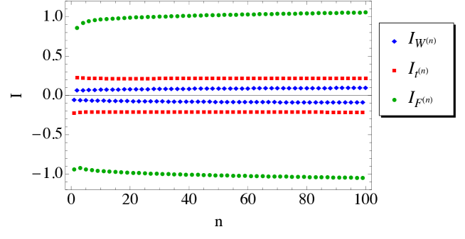
Figure 1: Behaviors of $I_{W^{(n)}}=g_{HW^{(n)}W^{(n)}}/g_{w}m_{W^{(n)}}\cos\theta_{H}$, $I_{t^{(n)}}=y_{Ht^{(n)}t^{(n)}}/y_{t}^{\text{SM}}\cos\theta_{H}$ and $I_{F^{(n)}}=y_{HF^{(n)}F^{(n)}}/y_{t}^{\text{SM}}\sin\frac{\theta_{H}}{2}$ in the case of $n_{F}=4$, $z_{L}=10^{5}$ for which $\theta_{H}=0.1153$.

In Fig. 1, the values of $I_{W^{(n)}}$, $I_{t^{(n)}}$ and $I_{F^{(n)}}$ by the numerical calculation in the $N_{F}=4$ and $\theta_{H}=0.1153$ case are shown. They approximately behave as

$$I_{W^{(n)}}\simeq(-1)^{n}\big{\{}0.0759-0.0065\ln n+0.0022(\ln n)^{2}\big{\}}~{},$$

$$I_{t^{(n)}}\simeq(-1)^{n}\big{\{}0.2304-0.0108\ln n+0.0017(\ln n)^{2}\big{\}}~{},$$

$$I_{F^{(n)}}\simeq(-1)^{n}\big{\{}1.0341-0.0457\ln n+0.0108(\ln n)^{2}\big{\}}~{}~{}$$ (3.7)

for $50\leq n\leq 200$. Note that the sign alternates in $n$. As the masses of the KK modes of the $W$ boson, top quark and dark fermion are $m_{n}\simeq n\cdot m_{\rm KK}/2$, the sum in each $\mathcal{F}$ behaves as $\sum(-1)^{n}(\ln n)^{\alpha}/n$ ($\alpha=0,1,2$) and converges. Moreover the contributions from $n\geq 1$ are suppressed by the ratio of the electroweak scale to the KK scale. Hence the ratio of $\mathcal{F}$ to the zero-mode contribution becomes

$$\frac{\mathcal{F}_{W}}{\mathcal{F}_{W^{(0)}\text{only}}}= \quad 0.9997~{},$$ (3.8)

$$\frac{\mathcal{F}_{t}}{\mathcal{F}_{t^{(0)}\text{only}}}= \quad 0.9983~{},$$ (3.9)

$$\frac{\mathcal{F}_{F}}{\mathcal{F}_{t^{(0)}\text{only}}}= -0.0032~{},$$ (3.10)

for $\theta_{H}=0.114$ and $n_{F}=4$. The ratio of the amplitude to that with only zero modes is

$$\frac{\mathcal{F}_{W}+\frac{4}{3}\mathcal{F}_{t}+4\mathcal{F}_{F}}{\mathcal{F}_{W^{(0)}\text{only}}+\frac{4}{3}\mathcal{F}_{t^{(0)}\text{only}}}=1.0027.$$ (3.11)

It is found that the contributions of the KK modes are less than 1% and negligible. The couplings of the zero modes are approximately given by $g_{HWW}\simeq g_{HWW}^{{\rm SM}}\cos\theta_{H}=g_{w}m_{W}\cos\theta_{H}$ and $y_{t}\simeq y_{t}^{{\rm SM}}\cos\theta_{H}$. Therefore the decay rate in the GHU is approximately $\cos^{2}\theta_{H}$ times that in the SM. The deviation from the SM amounts only $1\%$ for $\theta_{H}\sim 0.1$.

3.2 Gauge boson loops

The decay process $H\to Z\gamma$ is more involved than $H\to\gamma\gamma$. The KK number need not be conserved at the $Z$ and $H$ vertices, and $W_{R}^{(n)}$ also participates.

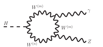
(a)

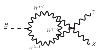
(b)

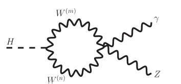
(c)

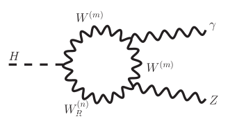
(d)

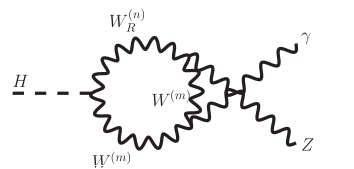
(e)

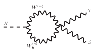
(f)

Figure 2: The gauge boson loop processes for $H\to Z\gamma$ in the $SO(5)\times U(1)$ gauge-Higgs unification. $W_{R}$ is the $SU(2)_{R}$ gauge boson and has no zero mode. Since $HW_{R}^{(m)}W_{R}^{(n)}$ couplings vanish, there are no diagrams involving two or more $W_{R}$’ s.

The gauge boson loop processes for $H\to Z\gamma$ are shown in Fig. 2. We note that $HW_{R}^{(m)}W_{R}^{(n)}$ couplings vanish. The amplitude of $W$ boson loop Figs. 2(a)(b)(c) is given in the unitary gauge by

$$\hskip-28.45274pti\mathcal{M}^{(a)}_{W^{(m)},W^{(n)}}+i\mathcal{M}^{(b)}_{W^{(m)},W^{(n)}}+i\mathcal{M}^{(c)}_{W^{(m)},W^{(n)}}$$ (3.12)

$$\hskip-28.45274pt=eg_{HW^{(m)}W^{(n)}}g_{ZW^{(m)}W^{(n)}}\epsilon^{*}_{\mu}(k_{1})\epsilon^{*}_{\nu}(k_{2})\int\frac{d^{4}p}{(2\pi)^{4}}\,D_{\tau\alpha}(p,m_{W^{(m)}}){D_{\sigma}}^{\tau}(p-k_{1}-k_{2},m_{W^{(n)}})$$ (3.13)

$$\hskip 0.0pt\times\Big{[}2D_{\beta\rho}(p-k_{1},m_{W^{(m)}})\big{\{}2\eta^{\alpha\beta}p^{\mu}-\eta^{\beta\mu}(p-2k_{1})^{\alpha}-\eta^{\alpha\mu}(p+k_{1})^{\beta}\big{\}}$$ (3.14)

$$\hskip 42.67912pt\times\big{\{}2\eta^{\rho\sigma}(p-k_{1})^{\nu}-\eta^{\sigma\nu}(p-k_{1}-2k_{2})^{\rho}-\eta^{\rho\nu}(p-k_{1}+k_{2})^{\sigma}\big{\}}$$ (3.15)

$$\hskip 14.22636pt-(2\eta^{\mu\nu}\eta^{\alpha\sigma}-\eta^{\mu\alpha}\eta^{\nu\sigma}-\eta^{\mu\sigma}\eta^{\nu\alpha})\Big{]}~{},$$ (3.16)

$$\hskip 0.0ptD_{\mu\nu}(p,m)=\Big{(}\eta_{\mu\nu}-\frac{p_{\mu}p_{\nu}}{m^{2}}\Big{)}\frac{1}{p^{2}-m^{2}+i\epsilon}~{},$$ (3.17)

where $k_{1}$ and $k_{2}$ are the photon and the $Z$ boson momenta, respectively. The amplitude (3.17) itself is divergent. However, by adding the $m\leftrightarrow n$ diagrams and using $g_{HW^{(m)}W^{(n)}}=g_{HW^{(n)}W^{(m)}}$ and $g_{ZW^{(m)}W^{(n)}}=g_{ZW^{(n)}W^{(m)}}$, the amplitude becomes

$$i \big{\{}\mathcal{M}^{(a)}_{W^{(m)},W^{(n)}}+\mathcal{M}^{(b)}_{W^{(m)},W^{(n)}}+\mathcal{M}^{(c)}_{W^{(m)},W^{(n)}}+(m\longleftrightarrow n)\big{\}}$$

$$= eg_{HW^{(m)}W^{(n)}}g_{ZW^{(m)}W^{(n)}}\epsilon^{*}_{\mu}(k_{1})\epsilon^{*}_{\nu}(k_{2})\left(\eta^{\mu\nu}-\frac{k_{2}^{\mu}k_{1}^{\nu}}{k_{1}\cdot k_{2}}\right)\frac{i}{16\pi^{2}}\frac{1}{m_{W^{(m)}}^{2}m_{W^{(n)}}^{2}}$$

$$\times\Big{\{}\Big{(}m_{W^{(m)}}^{4}+m_{W^{(n)}}^{4}+10m_{W^{(m)}}^{2}m_{W^{(n)}}^{2}\Big{)}E_{+}(m_{W^{(m)}},m_{W^{(n)}})$$

$$\quad+\Big{(}(m_{W^{(m)}}^{2}+m_{W^{(n)}}^{2})(m_{H}^{2}-m_{Z}^{2})-m_{H}^{2}m_{Z}^{2}\Big{)}E_{-}(m_{W^{(m)}},m_{W^{(n)}})$$

$$\quad-\left(4m_{W^{(m)}}^{2}m_{W^{(n)}}^{2}(m_{H}^{2}-m_{Z}^{2})+2m_{Z}^{4}(m_{W^{(m)}}^{2}+m_{W^{(n)}}^{2})\right)$$

$$\qquad\times\left(C_{0}(m_{W^{(m)}},m_{W^{(n)}})+C_{0}(m_{W^{(n)}},m_{W^{(m)}})\right)\Big{\}}$$ (3.18)

where

$$C_{0}(m_{1}^{2},m_{2}^{2}) \equiv C_{0}(0,m_{H}^{2},m_{Z}^{2},m_{1}^{2},m_{1}^{2},m_{2}^{2})~{},$$

$$E_{\pm}(m_{1},m_{2}) \equiv 1+\frac{m_{Z}^{2}}{m_{H}^{2}-m_{Z}^{2}}\left\{B_{0}(m_{H}^{2},m_{1}^{2},m_{2}^{2})-B_{0}(m_{Z}^{2},m_{1}^{2},m_{2}^{2})\right\}$$

$$\quad\pm\left\{m_{1}^{2}C_{0}(m_{1}^{2},m_{2}^{2})+m_{2}^{2}C_{0}(m_{2}^{2},m_{1}^{2})\right\}~{},$$ (3.19)

with the Passarino-Veltman functions[28, 29] defined by

$$\hskip-28.45274ptB_{0}(k^{2},m_{1}^{2},m_{2}^{2})\equiv\frac{(2\pi)^{4-D}}{i\pi^{2}}\int d^{D}q\frac{1}{(q^{2}-m_{1}^{2})\{(q+k)^{2}-m_{2}^{2}\}}~{},$$ (3.20)

$$\hskip-28.45274ptC_{0}(k_{1}^{2},(k_{1}-k_{2})^{2},k_{2}^{2},m_{1}^{2},m_{2}^{2},m_{3}^{2})$$ (3.21)

$$\hskip 0.0pt\equiv\frac{1}{i\pi^{2}}\int d^{D}q\frac{1}{(q^{2}-m_{1}^{2})\{(q+k_{1})^{2}-m_{2}^{2}\}\{(q+k_{2})^{2}-m_{3}^{2}\}}~{},$$ (3.22)

For all $C_{0}$ and $E_{\pm}$, the $D\rightarrow 4$ limit has been safely taken, so that the amplitude (3.18) is finite.

Table 1: $J_{W^{(m)}W^{(n)}}$ defined in (3.23) is shown for $0\leq m,n\leq 7$ and for $101\leq m,n\leq 108$ in the $N_{F}=4$, $z_{L}=10^{5}$ case. Only the values larger than that of $O(10^{-4})$ are shown with three significant figures.

	0	1	2	3	4	5	6	7
0	1.00	$O(10^{-4})$	$O(10^{-9})$	$O(10^{-6})$	$O(10^{-11})$	$O(10^{-8})$	$O(10^{-12})$	$O(10^{-9})$
1	$O(10^{-4})$	-0.0580	0.0595	$O(10^{-6})$	$O(10^{-5})$	$O(10^{-10})$	$O(10^{-7})$	$O(10^{-9})$
2	$O(10^{-9})$	0.0595	0.0218	-0.0413	$O(10^{-8})$	$O(10^{-5})$	$O(10^{-9})$	$O(10^{-5})$
3	$O(10^{-6})$	$O(10^{-6})$	-0.0413	-0.0625	0.0637	$O(10^{-6})$	$O(10^{-5})$	$O(10^{-10})$
4	$O(10^{-11})$	$O(10^{-5})$	$O(10^{-8})$	0.0637	0.0226	-0.0432	$O(10^{-7})$	$O(10^{-5})$
5	$O(10^{-8})$	$O(10^{-10})$	$O(10^{-5})$	$O(10^{-6})$	-0.0432	-0.0652	0.0648	$O(10^{-6})$
6	$O(10^{-12})$	$O(10^{-7})$	$O(10^{-9})$	$O(10^{-5})$	$O(10^{-7})$	0.0648	0.0233	-0.0434
7	$O(10^{-9})$	$O(10^{-9})$	$O(10^{-5})$	$O(10^{-10})$	$O(10^{-5})$	$O(10^{-6})$	-0.0434	-0.0673

	101	102	103	104	105	106	107	108
101	-0.0932	0.0705	$O(10^{-6})$	$O(10^{-4})$	$O(10^{-12})$	$O(10^{-5})$	$O(10^{-8})$	$O(10^{-6})$
102	0.0705	0.0328	-0.0406	$O(10^{-6})$	$O(10^{-4})$	$O(10^{-12})$	$O(10^{-5})$	$O(10^{-9})$
103	$O(10^{-6})$	-0.0406	-0.0934	0.0706	$O(10^{-6})$	$O(10^{-4})$	$O(10^{-12})$	$O(10^{-5})$
104	$O(10^{-4})$	$O(10^{-6})$	0.0706	0.0329	-0.0405	$O(10^{-6})$	$O(10^{-4})$	$O(10^{-12})$
105	$O(10^{-12})$	$O(10^{-4})$	$O(10^{-6})$	-0.0405	-0.0937	0.0706	$O(10^{-6})$	$O(10^{-4})$
106	$O(10^{-5})$	$O(10^{-12})$	$O(10^{-4})$	$O(10^{-6})$	0.0706	0.0330	-0.0405	$O(10^{-6})$
107	$O(10^{-8})$	$O(10^{-5})$	$O(10^{-12})$	$O(10^{-4})$	$O(10^{-6})$	-0.0405	-0.0940	0.0707
108	$O(10^{-6})$	$O(10^{-9})$	$O(10^{-5})$	$O(10^{-12})$	$O(10^{-4})$	$O(10^{-6})$	0.0707	0.0331

To obtain the amplitude quantitatively, the numerical values of the couplings $g_{HW^{(m)}W^{(n)}}$ and $g_{ZW^{(m)}W^{(n)}}$ have to be evaluated. The details of evaluation and results are summarised in Appendix. It is convenient to define the dimensionless coupling $J_{W^{(m)}W^{(n)}}$ by

$$J_{W^{(m)}W^{(n)}}\equiv\frac{g_{HW^{(m)}W^{(n)}}g_{ZW^{(m)}W^{(n)}}}{g_{w}^{2}\cos\theta_{W}\cos\theta_{H}\sqrt{m_{W^{(m)}}m_{W^{(n)}}}}~{}.$$ (3.23)

The value of $J_{W^{(m)}W^{(n)}}$ is tabulated in Table 1. It is seen that $J_{W^{(m)}W^{(n)}}$ with $|m-n|\geq 2$ is smaller than $J_{W^{(n)}W^{(n)}}$ by a factor $10^{-2}$, whereas $J_{W^{(n\pm 1)}W^{(n)}}$ and $J_{W^{(n)}W^{(n)}}$ are of the same order.

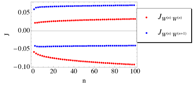
Figure 3: $J_{W^{(n)}W^{(n)}}$ and $J_{W^{(n)}W^{(n+1)}}$ are plotted for $1\leq n\leq 100$ in the $N_{F}=4$, $z_{L}=10^{5}$ case. The red circles and blue squares represent $J_{W^{(n)}W^{(n)}}$ and $J_{W^{(n)}W^{(n+1)}}$, respectively.

$J_{W^{(n)}W^{(n)}}$ and $J_{W^{(n)}W^{(n+1)}}$ are plotted in Fig. 3 for $1\leq n\leq 100$ in the $N_{F}=4$, $z_{L}=10^{5}$ case. $J_{W^{(n)}W^{(n)}}$ and $J_{W^{(n)}W^{(n+1)}}$ for $101\leq n\leq 200$ are approximately given by

$$\hskip-28.45274ptJ_{W^{(n)}W^{(n)}}\simeq-0.0272+0.00320(\ln n)-0.00083(\ln n)^{2}$$ (3.24)

$$\hskip 28.45274pt+(-1)^{n-1}\left(-0.0563+0.00654(\ln n)-0.00173(\ln n)^{2}\right)~{},$$ (3.25)

$$\hskip-28.45274ptJ_{W^{(n)}W^{(n+1)}}\simeq 0.0135-0.00160(\ln n)+0.00041(\ln n)^{2}$$ (3.26)

$$\hskip 28.45274pt+(-1)^{n-1}\left(0.0567-0.00106(\ln n)+0.00018(\ln n)^{2}\right)~{}.$$ (3.27)

Next we examine the asymptotic behavior of the amplitude for $m,n\gg 1$. The whole amplitude of the $W$ boson loop is

$$i\mathcal{M}_{W}= \frac{i}{2}\sum_{m,n}^{\infty}\Big{\{}\mathcal{M}^{(a)}_{W^{(m)},W^{(n)}}+\mathcal{M}^{(b)}_{W^{(m)},W^{(n)}}+\mathcal{M}^{(c)}_{W^{(m)},W^{(n)}}+(n\longleftrightarrow m)\Big{\}}~{}.$$ (3.28)

The diagonal part of the amplitude in (3.28) for $n\gg 1$ is rewritten as

$$i\mathcal{M}^{(a)}_{W^{(n)},W^{(n)}}+i\mathcal{M}^{(b)}_{W^{(n)},W^{(n)}}+i\mathcal{M}^{(c)}_{W^{(n)},W^{(n)}}$$

$$= eg_{w}^{2}\cos\theta_{W}\cos\theta_{H}\epsilon^{*}_{\mu}(k_{1})\epsilon^{*}_{\nu}(k_{2})\left(\eta^{\mu\nu}-\frac{k_{2}^{\mu}k_{1}^{\nu}}{k_{1}\cdot k_{2}}\right)\frac{i}{16\pi^{2}}\frac{J_{W^{(n)}W^{(n)}}}{2m_{W^{(n)}}^{3}}$$

$$\times\bigg{\{}-\frac{m_{H}^{2}-m_{Z}^{2}}{2m_{W^{(n)}}^{2}}\Big{(}12m_{W^{(n)}}^{4}+2m_{W^{(n)}}^{2}(m_{H}^{2}-m_{Z}^{2})-m_{H}^{2}m_{Z}^{2}\Big{)}I_{1}(\tau_{W^{(n)}},\lambda_{W^{(n)}})$$

$$\qquad+4\Big{(}4m_{W^{(n)}}^{2}(m_{H}^{2}-m_{Z}^{2})-m_{H}^{2}m_{Z}^{2}+m_{Z}^{4}\Big{)}I_{2}(\tau_{W^{(n)}},\lambda_{W^{(n)}})\bigg{\}},$$ (3.29)

where

$$I_{1}(a,b)=\frac{ab}{2(a-b)}+\frac{a^{2}b^{2}}{2(a-b)^{2}}\big{[}f(a)-f(b)\big{]}+\frac{a^{2}b}{(a-b)^{2}}\big{[}g(a)-g(b)\big{]},$$ (3.30)

$$I_{2}(a,b)=-\frac{ab}{2(a-b)}[f(a)-f(b)]~{},$$ (3.31)

$$g(\tau)=\begin{cases}\sqrt{\tau-1}\sin^{-1}\big{(}\sqrt{1/\tau}\big{)}&\text{for }\tau\geq 1~{},\cr\kern 5.0pt\cr\frac{1}{2}\sqrt{1-\tau}\bigg{[}\ln{\displaystyle 1+\sqrt{1-\tau}\over\displaystyle 1-\sqrt{1-\tau}}-i\pi\bigg{]}&\text{for }\tau<1~{}.\end{cases}$$ (3.32)

and $\lambda_{i}\equiv 4m_{i}^{2}/m_{Z}^{2}$. $\tau_{i}$ and $f(a)$ are defined in (3.1) and (3.4). Here, we have used

$$\frac{m_{Z}^{2}}{m_{H}^{2}-m_{Z}^{2}}\left(B_{0}(m_{H}^{2},m_{W^{(n)}}^{2},m_{W^{(n)}}^{2})-B_{0}(m_{Z}^{2},m_{W^{(n)}}^{2},m_{W^{(n)}}^{2})\right)$$ (3.33)

$$\qquad=-1-\frac{m_{H}^{2}-m_{Z}^{2}}{2m_{W^{(n)}}^{2}}I_{1}(\tau_{W^{(n)}},\lambda_{W^{(n)}})+2I_{2}(\tau_{W^{(n)}},\lambda_{W^{(n)}})~{},$$ (3.34)

$$C_{0}(0,m_{H}^{2},m_{Z}^{2},m_{W^{(n)}}^{2},m_{W^{(n)}}^{2},m_{W^{(n)}}^{2})=-\frac{1}{m_{W^{(n)}}^{2}}I_{2}(\tau_{W^{(n)}},\lambda_{W^{(n)}})~{}.$$ (3.35)

The functions $I_{1},I_{2}$ in (3.35) approach constants for $m_{W^{(n)}}\to\infty$. Since $J_{W^{(m)}W^{(n)}}$ for $|m-n|\geq 2$ are negligible comparing to $J_{W^{(m)}W^{(n)}}$ for $|m-n|\leq 1$, only the amplitude for $|m-n|\leq 1$ need to be retained. For $n\gg 1$ $m_{W^{(n\pm 1)}}\simeq m_{W^{(n)}}$ so that

$$\hskip-28.45274pt\frac{1}{2}\sum_{m}\Big{(}i\mathcal{M}^{(a)}_{W^{(m)},W^{(n)}}+i\mathcal{M}^{(b)}_{W^{(m)},W^{(n)}}+i\mathcal{M}^{(c)}_{W^{(m)},W^{(n)}}+(n\longleftrightarrow m)\Big{)}$$ (3.36)

$$\hskip-28.45274pt\simeq\;eg_{w}^{2}\cos\theta_{W}\cos\theta_{H}\epsilon^{*}_{\mu}(k_{1})\epsilon^{*}_{\nu}(k_{2})\left(\eta^{\mu\nu}-\frac{k_{2}^{\mu}k_{1}^{\nu}}{k_{1}\cdot k_{2}}\right)\frac{i}{16\pi^{2}}$$ (3.37)

$$\hskip 0.0pt\times\frac{1}{2m_{W^{(n)}}^{3}}\left(J_{W^{(n)}W^{(n)}}+J_{W^{(n+1)}W^{(n)}}+J_{W^{(n-1)}W^{(n)}}\right)$$ (3.38)

$$\hskip 0.0pt\times\bigg{\{}-\frac{m_{H}^{2}-m_{Z}^{2}}{2m_{W^{(n)}}^{2}}\Big{(}12m_{W^{(n)}}^{4}+2m_{W^{(n)}}^{2}(m_{H}^{2}-m_{Z}^{2})-m_{H}^{2}m_{Z}^{2}\Big{)}I_{1}(\tau_{W^{(n)}},\lambda_{W^{(n)}})$$ (3.39)

$$\hskip 0.0pt\qquad+4\Big{(}4m_{W^{(n)}}^{2}(m_{H}^{2}-m_{Z}^{2})-m_{H}^{2}m_{Z}^{2}+m_{Z}^{4}\Big{)}I_{2}(\tau_{W^{(n)}},\lambda_{W^{(n)}})\bigg{\}}$$ (3.40)

$$\hskip-28.45274pt\approx\;\text{const.}\times\frac{1}{n}\left(J_{W^{(n)}W^{(n)}}+J_{W^{(n+1)}W^{(n)}}+J_{W^{(n-1)}W^{(n)}}\right).$$ (3.41)

Therefore the large $n$ part of the sum in the whole amplitude of $W$ boson loop is approximated as

$$i\mathcal{M}_{W}\approx\sum_{n}^{\infty}\text{const.}\times\frac{1}{n}\left(J_{W^{(n)}W^{(n)}}+J_{W^{(n+1)}W^{(n)}}+J_{W^{(n-1)}W^{(n)}}\right).$$ (3.42)

Even though the sums $\sum J_{W^{(n)}W^{(n)}}/n$ and $\sum J_{W^{(n\pm 1)}W^{(n)}}/n$ diverge individually, the combination $\sum\left(J_{W^{(n)}W^{(n)}}+J_{W^{(n+1)}W^{(n)}}+J_{W^{(n-1)}W^{(n)}}\right)/n$ converges since

$$J_{W^{(n)}W^{(n)}}+J_{W^{(n+1)}W^{(n)}}+J_{W^{(n-1)}W^{(n)}}$$

$$\simeq(-1)^{n-1}\big{\{}-0.0563+0.00654(\ln n)-0.00173(\ln n)^{2}\big{\}}~{}.$$ (3.43)

Next we consider the amplitudes which contain $W_{R}$ in the loop. The amplitude $i\mathcal{M}^{(d)}_{W^{(m)},W_{R}^{(n)}}+i\mathcal{M}^{(e)}_{W^{(m)},W_{R}^{(n)}}+i\mathcal{M}^{(f)}_{W^{(m)},W_{R}^{(n)}}$ is obtained from (3.17) by replacing $W^{(n)}$ by $W_{R}^{(n)}$. The dimensionless coupling $J_{W^{(m)}W^{(n)}_{R}}$ is also defined as

$$J_{W^{(m)}W^{(n)}_{R}}\equiv\frac{g_{HW^{(m)}W^{(n)}_{R}}g_{ZW^{(m)}W^{(n)}_{R}}}{g_{w}^{2}\cos\theta_{W}\sqrt{m_{W^{(m)}}m_{W^{(n)}_{R}}}}~{}.$$ (3.44)

Table 2: $J_{W^{(m)}W^{(n)}_{R}}$ in (3.44) is shown for $0\leq m\leq 7$, $1\leq n\leq 4$ and for $101\leq m\leq 108$, $51\leq n\leq 55$ in the $N_{F}=4$, $z_{L}=10^{5}$ case. Only values larger than $O(10^{-4})$ are shown explicitly with three significant figures.

					$m$
		0	1	2	3	4	5	6	7
	1	$O(10^{-4})$	$O(10^{-4})$	-0.0470	$O(10^{-7})$	$O(10^{-5})$	$O(10^{-10})$	$O(10^{-6})$	$O(10^{-10})$
	2	$O(10^{-6})$	$O(10^{-6})$	0.0491	$O(10^{-4})$	-0.0514	$O(10^{-7})$	$O(10^{-4})$	$O(10^{-10})$
$n$	3	$O(10^{-8})$	$O(10^{-9})$	$O(10^{-4})$	$O(10^{-6})$	0.0517	$O(10^{-4})$	-0.0523	$O(10^{-7})$
	4	$O(10^{-8})$	$O(10^{-9})$	$O(10^{-5})$	$O(10^{-9})$	$O(10^{-5})$	$O(10^{-6})$	0.0524	$O(10^{-4})$

					$m$
		101	102	103	104	105	106	107	108
	51	$O(10^{-4})$	-0.0530	$O(10^{-6})$	$O(10^{-4})$	$O(10^{-13})$	$O(10^{-5})$	$O(10^{-9})$	$O(10^{-6})$
	52	$O(10^{-6})$	0.0532	$O(10^{-4})$	-0.0530	$O(10^{-6})$	$O(10^{-4})$	$O(10^{-13})$	$O(10^{-5})$
$n$	53	$O(10^{-11})$	$O(10^{-4})$	$O(10^{-6})$	0.0532	$O(10^{-4})$	-0.0530	$O(10^{-6})$	$O(10^{-4})$
	54	$O(10^{-8})$	$O(10^{-5})$	$O(10^{-11})$	$O(10^{-4})$	$O(10^{-6})$	0.0532	$O(10^{-4})$	-0.0530
	55	$O(10^{-12})$	$O(10^{-6})$	$O(10^{-8})$	$O(10^{-5})$	$O(10^{-11})$	$O(10^{-4})$	$O(10^{-6})$	0.0532

As is seen in the Table 2 , $J_{W^{(m)}W^{(n)}_{R}}$ is appreciable only when $m/2-n=0,1$. Note that $m_{W_{R}^{(n)}}\simeq n\cdot m_{\rm KK}$ while $m_{W^{(n)}}\simeq n\cdot m_{\rm KK}/2$. For $m/2-n=0,1$, $m_{W^{(m)}}\simeq m_{W^{(n)}}\simeq n\cdot m_{\rm KK}$ is satisfied. Hence the whole amplitude of the $W$-$W_{R}$ boson loop is

$$i\mathcal{M}_{W_{R}} =\sum_{m,n}^{\infty}\Big{(}i\mathcal{M}^{(d)}_{W^{(m)},W^{(n)}_{R}}+i\mathcal{M}^{(e)}_{W^{(m)},W^{(n)}_{R}}+i\mathcal{M}^{(f)}_{W^{(m)},W^{(n)}_{R}}$$

$$\quad\qquad+i\mathcal{M}^{(d)}_{W^{(n)}_{R},W^{(m)}}+i\mathcal{M}^{(e)}_{W^{(n)}_{R},W^{(m)}}+i\mathcal{M}^{(f)}_{W^{(n)}_{R},W^{(m)}}\Big{)}$$

$$\approx\sum_{n}^{\infty}\text{const.}\times\frac{1}{n}\left(J_{W^{(n)}W^{(n/2)}_{R}}+J_{W^{(n)}W^{(n/2+1)}_{R}}\right)~{}.$$ (3.45)

$J_{W^{(n)}W_{R}^{(n/2)}}$ and $J_{W^{(n)}W_{R}^{(n/2+1)}}$ are plotted in Fig. 4 for $1\leq n\leq 100$ in the $N_{F}=4$, $z_{L}=10^{5}$ case. $J_{W^{(n)}W_{R}^{(n/2)}}$ and $J_{W^{(n)}W_{R}^{(n/2+1)}}$ are approximated in this range by

$$J_{W^{(n)}W_{R}^{(n/2)}} \simeq-0.0530-0.000018(\ln n)+4.4\times 10^{-6}(\ln n)^{2}$$

$$J_{W^{(n)}W_{R}^{(n/2+1)}} \simeq\hskip 8.00003pt0.0530+0.000054(\ln n)-3.7\times 10^{-6}(\ln n)^{2}.$$ (3.46)

$J_{W^{(n)}W_{R}^{(n/2)}}+J_{W^{(n)}W_{R}^{(n/2+1)}}$ is small, and almost vanishes within numerical errors.

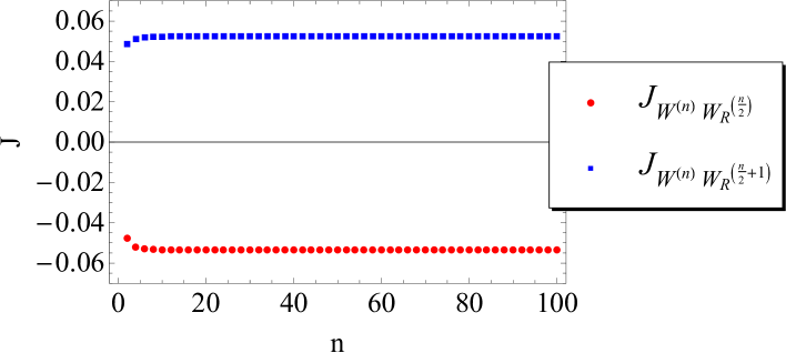
Figure 4: $J_{W^{(n)}W_{R}^{(n/2)}}$ and $J_{W^{(n)}W_{R}^{(n/2+1)}}$ are plotted for $1\leq n\leq 100$ in the $N_{F}=4$, $z_{L}=10^{5}$ case. The red circles and blue squares represent $J_{W^{(n)}W_{R}^{(n/2)}}$ and $J_{W^{(n)}W_{R}^{(n/2+1)}}$, respectively.

3.3 Fermion loops

Contributions of fermion loops to $\Gamma(H\to Z\gamma)$ are evaluated similarly. Top quark, charged dark fermions and their KK excitations give substantial contributions as shown in Fig. 5, whereas contributions from other quarks and leptons are negligible.

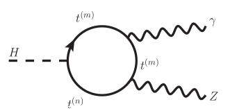
(a)

(b)

(c)

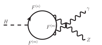
(d)

Figure 5: The fermion loop processes of $H\to Z\gamma$ decay in the $SO(5)\times U(1)$ gauge-Higgs unification. $F^{+}$ is the charged dark fermion which does not have a zero mode.

The diagrams of fermion loops Fig. 5 (a, b) (or (c,d)), with generic fermions $f^{(m)}$, yield

$$\hskip-28.45274pti\mathcal{M}^{(a)}_{f^{(m)},f^{(n)}}+i\mathcal{M}^{(b)}_{f^{(m)},f^{(n)}}$$ (3.47)

$$\hskip-28.45274pt=-Q_{f}e\,\epsilon_{\mu}^{*}(k_{1})\epsilon_{\nu}^{*}(k_{2})\int\frac{d^{4}p}{(2\pi)^{4}}\frac{1}{p^{2}-m_{f^{(m)}}^{2}}\frac{1}{(p-k_{1})^{2}-m_{f^{(m)}}^{2}}\frac{1}{(p-k_{1}-k_{2})^{2}-m_{f^{(n)}}^{2}}$$ (3.48)

$$\hskip 0.0pt\times{\rm Tr\,}\Big{[}\big{(}y_{f^{(m)}f^{(n)}}+\hat{y}_{f^{(m)}f^{(n)}}\gamma^{5}\big{)}(/\kern-5.0ptp+m_{f^{(m)}})\gamma^{\mu}(/\kern-5.0ptp-/\kern-5.0ptk_{1}+m_{f^{(m)}})\gamma^{\nu}$$ (3.49)

$$\hskip 28.45274pt\times\big{(}g^{V}_{Zf^{(m)}f^{(n)}}+g^{A}_{Zf^{(m)}f^{(n)}}\gamma^{5}\big{)}(/\kern-5.0ptp-/\kern-5.0ptk_{1}-/\kern-5.0ptk_{2}+m_{f^{(n)}})$$ (3.50)

$$\hskip 0.0pt+\big{(}y_{f^{(m)}f^{(n)}}+\hat{y}_{f^{(n)}f^{(m)}}\gamma^{5}\big{)}(-/\kern-5.0ptp+/\kern-5.0ptk_{1}+/\kern-5.0ptk_{2}+m_{f^{(n)}})\gamma^{\nu}$$ (3.51)

$$\hskip 28.45274pt\times\big{(}g^{V}_{Zf^{(m)}f^{(n)}}+g^{A}_{Zf^{(n)}f^{(m)}}\gamma^{5}\big{)}(-/\kern-5.0ptp+/\kern-5.0ptk_{1}+m_{f^{(m)}})\gamma^{\mu}(-/\kern-5.0ptp+m_{f^{(m)}})\Big{]}.$$ (3.52)

The Yukawa couplings $y_{f^{(m)}f^{(n)}}$ and $\hat{y}_{f^{(m)}f^{(n)}}$ for $f^{(m)}=t^{(m)}$ and $F^{(m)}$ are given in (A.64) and (A.89), respectively. The amplitude (3.52) itself involves divergent integrals, but by adding the $m\leftrightarrow n$ diagrams and making use of $y_{f^{(m)}f^{(n)}}=y_{f^{(n)}f^{(m)}}$ and $\hat{y}_{f^{(m)}f^{(n)}}=-\hat{y}_{f^{(n)}f^{(m)}}$, one finds that

$$\hskip-28.45274pti\mathcal{M}^{(a)}_{f^{(m)},f^{(n)}}+i\mathcal{M}^{(b)}_{f^{(m)},f^{(n)}}+(m\leftrightarrow n)=-\frac{iQ_{f}e}{4\pi^{2}}\epsilon_{\mu}^{*}(k_{1})\epsilon_{\nu}^{*}(k_{2})\bigg{(}\eta^{\mu\nu}-\frac{k_{2}^{\mu}k_{1}^{\nu}}{k_{1}\cdot k_{2}}\bigg{)}$$ (3.53)

$$\hskip-14.22636pt\times\Big{\{}y_{f^{(m)}f^{(n)}}g^{V}_{Zf^{(m)}f^{(n)}}G_{+}(m_{f^{(m)}},m_{f^{(n)}})-\hat{y}_{f^{(m)}f^{(n)}}g^{A}_{Zf^{(m)}f^{(n)}}G_{-}(m_{f^{(m)}},m_{f^{(n)}})\Big{\}}~{},$$ (3.54)

$$\hskip-28.45274ptG_{\pm}(m_{1},m_{2})=2(m_{1}\pm m_{2})+\frac{2m_{Z}^{2}(m_{1}\pm m_{2})}{m_{H}^{2}-m_{Z}^{2}}\big{(}B_{0}(m_{H}^{2},m_{1}^{2},m_{2}^{2})-B_{0}(m_{Z}^{2},m_{1}^{2},m_{2}^{2})\big{)}$$ (3.55)

$$\hskip 42.67912pt+m_{1}(2m_{1}^{2}\pm 2m_{1}m_{2}-m_{H}^{2}+m_{Z}^{2})C_{0}(0,m_{H}^{2},m_{Z}^{2},m_{1}^{2},m_{1}^{2},m_{2}^{2})\$$ (3.56)

$$\hskip 42.67912pt\pm m_{2}(2m_{2}^{2}\pm 2m_{1}m_{2}-m_{H}^{2}+m_{Z}^{2})C_{0}(0,m_{H}^{2},m_{Z}^{2},m_{2}^{2},m_{2}^{2},m_{1}^{2})~{}.$$ (3.57)

In this form the amplitude is finite.

Table 3: $J_{t^{(m)}t^{(n)}}$ is shown for $0\leq m,n\leq 7$ and for $101\leq m,n\leq 108$ in the $N_{F}=4$, $z_{L}=10^{5}$ case. Only the values larger than $O(10^{-4})$ are shown with three significant figures.

	0	1	2	3	4	5	6	7
0	0.0988	-0.0041	$O(10^{-4})$	$O(10^{-5})$	$O(10^{-7})$	$O(10^{-6})$	$O(10^{-6})$	$O(10^{-7})$
1	-0.0041	-0.0790	0.0638	$O(10^{-5})$	$O(10^{-4})$	$O(10^{-9})$	$O(10^{-10})$	$O(10^{-8})$
2	$O(10^{-4})$	0.0638	-0.0350	-0.0071	$O(10^{-6})$	$O(10^{-6})$	$O(10^{-9})$	$O(10^{-5})$
3	$O(10^{-5})$	$O(10^{-5})$	-0.0071	-0.0763	0.0616	$O(10^{-6})$	$O(10^{-4})$	$O(10^{-9})$
4	$O(10^{-7})$	$O(10^{-4})$	$O(10^{-6})$	0.0616	-0.0338	-0.0071	$O(10^{-6})$	$O(10^{-6})$
5	$O(10^{-6})$	$O(10^{-9})$	$O(10^{-6})$	$O(10^{-6})$	-0.0071	-0.0754	0.0609	$O(10^{-6})$
6	$O(10^{-6})$	$O(10^{-10})$	$O(10^{-9})$	$O(10^{-4})$	$O(10^{-6})$	0.0609	-0.0334	-0.0070
7	$O(10^{-7})$	$O(10^{-8})$	$O(10^{-5})$	$O(10^{-9})$	$O(10^{-6})$	$O(10^{-6})$	-0.0070	-0.0751

	101	102	103	104	105	106	107	108
101	-0.0761	0.0610	$O(10^{-6})$	$O(10^{-4})$	$O(10^{-13})$	$O(10^{-7})$	$O(10^{-8})$	$O(10^{-6})$
102	0.0610	-0.0337	-0.0068	$O(10^{-6})$	$O(10^{-6})$	$O(10^{-13})$	$O(10^{-5})$	$O(10^{-9})$
103	$O(10^{-6})$	-0.0068	-0.0761	0.0610	$O(10^{-6})$	$O(10^{-4})$	$O(10^{-13})$	$O(10^{-7})$
104	$O(10^{-4})$	$O(10^{-6})$	0.0610	-0.0337	-0.0068	$O(10^{-6})$	$O(10^{-6})$	$O(10^{-13})$
105	$O(10^{-13})$	$O(10^{-6})$	$O(10^{-6})$	-0.0068	-0.0761	0.0610	$O(10^{-6})$	$O(10^{-4})$
106	$O(10^{-7})$	$O(10^{-13})$	$O(10^{-4})$	$O(10^{-6})$	0.0610	-0.0337	-0.0068	$O(10^{-6})$
107	$O(10^{-8})$	$O(10^{-5})$	$O(10^{-13})$	$O(10^{-6})$	$O(10^{-6})$	-0.0068	-0.0762	0.0610
108	$O(10^{-6})$	$O(10^{-9})$	$O(10^{-7})$	$O(10^{-13})$	$O(10^{-4})$	$O(10^{-6})$	0.0610	-0.0337

Table 4: $J_{F^{+(m)}F^{+(n)}}$ is shown for $0\leq m,n\leq 7$ and for $101\leq m,n\leq 108$ in the $N_{F}=4$, $z_{L}=10^{5}$ case. Only the values larger than $O(10^{-4})$ are shown with three significant figures.

	1	2	3	4	5	6	7
1	0.2256	-0.0272	$O(10^{-5})$	-0.0040	$O(10^{-8})$	$O(10^{-5})$	$O(10^{-7})$
2	-0.0272	0.2378	0.0824	$O(10^{-6})$	$O(10^{-5})$	$O(10^{-8})$	$O(10^{-5})$
3	$O(10^{-5})$	0.0824	0.2204	-0.3188	$O(10^{-6})$	0.0036	$O(10^{-8})$
4	-0.0040	$O(10^{-6})$	-0.3188	0.2554	0.0866	$O(10^{-6})$	$O(10^{-5})$
5	$O(10^{-8})$	$O(10^{-5})$	$O(10^{-6})$	0.0866	0.2245	-0.3263	$O(10^{-6})$
6	$O(10^{-5})$	$O(10^{-8})$	-0.0036	$O(10^{-6})$	-0.3263	0.2612	0.0874
7	$O(10^{-7})$	$O(10^{-5})$	$O(10^{-8})$	$O(10^{-5})$	$O(10^{-6})$	0.0874	0.2271

	101	102	103	104	105	106	107	108
101	0.2505	-0.3528	$O(10^{-6})$	-0.0033	$O(10^{-11})$	$O(10^{-5})$	$O(10^{-8})$	$O(10^{-5})$
102	-0.3528	0.2918	0.0848	$O(10^{-5})$	$O(10^{-5})$	$O(10^{-12})$	$O(10^{-5})$	$O(10^{-8})$
103	$O(10^{-6})$	0.0848	0.2508	-0.3531	$O(10^{-6})$	-0.0033	$O(10^{-11})$	$O(10^{-5})$
104	-0.0033	$O(10^{-5})$	-0.3530	0.2921	0.0848	$O(10^{-5})$	$O(10^{-5})$	$O(10^{-12})$
105	$O(10^{-11})$	$O(10^{-5})$	$O(10^{-6})$	0.0848	0.2510	-0.3533	$O(10^{-6})$	-0.0033
106	$O(10^{-5})$	$O(10^{-12})$	-0.0033	$O(10^{-5})$	-0.3533	0.2924	0.0847	$O(10^{-5})$
107	$O(10^{-8})$	$O(10^{-5})$	$O(10^{-11})$	$O(10^{-5})$	$O(10^{-6})$	0.0847	0.2512	-0.3535
108	$O(10^{-5})$	$O(10^{-8})$	$O(10^{-5})$	$O(10^{-12})$	-0.0033	$O(10^{-5})$	-0.3535	0.2927

We define $J_{t^{(m)}t^{(n)}}$ and $J_{F^{+(m)}F^{+(n)}}$ by

$$J_{t^{(m)}t^{(n)}} \equiv\frac{g^{V}_{Zt^{(m)}t^{(n)}}y_{t^{(m)}t^{(n)}}\cos\theta_{W}}{g_{w}y_{t}\cos\theta_{H}},$$ (3.58)

$$J_{F^{+(m)}F^{+(n)}} \equiv\frac{g^{V}_{ZF^{+(m)}F^{+(n)}}y_{F^{(m)}F^{(n)}}\cos\theta_{W}}{g_{w}y_{t}\sin\frac{\theta_{H}}{2}}$$ (3.59)

In the Table 3 and Table 4, $J_{t^{(m)}t^{(n)}}$ and $J_{F^{+(m)}F^{+(n)}}$ by the numerical evaluation are shown. As in the case of $J_{W^{(n)}W^{(n)}}$, $J_{t^{(m)}t^{(n)}}$ and $J_{F^{+(m)}F^{+(n)}}$ for $|m-n|\geq 2$ become negligible for $m,n>100$. In addition, the terms proportional to $\hat{y}_{f^{(m)}f^{(n)}}g^{A}_{Zf^{(m)}f^{(n)}}$ are negligible around $m,n=100$. The ratio $(\hat{y}_{f^{(m)}f^{(n)}}/y_{f^{(m)}f^{(n)}})\cdot(g^{A}_{Zf^{(m)}f^{(n)}}/g^{V}_{Zf^{(m)}f^{(n)}})$ is smaller than $10^{-4}$, and the $\hat{y}_{f^{(m)}f^{(n)}}g^{A}_{Zf^{(m)}f^{(n)}}$ term in (3.57) may be dropped.

For the asymptotic behavior of the amplitude for $m,n\gg 1$ only the $|m-n|\leq 1$ terms are relevant. For $|m-n|\leq 1$, $m_{f^{(n\pm 1)}}\simeq m_{f^{(n)}}$ and the amplitudes are evaluated as

$$\hskip-28.45274pti\mathcal{M}_{\text{fermion}}$$ (3.60)

$$\hskip-28.45274pt\equiv\frac{1}{2}\sum_{m,n}^{\infty}\Big{\{}i\mathcal{M}^{(a)}_{t^{(m)},t^{(n)}}+i\mathcal{M}^{(b)}_{t^{(m)},t^{(n)}}+i\mathcal{M}^{(c)}_{F^{+(m)},F^{+(n)}}+i\mathcal{M}^{(d)}_{F^{+(m)},F^{+(n)}}+(m\leftrightarrow n)\Big{\}}$$ (3.61)

$$\hskip-28.45274pt\approx\sum_{n}^{\infty}\frac{i}{4\pi^{2}}\epsilon_{\mu}^{*}(k_{1})\epsilon_{\nu}^{*}(k_{2})\bigg{(}\eta^{\mu\nu}-\frac{k_{2}^{\mu}k_{1}^{\nu}}{k_{1}\cdot k_{2}}\bigg{)}\frac{eg_{w}y_{t}\cos\theta_{H}}{\cos\theta_{W}}(m_{H}^{2}-m_{Z}^{2})$$ (3.62)

$$\hskip-28.45274pt\times\bigg{\{}\frac{2}{3m_{t^{(n)}}}(J_{t^{(n)}t^{(n)}}+J_{t^{(n+1)}t^{(n)}}+J_{t^{(n-1)}t^{(n)}})\Big{[}I_{1}(\tau_{t^{(n)}},\lambda_{t^{(n)}})-I_{2}(\tau_{t^{(n)}},\lambda_{t^{(n)}})\Big{]}$$ (3.63)

$$\hskip-14.22636pt+\frac{1}{m_{F^{+(n)}}}(J_{F^{+(n)}F^{+(n)}}+J_{F^{+(n+1)}F^{+(n)}}+J_{F^{+(n-1)}F^{+(n)}})$$ (3.64)

$$\hskip 85.35826pt\times\Big{[}I_{1}(\tau_{F^{+(n)}},\lambda_{F^{+(n)}})-I_{2}(\tau_{F^{+(n)}},\lambda_{F^{+(n)}})\Big{]}\bigg{\}}~{}.$$ (3.65)

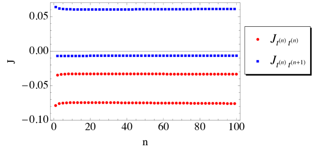
Figure 6: $J_{t^{(n)}t^{(n)}}$ and $J_{t^{(n)}t^{(n+1)}}$ are plotted for $1\leq n\leq 100$ in the $N_{F}=4$, $z_{L}=10^{5}$ case. The red circles and blue squares express $J_{t^{(n)}t^{(n)}}$ and $J_{t^{(n)}t^{(n+1)}}$, respectively.

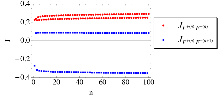
Figure 7: $J_{F^{+(n)}F^{+(n)}}$ and $J_{F^{+(n)}F^{+(n+1)}}$ are plotted for $1\leq n\leq 100$ in the $N_{F}=4$, $z_{L}=10^{5}$ case. The red circles and blue squares express $J_{F^{+(n)}F^{+(n)}}$ and $J_{F^{+(n)}F^{+(n+1)}}$, respectively.

$J_{t^{(n)}t^{(m)}}$ and $J_{F^{+(n)}F^{+(m)}}$ ($m=n,n+1$) are plotted in Figs. 6 and 7. They are approximately given, for $101\leq n\leq 200$, by

$$\hskip-28.45274ptJ_{t^{(n)}t^{(n)}}\simeq-0.0597+0.00323(\ln n)-0.00047(\ln n)^{2}$$

$$\hskip 28.45274pt+(-1)^{n-1}\big{\{}-0.0230+0.00122(\ln n)-0.00018(\ln n)^{2}\big{\}},$$

$$\hskip-28.45274ptJ_{t^{(n)}t^{(n+1)}}\simeq 0.0296-0.00162(\ln n)+0.00024(\ln n)^{2}$$

$$\hskip 28.45274pt+(-1)^{n-1}\big{\{}0.0362-0.00143(\ln n)+0.00020(\ln n)^{2}\big{\}},$$ (3.66)

$$\hskip-28.45274ptJ_{F^{+(n)}F^{+(n)}}\simeq 0.280-0.0172(\ln n)+0.00331(\ln n)^{2}$$

$$\hskip 28.45274pt+(-1)^{n-1}\big{\{}-0.0212+0.00131(\ln n)-0.00026(\ln n)^{2}\big{\}},$$

$$\hskip-28.45274ptJ_{F^{+(n)}F^{+(n+1)}}\simeq-0.138+0.0084(\ln n)-0.00163(\ln n)^{2}$$

$$\hskip 28.45274pt+(-1)^{n-1}\big{\{}-0.2218+0.00558(\ln n)-0.00107(\ln n)^{2}\big{\}}.$$ (3.67)

Adding them, one finds, within numerical errors, that

$$\hskip-28.45274ptJ_{t^{(n)}t^{(n)}}+J_{t^{(n+1)}t^{(n)}}+J_{t^{(n-1)}t^{(n)}}$$ (3.68)

$$\hskip-14.22636pt\approx(-1)^{n-1}\big{\{}-0.0230+0.00122(\ln n)-0.00018(\ln n)^{2}\big{\}},$$ (3.69)

$$\hskip-28.45274ptJ_{F^{+(n)}F^{+(n)}}+J_{F^{+(n+1)}F^{+(n)}}+J_{F^{+(n-1)}F^{+(n)}}$$ (3.70)

$$\hskip-14.22636pt\approx(-1)^{n-1}\big{\{}-0.0212+0.00131(\ln n)-0.00026(\ln n)^{2}\big{\}}.$$ (3.71)

Since $i\mathcal{M}_{f}\propto\sum_{n}(J_{f^{(n)}f^{(n)}}+J_{f^{(n+1)}f^{(n)}}+J_{f^{(n-1)}f^{(n)}})/n$ for large $n$, the sum converges as in the case of the gauge boson loops.

3.4 Total amplitude

The ratio of the sum of the all boson contributions to the $W$ boson contribution and that of all the fermion contributions to the top quark contribution are given by

$$\frac{\mathcal{M}_{\text{boson}}}{\mathcal{M}_{W^{(0)}\text{only}}}=0.9998,\quad\frac{\mathcal{M}_{\text{fermion}}}{\mathcal{M}_{t^{(0)}\text{only}}}=1.0023,$$ (3.72)

for $z_{L}=10^{5}$, $n_{F}=4$, and $\theta_{H}=0.1153$, respectively where $\mathcal{M}_{\text{boson}}\equiv\mathcal{M}_{W}+\mathcal{M}_{W_{R}}$. The ratio of the whole amplitude to the $W$ boson and top quark contributions is

$$\frac{\mathcal{M}_{\text{boson}}+\mathcal{M}_{\text{fermion}}}{\mathcal{M}_{W^{(0)}\text{only}}+\mathcal{M}_{t^{(0)}\text{only}}}=0.9997,$$ (3.73)

One finds that the KK mode contributions are negligible. As $g_{HW^{(0)}W^{(0)}}\simeq g_{w}\cos\theta_{H}$ and $y_{t^{(0)}}\simeq y_{t\text{SM}}\cos\theta_{H}$, the decay width is approximated by

$$\Gamma(H\to Z\gamma)_{\text{GHU}}\simeq\Gamma(H\to Z\gamma)_{\text{SM}}\times\cos^{2}\theta_{H}.$$ (3.74)

In the gauge-Higgs unification, the decay width of $H\to WW$, $H\to ZZ$, $H\to bb$ and $H\to\tau\tau$ are suppressed by $\cos^{2}\theta_{H}$ at the tree level. The decay width of the $H\to\gamma\gamma$ and $H\to Z\gamma$ are also suppressed by $\cos^{2}\theta_{H}$. Therefore the branching ratios of the Higgs decay modes in this model are almost the same as in the SM. The dominant process in the Higgs boson production is $gg\to H$, and the production cross section is also suppressed by $\cos^{2}\theta_{H}$. Therefore the signal strength, $\sigma(gg\to H)B(H\to Z\gamma)/[\sigma(gg\to H)B(H\to Z\gamma)]_{\rm SM}$, is approximately $\cos^{2}\theta_{H}$ as in the other decay modes. For $\theta_{H}\sim 0.1$, the deviation from the SM amounts only 1%.

We stress the finiteness of $\Gamma(H\to Z\gamma)$ in the gauge-Higgs unification which results from non-trivial cancellation among contributions of the KK modes. One might wonder why such cancellation takes place and what underlies the finiteness of the amplitude ${\cal M}(H\to Z\gamma)$ in the gauge-Higgs unification. We argue that it is guaranteed by the gauge invariance and by the fact that the 4D Higgs field $H$ is the fluctuation mode of the AB phase $\theta_{H}$. In the effective action the 4D Higgs field $H(x)$ and AB phase $\theta_{H}$ appear in the combination of $\theta_{H}+H(x)/f_{H}$ so that ${\cal M}(H\to Z\gamma)$ is related to $(\partial/\partial\theta_{H})\Pi_{Z\gamma}(\theta_{H})$ where $\Pi_{Z\gamma}(\theta_{H})$ is the $Z\gamma$ vacuum polarization. The 5D gauge invariance guarantees that $\Pi_{Z\gamma}(\theta_{H})$ is periodic in $\theta_{H}$, and can be expanded in a Fourier series $\Pi_{Z\gamma}(\theta_{H})=\sum_{n}\alpha_{n}e^{in\theta_{H}}$. The $\theta_{H}$-dependence of the $Z$ couplings of the fields running the inside loops is known to be very weak. At the one loop level the dominant $\theta_{H}$-dependence of $\Pi_{Z\gamma}(\theta_{H})$ comes from the propagators inside the loop. Hence the divergence degree is lowered by differentiating $\Pi_{Z\gamma}(\theta_{H})$ with respect to $\theta_{H}$. There should exist a positive integer $q$ such that $\partial^{q}\Pi_{Z\gamma}/\partial\theta_{H}^{q}=\sum_{n\not=0}(in)^{q}\alpha_{n}e^{in\theta_{H}}$ is finite. This in turn implies that $\Pi_{Z\gamma}(\theta_{H})-\alpha_{0}$ is finite, from which the finiteness of ${\cal M}(H\to Z\gamma)$ at the one loop level follows. A similar argument has been employed to prove the finiteness of the effective potential $V_{\rm eff}(\theta_{H})$ at the one loop level.[30]

4 Conclusion and discussions

In this paper we have evaluated the decay rate $\Gamma(H\to Z\gamma)$ in the $SO(5)\times U(1)$ gauge-Higgs unification. The processes $H\to\gamma\gamma$ and $H\to Z\gamma$ do not occur at the tree level. They do proceed at the one loop level, where an infinite number of the KK modes of gauge bosons and fermions give loop corrections. Contrary to the naive expectation that the sum of an infinite number of the KK mode contributions may yield substantial corrections to the decay rates in the SM, it has been known that the correction to $\Gamma(H\to\gamma\gamma)$ coming from KK modes turns out very tiny, thanks to the cancellation among the KK mode corrections.

We have examined the process $H\to Z\gamma$ in detail, for which the KK number need not be conserved inside the loop. We have shown, by direct evaluation, that there appears miraculous cancellation among the loop diagrams in which the KK number is conserved in the loop and those in which the KK number is not conserved. As a result the amplitude for $H\to Z\gamma$ becomes finite. We also showed that the correction due to various KK modes is very small. $\Gamma(H\to Z\gamma)$ in the gauge-Higgs unification is approximately $\cos^{2}\theta_{H}$ times that in the SM. The deviation from the SM is very small for $\theta_{H}<0.1$.

The result is very promising. The $SO(5)\times U(1)$ gauge-Higgs unification yields almost the same phenomenology as the SM at low energies. At higher energy scale it predicts KK excitation modes as $Z^{\prime}$ and $W^{\prime}$ events and a dark matter candidate, which awaits confirmation at 14 TeV LHC and by DM direct-detection experiments. Small deviations of $HWW$ and $HZZ$ couplings from the SM will be checked in future colliders.[31] In addition to deriving more predictions for collider experiments, the scenario of the gauge-Higgs unification has to be refined. The scenario of the gauge-Higgs grand unification has been proposed.[32] An attempt has been made to dynamically determine orbifold boundary conditions.[33] The Hosotani mechanism, essential for the electroweak gauge symmetry breaking in the gauge-Higgs unification, has been investigated nonperturbatively on the lattice.[34] The gauge-Higgs unification is one of the keys to investigate the extra dimension.

Acknowledgements

This work was supported in part by Japan Society for the Promotion of Science, Grants-in-Aid for Scientific Research, No. 23104009 (YH), No. 21244036 (YH), and National Research Foundation of Korea, 2012R1A2A1A01006053 (HH).

Appendix A Couplings of KK modes to $Z$ and $H$

We summarize the $Z$ and $H$ couplings of the KK modes relevant for $H\rightarrow Z\gamma$.

A.1 Base functions

Mode functions for KK towers of various fields in the RS spacetime are expressed in terms of Bessel functions. For gauge fields we define

$$\hskip-28.45274ptC(z;\lambda)=\frac{\pi}{2}\lambda zz_{L}F_{1,0}(\lambda z,\lambda z_{L})~{},\quad C^{\prime}(z;\lambda)=\frac{\pi}{2}\lambda^{2}zz_{L}F_{0,0}(\lambda z,\lambda z_{L})~{},$$ (A.1)

$$\hskip-28.45274ptS(z;\lambda)=-\frac{\pi}{2}\lambda zF_{1,1}(\lambda z,\lambda z_{L})~{},\quad S^{\prime}(z;\lambda)=-\frac{\pi}{2}\lambda^{2}zF_{0,1}(\lambda z,\lambda z_{L})~{},$$ (A.2)

$$\hskip-28.45274pt\hat{S}(z;\lambda)=\frac{C(1;\lambda)}{S(1;\lambda)}\,S(z;\lambda)~{},$$ (A.3)

where $F_{\alpha,\beta}(u,v)=J_{\alpha}(u)Y_{\beta}(v)-Y_{\alpha}(u)J_{\beta}(v)$. They satisfy

$$\hskip-28.45274ptC(z_{L};\lambda)=z_{L}~{},~{}~{}C^{\prime}(z_{L};\lambda)=0~{},~{}~{}S(z_{L};\lambda)=0~{},~{}~{}S^{\prime}(z_{L};\lambda)=\lambda~{},$$ (A.4)

$$\hskip-28.45274ptCS^{\prime}-SC^{\prime}=\lambda z~{}.$$ (A.5)

For fermions with a bulk mass parameter $c$ we define

$$\hskip-28.45274pt\begin{pmatrix}C_{L}\cr S_{L}\end{pmatrix}(z;\lambda,c)=\pm\frac{\pi}{2}\lambda\sqrt{zz_{L}}F_{c+{1\over 2},c\mp{1\over 2}}(\lambda z,\lambda z_{L})~{},$$ (A.6)

$$\hskip-28.45274pt\begin{pmatrix}C_{R}\cr S_{R}\end{pmatrix}(z;\lambda,c)=\mp\frac{\pi}{2}\lambda\sqrt{zz_{L}}F_{c-{1\over 2},c\pm{1\over 2}}(\lambda z,\lambda z_{L})~{}.$$ (A.7)

They satisfy

$$\hskip-28.45274ptD_{+}(c)\begin{pmatrix}C_{L}\cr S_{L}\end{pmatrix}=\lambda\begin{pmatrix}S_{R}\cr C_{R}\end{pmatrix}~{},~{}~{}D_{-}(c)\begin{pmatrix}C_{R}\cr S_{R}\end{pmatrix}=\lambda\begin{pmatrix}S_{L}\cr C_{L}\end{pmatrix}~{},$$ (A.8)

$$\hskip 28.45274ptD_{\pm}(c)=\pm\frac{d}{dz}+\frac{c}{z}~{},$$ (A.9)

$$\hskip-28.45274ptC_{R}=C_{L}=1~{},~{}~{}S_{R}=S_{L}=0~{},~{}~{}{\rm at~{}}z=z_{L}~{},$$ (A.10)

$$\hskip-28.45274ptC_{L}C_{R}-S_{L}S_{R}=1~{}.$$ (A.11)

In the following we evaluate various couplings by inserting the formulas for the KK expansions. Basic formulas for the KK expansions of gauge fields and quark fields are summarized in Ref. [24], whereas those for dark fermions are given in Ref. [25]. We adopt the same notation as in those references. The numerical values for the various couplings are given for the parameter set

$$z_{L}=10^{5},\theta_{H}=0.1153,m_{\text{KK}}=7.405\text{ TeV},k=2.357\times 10^{8}\text{ GeV},c_{t}=0.2270,c_{F}=0.3321.$$ (A.12)

A.2 $ZW^{(m)}W^{(n)}$ coupling

The $ZW^{(m)}W^{(n)}$ coupling is contained in

$$\int_{1}^{z_{L}}\frac{dz}{kz}\left(-\frac{1}{4}\right)\text{Tr}\left[F_{\mu\nu}F_{\rho\sigma}\right]\eta^{\mu\rho}\eta^{\nu\sigma}$$ (A.13)

$$\supset ig_{A}\int_{1}^{z_{L}}\frac{dz}{kz}\text{Tr}\Big{[}(\partial_{\mu}\hat{Z}_{\nu}-\partial_{\nu}\hat{Z}_{\mu})[\hat{W}^{+}_{\rho},\hat{W}^{-}_{\sigma}]$$ (A.14)

$$\qquad+(\partial_{\mu}\hat{W}^{-}_{\nu}-\partial_{\nu}\hat{W}^{-}_{\mu})[\hat{Z}_{\rho},\hat{W}^{+}_{\sigma}]+(\partial_{\mu}\hat{W}^{+}_{\nu}-\partial_{\nu}\hat{W}^{+}_{\mu})[\hat{Z}_{\rho},\hat{W}^{-}_{\sigma}]\Big{]}\eta^{\mu\rho}\eta^{\nu\sigma}$$

$$\supset i\sum_{m,n}g_{ZW^{(m)}W^{(n)}}\eta^{\mu\rho}\eta^{\nu\sigma}\Big{\{}(\partial_{\mu}Z_{\nu}-\partial_{\nu}Z_{\mu})W^{+(m)}_{\rho}W^{-(n)}_{\sigma}$$

$$-(\partial_{\mu}W^{+(m)}_{\nu}-\partial_{\nu}W^{+(m)}_{\mu})Z_{\rho}W^{-(n)}_{\sigma}+(\partial_{\mu}W^{-(n)}_{\nu}-\partial_{\nu}W^{-(n)}_{\mu})Z_{\rho}W^{+(m)}_{\sigma}\Big{\}}$$ (A.15)

so that one finds that

$$\hskip-28.45274ptg_{ZW^{(m)}W^{(n)}}=g_{w}\sqrt{L}\int_{1}^{z_{L}}\frac{dz}{kz}$$ (A.16)

$$\hskip-14.22636pt\times\biggl{\{}h_{Z}^{L}\bigg{(}h_{W^{(m)}}^{L}h_{W^{(n)}}^{L}+\frac{\hat{h}_{W^{(m)}}\hat{h}_{W^{(n)}}}{2}\bigg{)}+h_{Z}^{R}\bigg{(}h_{W^{(m)}}^{R}h_{W^{(n)}}^{R}+\frac{\hat{h}_{W^{(m)}}\hat{h}_{W^{(n)}}}{2}\bigg{)}$$ (A.17)

$$\hskip 0.0pt+\hat{h}_{Z}\bigg{(}\frac{h_{W^{(m)}}^{L}\hat{h}_{W^{(n)}}+h^{R}_{W^{(m)}}\hat{h}_{W^{(n)}}+\hat{h}_{W^{(m)}}h_{W^{(n)}}^{L}+\hat{h}_{W^{(m)}}h_{W^{(n)}}^{R}}{2}\bigg{)}\bigg{\}}$$ (A.18)

$$\hskip-28.45274pt=g_{w}\cos\theta_{W}\frac{\sqrt{L}}{\sqrt{r_{Z}\>r_{W^{(m)}}\>r_{W^{(n)}}}}\int_{1}^{z_{L}}\frac{dz}{kz}\frac{1}{\sqrt{2}}$$ (A.19)

$$\hskip-14.22636pt\times\bigg{[}2C_{Z}\big{(}(1+\cos^{2}\theta_{H})C_{W^{(m)}}C_{W^{(n)}}+\sin^{2}\theta_{H}\hat{S}_{W^{(m)}}\hat{S}_{W^{(n)}}\big{)}$$ (A.20)

$$\hskip-28.45274pt+\frac{\sin^{2}\theta_{H}}{\cos^{2}\theta_{W}}\Big{\{}-C_{Z}(C_{W^{(m)}}C_{W^{(n)}}+\hat{S}_{W^{(m)}}\hat{S}_{W^{(n)}})+\hat{S}_{Z}(C_{W^{(m)}}\hat{S}_{W^{(n)}}+\hat{S}_{W^{(m)}}C_{W^{(n)}})\Big{\}}\bigg{]}.$$ (A.21)

Here $C_{W^{(m)}}=C(z;\lambda_{W^{(m)}})$ etc. Numerical values of $g_{ZW^{(m)}W^{(n)}}$ are given in Table 5.

Table 5: $g_{ZW^{(m)}W^{(n)}}/g_{w}\cos\theta_{W}$. Only the values larger than $O(10^{-3})$ are shown and written by three significant figures.

	0	1	2	3	4	5	6	7
0	1.	$O(10^{-4})$	$O(10^{-7})$	$O(10^{-5})$	$O(10^{-7})$	$O(10^{-6})$	$O(10^{-8})$	$O(10^{-6})$
1	$O(10^{-4})$	0.996	0.032	$O(10^{-5})$	$O(10^{-4})$	$O(10^{-6})$	$O(10^{-5})$	$O(10^{-6})$
2	$O(10^{-7})$	0.032	0.350	-0.022	$O(10^{-7})$	$O(10^{-4})$	$O(10^{-6})$	$O(10^{-4})$
3	$O(10^{-5})$	$O(10^{-5})$	-0.022	0.996	0.032	$O(10^{-5})$	$O(10^{-4})$	$O(10^{-6})$
4	$O(10^{-7})$	$O(10^{-4})$	$O(10^{-7})$	0.032	0.350	-0.023	$O(10^{-5})$	$O(10^{-4})$
5	$O(10^{-6})$	$O(10^{-6})$	$O(10^{-4})$	$O(10^{-5})$	-0.023	0.996	0.032	$O(10^{-5})$
6	$O(10^{-8})$	$O(10^{-5})$	$O(10^{-6})$	$O(10^{-4})$	$O(10^{-5})$	0.032	0.350	-0.023
7	$O(10^{-6})$	$O(10^{-6})$	$O(10^{-4})$	$O(10^{-6})$	$O(10^{-4})$	$O(10^{-5})$	-0.023	0.996

A.3 $\gamma ZW^{(m)}W^{(n)}$ coupling

Similarly $\gamma ZW^{(m)}W^{(n)}$ coupling is contained in

$$\hskip-28.45274pt(g_{A})^{2}\int_{1}^{z_{L}}\frac{dz}{kz}\text{Tr}\Big{[}[\hat{A}^{\gamma(A)}_{\mu},\hat{W}^{+}_{\nu}]\left([\hat{Z}_{\rho},\hat{W}^{-}_{\sigma}]-[\hat{Z}_{\sigma},\hat{W}^{-}_{\rho}]\right)$$

$$\hskip 56.9055pt+[\hat{A}^{\gamma(A)}_{\mu},\hat{W}^{-}_{\nu}]\left([\hat{Z}_{\rho},\hat{W}^{+}_{\sigma}]-[\hat{Z}_{\sigma},\hat{W}^{+}_{\rho}]\right)\Big{]}\eta^{\mu\rho}\eta^{\nu\sigma}$$ (A.22)

$$\hskip-28.45274pt\supset\sum_{m,n}g_{\gamma ZW^{(m)}W^{(n)}}\eta^{\mu\rho}\eta^{\nu\sigma}$$

$$\times\{A^{\gamma}_{\mu}W^{+(m)}_{\nu}(Z_{\rho}W^{-(n)}_{\sigma}-Z_{\sigma}W^{-(n)}_{\rho})+A^{\gamma}_{\mu}W^{-(n)}_{\nu}(Z_{\rho}W^{+(m)}_{\sigma}-Z_{\sigma}W^{+(m)}_{\rho})\}$$ (A.23)

so that

$$\hskip-28.45274ptg_{\gamma ZW^{(m)}W^{(n)}}=-g_{w}^{2}L\int_{1}^{z_{L}}\frac{dz}{kz}$$ (A.24)

$$\hskip-14.22636pt\times\biggl{\{}h_{\gamma}^{L}h_{W^{(m)}}^{L}\bigg{(}h_{Z}^{L}h_{W^{(n)}}^{L}+\frac{\hat{h}_{Z}\hat{h}_{W^{(n)}}}{2}\bigg{)}+h_{\gamma}^{R}h_{W^{(m)}}^{R}\bigg{(}h_{Z}^{R}h_{W^{(n)}}^{R}+\frac{\hat{h}_{Z}\hat{h}_{W^{(n)}}}{2}\bigg{)}$$ (A.25)

$$\hskip 0.0pt+\frac{h_{\gamma}^{L}+h_{\gamma}^{R}}{2}\hat{h}_{W^{(m)}}\bigg{(}\frac{h_{Z}^{L}\hat{h}_{W^{(n)}}+h^{R}_{Z}\hat{h}_{W^{(n)}}+\hat{h}_{Z}h_{W^{(n)}}^{L}+\hat{h}_{Z}h_{W^{(n)}}^{R}}{2}\bigg{)}\bigg{\}}$$ (A.26)

$$\hskip-28.45274pt=-eg_{ZW^{(m)}W^{(n)}}~{}.$$ (A.27)

The relation $g_{\gamma ZW^{(m)}W^{(n)}}=-eg_{ZW^{(m)}W^{(n)}}$ follows from the gauge invariance as well.

A.4 $HW^{(m)}W^{(n)}$ coupling

The Higgs coupling $HW^{(m)}W^{(n)}$ is contained in the ${\rm Tr\,}F_{\mu z}F^{\mu z}$ term

$$-ig_{A}k^{2}\int_{1}^{z_{L}}\frac{dz}{kz}\text{Tr}\left[\partial_{z}\hat{W}^{-}_{\mu}\big{[}\hat{W}^{+}_{\nu},\hat{H}\big{]}+\partial_{z}\hat{W}^{+}_{\mu}\big{[}\hat{W}^{-}_{\nu},\hat{H}\big{]}\right]\eta^{\mu\nu}$$

$$\supset-\sum_{m,n}g_{HW^{(m)}W^{(n)}}HW^{+(m)}_{\mu}W^{-(n)}_{\nu}\;\eta^{\mu\nu}$$ (A.28)

so that

$$\hskip-28.45274ptg_{HW^{(m)}W^{(n)}}=ig_{A}k^{2}\int_{1}^{z_{L}}\frac{dz}{kz}$$ (A.29)

$$\hskip-28.45274pt\times\frac{i}{2}u_{H}(z)\left[-\big{(}\partial_{z}\hat{h}_{W^{(m)}}\big{)}\big{(}h^{L}_{W^{(n)}}-h^{R}_{W^{(n)}}\big{)}+\partial_{z}\big{(}h^{L}_{W^{(m)}}-h^{R}_{W^{(m)}}\big{)}\hat{h}_{W^{(n)}}+(m\longleftrightarrow n)\right]$$ (A.30)

$$\hskip-28.45274pt=-g_{w}\sqrt{\frac{kL}{z_{L}^{2}-1}}\frac{1}{\sqrt{r_{W^{(m)}}r_{W^{(n)}}}}\sin\theta_{H}\cos\theta_{H}$$ (A.31)

$$\hskip 0.0pt\times\int_{1}^{z_{L}}dz\Big{\{}\big{(}\partial_{z}\hat{S}_{W^{(m)}}\big{)}C_{W^{(n)}}-\big{(}\partial_{z}C_{W^{(m)}}\big{)}\hat{S}_{W^{(n)}}+\big{(}m\longleftrightarrow n\big{)}\Big{\}}~{}.$$ (A.32)

Numerical values of $g_{HW^{(m)}W^{(n)}}$ are given in Table 6.

Table 6: $g_{HW^{(m)}W^{(n)}}/g_{w}\cos\theta_{H}$ in the unit of GeV written by three significant figures. The values smaller than $O(10)$ are abbreviated.

	0	1	2	3	4	5	6	7
0	80.0	2.55$\times 10^{2}$	$O(1)$	45.4	$O(10^{-1})$	20.7	$O(10^{-1})$	10.4
1	2.55$\times 10^{2}$	-3.50$\times 10^{2}$	1.39$\times 10^{4}$	-1.96$\times 10^{2}$	1.40$\times 10^{3}$	$O(1)$	2.28$\times 10^{2}$	-24.1
2	$O(1)$	1.39$\times 10^{4}$	5.62$\times 10^{2}$	2.06$\times 10^{4}$	2.87$\times 10^{2}$	3.04$\times 10^{3}$	$O(1)$	1.66$\times 10^{3}$
3	45.4	-1.96$\times 10^{2}$	2.06$\times 10^{4}$	-8.40$\times 10^{2}$	2.94$\times 10^{4}$	-4.17$\times 10^{2}$	3.54$\times 10^{3}$	$O(1)$
4	$O(10^{-1})$	1.40$\times 10^{3}$	2.87$\times 10^{2}$	2.93$\times 10^{4}$	1.07$\times 10^{3}$	3.49$\times 10^{4}$	5.11$\times 10^{2}$	4.51$\times 10^{3}$
5	20.7	$O(1)$	3.04$\times 10^{3}$	-4.17$\times 10^{2}$	3.49$\times 10^{4}$	-1.36$\times 10^{3}$	4.46$\times 10^{4}$	-6.40$\times 10^{2}$
6	$O(10^{-1})$	2.28$\times 10^{2}$	$O(1)$	3.54$\times 10^{3}$	5.11$\times 10^{2}$	4.46$\times 10^{4}$	1.60$\times 10^{3}$	4.88$\times 10^{4}$
7	10.4	-24.1	1.66$\times 10^{3}$	$O(1)$	4.51$\times 10^{3}$	-6.40$\times 10^{2}$	4.88$\times 10^{4}$	-1.90$\times 10^{3}$

A.5 $ZW^{(m)}W_{R}^{(n)}$ coupling

The $ZW^{(m)}W_{R}^{(n)}$ coupling in

$$i\sum_{m,n}g_{ZW^{(m)}W_{R}^{(n)}}\eta^{\mu\rho}\eta^{\nu\sigma}\Big{\{}(\partial_{\mu}Z_{\nu}-\partial_{\nu}Z_{\mu})(W^{+(m)}_{\rho}W^{-(n)}_{R\>\sigma}+W^{-(m)}_{\rho}W^{+(n)}_{R\>\sigma})$$

$$\qquad+(\partial_{\mu}W^{-(m)}_{\nu}-\partial_{\nu}W^{-(m)}_{\mu})Z_{\rho}W^{+(n)}_{R\>\sigma}-(\partial_{\mu}W^{+(m)}_{\nu}-\partial_{\nu}W^{+(m)}_{\mu})Z_{\rho}W^{-(n)}_{R\>\sigma}$$ (A.33)

$$\qquad+(\partial_{\mu}W^{-(n)}_{R\>\nu}-\partial_{\nu}W^{-(n)}_{R\>\mu})Z_{\rho}W^{+(m)}_{\sigma}-(\partial_{\mu}W^{+(n)}_{R\>\nu}-\partial_{\nu}W^{+(n)}_{R\>\mu})Z_{\rho}W^{-(m)}_{\sigma}\Big{\}}$$ (A.34)

is given by

$$\hskip-28.45274ptg_{ZW^{(m)}W^{(n)}_{R}}=g_{w}\sqrt{L}\int_{1}^{z_{L}}\frac{dz}{kz}\biggl{\{}h_{Z}^{L}h_{W^{(m)}}^{L}h_{W^{(n)}_{R}}^{L}+h_{Z}^{R}h_{W^{(m)}}^{R}h_{W^{(n)}_{R}}^{R}+\hat{h}_{Z}\hat{h}_{W^{(m)}}\frac{h_{W^{(n)}_{R}}^{L}+h_{W^{(n)}_{R}}^{R}}{2}\bigg{\}}$$ (A.35)

$$\hskip 14.22636pt=g_{w}\cos\theta_{W}\frac{\sqrt{L}}{\sqrt{r_{Z}\>r_{W^{(m)}}\>r_{W^{(n)}_{R}}}}\int_{1}^{z_{L}}\frac{dz}{kz}\frac{1}{\sqrt{2}}$$ (A.36)

$$\hskip 28.45274pt\times\frac{\sin^{2}\theta_{H}}{\cos^{2}\theta_{W}}\frac{\cos\theta_{H}}{\sqrt{1+\cos^{2}\theta_{H}}}\biggl{\{}C_{Z}C_{W^{(m)}}C_{W^{(n)}_{R}}-\hat{S}_{Z}\hat{S}_{W^{(m)}}C_{W^{(n)}_{R}}\bigg{\}}~{}.$$ (A.37)

Numerical values of $g_{ZW^{(m)}W_{R}^{(n)}}$ are given in Table 7.

Table 7: $g_{ZW^{(m)}W^{(n)}_{R}}/g_{w}\cos\theta_{W}$. Only the values larger than $O(10^{-3})$ are shown and written by two significant figures.

					$m$
		0	1	2	3	4	5	6	7
	1	$O(10^{-4})$	0.004	-0.027	$O(10^{-5})$	$O(10^{-4})$	$O(10^{-6})$	$O(10^{-5})$	$O(10^{-6})$
$n$	2	$O(10^{-5})$	$O(10^{-5})$	0.025	0.004	-0.027	$O(10^{-5})$	$O(10^{-4})$	$O(10^{-6})$
	3	$O(10^{-6})$	$O(10^{-6})$	0.001	$O(10^{-4})$	0.026	0.004	-0.027	$O(10^{-5})$
	4	$O(10^{-6})$	$O(10^{-6})$	$O(10^{-4})$	$O(10^{-6})$	0.001	$O(10^{-4})$	0.027	0.004

A.6 $\gamma ZW^{(m)}W_{R}^{(n)}$ coupling

Similarly $\gamma ZW^{(m)}W_{R}^{(n)}$ coupling is contained in

$$\hskip-28.45274pt(g_{A})^{2}\int_{1}^{z_{L}}\frac{dz}{kz}\eta^{\mu\rho}\eta^{\nu\sigma}$$ (A.38)

$$\times\text{Tr}\Big{[}[\hat{A}^{\gamma(A)}_{\mu},\hat{W}^{+}_{\nu}]\left([\hat{Z}_{\rho},\hat{W}^{-}_{R\>\sigma}]-[\hat{Z}_{\sigma},\hat{W}^{-}_{R\>\rho}]\right)+[\hat{A}^{\gamma(A)}_{\mu},\hat{W}^{-}_{\nu}]\left([\hat{Z}_{\rho},\hat{W}^{+}_{R\>\sigma}]-[\hat{Z}_{\sigma},\hat{W}^{+}_{R\>\rho}]\right)$$ (A.39)

$$\hskip 28.45274pt[\hat{A}^{\gamma(A)}_{\mu},\hat{W}^{-}_{R\>\nu}]\left([\hat{Z}_{\rho},\hat{W}^{+}_{R\>\sigma}]-[\hat{Z}_{\sigma},\hat{W}^{+}_{\rho}]\right)+[\hat{A}^{\gamma(A)}_{\mu},\hat{W}^{-}_{R\>\nu}]\left([\hat{Z}_{\rho},\hat{W}^{+}_{R\>\sigma}]-[\hat{Z}_{\sigma},\hat{W}^{+}_{\rho}]\right)\Big{]}$$ (A.40)

$$\hskip-28.45274pt\supset\sum_{m,n}g_{\gamma ZW^{(m)}W_{R}^{(n)}}\eta^{\mu\rho}\eta^{\nu\sigma}$$

$$\times\big{\{}A^{\gamma}_{\mu}W^{+(m)}_{\nu}(Z_{\rho}W^{-(n)}_{R\>\sigma}-Z_{\sigma}W^{-(n)}_{R\>\rho})+A^{\gamma}_{\mu}W^{-(n)}_{\nu}(Z_{\rho}W^{+(m)}_{R\>\sigma}-Z_{\sigma}W^{+(m)}_{R\>\rho})$$ (A.41)

$$\hskip 8.5359pt+A^{\gamma}_{\mu}W^{+(m)}_{R\>\nu}(Z_{\rho}W^{-(n)}_{\sigma}-Z_{\sigma}W^{-(n)}_{\rho})+A^{\gamma}_{\mu}W^{-(n)}_{R\>\nu}(Z_{\rho}W^{+(m)}_{\sigma}-Z_{\sigma}W^{+(m)}_{\rho})\big{\}}$$ (A.42)

so that

$$g_{\gamma ZW^{(m)}W^{(n)}_{R}} =-g_{w}^{2}\sqrt{L}\int_{1}^{z_{L}}\frac{dz}{kz}\biggl{\{}h_{\gamma^{(0)}}^{L}h_{W^{(m)}}^{L}h_{Z}^{L}h_{W^{(n)}_{R}}^{L}+h_{\gamma^{(0)}}^{R}h_{W^{(m)}}^{R}h_{Z}^{R}h_{W^{(n)}_{R}}^{R}$$

$$\hskip 85.35826pt+\frac{1}{2}\left(h_{\gamma^{(0)}}^{L}+h_{\gamma^{(0)}}^{R}\right)\hat{h}_{W^{(m)}}\frac{1}{2}\hat{h}_{Z}\left(h_{W^{(n)}_{R}}^{L}+h_{W^{(n)}_{R}}^{R}\right)\bigg{\}}$$

$$=-eg_{w}g_{ZW^{(m)}W^{(n)}_{R}}.$$ (A.43)

The relation $g_{\gamma ZW^{(m)}W_{R}^{(n)}}=-eg_{ZW^{(m)}W_{R}^{(n)}}$ follows from the gauge invariance as well.

A.7 $HW^{(m)}W^{(n)}_{R}$ and $HW^{(m)}_{R}W^{(n)}_{R}$ coupling

Similarly the $HW^{(m)}W^{(n)}_{R}$ coupling contained in

$$-ig_{A}k^{2}\int_{1}^{z_{L}}\frac{dz}{kz}\text{Tr}\left[\partial_{z}\hat{W}^{-}_{R\>\mu}\big{[}\hat{W}^{+}_{\nu},\hat{H}\big{]}+\partial_{z}\hat{W}^{+}_{\mu}\big{[}\hat{W}^{-}_{R\>\nu},\hat{H}\big{]}\right]\eta^{\mu\nu}$$

$$\supset-\sum_{m,n}g_{HW^{(m)}W^{(n)}_{R}}HW^{+(m)}_{\mu}W^{-(n)}_{R\>\nu}\;\eta^{\mu\nu}$$ (A.44)

is given by

$$\hskip-28.45274ptg_{HW^{(m)}W^{(n)}_{R}}=ig_{A}k^{2}\int_{1}^{z_{L}}\frac{dz}{kz}$$ (A.45)

$$\hskip 14.22636pt\times\frac{i}{2}u_{H}(z)\left[\partial_{z}\big{(}h^{L}_{W^{(n)}_{R}}-h^{R}_{W^{(n)}_{R}}\big{)}\hat{h}_{W^{(m)}}-\big{(}\partial_{z}\hat{h}_{W^{(m)}}\big{)}\big{(}h^{L}_{W^{(n)}_{R}}-h^{R}_{W^{(n)}_{R}}\big{)}\right]$$ (A.46)

$$\hskip-14.22636pt=-g_{w}\sqrt{\frac{kL}{z_{L}^{2}-1}}\frac{1}{\sqrt{r_{W^{(m)}}r_{W^{(n)}_{R}}}}(-\sin\theta_{H})$$ (A.47)

$$\hskip 14.22636pt\times\int_{1}^{z_{L}}dz\left[\big{(}\partial_{z}C_{W^{(n)}_{R}}\big{)}\hat{S}_{W^{(m)}}-\big{(}\partial_{z}\hat{S}_{W^{(m)}}\big{)}C_{W^{(n)}_{R}}\right]~{}.$$ (A.48)

Numerical values of $g_{HW^{(m)}W_{R}^{(n)}}$ are given in Table 8. The $HW_{R}^{(m)}W_{R}^{(n)}$ couplings vanish for all $m,n$ as a result of the Lie algebra.

Table 8: $g_{HW^{(m)}W^{(n)}_{R}}/g_{w}$ in the unit of GeV written by three significant figures. The values smaller than $O(10)$ are abbreviated.

					$m$
		0	1	2	3	4	5	6	7
	1	266	-168	1.27$\times 10^{4}$	-69.0	974	$O(1)$	280	$O(1)$
$n$	2	50.5	-123	2.13$\times 10^{4}$	-411	2.76$\times 10^{4}$	-166	2.63$\times 10^{3}$	$O(1)$
	3	20.6	-10.6	3.60$\times 10^{3}$	-247	3.62$\times 10^{4}$	-670	4.22$\times 10^{4}$	-264
	4	11.1	-16.0	1.56$\times 10^{3}$	-13.2	5.49$\times 10^{3}$	-371	5.08$\times 10^{4}$	-940

A.8 $Zt^{(m)}t^{(n)}$ coupling

The $Z$ couplings of the top quark tower are found from

$$\sum_{a=1}^{2}\int_{1}^{z_{L}}dz\sqrt{G}\raise 6.00006pt\hbox{$-$}\kern-7.5pt\Psi_{a}\left(-ig_{A}A_{\mu}-ig_{B}Q_{X_{a}}B_{\mu}\right)z\gamma^{\mu}\Psi_{a}$$

$$\supset-ig_{w}Z_{\mu}\sqrt{L}\int_{1}^{z_{L}}\frac{dz}{k}$$

$$\times\bigg{\{}\frac{h^{L}_{Z}}{2}\left(\bar{\tilde{U}}\gamma^{\mu}\tilde{U}-\bar{\tilde{B}}\gamma^{\mu}\tilde{B}+\bar{\tilde{t}}\gamma^{\mu}\tilde{t}\right)+\frac{h^{R}_{Z}}{2}\left(\bar{\tilde{U}}\gamma^{\mu}\tilde{U}+\bar{\tilde{B}}\gamma^{\mu}\tilde{B}-\bar{\tilde{t}}\gamma^{\mu}\tilde{t}\right)$$

$$\qquad+\frac{\hat{h}_{Z}}{2}\left(\bar{\tilde{B}}\gamma^{\mu}\tilde{t^{\prime}}+\bar{\tilde{t}}\gamma^{\mu}\tilde{t^{\prime}}+\bar{\tilde{t^{\prime}}}\gamma^{\mu}\tilde{B}+\bar{\tilde{t^{\prime}}}\gamma^{\mu}\tilde{t}\right)$$

$$\qquad+Q_{X_{1}}t_{\phi}h_{Z}^{B}\left(\bar{\tilde{B}}\gamma^{\mu}\tilde{B}+\bar{\tilde{t}}\gamma^{\mu}\tilde{t}+\bar{\tilde{t^{\prime}}}\gamma^{\mu}\tilde{t^{\prime}}\right)+Q_{X_{2}}t_{\phi}h_{Z}^{B}\bar{\tilde{U}}\gamma^{\mu}\tilde{U}\bigg{\}}~{}.$$ (A.49)

The $Zt^{(m)}t^{(n)}$ couplings are found to be

$$-i\frac{g_{w}}{\cos\theta_{W}}\sum_{m,n}Z_{\mu}(-i)\;\bar{t}^{(m)}_{L}\gamma^{\mu}t^{(n)}_{L}\frac{\sqrt{L}}{\sqrt{2r_{Z}}}\int_{1}^{z_{L}}dz$$

$$\times\bigg{\{}C_{Z}f^{(m)}_{U_{L}}f^{(n)}_{U_{L}}+\cos\theta_{H}C_{Z}\left(-f^{(m)}_{B_{L}}f^{(n)}_{B_{L}}+f^{(m)}_{t_{L}}f^{(n)}_{t_{L}}\right)$$

$$\qquad+\frac{-\sqrt{2}\sin\theta_{H}}{2}\hat{S}_{Z}\left(f^{(m)}_{B_{L}}f^{(n)}_{t^{\prime}_{L}}+f^{(m)}_{t_{L}}f^{(n)}_{t^{\prime}_{L}}+f^{(m)}_{t^{\prime}_{L}}f^{(n)}_{B_{L}}+f^{(m)}_{t^{\prime}_{L}}f^{(n)}_{t_{L}}\right)$$

$$\qquad-2\sin^{2}\theta_{W}C_{Z}Q_{X_{1}}\left(f^{(m)}_{U_{L}}f^{(n)}_{U_{L}}+f^{(m)}_{B_{L}}f^{(n)}_{B_{L}}+f^{(m)}_{t_{L}}f^{(n)}_{t_{L}}+f^{(m)}_{t^{\prime}_{L}}f^{(n)}_{t^{\prime}_{L}}\right)\bigg{\}}$$ (A.50)

for the left-handed component $t^{(n)}_{L}$ and a similar expression for $t^{(n)}_{R}$. Noting that $Q_{X_{1}}=\frac{2}{3}$ and $Q_{X_{2}}=-\hbox{$\frac{1}{3}$}$, one finds that

$$Z_{\mu}\sum_{m,n}\Big{\{}g_{Zt^{(m)}_{L}t^{(n)}_{L}}\bar{t}^{(m)}_{L}\gamma^{\mu}t^{(n)}_{L}+g_{Zt^{(m)}_{R}t^{(n)}_{R}}\bar{t}^{(m)}_{R}\gamma^{\mu}t^{(n)}_{R}\Big{\}}$$ (A.51)

where

$$\hskip-28.45274ptg_{Zt^{(m)}_{L}t^{(n)}_{L}}=\frac{g_{w}}{\cos\theta_{W}}\frac{\sqrt{2L}}{\sqrt{r_{Z}r_{t^{(m)}}r_{t^{(n)}}}}\int_{1}^{z_{L}}dz$$ (A.52)

$$\hskip-28.45274pt\times\bigg{[}\Big{(}\frac{\tilde{\mu}^{2}}{\mu_{2}^{2}}+c^{2}_{H}\Big{)}C_{L}^{(m)}C_{L}^{(n)}C_{Z}+\frac{s^{2}_{H}}{2}\bigg{(}C_{L}^{(m)}\frac{C_{L}^{(n)}(1)}{S_{L}^{(n)}(1)}S_{L}^{(n)}+\frac{C_{L}^{(m)}(1)}{S_{L}^{(m)}(1)}S_{L}^{(m)}C_{L}^{(m)}\bigg{)}\hat{S}_{Z}$$ (A.53)

$$\hskip-28.45274pt-\hbox{$\frac{2}{3}$}\sin^{2}\theta_{W}\bigg{\{}\bigg{(}2\frac{\tilde{\mu}^{2}}{{\mu_{2}}^{2}}+c^{2}_{H}+1\bigg{)}C_{L}^{(m)}C_{L}^{(n)}+s^{2}_{H}\frac{C_{L}^{(m)}(1)}{S_{L}^{(m)}(1)}S_{L}^{(m)}\frac{C_{L}^{(n)}(1)}{S_{L}^{(n)}(1)}S_{L}^{(n)}\bigg{\}}C_{Z}\bigg{]},$$ (A.54)

$$\hskip-28.45274ptg_{Zt^{(m)}_{R}t^{(n)}_{R}}=\frac{g_{w}}{\cos\theta_{W}}\frac{\sqrt{2}\sqrt{L}}{\sqrt{r_{Z}r_{t^{(m)}}r_{t^{(n)}}}}\int_{1}^{z_{L}}dz$$ (A.55)

$$\hskip-28.45274pt\times\bigg{[}\Big{(}\frac{\tilde{\mu}^{2}}{\mu_{2}^{2}}+c^{2}_{H}\Big{)}S_{R}^{(m)}S_{R}^{(n)}C_{Z}+\frac{s^{2}_{H}}{2}\bigg{(}S_{R}^{(m)}\frac{C_{L}^{(n)}(1)}{S_{L}^{(n)}(1)}C_{R}^{(n)}+\frac{C_{L}^{(m)}(1)}{S_{L}^{(m)}(1)}C_{R}^{(m)}S_{R}^{(m)}\bigg{)}\hat{S}_{Z}$$ (A.56)

$$\hskip-28.45274pt-\hbox{$\frac{2}{3}$}\sin^{2}\theta_{W}\bigg{\{}\bigg{(}2\frac{\tilde{\mu}^{2}}{{\mu_{2}}^{2}}+c^{2}_{H}+1\bigg{)}S_{R}^{(m)}S_{R}^{(n)}+s^{2}_{H}\frac{C_{L}^{(m)}(1)}{S_{L}^{(m)}(1)}C_{R}^{(m)}\frac{C_{L}^{(n)}(1)}{S_{L}^{(n)}(1)}C_{R}^{(n)}\bigg{\}}C_{Z}\bigg{]}.$$ (A.57)

Therefore the vector and axial vector coupling are written by

$$g^{V}_{Zt^{(m)}t^{(n)}}=\frac{g_{Zt^{(m)}_{L}t^{(n)}_{L}}+g_{Zt^{(m)}_{R}t^{(n)}_{R}}}{2},\qquad g^{A}_{Zt^{(m)}t^{(n)}}=\frac{g_{Zt^{(m)}_{L}t^{(n)}_{L}}-g_{Zt^{(m)}_{R}t^{(n)}_{R}}}{2}$$ (A.58)

Numerical values of $g^{V}_{Zt^{(m)}t^{(n)}}$ are given in Table 9.

Table 9: $g^{V}_{Zt^{(m)}t^{(n)}}=\hbox{$\frac{1}{2}$}\{g_{Zt^{(m)}_{L}t^{(n)}_{L}}+g_{Zt^{(m)}_{R}t^{(n)}_{R}}\}$ in the unit of $g/\cos\theta_{W}$. The values larger than $O(10^{-3})$ are shown. $g^{A}_{Zt^{(m)}t^{(n)}}=\hbox{$\frac{1}{2}$}\{g_{Zt^{(m)}_{L}t^{(n)}_{L}}-g_{Zt^{(m)}_{R}t^{(n)}_{R}}\}$ in the unit of $g/\cos\theta_{W}$ is smaller than $O(10^{-3})$ in the range of $m,n\leq 10$, except for $g^{A}_{Zt^{(0)}t^{(0)}}=-0.2501$.

	0	1	2	3	4	5	6	7
0	0.095	-0.008	0.001	$O(10^{-4})$	$O(10^{-5})$	$O(10^{-4})$	$O(10^{-5})$	$O(10^{-5})$
1	-0.008	0.337	0.059	$O(10^{-4})$	0.002	$O(10^{-5})$	$O(10^{-6})$	$O(10^{-6})$
2	0.001	0.059	-0.149	-0.010	$O(10^{-5})$	$O(10^{-4})$	$O(10^{-5})$	$O(10^{-4})$
3	$O(10^{-4})$	$O(10^{-4})$	-0.010	0.338	0.056	$O(10^{-5})$	0.002	$O(10^{-6})$
4	$O(10^{-5})$	0.002	$O(10^{-5})$	0.056	-0.149	-0.010	$O(10^{-5})$	$O(10^{-4})$
5	$O(10^{-4})$	$O(10^{-5})$	$O(10^{-4})$	$O(10^{-5})$	-0.010	0.338	0.056	$O(10^{-4})$
6	$O(10^{-5})$	$O(10^{-6})$	$O(10^{-5})$	0.002	$O(10^{-5})$	0.056	-0.150	-0.010
7	$O(10^{-5})$	$O(10^{-6})$	$O(10^{-4})$	$O(10^{-6})$	$O(10^{-4})$	$O(10^{-4})$	-0.010	0.338

A.9 $Ht^{(m)}t^{(n)}$ coupling

The Higgs couplings of the top quark tower are contained in

$$\int_{1}^{z_{L}}dz\sqrt{G}\raise 6.00006pt\hbox{$-$}\kern-7.5pt\Psi_{1}\left(-ig_{A}kzA_{z}\right)\gamma^{5}\Psi_{1}$$

$$\supset-ig_{w}\sqrt{L}H\int_{1}^{z_{L}}dz\;u_{H}(z)\frac{i}{2}\left(\bar{B}\gamma^{5}t^{\prime}-\bar{t}\gamma^{5}t^{\prime}-\bar{t^{\prime}}\gamma^{5}B+\bar{t^{\prime}}\gamma^{5}t\right)$$

$$=\frac{g_{w}k\sqrt{L}}{2}\sum_{m,n}Hit_{L}^{(m)\dagger}t^{(n)}_{R}$$

$$\times\int_{1}^{\infty}{z_{L}}dz\;u_{H}(z)\left(f^{(m)}_{B_{L}}f^{(n)}_{t^{\prime}_{R}}-f^{(m)}_{t_{L}}f^{(n)}_{t^{\prime}_{R}}-f^{(m)}_{t^{\prime}_{L}}f^{(n)}_{B_{R}}+f^{(m)}_{t^{\prime}_{L}}f^{(n)}_{t_{R}}\right)+(L\leftrightarrow R)$$

$$=i\sum_{m,n}H\,\left(g_{Ht_{L}^{(m)\dagger}t^{(n)}_{R}}t_{L}^{(m)\dagger}t^{(n)}_{R}-g_{Ht_{R}^{(m)\dagger}t^{(n)}_{L}}t_{R}^{(m)\dagger}t^{(n)}_{L}\right)~{}.$$ (A.59)

One finds that

$$\hskip-28.45274ptg_{Ht_{R}^{(m)\dagger}t^{(n)}_{L}}=g_{Ht_{L}^{(n)\dagger}t^{(m)}_{R}}$$ (A.60)

$$\hskip-28.45274pt=-\frac{g_{w}k\sqrt{L}}{2}\int_{1}^{z_{L}}dz\;u_{H}(z)\left(f^{(m)}_{B_{R}}f^{(n)}_{t^{\prime}_{L}}-f^{(m)}_{t_{R}}f^{(n)}_{t^{\prime}_{L}}-f^{(m)}_{t^{\prime}_{R}}f^{(n)}_{B_{L}}+f^{(m)}_{t^{\prime}_{R}}f^{(n)}_{t_{L}}\right)$$ (A.61)

$$\hskip-28.45274pt=-\frac{g_{w}\sqrt{kL}}{2}\frac{\sqrt{2}}{\sqrt{(z_{L}^{2}-1)r_{t^{(m)}}r_{t^{(n)}}}}$$ (A.62)

$$\hskip-14.22636pt\times\int_{1}^{z_{L}}dz\;z\bigg{\{}-\sqrt{2}c_{H}S^{(m)}_{R}s_{H}\frac{C_{L}^{(n)}(1)}{S_{L}^{(n)}(1)}S_{L}^{(n)}+\sqrt{2}s_{H}\frac{C_{L}^{(m)}(1)}{S_{L}^{(m)}(1)}C^{(m)}_{R}c_{H}C_{L}^{(n)}\bigg{\}}.$$ (A.63)

We denote

$$y_{t^{(m)}t^{(n)}}=\frac{g_{Ht_{L}^{(m)\dagger}t^{(n)}_{R}}+g_{Ht_{R}^{(m)\dagger}t^{(n)}_{L}}}{2}~{}~{},~{}~{}\hat{y}_{t^{(m)}t^{(n)}}=\frac{-g_{Ht_{L}^{(m)\dagger}t^{(n)}_{R}}+g_{Ht_{R}^{(m)\dagger}t^{(n)}_{L}}}{2}~{}~{}.$$ (A.64)

For $m=n$

$$\hskip-28.45274pty_{t^{(m)}t^{(m)}}=-\frac{g_{w}k\sqrt{kL}}{2}\frac{\sqrt{z_{L}^{2}-1}}{r_{t^{(n)}}}s_{H}c_{H}\frac{C_{L}^{(m)}(1)}{S_{L}^{(m)}(1)}~{},$$ (A.65)

$$\hskip-28.45274pt\hat{y}_{t^{(m)}t^{(m)}}=0~{}.$$ (A.66)

Numerical values of $y_{t^{(m)}t^{(n)}}$ and $\hat{y}_{t^{(m)}t^{(n)}}$ are given in Table 10 and 11, respectively.

Table 10: $y_{t^{(m)}t^{(n)}}$ in the unit of $y_{t}\cos\theta_{H}$. Only the values larger than $O(10^{-3})$ are shown and written by three significant figures.

	0	1	2	3	4	5	6	7
0	1.00	0.517	0.188	0.049	-0.010	0.044	0.025	0.013
1	0.517	-0.225	1.04	-0.090	0.234	$O(10^{-4})$	$O(10^{-4})$	-0.010
2	0.188	1.04	0.226	0.674	0.088	0.034	$O(10^{-4})$	0.057
3	0.049	-0.090	0.694	-0.217	1.05	-0.087	0.244	$O(10^{-4})$
4	-0.010	0.234	0.088	1.05	0.217	0.670	0.087	0.028
5	0.044	$O(10^{-4})$	0.034	-0.087	0.670	-0.214	1.05	-0.087
6	0.025	$O(10^{-4})$	$O(10^{-4})$	0.244	0.087	1.05	0.215	0.667
7	0.013	-0.010	0.057	$O(10^{-4})$	0.028	-0.087	0.667	-0.213

Table 11: $\hat{y}_{t^{(m)}t^{(n)}}$ in the unit of $y_{t}\cos\theta_{H}$. Only the values larger than $O(10^{-3})$ are shown and written by three significant figures.

	0	1	2	3	4	5	6	7
0	0	-0.529	0.091	-0.043	-0.015	-0.049	0.015	-0.011
1	0.529	0	-0.040	0.014	-0.005	$O(10^{-4})$	$O(10^{-5})$	0.002
2	-0.091	0.040	0	-0.119	-0.012	-0.011	$O(10^{-4})$	-0.026
3	0.043	0.012	0.119	0	-0.024	0.008	-0.014	$O(10^{-4})$
4	0.015	$O(10^{-3})$	0.012	0.024	0	-0.060	-0.007	-0.005
5	0.049	$O(10^{-4})$	0.011	-0.008	0.062	0	-0.017	0.006
6	-0.015	$O(10^{-4})$	$O(10^{-4})$	0.014	0.007	0.017	0	-0.040
7	0.011	$O(10^{-3})$	0.026	$O(10^{-4})$	0.005	0.006	0.040	0

A.10 $ZF^{(m)}F^{(n)}$ coupling

The $Z$ couplings of the dark fermion tower are given by

$$\hskip-28.45274pt\int_{1}^{z_{L}}dz\sqrt{G}\raise 6.00006pt\hbox{$-$}\kern-7.5pt\Psi_{F}\left(-ig_{A}A_{\mu}-ig_{B}Q_{X_{F}}B_{\mu}\right)z\gamma^{\mu}\Psi_{F}$$ (A.67)

$$\hskip-28.45274pt=-iZ_{\mu}\frac{g_{w}}{\cos\theta_{W}}\frac{\sqrt{L}}{\sqrt{2}\sqrt{r_{Z}}}\int_{1}^{z_{L}}dz\sum_{m,n}$$ (A.68)

$$\hskip-14.22636pt\times\Big{[}\Big{\{}\left(1+\cos\theta_{H}\right)C(z)f^{*(m)}_{lL}f^{(n)}_{lL}+\left(1-\cos\theta_{H}\right)C(z)f^{*(m)}_{rL}f^{(n)}_{rL}$$ (A.69)

$$\hskip 14.22636pt-\sin\theta_{H}\hat{S}(z)\left(if^{*(m)}_{lL}f^{(n)}_{rL}-if^{*(m)}_{rL}f^{(n)}_{lL}\right)\Big{\}}\raise 6.49994pt\hbox{$-$}\kern-8.99994ptF^{(m)}_{L}\gamma^{\mu}I_{3}F^{(n)}_{L}$$ (A.70)

$$\hskip 14.22636pt-2\sin^{2}\theta_{W}\left(f^{*(m)}_{lL}f^{(n)}_{lL}+f^{*(m)}_{rL}f^{(n)}_{rL}\right)\raise 6.49994pt\hbox{$-$}\kern-8.99994ptF^{(m)}_{L}\gamma^{\mu}(I_{3}+Q_{X_{F}})F^{(n)}_{L}+(L\rightarrow R)\Big{]}$$ (A.71)

$$\hskip-28.45274pt=-iZ_{\mu}\sum_{m,n}\Big{\{}g_{ZF^{+(m)}_{L}F^{+(n)}_{L}}\raise 6.49994pt\hbox{$-$}\kern-8.99994ptF^{+(m)}_{L}\gamma^{\mu}F^{+(n)}_{L}+g_{ZF^{+(m)}_{R}F^{+(n)}_{R}}\raise 6.49994pt\hbox{$-$}\kern-8.99994ptF^{+(m)}_{R}\gamma^{\mu}F^{+(n)}_{R}$$ (A.72)

$$\hskip 42.67912pt+g_{ZF^{0(m)}_{L}F^{0(n)}_{L}}\raise 6.49994pt\hbox{$-$}\kern-8.99994ptF^{0(m)}_{L}\gamma^{\mu}F^{0(n)}_{L}+g_{ZF^{0(m)}_{R}F^{0(n)}_{R}}\raise 6.49994pt\hbox{$-$}\kern-8.99994ptF^{0(m)}_{R}\gamma^{\mu}F^{0(n)}_{R}\Big{\}}~{},$$ (A.73)

where $F^{(n)}_{L}$ is a abbreviation of the doublet $(F^{+(n)}_{L},F^{0(n)}_{L})^{T}$ and $I_{3}$ is a isospin operator. For $Q_{X_{F}}=1/2$ one finds that

$$\hskip-28.45274ptg_{ZF^{+(m)}_{L}F^{+(n)}_{L}}=\frac{g_{w}}{\cos\theta_{W}}\frac{\sqrt{L}}{2\sqrt{2}}\frac{1}{\sqrt{r_{Z}}}\int_{1}^{z_{L}}dz\frac{1}{\sqrt{r_{F^{(m)}}r_{F^{(n)}}}}$$ (A.74)

$$\hskip-28.45274pt\times\bigg{\{}\big{(}1+\cos\theta_{H}-4\sin^{2}\theta_{W}\big{)}C_{Z}(z)\sin^{2}\frac{\theta_{H}}{2}S^{(m)}_{L}(1)C^{(m)}_{L}(z)S^{(n)}_{L}(1)C^{(n)}_{L}(z)$$ (A.75)

$$\hskip-19.91684pt+\big{(}1-\cos\theta_{H}-4\sin^{2}\theta_{W}\big{)}C_{Z}(z)\cos^{2}\frac{\theta_{H}}{2}C^{(m)}_{L}(1)S^{(m)}_{L}(z)C^{(n)}_{L}(1)S^{(n)}_{L}(z)$$ (A.76)

$$\hskip-19.91684pt-\sin\theta_{H}\hat{S}(z)\sin\frac{\theta_{H}}{2}\cos\frac{\theta_{H}}{2}$$ (A.77)

$$\hskip 0.0pt\times\left(S^{(m)}_{L}(1)C^{(m)}_{L}(z)C^{(n)}_{L}(1)S^{(n)}_{L}(z)+C^{(m)}_{L}(1)S^{(m)}_{L}(z)S^{(n)}_{L}(1)C^{(n)}_{L}(z)\right)\bigg{\}},$$ (A.78)

$$\hskip-28.45274ptg_{ZF^{0(m)}_{L}F^{0(n)}_{L}}=-\frac{g_{w}}{\cos\theta_{W}}\frac{\sqrt{L}}{2\sqrt{2}}\frac{1}{\sqrt{r_{Z}}}\int_{1}^{z_{L}}dz\frac{1}{\sqrt{r_{F^{(m)}}r_{F^{(n)}}}}$$ (A.79)

$$\hskip-28.45274pt\times\bigg{\{}\big{(}1+\cos\theta_{H}\big{)}C_{Z}(z)\sin^{2}\frac{\theta_{H}}{2}S^{(m)}_{L}(1)C^{(m)}_{L}(z)S^{(n)}_{L}(1)C^{(n)}_{L}(z)$$ (A.80)

$$\hskip-19.91684pt+\big{(}1-\cos\theta_{H}\big{)}C_{Z}(z)\cos^{2}\frac{\theta_{H}}{2}C^{(m)}_{L}(1)S^{(m)}_{L}(z)C^{(n)}_{L}(1)S^{(n)}_{L}(z)$$ (A.81)

$$\hskip-19.91684pt-\sin\theta_{H}\hat{S}(z)\sin\frac{\theta_{H}}{2}\cos\frac{\theta_{H}}{2}$$ (A.82)

$$\hskip 0.0pt\times\left(S^{(m)}_{L}(1)C^{(m)}_{L}(z)C^{(n)}_{L}(1)S^{(n)}_{L}(z)+C^{(m)}_{L}(1)S^{(m)}_{L}(z)S^{(n)}_{L}(1)C^{(n)}_{L}(z)\right)\bigg{\}}.$$ (A.83)

$g_{ZF^{+(m)}_{R}F^{+(n)}_{R}}$ and $g_{ZF^{0(m)}_{R}F^{0(n)}_{R}}$ are obtained from the formulas for $g_{ZF^{+(m)}_{L}F^{+(n)}_{L}}$ and $g_{ZF^{0(m)}_{L}F^{0(n)}_{L}}$ by replacing $C_{L}(z)$ to $S_{R}(z)$ and $S_{L}(z)$ to $C_{R}(z)$, respectively. Numerical values of $g^{V}_{ZF^{+(m)}F^{+(n)}}$ and $g^{V}_{ZF^{0(m)}F^{0(n)}}$ are given in Table 12 and 13, respectively.

Table 12: $g^{V}_{ZF^{+(m)}F^{+(n)}}=\hbox{$\frac{1}{2}$}\{g_{ZF^{+(m)}_{L}F^{+(n)}_{L}}+g_{ZF^{+(m)}_{R}F^{+(n)}_{R}}\}$ in the unit of $g/\cos\theta_{W}$. Only the value larger than $O(10^{-3})$ are shown and written by three significant figures.

	1	2	3	4	5	6	7
1	-0.230	0.021	$O(10^{-5})$	-0.001	$O(10^{-6})$	$O(10^{-4})$	$O(10^{-6})$
2	0.021	0.267	0.009	$O(10^{-6})$	$O(10^{-5})$	$O(10^{-6})$	$O(10^{-5})$
3	$O(10^{-5})$	0.009	-0.230	0.024	$O(10^{-6})$	-0.001	$O(10^{-6})$
4	-0.001	$O(10^{-6})$	0.024	0.267	0.009	$O(10^{-6})$	$O(10^{-4})$
5	$O(10^{-6})$	$O(10^{-5})$	$O(10^{-6})$	0.009	-0.229	0.025	$O(10^{-6})$
6	$O(10^{-4})$	$O(10^{-6})$	-0.001	$O(10^{-6})$	0.025	0.267	0.009
7	$O(10^{-6})$	$O(10^{-5})$	$O(10^{-6})$	$O(10^{-4})$	$O(10^{-6})$	0.009	-0.229

Table 13: $g^{V}_{ZF^{0(m)}F^{0(n)}}=\hbox{$\frac{1}{2}$}\{g_{ZF^{0(m)}_{L}F^{0(n)}_{L}}+g_{ZF^{0(m)}_{R}F^{0(n)}_{R}}\}$ in the unit of $g/\cos\theta_{W}$. Only the value larger than $O(10^{-3})$ are shown and written by three significant figures.

	1	2	3	4	5	6	7
1	-0.002	-0.021	$O(10^{-5})$	0.001	$O(10^{-6})$	$O(10^{-4})$	$O(10^{-6})$
2	-0.021	-0.498	-0.009	$O(10^{-5})$	$O(10^{-5})$	$O(10^{-6})$	$O(10^{-5})$
3	$O(10^{-5})$	-0.009	-0.002	-0.024	$O(10^{-5})$	0.001	$O(10^{-6})$
4	0.001	$O(10^{-5})$	-0.024	-0.498	-0.009	$O(10^{-5})$	$O(10^{-4})$
5	$O(10^{-6})$	$O(10^{-5})$	$O(10^{-5})$	-0.009	-0.002	-0.025	$O(10^{-5})$
6	$O(10^{-4})$	$O(10^{-6})$	0.001	$O(10^{-5})$	-0.025	-0.498	-0.009
7	$O(10^{-6})$	$O(10^{-5})$	$O(10^{-6})$	$O(10^{-4})$	$O(10^{-6})$	-0.009	-0.002

A.11 $HF^{(m)}F^{(n)}$ coupling

The Higgs couplings of the dark fermion tower are given by

$$\int_{1}^{z_{L}}dz\sqrt{G}\raise 6.00006pt\hbox{$-$}\kern-7.5pt\Psi_{F}\left(-ig_{A}A_{z}\right)\gamma^{5}\Psi_{F}$$

$$\supset-ig_{A}k\int_{1}^{z_{L}}dz\frac{1}{2\sqrt{2}}\sum_{m,n}Hu_{H}\left(f^{*(m)}_{lL}\raise 6.49994pt\hbox{$-$}\kern-8.99994ptF^{(m)}_{L}\gamma^{5}f^{(n)}_{rR}F^{(n)}_{R}+f^{*(m)}_{rL}\raise 6.49994pt\hbox{$-$}\kern-8.99994ptF^{(m)}_{L}\gamma^{5}f^{(n)}_{lR}F^{(n)}_{R}\right)$$

$$\qquad+(L\longleftrightarrow R)$$

$$=-ig_{A}k\frac{1}{\sqrt{r_{F^{(m)}}r_{F^{(n)}}}}\int_{1}^{z_{L}}dz\frac{1}{2\sqrt{2}}\sin\frac{\theta_{H}}{2}\cos\frac{\theta_{H}}{2}\sum_{m,n}Hu_{H}$$

$$\times \bigg{\{}\left(-S_{L}^{(m)}(1)C_{L}^{(m)}(z)C_{L}^{(n)}(1)C_{R}^{(n)}(z)+C_{L}^{(m)}(1)S_{L}^{(m)}(z)S_{L}^{(n)}(1)S_{R}^{(n)}(z)\right)F^{(m)\dagger}_{L}F^{(n)}_{R}$$

$$+\left(-S_{L}^{(m)}(1)S_{R}^{(m)}(z)C_{L}^{(n)}(1)S_{L}^{(n)}(z)+C_{L}^{(m)}(1)C_{R}^{(m)}(z)S_{L}^{(n)}(1)C_{L}^{(n)}(z)\right)F^{(m)\dagger}_{R}F^{(n)}_{L}\bigg{\}}$$

$$=iH\sum_{m,n}\left(g_{HF_{L}^{(m)\dagger}F^{(n)}_{R}}F_{L}^{(m)\dagger}F^{(n)}_{R}-g_{HF_{R}^{(m)\dagger}F^{(n)}_{L}}F_{R}^{(m)\dagger}F^{(n)}_{L}\right).$$ (A.84)

where

$$\hskip-28.45274ptg_{HF_{L}^{(m)\dagger}F^{(n)}_{R}}=g_{w}\frac{\sqrt{kL}}{\sqrt{r_{F^{(m)}}r_{F^{(n)}}}}\sin\frac{\theta_{H}}{2}\cos\frac{\theta_{H}}{2}\int_{1}^{z_{L}}dz\frac{1}{2}\frac{1}{\sqrt{z_{L}^{2}-1}}\,z$$ (A.85)

$$\hskip 0.0pt\times\left(S_{L}^{(m)}(1)C_{L}^{(m)}(z)C_{L}^{(n)}(1)C_{R}^{(n)}(z)-C_{L}^{(m)}(1)S_{L}^{(m)}(z)S_{L}^{(n)}(1)S_{R}^{(n)}(z)\right)~{},$$ (A.86)

$$\hskip-28.45274ptg_{HF_{R}^{(m)\dagger}F^{(n)}_{L}}=g_{w}\frac{\sqrt{kL}}{\sqrt{r_{F^{(m)}}r_{F^{(n)}}}}\sin\frac{\theta_{H}}{2}\cos\frac{\theta_{H}}{2}\int_{1}^{z_{L}}dz\frac{1}{2}\frac{1}{\sqrt{z_{L}^{2}-1}}\,z$$ (A.87)

$$\hskip 0.0pt\times\left(-S_{L}^{(m)}(1)S_{R}^{(m)}(z)C_{L}^{(n)}(1)S_{L}^{(n)}(z)+C_{L}^{(m)}(1)C_{R}^{(m)}(z)S_{L}^{(n)}(1)C_{L}^{(n)}(z)\right)~{}.$$ (A.88)

One can show that $g_{HF_{R}^{(m)\dagger}F^{(n)}_{L}}^{*}=g_{HF_{R}^{(m)\dagger}F^{(n)}_{L}}=g_{HF_{L}^{(n)\dagger}F^{(m)}_{R}}$. We define

$$y_{F^{(m)}F^{(n)}}=\frac{g_{HF_{L}^{(m)\dagger}F^{(n)}_{R}}+g_{HF_{R}^{(m)\dagger}F^{(n)}_{L}}}{2}~{}~{},~{}~{}\hat{y}_{F^{(m)}F^{(n)}}=\frac{-g_{HF_{L}^{(m)\dagger}F^{(n)}_{R}}+g_{HF_{R}^{(m)\dagger}F^{(n)}_{L}}}{2}~{}~{}.$$ (A.89)

In particular

$$y_{F^{(n)}F^{(n)}}=g_{w}\frac{\sqrt{kL}}{\sqrt{r_{F^{(m)}}r_{F^{(n)}}}}\sin\frac{\theta_{H}}{2}\cos\frac{\theta_{H}}{2}\frac{1}{4}\sqrt{z_{L}^{2}-1}S_{L}^{(n)}(1)C_{L}^{(n)}(1)~{}.$$ (A.90)

Numerical values of $y_{F^{(m)}F^{(n)}}$ and $\hat{y}_{F^{(m)}F^{(n)}}$ are given in Table 14 and 15, respectively.

Table 14: $y_{F^{(m)}F^{(n)}}$ in the unit of $y_{t}\sin\frac{\theta_{H}}{2}$. The value are written by three significant figures.

	1	2	3	4	5	6	7
1	-0.944	-12.6	0.328	2.85	-0.006	-0.485	0.038
2	-12.6	0.856	8.73	-0.357	-0.174	0.003	0.394
3	0.328	8.73	-0.924	-12.7	0.369	2.65	-0.002
4	2.85	-0.357	-12.7	0.920	9.05	-0.376	-0.277
5	-0.006	-0.174	0.369	9.05	-0.942	-12.7	0.380
6	-0.485	0.003	2.65	-0.376	-12.7	0.941	9.13
7	0.038	0.394	-0.002	-0.277	0.380	9.13	-0.953

Table 15: $\hat{y}_{F^{(m)}F^{(n)}}$ in the unit of $y_{t}\sin\frac{\theta_{H}}{2}$. Only the value larger than $O(10^{-3})$ are shown and written by three significant figures.

	1	2	3	4	5	6	7
1	0	-6.54	0.117	1.35	-0.017	-0.654	0.013
2	6.54	0	1.62	-0.094	0.168	0.005	0.106
3	-0.117	-1.62	0	-1.26	0.066	0.627	-0.002
4	-1.35	0.094	1.26	0	0.934	-0.057	0.027
5	0.017	-0.168	-0.066	-0.934	0	-0.668	0.044
6	0.654	0.005	-0.627	0.057	0.668	0	0.648
7	-0.013	-0.106	0.002	-0.027	-0.044	-0.648	0

References

- [1] G. Aad et al., [ATLAS Collaboration], “Observation of a new particle in the search for the Standard Model Higgs boson with the ATLAS detector at the LHC ”, Phys. Lett. B716 1–29 (2012).
- [2] S. Chatrchyan et al., [CMS Collaboration], “Observation of a new boson at a mass of 125 GeV with the CMS experiment at the LHC ”, Phys. Lett. B716 30–61 (2012).
- [3] G. Aad et al., [ATLAS Collaboration], “Measurements of Higgs boson production and couplings in diboson final states with the ATLAS detector at the LHC ”, Phys. Lett. B726 88–119 (2013).
- [4] CMS Collaboration, “Combination of standard model Higgs boson searches and measurements of the properties of the new boson with a mass near 125 GeV ”, CMS-PAS-HIG-13-005.
- [5] L. Bergstrom and G. Hulth, “Induced Higgs Couplings to Neutral Bosons in Collisions ”, Nucl. Phys. B259 137 (1985).
- [6] J. F. Gunion, H. E. Haber, G. L. Kane, and S. Dawson, “The Higgs Hunter’s Guide ”, Front. Phys. 80 1–448 (2000).
- [7] F. J. Petriello, “Kaluza-Klein effects on Higgs physics in universal extra dimensions ”, JHEP 0205 003 (2002).
- [8] P. S. Bhupal Dev, D. K. Ghosh, N. Okada and I. Saha, “125 GeV Higgs Boson and the Type-II Seesaw Model,” JHEP 1303, 150 (2013), JHEP 1305, 049 (2013).
- [9] Y. Hosotani, “Dynamical Mass Generation by Compact Extra Dimensions ”, Phys. Lett. B126 309 (1983).
- [10] Y. Hosotani, “Dynamics of Nonintegrable Phases and Gauge Symmetry Breaking ”, Annals Phys. 190 233 (1989).
- [11] A. Davies and A. McLachlan, “Gauge Group Breaking by Wilson Loops”, Phys. Lett. B200 305 (1988).
- [12] A. Davies and A. McLachlan, “Congruency Class Effects in the Hosotani Model”, Nucl.Phys. B317 237 (1989).
- [13] H. Hatanaka, T. Inami, and C. S. Lim, “The Gauge hierarchy problem and higher dimensional gauge theories ”, Mod. Phys. Lett. A13 2601–2612 (1998).
- [14] G. Burdman and Y. Nomura, “Unification of Higgs and gauge fields in five-dimensions ”, Nucl. Phys. B656 3–22 (2003).
- [15] C. Csaki, C. Grojean, and H. Murayama, “Standard model Higgs from higher dimensional gauge fields ”, Phys. Rev. D67 085012 (2003).
- [16] Y. Matsumoto and Y. Sakamura, “6D gauge-Higgs unification on with custodial symmetry ”, JHEP 1408 175 (2014).
- [17] C. S. Lim, N. Maru, and T. Miura, “Is the 126 GeV Higgs boson mass calculable in gauge-Higgs unification? ”, PTEP 2015 043B02 (2015).
- [18] K. Agashe, R. Contino, and A. Pomarol, “The Minimal composite Higgs model ”, Nucl. Phys. B719 165–187 (2005).
- [19] A. D. Medina, N. R. Shah, and C. E. M. Wagner, “Gauge-Higgs Unification and Radiative Electroweak Symmetry Breaking in Warped Extra Dimensions ”, Phys. Rev. D76 095010 (2007).
- [20] Y. Hosotani and Y. Sakamura, “Anomalous Higgs couplings in the gauge-Higgs unification in warped spacetime ”, Prog. Theor. Phys. 118 935–968 (2007).
- [21] Y. Hosotani, K. Oda, T. Ohnuma, and Y. Sakamura, “Dynamical Electroweak Symmetry Breaking in Gauge-Higgs Unification with Top and Bottom Quarks ”, Phys. Rev. D78 096002 (2008), Phys. Rev. D79, 079902 (2009).
- [22] Y. Hosotani, S. Noda, and N. Uekusa, “The Electroweak gauge couplings in gauge-Higgs unification ”, Prog. Theor. Phys. 123 757–790 (2010).
- [23] S. Funatsu, H. Hatanaka, Y. Hosotani, Y. Orikasa, and T. Shimotani, “Novel universality and Higgs decay in the gauge-Higgs unification ”, Phys. Lett. B722 94–99 (2013).
- [24] S. Funatsu, H. Hatanaka, Y. Hosotani, Y. Orikasa, and T. Shimotani, “LHC signals of the gauge-Higgs unification ”, Phys. Rev. D89 095019 (2014).
- [25] S. Funatsu, H. Hatanaka, Y. Hosotani, Y. Orikasa, and T. Shimotani, “Dark matter in the gauge-Higgs unification ”, PTEP 2014 113B01 (2014).
- [26] N. Maru and N. Okada, “ in gauge-Higgs unification ”, Phys. Rev. D88 037701 (2013).
- [27] L. Randall and R. Sundrum, “A Large mass hierarchy from a small extra dimension ”, Phys. Rev. Lett. 83 3370–3373 (1999).
- [28] G. Passarino and M. Veltman, “One Loop Corrections for Annihilation Into in the Weinberg Model ”, Nucl. Phys. B160 151 (1979).
- [29] A. Denner, “Techniques for calculation of electroweak radiative corrections at the one loop level and results for W physics at LEP-200 ”, Fortsch. Phys. 41 307–420 (1993).
- [30] Y. Hosotani, “Dynamical gauge symmetry breaking by Wilson lines in the electroweak theory”, Proceedings of International Workshop on Dynamical Symmetry Breaking 2004, Nagoya. p.17-34. hep-ph/0504272.
- [31] D. M. Asner et al., “ILC Higgs White Paper”, arXiv:1310.0763 [hep-ph].
- [32] Y. Hosotani and N. Yamatsu, “Gauge-Higgs Grand Unification”, PTEP 2015 111B01 (2015).
- [33] K. Yamamoto, “The formulation of gauge-Higgs unification with dynamical boundary conditions ”, Nucl. Phys. B883 45–58 (2014).
- [34] G. Cossu, H. Hatanaka, Y. Hosotani, and J.-I. Noaki, “Polyakov loops and the Hosotani mechanism on the lattice”, Phys. Rev. D89 094509 (2014).