Production of doubly heavy-flavored hadrons at $e^{+}e^{-}$ colliders

Abstract

Production of the doubly heavy-flavored hadrons ($B_{c}$ meson, doubly heavy baryons $\Xi_{cc}$, $\Xi_{bc}$, $\Xi_{bb}$, their excited states and antiparticles of them as well) at $e^{+}e^{-}$ colliders is investigated under two different approaches: $LO$ (leading order QCD complete calculation) and $LL$ (leading logarithm fragmentation calculation). The results for the production obtained by the approaches $LO$ and $LL$, including the angle distributions of the produced hadrons with unpolarized and polarized incoming beams, the behaviors on the energy fraction of the produced doubly heavy hadron and comparisons between the two approaches’ results, are presented in terms of tables and figures. Thus characteristics of the production and uncertainties of the approaches are shown precisely, and it is concluded that only if the colliders run at the eneries around $Z$-pole (which may be called as $Z$-factories) and additionally the luminosity of the colliders is as high as possible then to study the doubly heavy hadrons thoroughly is accessible.

Keywords:doubly heavy flavored hadron, production, $Z$-factory

I Introduction

Studies of the production and decays of the doubly heavy flavored hadrons ($B_{c}$ meson and the baryons $\Xi_{cc},\Xi_{bc},\Xi_{bb}$ etc and their excited states as well as their antiparticle) might be called as ‘doubly heavy flavored physics’. It is interesting because the concerned hadrons carry two heavy flavors explicitly and their components move non-relativistically inside the hadrons, so the ‘heavy nature’ makes perturbative QCD (pQCD) applicable in certain aspects for theoretical predictions, and through their decays one can study the decays of the heavy flavors inside them etc.

Of them, $B_{c}$ meson, the unique doubly heavy flavored meson in standard model (SM), was firstly observed in 1998 by CDF collaborationCDF , although the observation was confirmed quite soon by themselves and several other experimental groups such as D0, LHCb and CMS CDF1 ; D0 ; LHCb ; whereas of the doubly heavy baryons, only $\Xi_{cc}$ was reported to be observed in a fixed target experiment by SELEX collaborationselex1 ; selex2 ; selex3 , but the SELEX observation has not been confirmed so far, and there is no experimental report on $\Xi_{bc}$ and $\Xi_{bb}$ at all. The fact shows that experimentally to observe (discovery) the doubly heavy flavor hadrons is a very tough job. The difficulties for experimental observing the double heavy hadrons come from two-fold: smallness of the production cross-sections and experimental capabilities in rejecting the backgrounds.

Generally, at a hadronic collider, such as Tevatron or LHC, the production of doubly heavy flavored hadrons is through collision of partons inside the colliding hadrons, so the momentum longitudinal components ($p_{\parallel}$) of the products in the production and followed decays do not contain useful information, because the center mass system of the colliding partons cannot be well-determined experimentally, so the measured longitudinal component of the momentum of a produced particle always is a combination of the ones of the products in the center mass system and the one of the center mass system itself of the colliding partons. Therefore only perpendicular momenta ($p_{\perp}$) of the products have substantial meaning (contain useful information). Moreover, in a hadron collision more hadrons, which are not relevant to the concerned parton collision, are produced too, so cause various backgrounds i.e. the environment of the experimental observation is not very clean, thus to make any progress in experimental studies of doubly heavy flavored physics at the environment is comparatively hard. In contrary, the advantages to observe the doubly heavy hadrons in an $e^{+}e^{-}$ collider, besides in rejecting the experimental backgrounds, the colliding energy of incoming $e^{+},e^{-}$ is controlled so the longitudinal and perpendicular components, i.e. full momentum, of the produced doubly heavy hadron have substantial meaning well, so the angular distributions of the product too. Thus in this paper we focus the lights on the production of the doubly heavy hadrons in $e^{+}e^{-}$ colliders and especially attentions to those ones which run at energies around $Z$-pole (sometimes they are called as $Z$-factories). Note that in referenceeebc1 the authors considered the production of $B_{c}$ meson etc in an $e^{+}e^{-}$ collider too, but they computed only the $p_{\perp}$ etc. Considering the importance of the characteristics, such as angular distributions etc, of the production, thus here we re-calculate the production and investigate the production under various approaches to implement the defaults of Ref.eebc1 .

Based on NRQCDnrqcd , the production of the doubly heavy hadrons can be estimated quite reliable in term of the factorization into two factors: the involved heavy quark production which is calculable in perturbative QCD, and the relevant matrix elements which is non-perturbative and to describe the possibility of the produced heavy quarks binding into the doubly heavy hadron. The feature, that the doubly heavy hadrons contain a couple of heavy quarks, and as a core inside the doubly heavy hadrons steadily, may be confirmed in terms of comparisons with available experimental dataybook . Only when the doubly heavy hadrons are produced numerously enough, the experimental studies of them may be put into practice. Therefore the theoretical estimates of the production are needed when starting to observe them. Indeed, even theoretical Monte Carlo event generator for the production is available in advance of the experimental observations of $B_{c}$ meson at Tevatron and LHC.

As well-known, when an $e^{+}e^{-}$ collider runs at the energy of $Z$-pole, owing to quite strong resonance effects, the production cross-sections are quite enhancedchangch , although the production of the meson $B_{c}$ is not enhanced enough, and it was not observed at LEP-ILEP-I . Now several $e^{+}e^{-}$ colliders with a very high luminosity, such as ILC, FCC-ee, CEPC and Super Z-factory, are under consideration, and it is planned to run around $Z$-pole energies for a period at least with a luminosity so greater than LEP-I’s by $3-4$ magnitude orders. Thus to re-examine the production of the doubly heavy flavored hadrons and the characteristics, especially running at $Z$-pole, is freshly interesting. In the present paper we shall estimate the production quantitatively to see the capability in studying the doubly heavy flavored hadrons at $e^{+}e^{-}$ colliders, and the uncertainties of the theoretical estimation by comparing the results obtained by the $LO$ and $LL$ approaches precisely.

There is a symmetry between hadrons and anti-hadrons for the production, so the obtained results for the production of $B_{c}$ meson, its excited states and doubly heavy baryons are also applicable in the case for their anti-particles.

This paper is organised as follows: In Section II, we present the approaches to compute the doubly heavy hadron production at $e^{+}e^{-}$ colliders. In Section III, we show the numerical results and give a detailed discussion of the results. Section IV is reserved for discussions and summary.

II The approaches for the production

At leading order, the production of $B_{c}$ meson (its excited states) and doubly heavy baryons may be computed by two approaches: the so-called QCD complete one ($LO$) and the fragmentation one ($LL$). Let us apply them to the production and make some comparisons so as to learn some uncertainties in the estimation of the production. Firstly we estimate the production by the so-called QCD complete calculation approach, because from the approach we may extract out the relevant fragmentation functions from an anti-$b$-quark to $B_{c}$ meson and from a $c$-quark to $B_{c}$ meson, which are requested for fragmentation approach.

II.1 The production of $B_{c}$ meson and its excited states under the complete QCD approach

The QCD complete calculation for the production of the meson $B_{c}$ at a $Z$-factory is that within the framework of NRQCDnrqcd , the process $e^{+}+e^{-}\rightarrow B_{c}+b+\bar{c}$ as the production can be factorized into a diquark production of $(c\bar{b})[n]$ i.e. $e^{+}+e^{-}\rightarrow(c\bar{b})[n]+b+\bar{c}$, and a relevant nonperturbative matrix element $\langle{\cal O}^{H}(n)\rangle$ as that in Eq.(II.1), where $(c\bar{b})[n]$ denotes the diquark with suitable quantum numbers. Then the cross-section for $B_{c}$ production is follows:

$$d\sigma(e^{+}+e^{-}\to B_{c}+b+\bar{c})$$

$$=\sum_{n}d\hat{\sigma}(e^{+}+e^{-}\to(c\bar{b})[n]+b+\bar{c})\langle{\cal O}^{H}(n)\rangle,$$ (1)

where the nonperturbative matrix element $\langle{\cal O}^{H}(n)\rangle$ (here $H\equiv B_{c}$) represents the transition probability from the diquark state $(c\bar{b})[n]$ to the bound state $B_{c}$. The Feynman diagrams responsible for the process $e^{+}+e^{-}\rightarrow(c\bar{b})[n]+b+\bar{c}$ are described as FIG.1.

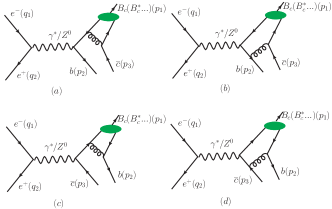
Figure 1: Feynman diagrams for the process $e^{-}(q_{1})+e^{+}(q_{2})\rightarrow(c\bar{b})[n](p_{1})+b(p_{2})+\bar{c}(p_{3})$.

The diquark state $(c\bar{b})[n]$, being color-singlet only, is considered here. Moreover, the matrix element can directly relate to the S-wave wave function at origin for $B_{c}$ meson, and the derivative of the wave function at origin for its P-wave excited states etc under potential framework, and the wave function itself and its derivative at origin can be calculated via potential model pot1 ; pot2 ; pot3 ; pot4 ; pot5 ; pot6 .

It is easy to check that, of the Feynman diagrams FIG.1 responsible for the production, the first two (a) and (b) are gauge invariant, and the rest two (c) and (d) are also gauge invariant. Thus it makes sense to separate the contributions from (a) and (b), and from (c) and (d) accordingly. Furthermore, based on calculations of the contributions from all of the four diagrams, and the contributions from the two subgroup diagrams mentioned here, one may pick out the contribution from interference of the two subgroup. In fact, the fragmentation function from an anti-$b$-quark to $B_{c}$ meson or its excited states is extracted from the contributions of the subgroup diagrams (a) and (b), and the fragmentation function from an $c$-quark to $B_{c}$ meson or its excited states is extracted from the contributions of the subgroup diagrams (c) and (d).

According to NRQCD, the unpolarized differential cross section $d\hat{\sigma}(e^{+}+e^{-}\to(c\bar{b})[n]+b+\bar{c})$, which stands for the short-distance factor, may be written down straightforwardly

$$d\hat{\sigma}(e^{+}+e^{-}\to(c\bar{b})[n]+b+\bar{c})=\frac{\overline{\sum}|M|^{2}d\Phi_{3}}{4\sqrt{(q_{1}.q_{2})^{2}-m_{e}^{4}}},$$ (2)

where $\overline{\sum}$ means that the spins in the initial state are averaged over, and the spins and colors in final state are summed over. The three-body phase space for the final state can be represented as

$$d{\Phi_{3}}=(2\pi)^{4}\delta^{4}\left(q_{1}+q_{2}-\sum_{f=1}^{3}p_{f}\right)\prod_{f=1}^{3}\frac{d^{3}{p_{f}}}{(2\pi)^{3}2p_{f}^{0}}.$$

The scattering amplitude corresponding to each Feynman diagram for the process $e^{+}+e^{-}\rightarrow(c\bar{b})[n]+b+\bar{c}$ can be written as:

$$iM={\kappa}L_{rr^{\prime}}^{\mu}D_{\mu\nu}H_{ss^{\prime}}^{\nu},$$ (3)

where

$$L_{rr^{\prime}}^{\mu}={\bar{v}_{r}}({q_{2}})\Gamma^{\mu}{u_{r^{\prime}}}({q_{1}})$$ (4)

and

$$H_{ss^{\prime}}^{\nu}={\bar{u}_{s}}({p_{2}}){\cal A}^{\nu}{v_{s^{\prime}}}({p_{3}})\,.$$ (5)

For $Z^{0}$-boson propagation diagrams, here $\kappa=\frac{e^{2}g_{s}^{2}}{\sin^{2}\theta_{w}\cos^{2}\theta_{w}}{\cal{C}}_{ij}$, the color factor ${\cal{C}}_{ij}=\frac{4}{3\sqrt{3}}\delta_{ij}$ (for the diquark $(c\bar{b})[n]$ in color singlet), the vertex $\Gamma^{\mu}=\gamma^{\mu}(1-4\sin^{2}\theta_{w}-\gamma_{5})$ and $D_{\mu\nu}=\frac{i}{k^{2}-m_{z}^{2}+im_{z}\Gamma_{z}}(-g_{\mu\nu}+k_{\mu}k_{\nu}/k^{2})$. For photon propagation diagrams, $\kappa=Qe^{2}g_{s}^{2}{\cal{C}}_{ij}$, $\Gamma^{\mu}=\gamma^{\mu}$ and $D_{\mu\nu}=\frac{-ig_{\mu\nu}}{k^{2}}$, where Q denotes the electric charge of the heavy quark which couples to the virtual photon. ${\cal A}^{\nu}$, corresponding to the precise spin $S$ and orbit $L$ of the diquak state $(c\bar{b})[n]$, are follows:

$${\cal A}^{S=0,L=0} = {\cal T}|_{q=0},$$ (6)

$${\cal A}^{S=1,L=0} = \varepsilon_{\beta}^{r}(p_{1}){\cal T}|_{q=0},$$ (7)

$${\cal A}^{S=0,L=1} = \varepsilon_{\alpha}^{l}(p_{1})\frac{d}{dq_{\alpha}}{\cal T}|_{q=0},$$ (8)

$${\cal A}^{S=1,L=1} = \varepsilon_{\alpha\beta}^{J}(p_{1})\frac{d}{dq_{\alpha}}{\cal T}|_{q=0},$$ (9)

where $\varepsilon_{\beta}^{r}(p_{1})$, $\varepsilon_{\beta}^{l}(p_{1})$ are the polar vectors relating to spin or orbit angular momentum in triplet for $(c\bar{b})[n]$-diquark, and $\varepsilon_{\alpha\beta}^{J}(p_{1})\,\;(J=0,1,2)$ is the polar tensor of the diquark in P-wave and spin-triplet states. ${\cal T}_{i}\,(i=1,2,3,4)$ relating to the Feynman diagrams accordingly in FIG.1 are as follows:

$${\cal T}_{1} = {{\gamma^{\nu}}{\Gamma_{b}}\frac{\not{p}_{2}-\not{k}+{m_{b}}}{(p_{2}-k)^{2}-m_{b}^{2}}{\gamma^{\rho}}\frac{\Pi_{p_{1}}(q)}{(p_{11}+{p_{3}})^{2}}{\gamma_{\rho}}},$$ (10)

$${\cal T}_{2} = {{\gamma^{\rho}}\frac{\not{k}-\not{p}_{12}+{m_{b}}}{(k-p_{12})^{2}-m_{b}^{2}}{\gamma^{\nu}}{\Gamma_{b}}\frac{\Pi_{p_{1}}(q)}{(p_{11}+{p_{3}})^{2}}{\gamma_{\rho}}},$$ (11)

$${\cal T}_{3} = {{\gamma^{\rho}}\frac{\Pi_{p_{1}}(q)}{(p_{12}+{p_{2}})^{2}}{\gamma_{\rho}}}\frac{\not{k}-\not{p}_{3}+{m_{c}}}{(k-p_{3})^{2}-m_{c}^{2}}{\gamma^{\nu}}{\Gamma_{c}},$$ (12)

$${\cal T}_{4} = {{\gamma^{\rho}}\frac{\Pi_{p_{1}}(q)}{(p_{12}+{p_{2}})^{2}}{\gamma^{\nu}}{\Gamma_{c}}\frac{\not{p}_{11}-\not{k}+{m_{c}}}{(p_{11}-k)^{2}-m_{c}^{2}}{\gamma_{\rho}}},$$ (13)

where $\Gamma_{c}=\frac{1}{4}-\frac{2}{3}\sin^{2}\theta_{w}-\frac{1}{4}\gamma^{5}$ for $Z-c\bar{c}$ vertex, and $\Gamma_{b}=-\frac{1}{4}+\frac{1}{3}\sin^{2}\theta_{w}+\frac{1}{4}\gamma^{5}$ for $Z-b\bar{b}$ vertex for $Z^{0}$ propagation diagrams, and $\Gamma_{b}=\Gamma_{c}=1$ for $\gamma-b\bar{b}$ and $\gamma-c\bar{c}$ vertex for photon propagation diagrams. $q$ is the relative momentum between the two quarks inside the $(c\bar{b})[n]$-diquark, and $p_{11}$, $p_{12}$ introduced here are the momenta of the two quarks inside the diquark $(c\bar{b})[n]$, i.e.

$$p_{11}=\frac{m_{c}}{M}p_{1}+q~{}~{}{\rm and}~{}~{}p_{12}=\frac{m_{b}}{M}p_{1}-q,$$ (14)

where $M\simeq m_{b}+m_{c}$ stands for the mass of $B_{c}$ meson or its excited states i.e. $(c\bar{b})[n]$ diquark. The projectors for spin singlet and triplet may be approximately written as follows:

$$\Pi^{0}_{p_{1}}(q)=\frac{-\sqrt{M}}{{4{m_{b}}{m_{c}}}}(\not{p}_{12}-m_{b})\gamma_{5}(\not{p}_{11}+m_{c}),$$ (15)

$$\Pi^{\beta}_{p_{1}}(q)=\frac{-\sqrt{M}}{{4{m_{b}}{m_{c}}}}(\not{p}_{12}-m_{b})\gamma^{\beta}(\not{p}_{11}+m_{c}).$$ (16)

After substituting these projectors into the above amplitudes, then we square the amplitudes, and sum over the final degrees of freedom. For appropriate total angular momentum, we also perform polarization summation properly. We define:

$$\Pi_{\alpha\beta}=-g_{\alpha\beta}+\frac{p_{1\alpha}{p_{2\beta}}}{M^{2}},$$ (17)

and the summation over the polarization for a spin triplet S-wave state or a spin singlet P-wave state is given by

$$\sum\limits_{J_{z}}\varepsilon_{\alpha}\varepsilon^{*}_{\alpha^{\prime}}=\Pi_{\alpha\alpha^{\prime}},$$ (18)

where $J_{z}$ can be $r_{z}$ or $l_{z}$ for spin and orbit projection respectively. As for the three multiplets ${}^{3}P_{J}$ with J=0, 1 and 2, the summation over the polarizations is given by

$$\varepsilon^{(0)}_{\alpha\beta}\varepsilon^{(0)*}_{\alpha^{\prime}\beta^{\prime}} = \frac{1}{3}\Pi_{\alpha\beta}\Pi_{\alpha^{\prime}\beta^{\prime}},$$ (19)

$$\sum_{J_{z}}\varepsilon^{(1)}_{\alpha\beta}\varepsilon^{(1)*}_{\alpha^{\prime}\beta^{\prime}} = \frac{1}{2}(\Pi_{\alpha\alpha^{\prime}}\Pi_{\beta\beta^{\prime}}-\Pi_{\alpha\beta^{\prime}}\Pi_{\alpha^{\prime}\beta}),$$ (20)

$$\sum_{J_{z}}\varepsilon^{(2)}_{\alpha\beta}\varepsilon^{(2)*}_{\alpha^{\prime}\beta^{\prime}} = \frac{1}{2}(\Pi_{\alpha\alpha^{\prime}}\Pi_{\beta\beta^{\prime}}+\Pi_{\alpha\beta^{\prime}}\Pi_{\alpha^{\prime}\beta})-\frac{1}{3}\Pi_{\alpha\beta}\Pi_{\alpha^{\prime}\beta^{\prime}}.$$

Since technically the colliding $e^{+}e^{-}$ beams for a $Z$-factory can be polarized, so it is interesting to consider the cases. To calculate the polarized cross sections for polarized electron and positron beams, we choose the the helicity states of the initial electron and positron to describe their polarization states, and we can use the projection operators

$$P_{L}=\frac{1-\gamma^{5}}{2},~{}~{}P_{R}=\frac{1+\gamma^{5}}{2},$$ (22)

to project out the polarized cross section. We note that in our calculations, the masses of electron and positron are ignored, so under the approximation and with a gauge boson photon or $Z$ boson mediating as shown in FIG.1, only two polarization cases, $e_{R}^{+}e_{L}^{-}$ and $e_{L}^{+}e_{R}^{-}$, contributes to the production. Thus now the polarized cross sections can be obtained by means of substituting Eq.(4) with

$${\bar{v}_{r}}({q_{2}})\Gamma^{\mu}P_{L}{u_{r^{\prime}}}({q_{1}}),$$ (23)

and

$${\bar{v}_{r}}({q_{2}})\Gamma^{\mu}P_{R}{u_{r^{\prime}}}({q_{1}}),$$ (24)

for $e_{R}^{+}e_{L}^{-}$ and $e_{L}^{+}e_{R}^{-}$, respectively.

Putting on the nonperturbative matrix element $\langle{\cal O}^{H}(n)\rangle$ ($H\equiv B_{c}$) accordingly as that in Eq.(II.1), the cross sections for $B_{c}$-meson production are obtained by integrating over the final phase space. For the production of excited states, the cross sections can be obtained similarly, as long as $[n]$ in $(c\bar{b})[n]$ and $H$ in $\langle{\cal O}^{H}(n)\rangle$ are matched properly.

II.2 The fragmentation functions and production under the fragmentation approach

The fragmentation approach for the production is based on the perturbative QCD factorization theorem: to calculate the relevant quark-pair production processes $e^{+}+e^{-}\rightarrow b+\bar{b}$ and $e^{+}+e^{-}\rightarrow c+\bar{c}$ respectively first and then to apply the fragmentation functions for a $\bar{b}$-quark to $B_{c}$ meson and for a $c$-quark to $B_{c}$ meson accordingly to the quark-pair production processes at the factorization energy scale $\mu$ properly. Here, more precisely, the fragmentation functions for the production are extracted from a relevant process under QCD complete calculations as the above, then need further to do evolution of them to the factorization energy scale $\mu$.

Namely the inclusive differential cross section can be written as:

$$\displaystyle\frac{d\sigma(z,\mu)}{dz}=\sum_{i}\int_{z}^{1}\frac{dy}{y}\times$$

$$\displaystyle\frac{d\sigma(e^{+}+e^{-}\to i(y)+X,\mu)}{dy}D_{i\to B_{c}}(z/y,\mu)\,,$$ (25)

where the $i$ represents the mediate partons, i.e. $c$-quark or $\bar{b}$-quark, and $z$ represents the energy fraction of the $B_{c}$-meson from $i$-quark, here it can be defined as

$$z=\frac{2k\cdot p_{1}}{k^{2}},$$ (26)

and $k$ is the four-momentum of the $Z$-boson or the photon, $\mu$ is the factorization energy-scale. Up-to LO and at the energy scale $\mu\simeq m_{{}_{Z}}$, the factorization formula reads

$$\frac{d\sigma}{dz}=\sum_{i}\sigma^{LO}(e^{+}+e^{-}\rightarrow i+\bar{i})D_{i\to B_{c}(B^{*}_{c},\cdots)}(z,\mu),$$ (27)

here the mediate parton $i$ can be either $c$-quark or $\bar{b}$-quark. Note that all the large logarithm terms $ln(m_{{}_{Z}}^{2}/\mu^{2})$, which come from the collinear emissions for high order calculations, also disappear due to the factorization energy scale $\mu$ being set to $m_{{}_{Z}}$.

The strategy for the fragmentation approach is firstly to extract the fragmentation functions from the process $e^{-}+e^{+}\to b+\bar{c}+B_{c}(B^{*}_{c},\cdots)$ near the threshold $k^{2}=4(m_{c}+m_{b})^{2}$ i.e. the fragmentation functions $D_{\bar{b}\to B_{c}(B^{*}_{c},\cdots)}(z,\mu_{0})$ with $\mu_{0}\simeq m_{b}+2m_{c}$ and $D_{c\to B_{c}(B^{*}_{c},\cdots)}(z,\mu_{0})$ with $\mu_{0}\simeq m_{c}+2m_{b}$ are obtained by the extraction, then to do evolution on them to the fragmentation energy scale $\mu=m_{{}_{Z}}$, and finally the production we are interested in here is computed out in terms of Eq.(27). Now let us show how to extract the fragmentation functions from the perturbative calculations and then to do the evolution to the factorization energy scale $\mu=m_{{}_{Z}}$ for application here.

Precisely we only describe the way for extracting the fragmentation function of $B_{c}$-meson, because extracting the fragmentation functions of the excited states is similar, as long as the different quantum numbers of the diquark $(c\bar{b})[n]$ and different matrix element $\langle{\cal O}^{H}(n)\rangle$ are taken into account.

For convenience, we define some kinematic variables as follows:

$$x=\frac{2k\cdot p_{2}}{k^{2}},\,y=\frac{2k\cdot p_{3}}{k^{2}},\,d=\frac{M^{2}}{k^{2}},\,r_{1}=\frac{m_{c}}{M},\,r_{2}=\frac{m_{b}}{M}\,,$$ (28)

here $M=m_{{}_{B_{c}}}$ when $B_{c}$ fragmentation function is concerned, and $k$ is the momentum of the virtual photon or $Z$-boson in FIG.1.

To extract $D_{\bar{b}\to B_{c}}(z,\mu_{0})$, the differential cross sections and total cross sections of the production $e^{+}+e^{-}\to b+\bar{c}+B_{c}$ at $k^{2}\geq 4(m_{c}+m_{b})^{2}$ via $\bar{b}$-quark production by mediating virtual photon (here $k^{2}$ is much smaller than $m^{2}_{Z}$, so the contributions from $Z$-boson mediation can be ignored) i.e. of diagrams (a) and (b) in FIG.1 only those via virtual photon are needed to be computed precisely. Namely the fragmentation functions $D_{\bar{b}\to B_{c}}(z,\mu_{0})$ with $\mu_{0}\simeq m_{b}+2m_{c}$ is extracted with the process $e^{+}+e^{-}\to b+\bar{c}+B_{c}$ just at the threshold (above a little) as

$$D_{\bar{b}\to B_{c}}(z,\mu_{0})=\frac{1}{\sigma^{LO}(e^{+}e^{-}\to b\bar{b})}\frac{d\sigma(e^{+}e^{-}\to\bar{b}\to B_{c})}{dz}\,.$$ (29)

If $d\ll 1$, the double differential cross section of S-wave states can be written approximately as

$$\displaystyle\frac{1}{\sigma_{0}}\frac{d^{2}\sigma}{dx~{}dz} \displaystyle\simeq\frac{8\alpha_{s}^{2}(4m^{2}_{c})|\Psi_{S}(0)|^{2}}{27k^{2}Mr_{1}^{2}(1-r_{2}z)^{2}}\displaystyle\left[\frac{w_{0}(z)}{(1-x)^{2}}+\frac{d~{}w_{1}(z)}{(1-x)^{3}}+\frac{d^{2}~{}w_{2}(z)}{(1-x)^{4}}\right]\,,$$ (30)

here $\sigma_{0}=\sigma^{LO}(e^{+}+e^{-}\rightarrow b+\bar{b})$. As pointed out by the authors of Ref.zbc1 , owing to $d\ll 1$, the terms with positive and larger than -2 power of (1-x) may be ignored, but when x being integrated, a factor $1/d$ is obtained form each $1/(1-x)$ factor, so the terms containing $w_{0}(z)$, $w_{1}(z)$ and $w_{2}(z)$ in Eq.(30) should be kept. The integral bounds of x at a fixed z now can be written as

$$(1-x)_{min}\simeq\frac{(1-r_{2}z)^{2}d}{z(1-z)}\,,\;\;\;(1-x)_{max}\simeq z-\frac{(1-r_{1}z)^{2}d}{z(1-z)}\,,$$ (31)

and the integral over the range of $x$ is performed, so the fragmentation functions are obtained:

$$D_{\bar{b}\to B_{c}(B_{c}^{*})}(z,\mu_{0})=\frac{8\alpha_{s}^{2}(4m^{2}_{c})|\Psi_{S}(0)|^{2}}{27m_{c}^{2}M(1-r_{2}z)^{2}}\left[\delta w_{0}(z)+\frac{\delta^{2}}{2}w_{1}(z)+\frac{\delta^{3}}{3}w_{2}(z)\right]\,,$$ (32)

where $\delta=\frac{z(1-z)}{(1-r_{2}z)^{2}}$. When the fragmentation functions for P-wave states $B_{c,J(P)}^{*}$, i.e. $(\bar{b}c)$ in P-wave states, are extracted, the relevant double differential cross sections are replaced as

$$\frac{1}{\sigma_{0}}\frac{d^{2}\sigma}{dx~{}dz}=\frac{128\alpha_{s}^{2}(4m^{2}_{c})|\Psi^{\prime}_{P}(0)|^{2}}{27k^{2}M^{3}r_{1}^{4}(1-r_{2}z)^{4}}\left[\frac{w_{0}(z)}{(1-x)^{2}}+\frac{d~{}w_{1}(z)}{(1-x)^{3}}+\frac{d^{2}~{}w_{2}(z)}{(1-x)^{4}}+\frac{d^{3}~{}w_{3}(z)}{(1-x)^{5}}+\frac{d^{4}~{}w_{4}(z)}{(1-x)^{5}}\right],$$ (33)

where the coefficients $w_{0}(z)$, $w_{1}(z)$, $w_{2}(z)$, $w_{3}(z)$ and $w_{4}(z)$ for P-wave states can be computedzbc1 ; fragbc1 ; fragbc2 . Integrating the double differential cross sections over variable $x$, we obtain

$$\displaystyle D_{\bar{b}\to B_{c,J(P)}^{*}}(z,\mu_{0})=\frac{128\alpha_{s}^{2}(4m^{2}_{c})|\Psi^{\prime}_{P}(0)|^{2}}{27m_{c}^{4}M(1-r_{2}z)^{4}} \left[\delta w_{0}(z)+\frac{\delta^{2}}{2}w_{1}(z)+\frac{\delta^{3}}{3}w_{2}(z)+\frac{\delta^{4}}{4}w_{3}(z)+\frac{\delta^{5}}{5}w_{4}(z)\right].$$ (34)

For extracting the fragmentation functions $D_{c\to B_{c}(B^{*}_{c},\cdots)}(z,\mu_{0})$, the way is similar but the diagrams (c) and (d) instead of the diagrams (a) and (b) in FIG.1 are computed. One may also find that by interchanging $r_{1}\leftrightarrow r_{2}$ and $\alpha_{s}^{2}(4m^{2}_{c})$, $\mu_{0}=2m_{c}+m_{b}$ being replaced by $\alpha_{s}^{2}(4m^{2}_{b})$, $\mu_{0}=m_{c}+2m_{b}$ respectively, so the fragmentation functions $D_{c\to B_{c}(B^{*}_{c},\cdots)}(z,\mu_{0})$ may be obtained in terms of the interchanges from the one $D_{\bar{b}\to B_{c}(B^{*}_{c},\cdots)}(z,\mu_{0})$ as pointed.

Having the fragmentation functions, we need to do the needed evolution from $\mu_{0}$ to the energy scale $\mu=m_{{}_{Z}}$, where the factorization is made for the concerned production.

The evolution of the fragmentation functions are governed by the DGLAP equation AP ,

$$\mu\frac{\partial}{\partial\mu}D_{i\to B_{c}(B^{*}_{c},\cdots)}(z,\mu)$$ (35)

$$= \frac{\alpha_{s}(\mu)}{\pi}\sum_{j}\int^{1}_{z}\frac{dy}{y}P_{i\to j}(z/y)D_{j\to B_{c}(B^{*}_{c},\cdots)}(y,\mu),$$

where $i$ and $j$ are all possible partons, but here $j=i$. For $B_{c}(B^{*}_{c},\cdots)$-meson production, $i$ can be $c$-quark or $\bar{b}$-quark, and

$$P_{i\to i}(z)=\frac{4}{3}\left(\frac{1+z^{2}}{1-z}\right)_{+},$$ (36)

is the splitting function. Using the approximate method to solve the DGLAP equation APsolve , we obtain

$$D_{i\to B_{c}(B^{*}_{c},\cdots)}(z,\mu)=R\otimes D_{i\to B_{c}(B^{*}_{c},\cdots)}(z,\mu_{0})$$

$$+\kappa R\otimes P_{\Delta}\otimes D_{i\to B_{c}(B^{*}_{c},\cdots)}(z,\mu_{0}),$$ (37)

where $\kappa=\frac{2}{\beta_{0}}{\rm ln}\left(\frac{\alpha_{s}(\mu_{0}^{2})}{\alpha_{s}(\mu^{2})}\right)$, it is not the coefficient $\kappa$ we defined in the amplitudes in Sec.II.1, $\otimes$ is the convolution which is defined as

$$A\otimes B=\int^{1}_{z}\frac{dy}{y}A(z/y)B(y),$$ (38)

and

$$R(z)=\frac{\left(-{\rm ln}(z)\right)^{8\kappa/3-1}}{\Gamma(8\kappa/3)},$$ (39)

and

$$P_{\Delta}(y)=\frac{4}{3}\left[\frac{1+y^{2}}{1-y}+\frac{2}{{\rm ln}(y)}+(\frac{3}{2}-2\gamma_{E})\delta(1-y)\right].$$ (40)

Thus the fragmentation functions are evolved to the energy scale of $m_{{}_{Z}}$ with the formulas.

II.3 The production of doubly heavy baryons

In this subsection we consider the production of the doubly heavy baryons $(QQ^{\prime}q)$, where $Q$ and $Q^{\prime}$ mean heavy quarks $c$ and/or $b$ but $q$ means light quark.

The approach, which we adopt here, for the production is to divide it into two steps. The first step is that a binding diquark $<QQ^{\prime}>$ ($Q$ and $Q^{\prime}$ may $b$-quark or $c$-quark) with ‘suitable’ quantum numbers is produced, precisely $<QQ^{\prime}>$ may be in color anti-triplet or sextuplet, and the second step is that the diquark ’fragments’ to a doubly heavy baryon $(QQ^{\prime}q)$ through caching a light quark from ’environment’ with a fragmentation probability of almost one hundred percent, i.e. it is implied that the produced doubly heavy diquark always makes a doubly heavy baryon accordingly. Here for the first step, we compute the production of doubly heavy diquarks under the QCD complete approach similar to that of $B_{c}$ meson but the matrix element $\langle{\cal O}^{B_{c}}(n)\rangle$ should be replaced by a proper one $\langle{\cal O}^{<QQ^{\prime}>}(n)\rangle$. Namely

$$d\sigma(e^{+}+e^{-}\to<QQ^{\prime}>+\bar{Q}+\bar{Q^{\prime}})=$$

$$\sum_{n}d\hat{\sigma}(e^{+}+e^{-}\to(QQ^{\prime})[n]+\bar{Q}+\bar{Q^{\prime}})\times$$

$$\langle{\cal O}^{<QQ^{\prime}>)}(n)\rangle\,.$$ (41)

We should note here that the energy scale in fragmentation approach is $2m_{Q}+m_{Q^{\prime}}$ or $m_{Q}+2m_{Q^{\prime}}$ similar to the case of $B_{c}$ meson.

For the production of $<bc>$-diquark, there are four Feynman diagrams responsible for it, which are the same as that of $B_{c}$ meson production showed in FIG.1 except the fermion line of the b-quark being reversed. For the production of $<cc>$-diquark and $<bb>$-diquark, besides the four diagrams corresponding to those showed in FIG.1, there are more four diagrams obtained by an interchange of two quark lines of the diquark.

In order to calculate the amplitude of the diquark production, we adopt the method used in Refs.eeXi ; doublybaryon3 . We reverse one of the fermion lines of the heavy quark through charge conjugate transformation firstly, and then similarly to writing down the amplitude of doubly heavy meson production showed above, we directly write down the requested amplitude for the binding diquark production. Precisely a fermion line appearing in diquark production can be written as,

$$Am=\bar{u}_{s_{1}}\left(\frac{m_{Q}}{M}p_{1}\right)\Gamma_{n}s_{f}(k_{n-1},m_{Q})\times$$

$$\cdots s_{f}(k_{1},m_{Q})\Gamma_{1}v_{s_{2}}(p_{2}),$$ (42)

where $s_{f}(k_{i},m_{Q})$ is the fermion propagator, $\Gamma_{i}$ is the interaction vertex, $m_{Q}$ is heavy quark mass of the fermion line, and $n$ is the number of the interaction vertices. Using the charge conjugation matrix $C=-i\gamma^{2}\gamma^{0}$, we can obtain the following transformation,

$$v^{T}_{s_{2}}(p_{2})C=-\bar{u}_{s_{2}}(p_{2}),C^{-}\bar{u}_{s_{1}}\left(\frac{m_{Q}}{M}p_{1}\right)^{T}=v_{s_{1}}\left(\frac{m_{Q}}{M}p_{1}\right),$$

$$C^{-}(\gamma^{\alpha})^{T}C=-\gamma^{\alpha},~{}~{}~{}~{}C^{-}(\gamma^{\alpha}\gamma^{5})^{T}C=\gamma^{\alpha}\gamma^{5}$$

$$C^{-}s_{f}^{T}(-k_{i},m_{Q})C=s_{f}(k_{i},m_{Q})\,.$$ (43)

If the fermion line contains no axial vector vertex, we have

$$Am^{T} = v_{s_{2}}^{T}(p_{2})\Gamma_{1}^{T}s_{f}^{T}(k_{1},m_{Q})\cdots s_{f}^{T}(k_{n-1},m_{Q})\Gamma_{n}^{T}\bar{u}_{s_{1}}\left(\frac{m_{Q}}{M}p_{1}\right)^{T}$$ (44)

$$= v_{s_{2}}^{T}(p_{2})CC^{-}\Gamma_{1}^{T}CC^{-}s_{f}^{T}(k_{1},m_{Q})C\cdots C^{-}s_{f}^{T}(k_{n-1},m_{Q})CC^{-}\Gamma_{n}^{T}CC^{-}\bar{u}_{s_{1}}\left(\frac{m_{Q}}{M}p_{1}\right)^{T}$$

$$= (-1)^{(n+1)}\bar{u}_{s_{2}}(p_{2})\Gamma_{1}s_{f}(-k_{1},m_{Q})\cdots s_{f}(-k_{n-1},m_{Q})\Gamma_{n}v_{s_{1}}\left(\frac{m_{Q}}{M}p_{1}\right)\,.$$

If the fermion line contains an axial vector vertex, then a (-1) factor should be contained. After reversing the heavy qaurk line, we can transform the amplitude of the diquark production to meson production except an additional $(-1)^{(n+1)}$ factor for pure vector case ($(-1)^{(n+2)}$ factor for containing an axial vector case). i.e. the amplitude of $(bc)[n]$-diquark production can be represented as

$$M_{diquark}=(M^{a}_{1}-M^{v}_{1})+(M^{a}_{2}-M^{v}_{2})+M_{3}+M_{4},$$ (45)

where $M_{1},M_{2},M_{3},M_{4}$ are the amplitude of $B_{c}$ production showed above, and $M^{a}_{i}$,$M^{v}_{i}$ are those for the cases containing an axial vector or pure vector cases of $M_{i}$ respectively. As we have mentioned above, for the $<cc>$-diquark and $<bb>$-diquark productions there are four more diagrams come from the exchange of the two identical quark line inside the diquark. Since the relative velocity between the two quarks inside the diquark, $v$, is set to be zero up-to the lowest order non-relativistic approximation, the contributions from additional diagrams are the same as the four diagrams relating to heavy quarkonium production. There is one (1/2!) factor comes from wave function of identical particles in diquark. Thus we only need to calculate the four diagrams, and multiplying the cross section by $(2^{2}/2!)=2$.

According to the decomposition $\textbf{3}\otimes\textbf{3}=\bar{\textbf{3}}\oplus\textbf{6}$, $(bc)[n]$-diquark can be in $\bar{\textbf{3}}$ or 6 color state. It is known that ‘one-gluon exchange’ interaction is important inside the diquark, and the interaction inside the diquark in $\bar{\textbf{3}}$ state is attractive, but that in 6 state is repulsive, so people believe that the ’binding force’ (including the confinement interaction besides one-gluon exchange) in $\bar{\textbf{3}}$ is stronger than that in 6, i.e. we have the consequence $\langle{\cal O}^{<QQ^{\prime}>}\rangle\,_{\bar{\textbf{3}}}>\langle{\cal O}^{<QQ^{\prime}>}\rangle\,_{\textbf{6}}$, hence in this paper we will ignore the contributions from the color 6 component. According to the request of Fermi-Dirac statistics for quarks, the wave functions of the diquark should be totally antisymmetric under exchange of the two quarks inside the diquarks, so for the production of the ground state of the diquaks, $<bb>$ and $<cc>$, which is concerned here only, the diquark wave function should be S-wave and in color anti-triplet and spin triplet.

The color factor for color anti-triplet diquark production can be represented as follows:

$${\cal{C}}_{ij}={\cal{N}}\sum_{a}\sum_{m,n}T^{a}_{im}T^{a}_{jn}\varepsilon_{mnk},$$ (46)

where ${\cal{N}}=1/\sqrt{2}$ is the normalization constant, $\varepsilon_{mnk}$ is the the antisymmetric tensor for the $\bar{\textbf{3}}$ state and it is satiesfy $\varepsilon_{mnk}\varepsilon_{m^{\prime}n^{\prime}k}=\delta_{mm^{\prime}}\delta_{nn^{\prime}}-\delta_{mn^{\prime}}\delta_{nm^{\prime}}$. After squaring we obtain that ${\cal{C}}^{2}_{ij}=4/3$ for the $\bar{\textbf{3}}$ state.

III Numerical Results

III.1 The production of $B_{c}(B^{*}_{c},\cdots)$-mesons

When doing the numerical calculations under complete QCD approach and fragmentation approach, the input parameters are taken as follows:

$$m_{b}=4.9~{}{\rm GeV},m_{c}=1.5~{}{\rm GeV},m_{Z}=91.1876~{}{\rm GeV},$$

$$\sin^{2}\theta_{w}=0.231,\alpha=1/128,|R_{S}(0)|^{2}=1.642~{}{\rm GeV^{3}},$$

$$|R^{\prime}_{P}(0)|^{2}=0.201~{}{\rm GeV^{5}},$$ (47)

where $\alpha=\alpha(m^{2}_{{}_{Z}})$ is the electromagnetic coupling constant; $R_{S}(0)$ and $R^{\prime}_{P}(0)$ are the ridial wave function of the ($B_{c}(B^{*}_{c},\cdots)$) and its derivative of the relevant states at origion respectively and taken from potential model pot6 .

As for the strong coupling constant, we take $\alpha_{s}(m^{2}_{Z})=0.1185$ PDG as the reference point, and by one loop running coupling we obtain the request values $\alpha_{s}(4m^{2}_{c})=0.237$ and $\alpha_{s}(4m^{2}_{b})=0.175$.

contribution	total	$\bar{b}$-frag.	$c$-frag.	interference
$\sigma(B_{c},\;^{1}S_{0})$	2.734	2.613	5.20$\times 10^{-2}$	6.90$\times 10^{-2}$
$\sigma(B^{*}_{c},\;^{3}S_{1})$	3.823	3.722	4.45$\times 10^{-2}$	5.65$\times 10^{-2}$
$\sigma(B^{**}_{c},\;^{1}P_{1})$	0.271	0.269	3.01$\times 10^{-3}$	-1.01$\times 10^{-3}$
$\sigma(B^{**}_{c},\;^{3}P_{0})$	0.164	0.157	8.13$\times 10^{-3}$	-1.13$\times 10^{-3}$
$\sigma(B^{**}_{c},\;^{3}P_{1})$	0.340	0.331	5.77$\times 10^{-3}$	3.23$\times 10^{-3}$
$\sigma(B^{**}_{c},\;^{3}P_{2})$	0.365	0.366	3.87$\times 10^{-4}$	-1.39$\times 10^{-3}$

Table 1: The cross section (in $pb$) of $e^{-}e^{+}\to B_{c}(B^{*}_{c},\cdots)+b+\bar{c}$ at $Z$-pole under complete QCD calculation. $\bar{b}$-frag., $c$-frag. and ’Interferance’ denote the contributions from the first two diagrams in FIG.1, those from the last two diagrams in FIG.1 and those from the interference of the first two diagrams and the last two diagrams in FIG.1.

The two diagrams (a), (b) and the other two diagrams (c), (d) as well of FIG.1 are gauge invariant, thus in complete QCD calculation approach to separate the contributions from diagrams (a), (b) and those from diagrams (c), (d) as well as those from their ’interference’ makes sense. Especially note that in fragmentation approach the fragmentation from $\bar{b}$-quark takes into account the contribution from diagrams (a), (b) and the fragmentation from $c$-quark takes into account the contribution from diagrams (c), (d) respectively, whereas the interference contributions cannot be taken into account.

The numerical results of the cross sections at $Z$-pole under the QCD cmplete calculation with separation of the contributions: from (a), (b) diagrams ($\bar{b}$-frag.), from (c), (d) diagrams ($c$-frag.) and from interference are put in TABLE.1 .

contribution	total	$\bar{b}$-frag.	$c$-frag.
$\sigma(B_{c},\;^{1}S_{0})$	2.850	2.792	5.88$\times 10^{-2}$
$\sigma(B^{*}_{c},\;^{3}S_{1})$	3.974	3.923	5.08$\times 10^{-2}$
$\sigma(B^{**}_{c},\;^{1}P_{1})$	0.295	0.292	3.53$\times 10^{-3}$
$\sigma(B^{**}_{c},\;^{3}P_{0})$	0.170	0.160	9.08$\times 10^{-3}$
$\sigma(B^{**}_{c},\;^{3}P_{1})$	0.360	0.354	6.59$\times 10^{-3}$
$\sigma(B^{**}_{c},\;^{3}P_{2})$	0.396	0.395	4.74$\times 10^{-4}$

Table 2: The cross section (in $pb$) of $e^{-}e^{+}\to B_{c}(B^{*}_{c},\cdots)+\cdots$ at the $Z$-pole under fragmentation approach.

For comparison between the complete QCD approach (LO) and the fragmentation approach (LL), the results under the fragmentation approach are put in TABLE.2, where the contributions from $\bar{b}$-quark fragmentation and $c$-quark fragmentation are showed explicitly. One may see that the results for total cross-sections obtained from the two approaches are consistent each other. This is because that the property $\int_{0}^{1}dzP_{i\to i}(z)=0$ leads to non-evolution with $\mu$ for $\int_{0}^{1}dzD_{i\to B_{c}(B^{*}_{c},\cdots)}(z,\mu)$fragbc1 , so the total cross sections are same as the ones at the initial scale. It is easy to see that the fragmentation contributions dominantly come from the $\bar{b}$-quark fragmentation, i.e. the contributions from diagrams (a) and (b) in FIG.1 under the complete QCD calculation. The contributions from $c$-quark fragmentation are comparatively small and it is due to deeper depress from the gluon propagator in diagrams (c) and (d) than from that in diagrams (a) and (b).

The collision energy of initial $e^{+}e^{-}$ may not exactly at $Z$-pole, so we also show the behave of the cross sections around the $Z$-pole. We present the cross sections at several collison energies around the $Z$-pole in TABLE.3, and from it one can see that the cross sections decrease rapidly when the collision energy deviate from $m_{Z}$. When the collision energy deviate from $m_{Z}$ by $5$ GeV, i.e. about twice width of the $Z^{0}$ boson, the cross sections depressed by about one order, thus when studying $B_{c}$ and its excited states, sometimes it is crucial to make use of the effects of $Z^{0}$ resonance at an $e^{+}e^{-}$ collider.

$(\sqrt{s}-m_{{}_{Z}})$(GeV)	-5	-2.5	-1.5	-0.8	-0.4	-0.2	0	0.2	0.4	0.8	1.5	2.5	5
$\sigma(B_{c},\;^{1}S_{0})$	0.15	0.53	1.09	1.91	2.46	2.65	2.73	2.68	2.50	1.97	1.15	0.56	0.17
$\sigma(B^{*}_{c},\;^{3}S_{1})$	0.21	0.74	1.52	2.67	3.44	3.71	3.82	3.74	3.50	2.75	1.60	0.79	0.24
$\sigma(B^{**}_{c},\;^{1}P_{1})$	0.01	0.05	0.11	0.19	0.24	0.26	0.27	0.27	0.25	0.19	0.11	0.06	0.02
$\sigma(B^{**}_{c},\;^{3}P_{0})$	0.01	0.03	0.07	0.11	0.15	0.16	0.16	0.16	0.15	0.12	0.07	0.03	0.01
$\sigma(B^{**}_{c},\;^{3}P_{1})$	0.02	0.07	0.14	0.24	0.31	0.33	0.34	0.33	0.31	0.24	0.14	0.07	0.02
$\sigma(B^{**}_{c},\;^{3}P_{2})$	0.02	0.07	0.15	0.25	0.33	0.35	0.37	0.36	0.33	0.26	0.15	0.08	0.02

Table 3: The cross section (in $pb$) of $e^{-}e^{+}\to B_{c}(B^{*}_{c},\cdots)+b+\bar{c}$ varies with the collision energy around $m_{{}_{Z}}$ under complete QCD approach.

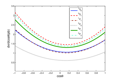
Figure 2: The differential cross sections $d\sigma/d\cos{\theta}$ for the production $e^{+}e^{-}\to B_{c}(B^{*}_{c},\cdots)+b+\bar{c}$ under complete QCD approach. In order to put all the results into the figure, the results of P-wave meson production are multiplied by a factor ten.

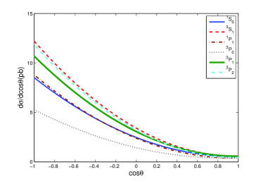
Figure 3: The differential cross sections $d\sigma/d\cos{\theta}$ for the production $e_{R}^{+}e_{L}^{-}\to B_{c}(B^{*}_{c},\cdots)+b+\bar{c}$ (with polarized incoming beams) under complete QCD approach. In order to put all the results into the figure the results for P-wave states are multiplied by a factor ten.

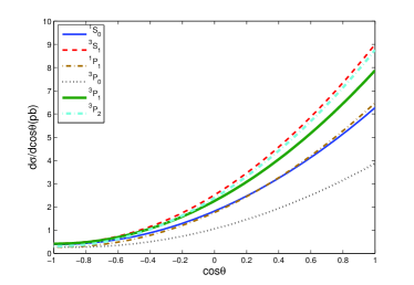
Figure 4: The differential cross sections $d\sigma/d\cos{\theta}$ for the production $e_{L}^{+}e_{R}^{-}\to B_{c}(B^{*}_{c},\cdots)+b+\bar{c}$ (with polarized incoming beams) under complete QCD approach. In order to put all the results into the figure the results for P-wave states are multiplied by a factor ten.

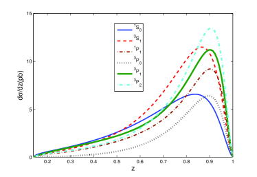
Figure 5: The differential cross sections $d\sigma/dz$ for the processes $e^{+}e^{-}\to B_{c}(B^{*}_{c},\cdots)+b+\bar{c}$ by complete QCD approach, where $z$ is the energy fraction carried by the concerned meson. The results for P-wave states are multiplied by a factor ten.

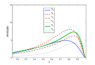
Figure 6: The differential cross sections $d\sigma/dz$ for the processes $e^{+}e^{-}\to B_{c}(B^{*}_{c},\cdots)+\cdots$ by $\bar{b}$-quark fragmentation under fragmentation approach, where $z$ is the energy fraction carried by the concerned meson. The results for P-wave states are multiplied by a factor ten.

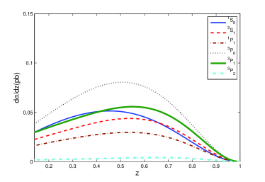
Figure 7: The differential cross sections $d\sigma/dz$ for the processes $e^{+}e^{-}\to B_{c}(B^{*}_{c},\cdots)+\cdots$ by $c$-quark fragmentation under fragmentation approach, where $z$ is the energy fraction carried by the concerned meson. The results for P-wave states are multiplied by a factor ten.

In order to know the characteristic of the production for experimental studying the mesons, we reserve the numerical results for the differential cross sections $d\sigma/d\cos{\theta}$ where $\theta$ is the angle between the momenta of the meson in final state and the electron in initial state under complete QCD approach, and present them in FIG.2.

From FIG.2, one may see clearly that the production has maximum near the collision axis. The differential cross sections also show us certain backward-forward asymmetry in the direction of the initial positron. It is caused by parity-violation in the interaction mediated by $Z^{0}$ boson exchange.

Since the incoming beams for the production may be polarized, so we also compute and present the angle distributions for polarized electron and and polarized positron beams in FIGs.3,4. But note that just for convenience, here we take helicities to take into account the polarizations. One may see the difference in magnitude between $Z^{0}$ boson coupling to left-handed helicity and right-handed helicity electron, and this leads the backward-forward asymmetry in FIG.2.

In FIG.5, we present the energy fractions ($z$ dependence) of $B_{c}(B^{*}_{c},\cdots)$ meson obtained by complete QCD approach (LO). The results are obtained by $\bar{b}$-quark fragmentation and by $c$-quark fragmentation under fragmentation approach are presented in FIG.6 and in FIG.7. Here for the fragmentation approach, we have evolved the scale of the fragmentation functions to $m_{Z}$. From the figures one may see that the contributions from $c$-quark fragmentation are smaller than those from $\bar{b}$-quark fragmentation by two magnitude orders, thus the $c$-quark fragmentation contributions in the production can be ignored. From FIGs.5,6 one may see that the production of $B_{c}(B^{*}_{c},\cdots)$ meson at low energy fraction (small $z$) estimated by the fragmentation approach is greater than that by complete QCD approach. Namely from the figures, one can see the differences from each other in distributions by the approaches clearly.

$\sqrt{s}$(GeV)	180	240
$\sigma(B_{c},\;^{1}S_{0})$	1.05	0.47
$\sigma(B^{*}_{c},\;^{3}S_{1})$	1.55	0.72
$\sigma(B^{**}_{c},\;^{1}P_{1})$	0.11	0.05
$\sigma(B^{**}_{c},\;^{3}P_{0})$	0.07	0.03
$\sigma(B^{**}_{c},\;^{3}P_{1})$	0.14	0.07
$\sigma(B^{**}_{c},\;^{3}P_{2})$	0.15	0.07

Table 4: The cross sections (in $fb$) of the production $e^{-}e^{+}\to B_{c}(B^{*}_{c},\cdots)+b+\bar{c}$ at 180 GeV and 240 GeV under complete QCD approach.

An $e^{+}+e^{-}$ collider running at energies 180 GeV and 240 GeV (above the threshold of WW and/or ZH production respectively) is very suitable for studying the properties of W-boson and Higgs boson etc, so to see the possibility for experimental studying $B_{c}(B^{*}_{c},\cdots)$ mesons at the collider at the same time is interesting. Therefore, we also estimate the meson production at the high energies for an $e^{+}+e^{-}$ collider, and put the results in TABLE.4. The results show that the cross sections are in $fb$, less than the cross sections at the $Z$-pole by $3\sim 4$ order, that means it is hopeless for studying $B_{c}(B^{*}_{c},\cdots)$ meson at such an $e^{+}+e^{-}$ collider running at the high energies even having so high luminosity as $\sim 10^{36}cm^{-2}s^{-1}$.

III.2 The production of doubly heavy baryons

To do the numerical calculations on the production of doubly heavy baryons, we adopt the parameters as follows,

$$m_{b}=5.1~{}{\rm GeV}\,,\;\;m_{c}=1.8~{}{\rm GeV}\,,$$

$$|\Psi_{(cc)}(0)|^{2}=0.039~{}{\rm GeV^{3}}\,,\;\;|\Psi_{(bc)}(0)|^{2}=0.065~{}{\rm GeV^{3}},$$

$$|\Psi_{(bb)}(0)|^{2}=0.152~{}{\rm GeV^{3}}\,,$$ (48)

which are the smae as Ref.doublybaryon4 . Note here that for the production of $\Xi_{cc}$ and $\Xi_{bc}$, the squared momentum transferred $Q^{2}$ carried by gluon is adopted as $4m^{2}_{c}$, whereas for the $\Xi_{bb}$, it is adopted as $4m^{2}_{b}$.

The cross sections of the diquark production obtained by our estimation:

$$\sigma_{|\left(cc\right){\scriptsize{}_{\overline{\textbf{3}}}}\,,^{3}S_{1}\rangle}=0.52~{}{\rm pb},~{}~{}\sigma_{|\left(bc\right){\scriptsize{}_{\overline{\textbf{3}}}}\,,^{1}S_{0}\rangle}=0.58~{}{\rm pb},$$

$$\sigma_{|\left(bc\right){\scriptsize{}_{\overline{\textbf{3}}}}\,,^{3}S_{1}\rangle}=0.79~{}{\rm pb},~{}~{}\sigma_{|\left(bb\right){\scriptsize{}_{\overline{\textbf{3}}}}\,,^{3}S_{1}\rangle}=0.04~{}{\rm pb}.$$

For the doubly heavy baryon production, we present the angle distributions (differential cross sections) in FIG.8 too, where the distributions for various channels are labeled precisely. One may see from the figure that the doubly heavy baryon production has certain backward-forward asymmetry too. However, the distributions are different from those of the $B_{c}$ meson production, namely the doubly heavy baryons are mainly concentrated in the direction of the initial electron. One can understand the reason by the fragmentation approach, that the mainly contribution of the $B_{c}$-meson production comes from the diagrams (a) and (b) in FIG.1, i.e. from the fragmentation of $\bar{b}$-quark. Since the produced $\bar{b}$-quark is concentrated in the direction of the initial positron around $Z$-pole, so there are more $B_{c}$ mesons along the direction of the initial positron. In contrast, the $\Xi_{cc}$ mainly from the fragmentation of c-quark, $\Xi_{bc}$ and $\Xi_{bb}$ from b-quark, where b-quarks and c-quarks are mainly along the direction of intial electron around $Z$-pole.

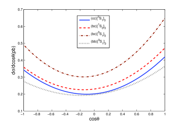
Figure 8: Differential cross sections $d\sigma/d\cos{\theta}$ for the production of the doubly heavy baryons under complete QCD approach, where $\theta$ is the angle between the momenta of the final baryon and the initial electron. In order to show in one figure, for $\Xi_{bb}$, it was multiplied by a factor ten.

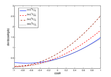
Figure 9: Angle distributions of the polarized differential cross sections $d\sigma/d\cos{\theta}$ for the production of the doubly heavy baryons with $e^{+}_{R}e^{-}_{L}$ polarization states under complete QCD approach, where $\theta$ is the angle between the momenta of the final baryon and the initial electron. In order to show in one figure, for $\Xi_{bb}$, it was multiplied by a factor ten.

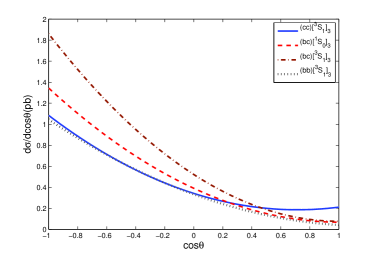
Figure 10: Angle distributions of the polarized differential cross sections $d\sigma/d\cos{\theta}$ for the production of the doubly heavy baryons with $e^{+}_{L}e^{-}_{R}$ polarization states under complete QCD approach, where $\theta$ is the angle between the momenta of the final baryon and the initial electron. In order to show in one figure, for $\Xi_{bb}$, it was multiplied by a factor ten.

As that above for $B_{c}$ meson production where the polarizations for incoming beams are considered, we also compute and present the angle distributions of $\Xi_{cc}$, $\Xi_{bc}$ and $\Xi_{bb}$ production in polarizations: $e^{+}_{R}e^{-}_{L}$ and $e^{+}_{L}e^{-}_{R}$ (in the other cases the results are zero) respectively in FIGs.9,10. From them, one can see the difference in magnitude for left-handed electron and right-handed electron easily, and it helps us understand the backward-forward asymmetry in the unpolarized differential cross sections.

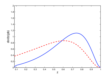
Figure 11: The differential cross sections $d\sigma/dz$ in $pb$ for the production of the doubly heavy baryons $\Xi_{cc}$, where $z$ is the energy fraction of the final baryon. The solid line represents the result obtained by complete QCD approach, dashed line represents that by fragmentation approach.

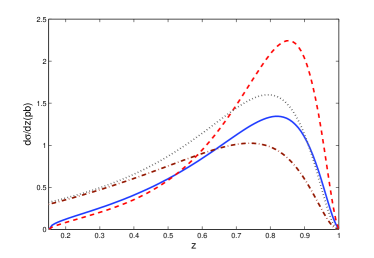
Figure 12: The differential cross sections $d\sigma/dz$ in $pb$ for the production of the doubly heavy baryons $\Xi_{bc}$, where $z$ is the energy fraction of the final baryon. The solid and dashed lines represent the contributions from ${|\left(bc\right){\scriptsize{}_{\overline{\textbf{3}}}}\,,^{1}S_{0}\rangle}$ and ${|\left(bc\right){\scriptsize{}_{\overline{\textbf{3}}}}\,,^{3}S_{1}\rangle}$ obtained by complete QCD approach, dash-dot and dot lines represent the contributions from ${|\left(bc\right){\scriptsize{}_{\overline{\textbf{3}}}}\,,^{1}S_{0}\rangle}$ and ${|\left(bc\right){\scriptsize{}_{\overline{\textbf{3}}}}\,,^{3}S_{1}\rangle}$ obtained by fragmentation approach.

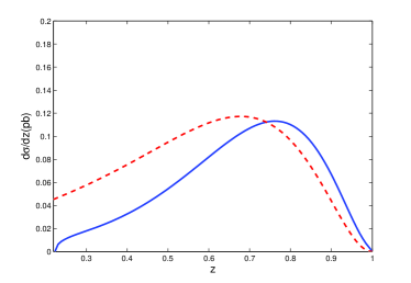
Figure 13: The differential cross sections $d\sigma/dz$ in $pb$ for the production of the doubly heavy baryons $\Xi_{bb}$, where $z$ is the energy fraction of the final baryon. The solid line represents the result obtained by complete QCD approach, dashed line represents that by fragmentation approach.

In FIGs.11,12,13 the energy fractions of $\Xi_{cc}$, $\Xi_{bc}$ and $\Xi_{bb}$ obtained by complete QCD calculation (LO) and fragmentation approach (LL) are presented respectively. For the results by fragmentation approach, the scale of the fragmentation functions have been evolved to $m_{Z}$. For $\Xi_{bc}$ production, the different diquark spin-state contributions are showed respectively in the figure. According to the analysis in $B_{c}$ meson production, for $\Xi_{bc}$ production, the contribtuions from $c$-quark fragmentation is very small, so we only present the contribtuion from $b$-quark fragmentation for $\Xi_{bc}$ production. From FIGs.11,12,13 one may see that the production of doubly heavy baryons at low energy fraction (small $z$) estimated by the fragmentation approach is greater than that by complete QCD approach, this is the same as we have observed in $B_{c}$ meson production.

IV Disscussions and conclusion

We, under two approaches, estimate the production of mesons $B_{c}$, its excited states $B_{c}(B^{*}_{c},\cdots)$ and doubly heavy baryons $\Xi_{cc}$, $\Xi_{bc}$, $\Xi_{bb}$ at a $Z$-factory with especial care on treating essential energy-scales of the production, and the results of the production on the total cross sections are consistent with the results on branching ratios for $Z$-boson decays to $B_{c}$ and $B^{*}_{c}$ up-to the next leading order (NLO) calculationsqiao . Whereas since we calculate the process $e^{+}+e^{-}\to B_{c}(B^{*}_{c})+\bar{c}+b$ instead of the $Z$-boson decays as in Ref.qiao , so we can obtain more properties of the production, such as the asymmetries shown in FIGs.2,8 and the production with polarized incoming beams shown in FIGs.3,4,9,10 besides the momentum fraction ($z$) distributions shown in FIGs.5,6,7 and FIGs.11,12,13 etc. These properties are important in studying the production of the doubly heavy hadrons. When all the experimental data are available, via comparisons of the data with the results obtained by the approaches, one may conclude which approach adopted here is better.

From the estimation here, one may expect that at a $Z$-factory with a luminosity such as $10^{34}cm^{-2}s^{-1}$ about a million of the $B_{c}$ mesons and doubly heavy baryons in ground-state may be produced per year, and when indirect production (to produce the excited states of them first and then by strong or electromagnetic interaction decays to transit to the ground states accordingly) is taken into account, then a few millions of $B_{c}$ mesons and the doubly heavy baryons in ground-state may be produced per year. Considering the fact that the efficiency of detecting the doubly heavy hadrons is quite small and the competition from LHCb etc, one may conclude that studies of the ground states may be OK (margin), but to discovery (to study of) the excited states of the doubly heavy hadrons etc, it would be better when the $Z$-factory’s luminosity is so high as $\sim 10^{35-36}cm^{-2}s^{-1}$.

Finally, in summary, several remarkable points on the production are collected as follows:

• To study the doubly heavy hadrons at an $e^{+}+e^{-}$ collider, only when its collision energy set at $Z$-pole with strong resonance effect, is practicable. When the collision energy deviates from $Z$-pole, the production cross sections decrease rapidly: when the collision energy deviates from $Z$-pole by $5$ GeV, the cross sections decrease just to about 10% of those at $Z$-pole; when collision energies at 180 GeV and 240 GeV, the cross sections of $B_{c}$ meson production become too small (in $fb$) to be observed.

• There are obvious backward-forward asymmetry in doubly heavy hadron productions. The backward-forward asymmetry comes from the parity violating in these processes involving the $Z^{0}$ exchange. In the productions of doubly heavy hadrons at Z-factory, the main contribution comes from the $Z^{0}$ exchange, so the backward-forward asymmetry is very obvious. This interesting property is observable at Z-factory.

• After summing the leading logarithm terms through the DGLAP equation, we obtain the energy distribution which is different from that obtained from the complete QCD calculation. Namely it predict more doubly heavy hadrons produced with lower energy fraction after evolving the scale to $m_{Z}$ in comparison with the prediction of the complete QCD prediction.

Acknowledgments: This work was supported in part by Nature Science Foundation of China (NSFC) under Grant No. 11275243, No. 11447601.

References

- (1) F. Abe, et al. (CDF Collaboration), Phys. Rev. Lett. 81, 2432 (1998); Phys. Rev. D 58, 112004 (1998).
- (2) T. Aaltonen, et al. (CDF Collaboration). Phys. Rev. D 87, 011101 (2013).
- (3) V.M. Abazov, et al. (D0 Collaboration), Phys. Rev. Lett. 101, 012001 (2008); Phys. Rev. Lett. 102, 092001 (2009).
- (4) R. Aaij, et al . (LHCb Collaboration), Phys. Rev. Lett. 109, 232001 (2012); 111, 181801 (2013); 114, 132001 (2015); Eur. Phys. J. C. 74, 2839 (2014); J. High Energy Phys. 09 075 (2013).
- (5) M. Mattson, et al. (SELEX Collaboration), Phys. Rev. Lett. 89, 112001 (2002).
- (6) M. A. Moinester, et al. (SELEX Collaboration), Czech. J. Phys. 53, B201 (2003).
- (7) A. Ocherashvili, et al. (SELEX Collaboration), Phys. Lett. B628, 18 (2005).
- (8) Z. Yang, X.-G. Wu, G. Chen, Q.-L. Liao and J.-W. Zhang, Phys. Rev. D85, 094015 (2012).
- (9) G. T. Bodwin, E. Braaten and G. P. Lepage, Phys. Rev. D 51, 1125 (1995) [Erratum-ibid. D 55, 5853 (1997)].
- (10) N. Brambilla, et al. Heavy Quarkonium Physics, CERN-2005-005 20 June 2005, arXiv: hep-ph/0412158; Heavy quarkonium: progress, puzzles, and opportunities, Eur. Phys. J. C 71, 1534 (2011) and references therein.
- (11) J.-P. Ma and C.-H. Chang, Sci. China-Phys. Mech. Astron., Preface: Z-Factory, 53: p-1947 (2010).
- (12) R. Barate, et al. (ALAPH Collaboration) Phys. Lett. B 402 213 (1997); P. Abreu, et al. (DELPHI Collaboration), Phys. Lett. B 398 207 (1997); K. Ackerstaff et al. (OPAL Collaboration), Phys. Lett. B 420 157 (1998).
- (13) E. Eichten, K. Gottfried, T. Kinoshita, K.D. Lane and T.M. Yan, Phys.Rev. D17, 3090(1978); ibid. 21, 313(E)(1980); ibid.21, 203(1980).
- (14) W. Buchmller and S.-H.H. Tye, Phys.Rev. D24, 132(1981).
- (15) A. Martin, Phys.Lett. B93, 338(1980).
- (16) C. Quigg and J.L. Rosner, Phys.Lett. B71, 153(1977).
- (17) Y.-Q. Chen and Y.-P. Kuang, Phys.Rev. D46, 1165(1992); Erratum-ibid. D47, 350(1993).
- (18) E.J. Eichten and C. Quigg, Phys.Rev. D49, 5845(1994).
- (19) C.-H. Chang and Y.-Q. Chen, Phys. Rev. D46, 3845(1992).
- (20) E. Braaten, K. Cheung and T.C. Yuan, Phys. Rev. D 48, R5049 (1993).
- (21) Y.-Q. Chen, Phys. Rev. D 48, 5181 (1993).
- (22) G. Altarelli and G. Parisi, Nucl.Phys. B126, 298(1977).
- (23) R.D .Field, Applications of Perturbative QCD, Addison-Wesley(1989).
- (24) C.-H. Chang, C.-F.Qiao, J.-X. Wang and X.-G. Wu, Phys.Rev. D70, 114019(2004).
- (25) J. Jiang, X.-G. Wu, Q.-L. Liao, X.-C. Zheng and Z.-Y. Fang, Phys. Rev. D86, 054021 (2012).
- (26) K.A Olive, et al. (Particle Data Group), Chin.Phys. C38, 090001(2014).
- (27) S.P. Baranov, Phys.Rev. D54, 3228(1996).
- (28) Cong-Feng Qiao, Li-Ping Sun, Rui-Lin Zhu, JHEP 1108, 131 (2011); Jun Jiang, Long-Bin Chen, Cong-Feng Qiao, Phys. Rev. D91, 034033 (2015).
- (29) C.-H. Chang and Y.-Q. Chen, Phys. Rev. D49, 3399(1994).