Quantum description of electromagnetic fields in waveguides

Abstract

Using quantum theory, we study the propagation of an optical field in an inhomogeneous dielectric, and apply this scheme to traveling optical fields in a waveguide. We introduce a field-atom interaction Hamiltonian and derive the refractive index using quantum optics. We show that the transmission and reflection of optical fields at an interface between different materials can be described with normalized Fresnel coefficients and that this representation is related to the beam splitter operator. We then study the propagation properties of the optical fields for two types of slab waveguides: step-index and graded-index. The waveguides are divided into multiple layers to represent the spatial dependence of the optical field. We can evaluate the number of photons in an arbitrary volume in the waveguide using this procedure. Using the present method, the quantum properties of weak optical fields in a waveguide are revealed, while coherent states with higher amplitudes reduces to representation of classical waveguide optics.

I Introduction

Currently, optical technology plays an important role in communication. To achieve long-distance communication, signals are transmitted through optical waveguides, which typically consist of silica-based glass.

The optical waveguide is a device used to achieve free propagation along its long axis and a confinement over its cross-section. Conventional optical waveguides consist of a core and cladding and can confine optical fields in the core because of the difference in indices. These optical waveguides are classified into two types: step-index (SI) and graded-index (GI). In particular, a waveguide of concentric structure is referred to as an optical fiber.

Conventionally, it is assumed that optical signals exhibit a certain amount of intensity in a waveguide, and the mathematical structure of the SI and GI waveguides has been very well studied within classical waveguide optics Snitzer (1961); Snyder and Love (1983). In addition, protocols using quantum interference among weak optical signals, referred to as quantum protocols, have recently been proposed Nielsen and Chuang (2000); Braunstein and Pati (2003). In these protocols, optical signals should be described using quantum optics. The optical waveguide is also considered an important device for long-distance propagation in quantum protocols, such as in quantum cryptography Gisin and Thew (2007); Sasaki et al. (2011).

Optical fields in a waveguide interact with dielectrics, and the interaction causes an effective decrease in light speed; this effect is phenomenologically introduced by a refractive index that is typically greater than or equal to unity. This process is discussed semi-classically in Feynman et al. (1965); Hecht (2001). Thus far, however, the quantization of optical waves traveling in a waveguide has not been discussed adequately. One of the few exceptions is the study in Drummond and Corney (2001). In this study, boundary effects in the waveguide were neglected, implying that the optical wave was assumed to travel along the core in a straight line. This assumption corresponds to a single-mode waveguide case. Strictly speaking, however, the optical wave in a waveguide shows spatial distribution over the cross-section, and the propagation property of the optical field is generally determined by the boundary condition at the interface between the core and cladding. In this sense, the spatial dependence of the optical field should also be considered when studying optical waveguides within quantum optics.

In this research, we study the propagation of the optical field in a dielectric such as silica-based glass from a quantum optics perspective and assume that the optical field is in a coherent state to allow comparison with the classical waveguide optics. First, we treat both the optical field and atom quantum theoretically and introduce an interaction Hamiltonian between them. Using quantum optics, we show that the refractive index can consistently be described as in a coherent state and that the electromagnetic field can be represented by this refractive index.

We also study transmission and reflection of optical fields at an interface between different materials. These properties are described by Fresnel coefficients in classical optics Hecht (2001), where, to satisfy the energy conservation law, the transmission coefficient is corrected by a factor that include refractive indices Hecht (1973); Zia (1988). Here as an alternative, we normalize electromagnetic fields and introduce normalized Fresnel coefficients. We show that this scheme is consistent with the representation of the beam splitter operator Barnett and Radmore (1997).

Following this, we discuss the propagation properties of optical fields in optical waveguides for SI and GI types. In both cases, the waveguides are divided into multiple layers, and the electromagnetic fields in each layer are described. This multi-layer division method enables us to represent the spatial dependence of the optical fields using quantum optics. Electromagnetic fields in adjacent layers are associated with each other using normalized Fresnel coefficients, and various propagation properties of the waveguides are studied. Here, we focus our attention on the linear properties of optical waveguides. We describe the quantum properties of optical fields in a waveguide for weak coherent states, while coherent states with higher amplitudes are reduced to a description in classical waveguide optics.

The rest of this paper is organized as follows. In Sec. II, we describe the propagation of the optical field in a dielectric. In Sec. III, from a quantum optics perspective, we consider the transmission and reflection of the optical fields at an interface between different materials. In Sec. IV, we study the propagation properties of the optical field in SI and GI optical waveguides. Section V presents the summary. Detailed derivations of the mathematical formulae used are presented in the appendices.

II Propagation of the optical field in a dielectric

II.1 Interaction-free Hamiltonian

Let us start with the vector potential as follows:

$$\hat{\bm{A}}_{l} = \sqrt{\frac{\hbar}{2\omega\varepsilon_{0}V}}\bigg{\{}\hat{a}_{l}^{\dagger}\exp[i(\omega t-\bm{k}_{l}\cdot\bm{r})]$$ (1)

$$\hskip 28.45274pt+\hat{a}_{l}\exp[-i(\omega t-\bm{k}_{l}\cdot\bm{r})]\bigg{\}}\bm{e}_{l},$$

where $\omega$ and $\varepsilon_{0}$ are the frequency of the optical field and the permittivity in vacuum, respectively, and $V=L_{x}L_{y}L_{z}$ is a unit volume, which is given later. The operators $\hat{a}_{l}^{\dagger}$ and $\hat{a}_{l}$ are the creation and annihilation operators in a mode $l$, respectively, and they satisfy the commutation relation

$$[\hat{a}_{l},\hat{a}_{l^{\prime}}^{\dagger}]=\delta_{ll^{\prime}}.$$ (2)

The vectors $\bm{k}_{l}$ and $\bm{e}_{l}$ are perpendicular to each other and are related to the wave vector and direction of polarization, respectively. For consistency with the later part, we employ $\bm{k}_{l}=\kappa_{l}\bm{e}_{x}+\beta_{l}\bm{e}_{z}$ and $\bm{e}_{l}=\bm{e}_{y}$. The magnitude of the vector $\bm{k}_{l}$ corresponds to the wave number in vacuum:

$$|\bm{k}_{l}|=\sqrt{\kappa_{l}^{2}+\beta_{l}^{2}}=k_{l}.$$ (3)

Considering the Coulomb gauge, we can obtain the electromagnetic fields thus

$$\hat{\bm{E}}_{l} = -\frac{\partial\hat{\bm{A}}_{l}}{\partial t}$$ (4a)

$$= -i\sqrt{\frac{\hbar\omega}{2\omega\varepsilon_{0}V}}[U_{tz}^{\ast}\hat{a}_{l}^{\dagger}\exp(-i\kappa_{l}x)$$

$$\hskip 42.67912pt-U_{tz}\hat{a}_{l}\exp(i\kappa_{l}x)]\bm{e}_{y},$$

$$\hat{\bm{H}}_{l} = \mu_{0}^{-1}(\nabla\times\hat{\bm{A}}_{l})$$ (4b)

$$= -\frac{i}{\mu_{0}}\sqrt{\frac{\hbar}{2\omega\varepsilon_{0}V}}[U_{tz}^{\ast}\hat{a}_{l}^{\dagger}\exp(-i\kappa_{l}x)$$

$$\hskip 42.67912pt-U_{tz}\hat{a}_{l}\exp(i\kappa_{l}x)](-\beta\bm{e}_{x}+\kappa_{l}\bm{e}_{z}),$$

where

$$U_{tz}=\exp[-i(\omega t-\beta_{l}z)]$$ (5)

is a temporal- and $z$-dependence. These electromagnetic fields propagate at light speed in vacuum along a direction parallel to $\bm{k}_{l}$, say $c$.

For the interaction-free case, equivalent to propagation in vacuum, the Hamiltonian is calculated using Eqs. (2), (4a), and (4b) as follows:

$$\hat{\mathcal{H}}_{l} = \int_{V}\left(\frac{\varepsilon_{0}}{2}\hat{\bm{E}}_{l}^{2}+\frac{\mu_{0}}{2}\hat{\bm{H}}_{l}^{2}\right)dV$$ (6)

$$= \hbar\omega\left(\hat{a}_{l}^{\dagger}\hat{a}_{l}+\frac{1}{2}\right)$$

Here, we can arbitrarily choose integration ranges along the $x$- and $y$-directions, for example, for $L_{x}=L_{y}=1$; a periodic boundary condition along the $z$-direction is considered.

$$L_{z}=\frac{2\pi n_{z}}{\beta_{l}}\quad(n_{z}=1,2,\cdots).$$ (7)

II.2 Field-atom interaction Hamiltonian

Following on, we study the case where the primary optical field interacts with an atom in a dielectric. The schematic is shown in Fig. 1.

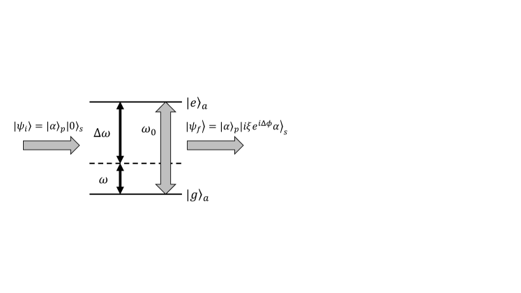
Figure 1: Field-atom interaction in an off-resonant regime. The atom has two energy-levels, $|g\rangle_{a}$ and $|e\rangle_{a}$, separated by frequency $\omega_{0}$. The atom is initially in the lower energy state $|g\rangle_{a}$, then the primary coherent field with frequency $\omega(\ll\omega_{0})$ comes in. The atom is virtually excited for a short time then soon de-excited. Via this interaction a secondary optical field, with a phase-shift of almost $\pi/2$, is generated in the same direction as the primary field.

As a result of this interaction, a secondary optical field is generated in the same direction as the primary field Hecht (2001). The modes of the primary and secondary fields are distinguished with indices $l=p,s$, respectively, and we have

$$\bm{k}_{p}=\bm{k}_{s}=\kappa\bm{e}_{x}+\beta\bm{e}_{z}.$$ (8)

We assume that the atom has two discrete states $|g\rangle_{a}$ and $|e\rangle_{a}$ separated by a frequency $\omega_{0}$, and that the atom is initially in the lower state $|g\rangle_{a}$. The free Hamiltonian of the optical fields is represented by Eq. (6) with $l=p,s$ and that of atom is given by Gerry and Knight (2005)

$$\hat{\mathcal{H}}_{a}=\frac{\hbar\omega_{0}}{2}\hat{\sigma}_{z},$$ (9)

where $\hat{\sigma}_{z}$ is a component of the Pauli spin-$\frac{1}{2}$ operator satisfying

$$\hat{\sigma}_{z}|e\rangle_{a} = |e\rangle_{a},$$ (10a)

$$\hat{\sigma}_{z}|g\rangle_{a} = -|g\rangle_{a},$$ (10b)

and let the total free Hamiltonian be

$$\hat{\mathcal{H}}_{0}=\hat{\mathcal{H}}_{p}+\hat{\mathcal{H}}_{s}+\hat{\mathcal{H}}_{a}.$$ (11)

We also assume that

$$\Delta\omega\equiv\omega_{0}-\omega\gg 0.$$ (12)

In this off-resonant situation the atom can be virtually excited in a short time permitted by the uncertainty relation,

$$\Delta\tau\sim\frac{1}{\Delta\omega}.$$ (13)

The atom is quickly de-excited, and it reverts to the $|g\rangle_{a}$ state. We assume that the primary optical field is in a coherent state $|\alpha\rangle_{p}$, and the initial state can be described as

$$|\psi_{i}\rangle=|\alpha\rangle_{p}|0\rangle_{s},$$ (14)

where the atomic state is not displayed because it remains at $|g\rangle_{a}$ before and after interaction.

Hereafter, we employ an approximation rule throughout this paper: small terms of the first order are included, while those of the second or higher orders are ignored. Regarding the interaction as a perturbation, we can write the effective interaction Hamiltonian in the interaction picture as follows (see Appendix A):

$$\hat{\mathcal{H}}_{\rm eff}\simeq-\hbar\chi(\hat{a}_{p}\hat{a}_{s}^{\dagger}+\hat{a}_{p}^{\dagger}\hat{a}_{s}),$$ (15)

where $\chi$ is proportional to the square of the field-atom coupling constant $g$ given in Eq. (84), and small terms of second or higher orders are not shown according to the approximation rule. The final state through the interaction is

$$|\psi_{f}\rangle=\exp\left(-i\frac{\hat{\mathcal{H}}_{\rm eff}}{\hbar}\Delta\tau\right)|\psi_{i}\rangle=|\alpha\rangle_{p}|i\xi\exp(i\delta)\alpha\rangle_{s},$$ (16)

where we used the relations in Appendix B and $\xi=\chi\Delta\tau$ is a small parameter. However, note that the leading term of the secondary mode is a small term of the first order, and that one of the second order should be considered here. It appears as a small phase $\delta$ that should be kept, even in the present approximation rule. This small phase, however, has no effect on the result because it disappears by multiplication with another small parameter. We can also see from Eq. (16) that the primary optical field is not attenuated at all within this approximation rule.

II.3 Expectation value of the composite field

The primary and secondary optical fields spatially overlap after the interaction. In the following discussion we study just the electric field but it is valid for both the electric and magnetic fields. We introduce the composite electric field as

$$\hat{\bm{E}}_{c}=\hat{\bm{E}}_{p}+\hat{\bm{E}}_{s},$$ (17)

where the suffix $c$ means a composite field. We obtain the expectation values of the optical field after the interaction with Eq. (16)

$$\bm{E}_{1}=\langle\psi_{f}|\hat{\bm{E}}_{c}|\psi_{f}\rangle=\bm{E}_{p}+\xi\bm{E}_{s},$$ (18)

where

$$\bm{E}_{l} = -i\sqrt{\frac{\hbar\omega}{2\varepsilon_{0}V}}[U_{tz}^{\ast}\alpha_{l}^{\ast}\exp(-i\kappa x)\exp(-i\phi_{l})$$ (19d)

$$\hskip 42.67912pt-U_{tz}\alpha_{l}\exp(i\kappa x)\exp(i\phi_{l})]\bm{e}_{y},$$

$$\phi_{l}=\left\{\begin{array}[]{cl}0&(l=p)\\ \frac{\pi}{2}+\delta&(l=s)\end{array}\right..$$

Here the suffix 1 in the left-hand side of Eq. (18) means that the interaction with an atom occurs once, and we also considered the relations Louisell (1973) as follows:

$$\exp(i\theta\hat{a}_{l}^{\dagger}\hat{a}_{l})|\alpha\rangle_{l}=|\alpha\exp(i\theta)\rangle_{l},$$ (20a)

$$\exp(-i\theta\hat{a}_{l}^{\dagger}\hat{a}_{l})\hat{a}_{l}\exp(i\theta\hat{a}_{l}^{\dagger}\hat{a}_{l})=\hat{a}_{l}\exp(i\theta)$$ (20b)

for an arbitrary real number $\theta$. In practice, both $\bm{E}_{p}$ and $\bm{E}_{s}$ propagate at light speed in vacuum, and have a common spatial period. However, the phase of the secondary field is delayed by almost $\pi/2$ compared with that of the primary. Therefore, these two fields destructively interfere with each other and a composite field, $\bm{E}_{1}$ with a spatial period identical to $\bm{E}_{p}$ and $\bm{E}_{s}$, is generated. Let the composite electric field be

$$\bm{E}_{1} = -i\mathcal{A}\sqrt{\frac{\hbar\omega}{2\varepsilon_{0}V}}[U_{tz}^{\ast}\alpha^{\ast}\exp(-i\kappa x)\exp(-i\delta\phi)$$ (21)

$$\hskip 42.67912pt-U_{tz}\alpha\exp(i\kappa x)\exp(i\delta\phi)]\bm{e}_{y}$$

with a constant $\mathcal{A}$ and a small phase $\delta\phi$.

Comparing Eqs. (18) and (21), we find $\mathcal{A}=1$ and $\delta\phi=\xi$ within the present approximation rule. This means that the amplitude of the composite field can be regarded as identical to the primary one and that the phase of the composite field is, when compared with $\bm{E}_{p}$, delayed by $\xi$ after the interaction with the atom. By substituting these parameters into Eq. (21), we obtain

$$\bm{E}_{1} = -i\sqrt{\frac{\hbar\omega}{2\varepsilon_{0}V}}\{\alpha^{\ast}\exp(i\omega t)\exp[-i(k_{0}r+\xi)]$$ (22)

$$\hskip 28.45274pt-\alpha\exp(-i\omega t)\exp[i(k_{0}r+\xi)]\},$$

where $r=x\cos\theta+z\sin\theta$ and $\tan\theta=\beta/\kappa$.

The optical field repeatedly interacts with subsequent atoms in the dielectric and the phase is delayed with each interaction. We assume that the atoms are aligned in an orderly manner at a distance $d$ apart on the propagation path of the optical field. We also assume that the optical field interacts with $m$ atoms within its spatial period and that the phase is totally delayed by $m\xi$ (Fig. 2). The total electric field is presented as

$$\bm{E}_{m} = -i\sqrt{\frac{\hbar\omega}{2\varepsilon_{0}V}}\{\alpha^{\ast}\exp(i\omega t)\exp[-i(k_{0}r+m\xi)]$$ (23)

$$\hskip 28.45274pt-\alpha\exp(-i\omega t)\exp[i(k_{0}r+m\xi)]\}.$$

This successive retardation in phase makes the wavelength of the composite field, say, $\lambda^{\prime}$ shorter than that of the primary field $\lambda$ .

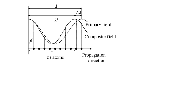
Figure 2: Retardation in phase caused by field-atom interactions. The secondary optical field with phase shifted is generated via an interaction, and the composition of the primary and secondary fields results in a phase retardation. The optical field interacts successively with $m$ atoms within the spatial period of the primary field, and the wavelength of the composite field consequently becomes shorter than that of primary by $\Delta\lambda$.

For the difference in wavelength $\Delta\lambda=\lambda-\lambda^{\prime}$, we have

$$k_{0}\Delta\lambda=m\xi.$$ (24)

Since from the assumption we find $m=\lambda^{\prime}/d$, we can obtain

$$\lambda^{\prime}=\frac{\lambda}{n},$$ (25)

where

$$n=1+\frac{\xi}{k_{0}d}>1$$ (26)

corresponds to the refractive index. From Eqs. (13), (84) and (90), and with the relation $k_{0}=\omega/c$, we can see that $n-1\propto(\Delta\omega)^{-2}$. This means that $n$ is an increasing function with respect to $\omega$ over the range $\omega\ll\omega_{0}$. This property agrees with Sellmeier’s dispersion formula Born and Wolf (1999).

From Eq. (25), the wave number in the dielectric accordingly becomes $k_{0}^{\prime}=nk_{0}$. Since the frequency $\omega$ stays unchanged during the interaction, we can regard the propagation speed of the composite field in the dielectric as $c^{\prime}=c/n<c$.

So far, from the perspective of quantum optics, we have described the refractive index as a parameter $n$ that characterizes the interaction between the optical field and the dielectric. Henceforth, we study the propagation property of the optical field in a dielectric using this parameter.

III Quantum treatment of the transmission and reflection of the optical field

In this section, we study the transmission and reflection of the optical field at an interface between different refractive indices from a quantum optics perspective.

III.1 Normalization of the Fresnel coefficients

We consider an interface with refractive indices $n_{j}$ and $n_{j^{\prime}}$. Two optical fields with indices $j+$ and $j^{\prime}-$ enter this interface from opposite sides with incident angles of $\theta_{j}$ and $\theta_{j^{\prime}}$, respectively, and interfere with each other. As a result, another two optical fields of indices $j-$ and $j^{\prime}+$ exit the interface (Fig. 3). Here ’$j+$ ’ and ’$j-$’ denote that the positive and negative $x$-component of the wave vector in an area $j$, respectively.

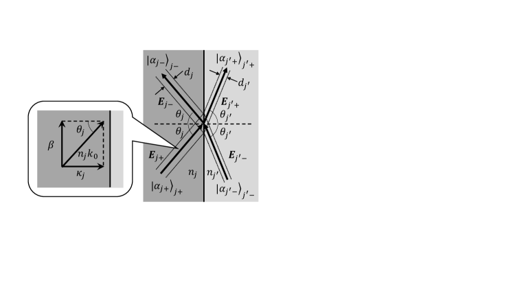
Figure 3: Interactions among electric fields at an interface between different materials. Electric fields $j+$ and $j^{\prime}-$ enter with incident angles $\theta_{j}$ and $\theta_{j^{\prime}}$, respectively, and those of $j^{\prime}+$ and $j-$ exit. Widths of the optical beams in the areas $j$ and $j^{\prime}$ are denoted by $d_{j}$ and $d_{j^{\prime}}$, respectively.

We assume that the electric field is polarized in a direction parallel to the interface, which is the $y$-axis (TE mode), and that the wave vectors are given by $\bm{k}_{j\pm}=\kappa_{j}\bm{e}_{x}\pm\beta\bm{e}_{z}$ and $\bm{k}_{j^{\prime}\pm}=\kappa_{j^{\prime}}\bm{e}_{x}\pm\beta\bm{e}_{z}$, with double-sign in same order. Among the components of the wave vectors, the relation

$$\kappa_{i}^{2}+\beta^{2}=(n_{i}k_{0})^{2}$$ (27)

holds for $i=j,j^{\prime}$. Note that the $z$-component values are identical in all four optical fields according to Snell’s law. The electromagnetic fields, that is, $\hat{\bm{E}}_{j\pm}$ and $\hat{\bm{H}}_{j\pm}$, are given with double-sign notation as follows:

$$\hat{\bm{E}}_{j\pm} = -i\sqrt{\frac{\hbar\omega}{2\varepsilon_{0}V}}[U_{tz}^{\ast}\hat{a}_{j\pm}^{\dagger}\exp(\mp i\kappa_{j}x)$$ (28a)

$$\hskip 5.69054pt-U_{tz}\hat{a}_{j\pm}\exp(\pm i\kappa_{j}x)]\bm{e}_{y},$$

$$\hat{\bm{H}}_{j\pm} = -\frac{i}{\mu_{0}}\sqrt{\frac{\hbar}{2\omega\varepsilon_{0}V}}[U_{tz}^{\ast}\hat{a}_{j\pm}^{\dagger}\exp(\mp i\kappa_{j}x)$$ (28b)

$$\hskip 5.69054pt-U_{tz}\hat{a}_{j\pm}\exp(\pm i\kappa_{j}x)](-\beta\bm{e}_{x}\pm\kappa_{j}\bm{e}_{z}),$$

Classical electromagnetic fields correspond to the expectation values of the above operators when in a coherent state, that is,

$$\bm{E}_{j\pm} = {}_{j\pm}\langle\alpha_{j\pm}|\hat{\bm{E}}_{j\pm}|\alpha_{j\pm}\rangle_{j\pm},$$ (29a)

$$\bm{H}_{j\pm} = {}_{j\pm}\langle\alpha_{j\pm}|\hat{\bm{H}}_{j\pm}|\alpha_{j\pm}\rangle_{j\pm},$$ (29b)

where $\hat{a}_{j\pm}|\alpha_{j\pm}\rangle_{j\pm}=\alpha_{j\pm}|\alpha_{j\pm}\rangle_{j\pm}$ with double-sign notation.

In an ordinary procedure, tangential components of electromagnetic fields must be continuous at the interface Hecht (2001). We obtain Fresnel coefficients that are the ratios of the amplitude of the transmitted or reflected electromagnetic fields to the incident ones. In this conventional formulation, the energy density per unit time of the input and output optical fields are not conserved at the interface. This is because the following factors are not considered; first, as stated in the previous section, the ratio of the effective light-speed in areas $j$ and $j^{\prime}$ is $n_{j}^{-1}:n_{j^{\prime}}^{-1}$, and second, the cross-section of the transmitted optical field is different from that of the incident field due to refraction. The energy density is proportional to the inverse of the cross-section. With a unit length along the $y$-direction, thus the ratio of energy density is $d_{j}^{-1}:d_{j^{\prime}}^{-1}=n_{j}/\kappa_{j}:n_{j^{\prime}}/\kappa_{j^{\prime}}$ because $d_{i}\propto\cos\theta_{i}=\kappa_{i}/(n_{i}k_{0})$ for $i=j,j^{\prime}$. As a consequence, the ratio of the energy density in areas $j$ and $j^{\prime}$ is $\kappa_{j}^{-1}:\kappa_{j^{\prime}}^{-1}$ per unit time. To conserve energy density in the conventional procedure the transmission coefficient is multiplied by a correction factor Hecht (1973); Zia (1988).

Here we use another technique; normalization of the electromagnetic field in area $j$ by a factor $\kappa_{j}^{-1/2}$.

$$\left.\frac{(E_{j+})_{y}+(E_{j-})_{y}}{\sqrt{\kappa_{j}}}\right|_{x=\xi_{jj^{\prime}}} = \left.\frac{(E_{j^{\prime}+})_{y}+(E_{j^{\prime}-})_{y}}{\sqrt{\kappa_{j^{\prime}}}}\right|_{x=\xi_{jj^{\prime}}},$$

$$\left.\frac{(H_{j+})_{z}+(H_{j-})_{z}}{\sqrt{\kappa_{j}}}\right|_{x=\xi_{jj^{\prime}}} = \left.\frac{(H_{j^{\prime}+})_{z}+(H_{j^{\prime}-})_{z}}{\sqrt{\kappa_{j}^{\prime}}}\right|_{x=\xi_{jj^{\prime}}},$$

where $(E_{j\pm})_{y}$ and $(H_{j\pm})_{z}$ are the $y$- and $z$-components of operators $\bm{E}_{j\pm}$ and $\bm{H}_{j\pm}$, respectively, and $\xi_{jj^{\prime}}$ is the position of the interface. Using electromagnetic fields similar to Eqs. (4a) and (4b) and the wave vectors introduced before, eigenvalues $\alpha_{j\pm},\alpha_{j^{\prime}\pm}$ are related to the normalized Fresnel coefficients as follows :

$$\left(\begin{array}[]{c}\alpha_{j^{\prime}+}\\ \alpha_{j-}\end{array}\right)=\left(\begin{array}[]{cc}\tilde{t}_{jj^{\prime}}&-\tilde{r}_{jj^{\prime}}\\ \tilde{r}_{jj^{\prime}}&\tilde{t}_{jj^{\prime}}\end{array}\right)\left(\begin{array}[]{c}\alpha_{j+}\\ \alpha_{j^{\prime}-}\end{array}\right),$$ (31)

where

$$\tilde{t}_{jj^{\prime}} = \frac{2\sqrt{\kappa_{j}\kappa_{j^{\prime}}}}{\kappa_{j}+\kappa_{j^{\prime}}},$$ (32a)

$$\tilde{r}_{jj^{\prime}} = \frac{\kappa_{j}-\kappa_{j^{\prime}}}{\kappa_{j}+\kappa_{j^{\prime}}}$$ (32b)

and the phase factor $\exp(\pm i\kappa_{j}\xi_{jj^{\prime}})$ is renormalized in the operators of the area $j$, that is, $\alpha_{j\pm}\rightarrow\alpha_{j\pm}\exp(\mp i\kappa_{j}\xi_{jj^{\prime}})$. It is clear from Eqs. (32a) and (32b) that $\tilde{t}_{jj^{\prime}}^{2}+\tilde{r}_{jj^{\prime}}^{2}=1$ holds.

Introducing $|\psi\rangle=|\alpha_{j+}\rangle_{j+}|\alpha_{j-}\rangle_{j-}|\alpha_{j^{\prime}+}\rangle_{j^{\prime}+}|\alpha_{j^{\prime}-}\rangle_{j^{\prime}-}$, which satisfies $\hat{a}_{i\pm}|\psi\rangle=\alpha_{i\pm}|\psi\rangle$ for $i=j,j^{\prime}$, we rewrite Eq. (31) as follows:

$$\langle\psi|\left(\begin{array}[]{c}\hat{a}_{j^{\prime}+}\\ \hat{a}_{j-}\end{array}\right)|\psi\rangle = \langle\psi|\left(\begin{array}[]{cc}\tilde{t}_{jj^{\prime}}&-\tilde{r}_{jj^{\prime}}\\ \tilde{r}_{jj^{\prime}}&\tilde{t}_{jj^{\prime}}\end{array}\right)\left(\begin{array}[]{c}\hat{a}_{j+}\\ \hat{a}_{j^{\prime}-}\end{array}\right)|\psi\rangle$$ (39)

$$= \langle\psi|\hat{\mathcal{U}}_{jj^{\prime}}\left(\begin{array}[]{c}\hat{a}_{j+}\\ \hat{a}_{j^{\prime}-}\end{array}\right)\hat{\mathcal{U}}_{jj^{\prime}}^{\dagger}|\psi\rangle,$$ (42)

where

$$\hat{\mathcal{U}}_{jj^{\prime}}=\exp[\vartheta_{jj^{\prime}}(\hat{a}_{j+}^{\dagger}\hat{a}_{j^{\prime}-}-\hat{a}_{j+}\hat{a}_{j^{\prime}-}^{\dagger})],$$ (43)

is the beam splitter operator (see Appendix B). Here, $\vartheta_{jj^{\prime}}$ is a real parameter and is related to the normalized Fresnel coefficients as $\tan\vartheta_{jj^{\prime}}=\tilde{r}_{jj^{\prime}}/\tilde{t}_{jj^{\prime}}$. The parameter $\vartheta_{jj^{\prime}}$ should be distinguished from the incident and refraction angles, $\theta_{j}$ and $\theta_{j^{\prime}}$. Equation (42) shows the relation between the operators of the optical fields.

$$\hat{a}_{j^{\prime}+} = \hat{\mathcal{U}}_{jj^{\prime}}\hat{a}_{j+}\hat{\mathcal{U}}_{jj^{\prime}}^{\dagger},$$ (44a)

$$\hat{a}_{j-} = \hat{\mathcal{U}}_{jj^{\prime}}\hat{a}_{j^{\prime}-}\hat{\mathcal{U}}_{jj^{\prime}}^{\dagger}.$$ (44b)

The state after interference is obtained by transforming Eq. (43).

$$|\alpha_{j+}\rangle_{j+}|\alpha_{j^{\prime}-}\rangle_{j^{\prime}-}\rightarrow\hat{\mathcal{U}}_{jj^{\prime}}|\alpha_{j+}\rangle_{j^{\prime}+}|\alpha_{j^{\prime}-}\rangle_{j-}$$

$$= |\tilde{t}_{jj^{\prime}}\alpha_{j+}+\tilde{r}_{jj^{\prime}}\alpha_{j^{\prime}-}\rangle_{j^{\prime}+}|-\tilde{r}_{jj^{\prime}}\alpha_{j+}+\tilde{t}_{jj^{\prime}}\alpha_{j^{\prime}-}\rangle_{j-},$$

where $\tilde{t}_{jj^{\prime}}=\cos\vartheta_{jj^{\prime}}$ and $\tilde{r}_{jj^{\prime}}=\sin\vartheta_{jj^{\prime}}$ are considered. It is clear that we obtain $\tilde{t}_{jj^{\prime}}=1$ and $\tilde{r}_{jj^{\prime}}=0$ when $n_{j^{\prime}}=n_{j}$. This special case means that the optical field travels in a straight line in a homogeneous dielectric, without refraction.

The normalized Fresnel coefficients are related to the conventional Fresnel coefficients in a simple way,

$$\tilde{t}_{jj^{\prime}} = \sqrt{\frac{\kappa_{j^{\prime}}}{\kappa_{j}}}t_{jj^{\prime}}=\sqrt{\frac{\kappa_{j}}{\kappa_{j^{\prime}}}}t^{\prime}_{jj^{\prime}},$$ (46a)

$$\tilde{r}_{jj^{\prime}} = r_{jj^{\prime}}=-r^{\prime}_{jj^{\prime}}$$ (46b)

for the coefficients $t_{jj^{\prime}}$ ($t^{\prime}_{jj^{\prime}}$) related to the transmission $j+\rightarrow j^{\prime}+$ ($j^{\prime}-\rightarrow j-$) and $r_{jj^{\prime}}$ ($r^{\prime}_{jj^{\prime}}$) related to the reflection $j+\rightarrow j-$ ($j^{\prime}-\rightarrow j^{\prime}+$).

III.2 Total reflection case

Another special case is when the optical field $j$ comes in at the critical angle

$$\theta_{c}=\sin^{-1}(n_{j^{\prime}}/n_{j})$$ (47)

for $n_{j}>n_{j^{\prime}}$. This is the well-known total reflection case, and the refraction angle is $\theta_{j^{\prime}}=\pi/2$. This means that the lateral component of the wave vector in area $j^{\prime}$ vanishes as $\kappa_{j^{\prime}}=0$. In this case, we can easily calculate $\tilde{t}_{jj^{\prime}}=0$ and $\tilde{r}_{jj^{\prime}}=1$ from Eqs. (32a) and (32b). When $\theta_{c}<\theta<\pi/2$, the refraction angle is mathematically shown as $\theta_{j^{\prime}}=\pi/2-i\varphi_{j^{\prime}}$ with a real number $\varphi_{j^{\prime}}$ Navasquillo et al. (1989). We then have

$$\kappa_{j^{\prime}}=n_{j^{\prime}}k_{0}\cos\theta_{j^{\prime}}=in_{j^{\prime}}k_{0}\sinh\varphi_{j^{\prime}}\equiv i\gamma_{j^{\prime}}.$$ (48)

The real and imaginary part of the wave vector is related to the wave number and effective loss, respectively Lodenquai (1991), and Eq. (48) shows that the wave number along the $x$-direction is zero in area $j^{\prime}$. This means that we can also regard $\kappa_{j^{\prime}}$ as zero in Eqs. (32a) and (32b) and again we find the total reflection case.

So far, according to the present model, no optical field exists in the area $j^{\prime}$ because it is totally reflected at the interface. In practice, however, a certain amount of the optical field, as far as the wavelength distance, can leak in to area $j^{\prime}$. This leakage is referred to as the evanescent field Snyder and Love (1983) and we can clarify it using the uncertainty relation. As stated above, for the total reflection case, the incident angle satisfies the inequality $\theta_{c}\leq\theta_{j}<\pi/2$. The inequality is reduced to

$$0<\kappa_{j}\leq\kappa_{c}=n_{j}k_{0}\cos\theta_{c}$$ (49)

with an $x$-component of the wave vector in area $j$. This inequality (49) shows that the totally reflected optical field displays a fluctuation $\Delta\kappa_{j}=\kappa_{c}$. Using de Broglie’s relation,

$$\Delta p_{x}=\hbar\Delta\kappa_{j}=k_{0}\sqrt{n_{j}^{2}-n_{j^{\prime}}^{2}},$$ (50)

where Eq. (47) is also considered. From the uncertainty relation,

$$\Delta q_{x}\simeq\frac{\hbar}{\Delta p_{x}}=\frac{\lambda_{0}}{2\pi n_{j}\sqrt{2\Delta_{r}}},$$ (51)

where $\lambda_{0}=2\pi/k_{0}$ is the wave length of the optical field in vacuum and

$$\Delta_{r}=\frac{n_{j}^{2}-n_{j^{\prime}}^{2}}{2n_{j}^{2}}$$ (52)

is the relative index difference. Introducing $n_{j}=1.45$ and $\Delta_{r}=0.01$ as typical parameters, we obtain $\Delta q_{x}\simeq\lambda_{0}/1.29$. This result shows that the optical field can proceed into the area prohibited by the total reflection scheme, by the degree of a wavelength.

IV Propagation of the optical field in slab waveguides

In the previous sections, we studied the propagation of an optical field in a homogeneous dielectric and its behavior at an interface. By combining these procedures, we can describe the behavior of optical fields in an inhomogeneous dielectric, such as waveguides.

IV.1 Step-index slab waveguide

The simplest example is the step-index (SI) slab waveguide. It consists of a homogeneous core and cladding, with refractive indices of $n_{1}$ and $n_{2}(<n_{1})$, respectively. The waveguide propagates the optical field along the longitudinal direction and confines it within the cross section. This mechanism is achieved by total (internal) reflection at the core-cladding interface.

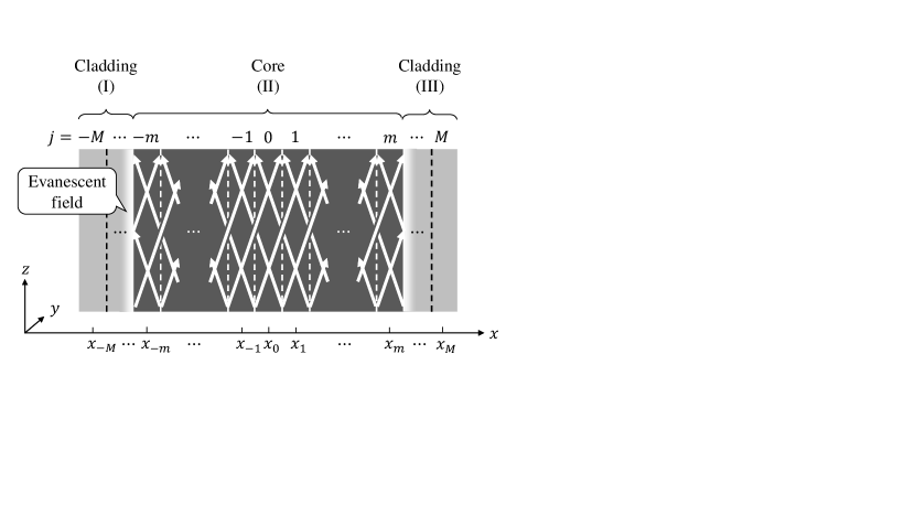
Figure 4: Step-index slab waveguide in a symmetric structure. The core and cladding are divided into layers with a common thickness $\Delta x$ representing the spatial dependence of the optical field. The optical field is chiefly confined in the core, but part of it leaks to the cladding as an evanescent field.

A schematic of the SI slab waveguide is shown in Fig. 4. Here, a symmetrical structure, where refractive indices of left- and right-side cladding are identical, is considered. To represent the spatial dependence of the optical field in the waveguide, the core and cladding are divided into stacked layers, the thicknesses of which is denoted by $\Delta x$. The order of layers is distinguished by an index $j$, and the $j$th layer is located in the range

$$\left(j-\frac{1}{2}\right)\Delta x\leq x\leq\left(j+\frac{1}{2}\right)\Delta x.$$ (53)

We assume that the core and cladding correspond to areas $|j|\leq m$ and $m+1\leq|j|\leq M$, respectively. We introduce the center position of the $j$th layer as

$$x_{j}=j\Delta x.$$ (54)

Let the position of the core-cladding interface be $x=x_{\pm m}\pm\Delta x/2=\pm d/2$, where double-sign in same order is assumed. For convenience we refer to the left cladding, core, and right cladding as areas (I), (II), and (III), respectively.

The optical field in the cladding is distributed as an evanescent field. The $x$-component of wave vector of the evanescent field is given by an imaginary number as shown in Eq. (48). This means that the wave vector can be complex. Since the operator corresponding to the electromagnetic field should be Hermitian, we introduce the vector potential in the SI slab waveguide as

$$\hat{\bm{A}}_{j} = \sqrt{\frac{\hbar}{2\omega\varepsilon_{0}V_{j}}}\Big{\{}\hat{a}_{j}^{\dagger}\exp[i(\omega t-\bm{k}_{j}^{\ast}\cdot\bm{r})]$$ (55)

$$\hskip 56.9055pt+\hat{a}_{j}\exp[-i(\omega t-\bm{k}_{j}\cdot\bm{r})]\Big{\}}\bm{e}_{y},$$

with $V_{j}=\Delta x\cdot 1\cdot 2\pi n_{z}/\beta$. The asterisk in Eq. (55) shows the complex conjugate. This vector potential gives the electromagnetic fields of a TE mode. In areas (I), (II), and (III) wave vectors are given by

$$\bm{k}^{\rm(I)}_{j} = -i\gamma\bm{e}_{x}+\beta\bm{e}_{z},$$ (56a)

$$\bm{k}^{\rm(II)}_{j\pm} = \pm\kappa\bm{e}_{x}+\beta\bm{e}_{z},$$ (56b)

$$\bm{k}^{\rm(III)}_{j} = i\gamma\bm{e}_{x}+\beta\bm{e}_{z},$$ (56c)

respectively. It is clear that the absolute values of the $x$-components of $\bm{k}^{\rm(I)}_{j}$ and $\bm{k}^{\rm(III)}_{j}$ are identical because the structure of the waveguide is symmetrical and the incident angles at the interfaces between the core and cladding are identical. Optical fields with $x$-components of $\pm\kappa$ are shown by a double-sign notation in $\bm{k}^{\rm(II)}_{j\pm}$. These fields are spatially superposed resulting in a sinusoidal distribution in the core. Note that, at the interface between adjacent layers, optical fields travel with no interaction because the core is assumed to be homogeneous and the normalized Fresnel coefficient for the transmission is unity.

The vector potentials in areas (I), (II), and (III) are defined as follows:

$$\hat{\bm{A}}_{j}^{\rm(I)} = \sqrt{\frac{\hbar}{2\omega\varepsilon_{0}V_{j}}}(U_{tz}^{\ast}\hat{a}_{j}^{{\rm(I)}\dagger}+U_{tz}\hat{a}_{j}^{\rm(I)})\exp(\gamma x)\bm{e}_{y}$$ (57a)

$$\hskip 71.13188pt(-M\leq j\leq-m-1),$$

$$\hat{\bm{A}}_{j}^{\rm(II)} = \frac{\hat{\bm{A}}_{j+}^{\rm(II)}+\hat{\bm{A}}_{j-}^{\rm(II)}}{\sqrt{2}}\quad(-m\leq j\leq m),$$ (57b)

$$\hat{\bm{A}}_{j}^{\rm(III)} = \sqrt{\frac{\hbar}{2\omega\varepsilon_{0}V_{j}}}(U_{tz}^{\ast}\hat{a}_{j}^{{\rm(III)}\dagger}+U_{tz}\hat{a}_{j}^{\rm(III)})\exp(-\gamma x)\bm{e}_{y}$$ (57c)

$$\hskip 71.13188pt(m+1\leq j\leq M),$$

where $U_{tz}=\exp[-i(\omega t-\beta z)]$ is a temporal- and $z$-dependence similar to Eq. (5) and

$$\hat{\bm{A}}_{j\pm}^{(\rm II)} = \sqrt{\frac{\hbar}{2\omega\varepsilon_{0}V_{j}}}[U_{tz}^{\ast}\hat{a}_{j\pm}^{{\rm(II)}\dagger}\exp(\mp i\kappa x)$$ (58)

$$\hskip 56.9055pt+U_{tz}\hat{a}_{j\pm}^{\rm(II)}\exp(\pm i\kappa x)]\bm{e}_{y}$$

with double-sign in same order. Here, $\hat{a}_{j\pm}$ is the operator for the optical field with the wave vector (56b). Similar to Eqs. (4a) and (4b), the electromagnetic fields in each area are calculated thus:

$$\hat{\bm{E}}_{j}^{\rm(I)} = -i\sqrt{\frac{\hbar\omega}{2\varepsilon_{0}V_{j}}}(U_{tz}^{\ast}\hat{a}_{j}^{{\rm(I)}\dagger}-U_{tz}\hat{a}_{j}^{\rm(I)})\exp(\gamma x)\bm{e}_{y},$$ (59a)

$$\hat{\bm{E}}_{j}^{\rm(II)} = \frac{\hat{\bm{E}}_{j+}^{\rm(II)}+\hat{\bm{E}}_{j-}^{\rm(II)}}{\sqrt{2}},$$ (59b)

$$\hat{\bm{E}}_{j}^{\rm(III)} = -i\sqrt{\frac{\hbar\omega}{2\varepsilon_{0}V_{j}}}(U_{tz}^{\ast}\hat{a}_{j}^{{\rm(III)}\dagger}-U_{tz}\hat{a}_{j}^{\rm(III)})\exp(-\gamma x)\bm{e}_{y},$$

$$\hat{\bm{H}}_{j}^{\rm(I)} = -\frac{i}{\mu_{0}}\sqrt{\frac{\hbar}{2\omega\varepsilon_{0}V_{j}}}[-\beta(U_{tz}^{\ast}\hat{a}_{j}^{{\rm(I)}\dagger}-U_{tz}\hat{a}_{j}^{\rm(I)})\bm{e}_{x}$$ (59d)

$$\hskip 28.45274pt+i\gamma(U_{tz}^{\ast}\hat{a}_{j}^{{\rm(I)}\dagger}+U_{tz}\hat{a}_{j}^{\rm(I)})\bm{e}_{z}]\exp(\gamma x),$$

$$\hat{\bm{H}}_{j}^{\rm(II)} = \frac{\hat{\bm{H}}_{j+}^{\rm(II)}+\hat{\bm{H}}_{j-}^{\rm(II)}}{\sqrt{2}},$$ (59e)

$$\hat{\bm{H}}_{j}^{\rm(III)} = -\frac{i}{\mu_{0}}\sqrt{\frac{\hbar}{2\omega\varepsilon_{0}V_{j}}}[-\beta(U_{tz}^{\ast}\hat{a}_{j}^{{\rm(III)}\dagger}-U_{tz}\hat{a}_{j}^{\rm(III)})\bm{e}_{x}$$

$$\hskip 28.45274pt-i\gamma(U_{tz}^{\ast}\hat{a}_{j}^{{\rm(III)}\dagger}+U_{tz}\hat{a}_{j}^{\rm(III)})\bm{e}_{z}]\exp(-\gamma x),$$

where

$$\hat{\bm{E}}_{j\pm}^{\rm(II)} = -i\sqrt{\frac{\hbar\omega}{2\varepsilon_{0}V_{j}}}[U_{tz}^{\ast}\hat{a}_{j\pm}^{{\rm(II)}\dagger}\exp(\mp i\kappa x)$$ (60a)

$$\hskip 14.22636pt-U_{tz}\hat{a}_{j\pm}^{\rm(II)}\exp(\pm i\kappa x)]\bm{e}_{y},$$

$$\hat{\bm{H}}_{j\pm}^{\rm(II)} = -\frac{i}{\mu_{0}}\sqrt{\frac{\hbar}{2\omega\varepsilon_{0}V_{j}}}[U_{tz}^{\ast}\hat{a}_{j\pm}^{{\rm(II)}\dagger}\exp(\mp i\kappa x)$$ (60b)

$$\hskip 14.22636pt-U_{tz}\hat{a}_{j\pm}^{\rm(II)}\exp(\pm i\kappa x)](-\beta\bm{e}_{x}\pm\kappa\bm{e}_{z})$$

with double-sign in same order.

Here we introduce a spatially-averaged operator in the $j$th layer. For areas (I), (II), and (III), we have

$$c^{\rm(I)}_{j} = \frac{1}{\Delta x}\int_{(j-\frac{1}{2})\Delta x}^{(j+\frac{1}{2})\Delta x}\hat{a}^{\rm(I)}_{j}\exp(\gamma x)dx$$ (61a)

$$\simeq \hat{a}_{j}^{\rm(I)}\exp(\gamma x_{j}),$$

$$\hat{c}_{j}^{\rm(II)} = \frac{1}{\Delta x}\int_{(j-\frac{1}{2})\Delta x}^{(j+\frac{1}{2})\Delta x}\frac{\hat{a}_{j+}^{\rm(II)}\exp(i\kappa x)+\hat{a}_{j-}^{\rm(II)}\exp(-i\kappa x)}{\sqrt{2}}dx$$ (61b)

$$\simeq \frac{\hat{a}_{j+}^{\rm(II)}\exp(i\kappa x_{j})+\hat{a}_{j-}^{\rm(II)}\exp(-i\kappa x_{j})}{\sqrt{2}},$$

$$c^{\rm(III)}_{j} = \frac{1}{\Delta x}\int_{(j-\frac{1}{2})\Delta x}^{(j+\frac{1}{2})\Delta x}\hat{a}^{\rm(III)}_{j}\exp(-\gamma x)dx$$ (61c)

$$\simeq \hat{a}_{j}^{\rm(III)}\exp(-\gamma x_{j})$$

with a small $\Delta x$. In area (II) in particular, this spatially-averaged operator characterizes a standing wave formed by the interference between the electric (magnetic) fields $\hat{\bm{E}}_{j+}^{\rm(II)}$ and $\hat{\bm{E}}_{j-}^{\rm(II)}$ ($\hat{\bm{H}}_{j+}^{\rm(II)}$ and $\hat{\bm{H}}_{j+}^{\rm(II)}$). It is obvious that the spatially-averaged operator $\hat{c}_{j}^{\rm(K)}(\textrm{K}=\textrm{I},\textrm{II},\textrm{III})$ satisfies a commutation relation:

$$[\hat{c}^{\rm(I)}_{j},\hat{c}^{{\rm(I)}\dagger}_{j}]=\exp(2\gamma x_{j}),$$ (62a)

$$[\hat{c}_{j}^{\rm(II)},\hat{c}_{j}^{{\rm(II)}\dagger}]=1,$$ (62b)

$$[\hat{c}^{\rm(III)}_{j},\hat{c}^{{\rm(III)}\dagger}_{j}]=\exp(-2\gamma x_{j}).$$ (62c)

The right-hand side of Eqs. (62a) and (62c) are not unity because the optical fields in areas (I) and (III) are the evanescent fields, respectively.

We can evaluate the number of photons in the $j$th layer with spatially-averaged operators: $\hat{N}^{\rm(K)}_{j}=\hat{c}^{{\rm(K)}\dagger}_{j}\hat{c}^{\rm(K)}_{j}(\textrm{K}=\textrm{I},\textrm{II},\textrm{III})$. The momentum of the field in the area (K) is calculated by the $z$-component of the Poynting vector for a small $\Delta x$ Louisell (1973).

$$\left.\hat{G}^{\rm(K)}_{j}\right|_{z} = \frac{1}{c^{2}}\int(\hat{\bm{E}}^{\rm(K)}_{j}\times\hat{\bm{H}}^{\rm(K)}_{j})\cdot\bm{e}_{z}dV$$ (63)

$$\simeq \frac{\hbar\beta}{2}(\hat{c}^{\rm(K)}_{j}\hat{c}^{{\rm(K)}\dagger}_{j}+\hat{c}^{{\rm(K)}\dagger}_{j}\hat{c}^{\rm(K)}_{j}),$$

where the above integration is calculated over the unit volume of the $j$th layer $V_{j}$ for a small $\Delta x$. Using the commutation relation, it is clear that energy flow in the $j$th layer is proportional to the number of photons in the $j$th layer. Total momentum in the waveguide is obtained by

$$\hat{G}_{z}=\sum_{j=-M}^{M}\left.\hat{G}^{\rm(K)}_{j}\right|_{z}.$$ (64)

This operator is related to the energy flow along the $z$-direction and is discussed later.

Let us consider the expectation values of electromagnetic fields. In the present scheme, we assume that the field is in a coherent state over the complete cross-section of the optical waveguide. This assumption is valid because the distribution of the electromagnetic field is static in cross-section in SI optical waveguides. The total state of the optical field is described as

$$|\alpha\rangle=\bigotimes_{j=-M}^{M}|\alpha^{\rm(K)}_{j}\rangle_{j},$$ (65)

where $\textrm{K}=\textrm{I}$ for $-M\leq j\leq-m-1$, $\textrm{K}=\textrm{II}$ for $-m\leq j\leq m$, and $\textrm{K}=\textrm{III}$ for $m+1\leq j\leq M$. Note that, in area (II), we should distinguish optical fields with wave vectors $\bm{k}^{\rm(II)}_{j\pm}$ as different spatial modes, then we have $|\alpha^{\rm(II)}_{j}\rangle_{j}=|\alpha^{\rm(II)}_{j+}\rangle_{j+}\otimes|\alpha^{\rm(II)}_{j-}\rangle_{j-}$.

Also, we introduce eigenvalues for coherent state optical field operator. For each area,

$$\hat{a}_{j}^{\rm(K)}|\alpha_{j}^{\rm(K)}\rangle_{j} = \alpha_{j}^{\rm(K)}|\alpha_{j}^{\rm(K)}\rangle_{j}\quad(\textrm{K}=\textrm{I},\textrm{III}),$$ (66a)

$$\hat{a}_{j\pm}^{\rm(II)}|\alpha_{j\pm}^{\rm(II)}\rangle_{j\pm} = \alpha_{j\pm}^{\rm(II)}|\alpha_{j\pm}^{\rm(II)}\rangle_{j\pm}$$ (66b)

with double-sign in same order. We can obtain expectation values of electromagnetic fields in the $j$th layer as follows for $\textrm{K}=\textrm{I},\textrm{II},\textrm{III}$:

$$\bm{E}_{j}^{\rm(K)} = {}_{j}\langle\alpha^{\rm(K)}_{j}|\hat{\bm{E}}_{j}^{\rm(K)}|\alpha^{\rm(K)}_{j}\rangle_{j},$$ (67a)

$$\bm{H}_{j}^{\rm(K)} = {}_{j}\langle\alpha^{\rm(K)}_{j}|\hat{\bm{H}}_{j}^{\rm(K)}|\alpha^{\rm(K)}_{j}\rangle_{j}.$$ (67b)

From the continuity of the electromagnetic fields, we can find the relation between the eigenvalues of adjacent layers in each area. At the interface between $(j-1)$th and $j$th layers in area (II), for example, we have $\bm{E}_{j-1}^{\rm(II)}(x_{j-1}+\Delta x/2)=\bm{E}_{j}^{\rm(II)}(x_{j-1}+\Delta x/2)$ for $-m+1\leq j\leq m$. This results in $\alpha_{(j-1)\pm}^{\rm(II)}=\alpha_{j\pm}^{\rm(II)}$. It shows that eigenvalues are the same over all of area (II). In other words, they are independent of $j$. Let $\alpha_{j+}^{\rm(II)}$ and $\alpha_{j-}^{\rm(II)}$ be $\alpha_{+}^{\rm(II)}$ and $\alpha_{-}^{\rm(II)}$. Similarly, eigenvalues in areas (I) and (III) are also independent of $j$, and we introduce them as $\alpha^{\rm(I)}$ and $\alpha^{\rm(III)}$, respectively.

Eigenvalues in area (II) correspond to the superposition weighting coefficients found in classical waveguide optics. We obtain TE even and odd modes for cases of $\alpha^{\rm(II)}_{+}=\alpha_{-}^{\rm(II)}=\alpha^{\rm(II)}_{\rm even}$ and $\alpha^{\rm(II)}_{+}=-\alpha^{\rm(II)}_{-}=\alpha^{\rm(II)}_{\rm odd}$, respectively. Using these symbols, we can write eigenvalues of $\hat{c}^{\rm(K)}_{j}$ for $\textrm{K}=\textrm{I, II, III}$ as follows:

$$\hat{c}^{\rm(I)}_{j}|\alpha^{\rm(I)}_{j}\rangle_{j} = \exp(\gamma x_{j})\alpha^{\rm(I)}|\alpha_{j}^{\rm(I)}\rangle_{j},$$ (68a)

$$\hat{c}^{\rm(II)}_{j}|\alpha^{\rm(II)}_{j}\rangle_{j} = \left\{\begin{array}[]{l}\sqrt{2}\alpha^{\rm(II)}_{\rm even}\cos\kappa x_{j}|\alpha^{\rm(II)}_{j}\rangle_{j}\\ \hskip 42.67912pt\textrm{(TE even mode)}\\ \sqrt{2}i\alpha^{\rm(II)}_{\rm odd}\sin\kappa x_{j}|\alpha^{\rm(II)}_{j}\rangle_{j}\\ \hskip 42.67912pt\textrm{(TE odd mode)}\end{array}\right.,$$ (68f)

$$\hat{c}^{\rm(III)}_{j}|\alpha^{\rm(III)}_{j}\rangle_{j} = \exp(-\gamma x_{j})\alpha^{\rm(III)}|\alpha^{\rm(III)}_{j}\rangle_{j}.$$ (68g)

With the above relations, we have

$${}_{j}\langle\alpha^{\rm(I)}_{j}|\hat{c}^{{\rm(I)}\dagger}_{j}\hat{c}^{\rm(I)}_{j}|\alpha^{\rm(I)}_{j}\rangle_{j} = \left|\alpha^{\rm(I)}\right|^{2}\exp(2\gamma x_{j}),$$ (69a)

$${}_{j}\langle\alpha^{\rm(II)}_{j}|\hat{c}^{{\rm(II)}\dagger}_{j}\hat{c}^{\rm(II)}_{j}|\alpha^{\rm(II)}_{j}\rangle_{j} = \left\{\begin{array}[]{l}2\left|\alpha^{\rm(II)}_{\rm even}\right|^{2}\cos^{2}\kappa x_{j}\\ \hskip 14.22636pt(\textrm{TE even mode)}\\ 2\left|\alpha^{\rm(II)}_{\rm odd}\right|^{2}\sin^{2}\kappa x_{j}\\ \hskip 14.22636pt(\textrm{TE odd mode)}\end{array}\right.,$$ (69f)

$$\langle\alpha^{\rm(III)}_{j}|\hat{c}^{{\rm(III)}\dagger}_{j}\hat{c}^{\rm(II)}_{j}|\alpha^{\rm(III)}_{j}\rangle_{j} = \left|\alpha^{\rm(III)}\right|^{2}\exp(-2\gamma x_{j}),$$ (69h)

which gives the mean number of photons in the $j$th layer. These values are related to the probability of existence of a photon in the $j$th layer when the amplitude of the coherent state is small such as $|\alpha|<1$.

Eigenvalues $\alpha^{\rm(I)}$, $\alpha^{\rm(II)}_{\rm even}$ ($\alpha^{\rm(II)}_{\rm odd}$), and $\alpha^{\rm(III)}$ are associated with each other through continuity condition of the tangential components of the electric or magnetic fields at the interfaces between areas (I)-(II) ($x=-d/2$) and (II)-(III) ($x=d/2$), respectively. From these conditions, similar to classical waveguide optics, we find that the eigenvalues are related (see Appendix C):

$$\frac{\alpha^{\rm(I)}}{\alpha^{\rm(II)}_{\rm even}} = \frac{\alpha^{\rm(III)}}{\alpha^{\rm(II)}_{\rm even}}=\sqrt{2}\exp\left(\frac{\gamma d}{2}\right)\cos\frac{\kappa d}{2}$$ (70a)

$$\hskip 71.13188pt(\textrm{TE even mode}),$$

$$-\frac{\alpha^{\rm(I)}}{\alpha^{\rm(II)}_{\rm odd}} = \frac{\alpha^{\rm(III)}}{\alpha^{\rm(II)}_{\rm odd}}=\sqrt{2}i\exp\left(\frac{\gamma d}{2}\right)\sin\frac{\kappa d}{2}$$ (70b)

$$\hskip 71.13188pt(\textrm{TE odd mode}).$$

The eigenvalue $\alpha^{\rm(II)}_{\rm even}$ or $\alpha^{\rm(II)}_{\rm odd}$ should be determined through normalization. This condition is related to the amount of total energy in the waveguide. Energy flow of the optical field is obtained from the expectation value of Eq. (64).

$$S=c^{2}\langle\alpha|\hat{G}_{z}|\alpha\rangle.$$ (71)

Then $\alpha^{\rm(I)}$ and $\alpha^{\rm(III)}$ can be determined with Eqs. (70a) and (70b), respectively.

Using eigenvalues, the spatially-averaged electric field in the $j$th layer is calculated.

$$\bm{\mathcal{E}}_{j}^{\rm(K)}=\frac{1}{\Delta x}\int_{(j-\frac{1}{2})\Delta x}^{(j+\frac{1}{2})\Delta x}\bm{E}^{\rm(K)}_{j}dx\quad(\textrm{K}=\textrm{I, II, or III}).$$ (72)

Distinct representations are obtained for a small $\Delta x$ as follows:

$$\bm{\mathcal{E}}_{j}^{\rm(I)} \simeq -i\sqrt{\frac{\hbar\omega}{2\varepsilon_{0}V_{j}}}(U_{tz}^{\ast}\alpha^{{\rm(I)}\ast}-U_{tz}\alpha^{\rm(I)})\exp(\gamma x_{j})\bm{e}_{y},$$ (73a)

$$\bm{\mathcal{E}}_{j}^{\rm(II)} \simeq \left\{\begin{array}[]{l}-i\sqrt{\displaystyle\frac{\hbar\omega}{\varepsilon_{0}V_{j}}}(U_{tz}^{\ast}\alpha_{\rm even}^{{\rm(II)}\ast}-U_{tz}\alpha_{\rm even}^{\rm(II)})\cos\kappa x_{j}\bm{e}_{y}\\ \hskip 99.58464pt\textrm{(TE even mode)}\\ -\sqrt{\displaystyle\frac{\hbar\omega}{\varepsilon_{0}V_{j}}}(U_{tz}^{\ast}\alpha_{\rm odd}^{{\rm(II)}\ast}+U_{tz}\alpha_{\rm odd}^{\rm(II)})\sin\kappa x_{j}\bm{e}_{y}\\ \hskip 99.58464pt\textrm{(TE odd mode)}\end{array}\right.,$$ (73f)

$$\bm{\mathcal{E}}_{j}^{\rm(III)} \simeq -i\sqrt{\frac{\hbar\omega}{2\varepsilon_{0}V_{j}}}(U_{tz}^{\ast}\alpha^{{\rm(III)}\ast}-U_{tz}\alpha^{\rm(III)})\exp(-\gamma x_{j})\bm{e}_{y}.$$

In area (II), the electric fields $\hat{\bm{E}}^{\rm(II)}_{j+}$ and $\hat{\bm{E}}^{\rm(II)}_{j-}$ interfere with each other and we find that sinusoidal distributions appear for both TE even and odd modes as a result.

The spatially-averaged magnetic field is similarly calculated.

$$\bm{\mathcal{H}}_{j}^{\rm(K)}=\frac{1}{\Delta x}\int_{(j-\frac{1}{2})\Delta x}^{(j+\frac{1}{2})\Delta x}\bm{H}^{\rm(K)}_{j}dx\quad(\textrm{K}=\textrm{I, II, or III}),$$ (74)

and

$$\bm{\mathcal{H}}_{j}^{\rm(I)} \simeq -\frac{i}{\mu_{0}}\sqrt{\frac{\hbar}{2\omega\varepsilon_{0}V_{j}}}[-\beta(U_{tz}^{\ast}\alpha^{{\rm(I)}\ast}-U_{tz}\alpha^{\rm(I)})\bm{e}_{x}$$ (75a)

$$\hskip 14.22636pt+i\gamma(U_{tz}^{\ast}\alpha^{{\rm(I)}\ast}+U_{tz}\alpha^{\rm(I)})\bm{e}_{z}]\exp(\gamma x_{j}),$$

$$\bm{\mathcal{H}}_{j}^{\rm(II)} \simeq \left\{\begin{array}[]{l}-\displaystyle\frac{i}{\mu_{0}}\sqrt{\displaystyle\frac{\hbar}{\omega\varepsilon_{0}V_{j}}}\\ \times[-\beta(U_{tz}^{\ast}\alpha_{\rm even}^{{\rm(II)}\ast}-U_{tz}\alpha_{\rm even}^{\rm(II)})\cos\kappa x_{j}\bm{e}_{x}\\ \hskip 14.22636pt-i\kappa(U_{tz}^{\ast}\alpha^{{\rm(II)}\ast}_{\rm even}+U_{tz}\alpha^{\rm(II)}_{\rm even})\sin\kappa x_{j}\bm{e}_{z}]\\ \hskip 99.58464pt\textrm{(TE even mode)}\\ -\displaystyle\frac{i}{\mu_{0}}\sqrt{\displaystyle\frac{\hbar}{\omega\varepsilon_{0}V_{j}}}\\ \times[i\beta(U_{tz}^{\ast}\alpha_{\rm odd}^{{\rm(II)}\ast}+U_{tz}\alpha_{\rm odd}^{\rm(II)})\sin\kappa x_{j}\bm{e}_{x}\\ \hskip 14.22636pt+\kappa(U_{tz}^{\ast}\alpha^{{\rm(II)}\ast}_{\rm odd}-U_{tz}\alpha^{\rm(II)}_{\rm odd})\cos\kappa x_{j}\bm{e}_{z}]\\ \hskip 99.58464pt\textrm{(TE odd mode)}\end{array}\right.,$$ (75j)

$$\bm{\mathcal{H}}_{j}^{\rm(III)} \simeq -\frac{i}{\mu_{0}}\sqrt{\frac{\hbar}{2\omega\varepsilon_{0}V_{j}}}[-\beta(U_{tz}^{\ast}\alpha^{{\rm(III)}\ast}-U_{tz}\alpha^{\rm(III)})\bm{e}_{x}$$

$$\hskip 14.22636pt-i\gamma(U_{tz}^{\ast}\alpha^{{\rm(III)}\ast}+U_{tz}\alpha^{\rm(III)})\bm{e}_{z}]\exp(-\gamma x_{j}).$$

The representations obtained here characterize the quantum properties of the optical field. For a certain amount of amplitude in the coherent state, however, they are consistent with representations in classical waveguide optics.

From the continuity conditions an equation that gives the propagation constant $\beta$ is also derived for TE even and odd modes (see Appendix C):

$$\gamma=\left\{\begin{array}[]{ll}\kappa\tan\displaystyle\frac{\kappa d}{2}&(\textrm{TE even mode})\\ -\kappa\cot\displaystyle\frac{\kappa d}{2}&(\textrm{TE odd mode})\end{array}\right..$$ (76)

Since the propagation constant $\beta$ is mathematically the eigenvalue of a wave equation Snyder and Love (1983), the above equation (76) is referred to as the eigenvalue equation in waveguide optics. Note that the eigenvalue here should be distinguished from eigenvalues for the coherent state in Eqs. (66a) and (66b). Since both $\kappa$ and $\gamma$ are functions of $\beta$, Eq. (76) is a transcendental equation with respect to $\beta$. This is also consistent with classical waveguide optics.

IV.2 Graded-index slab waveguide

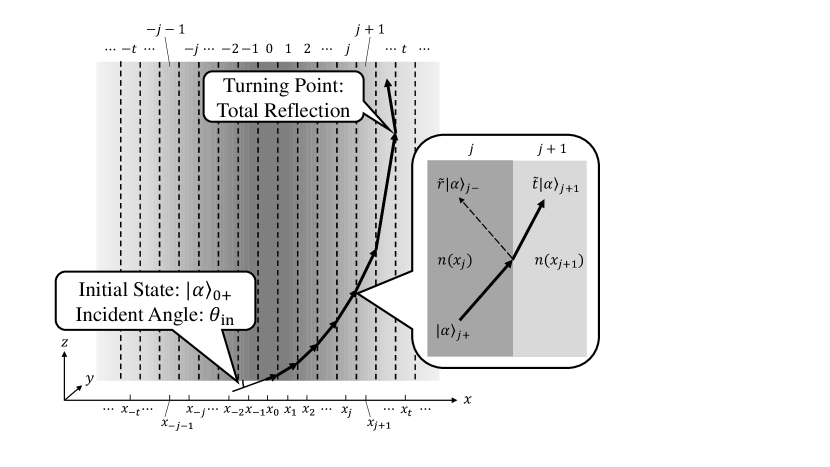
Figure 5: Graded-index slab waveguide in a symmetric structure. A power-law profile of the refractive index is considered. The core is divided into layers to represent the spatial dependence of the optical field. The optical field is supposed to enter at the $j$th layer with the incident angle $\theta_{in}$ (here, $j=0$ is indicated). The optical field travels with a trajectory.

Another interesting example is the graded-index (GI) slab waveguide. The propagation properties of GI slab waveguides have often been studied within geometric optics Snyder and Love (1983). Here we investigate it using the quantum-optical method.

A schematic of the GI slab waveguide is shown in Fig. 5. In contrast to the SI case, the refractive index of the core is dependent upon the position in the cross-section. We assume that the optical field travels in the core, without leakage to the cladding. Let us consider a power-law profile:

$$n(x)=n_{1}\sqrt{1-(g|x|)^{q}},$$ (77)

where $n_{1}$ is a refractive index at the center of the core, and $g=2\sqrt{2\Delta_{r}}/d$ is referred to as a focusing constant. The width of the core is denoted by $d$. The parameter $q$ characterizes the shape of the index distribution. Here, we study the case when $q=2$, the parabolic index waveguide that is important for optical communications .

The core is divided into layers with a common thickness $\Delta x$, similar to the SI case. In the present quantum scheme this multi-layer division enables us to take account not only of variations in refractive index, but also of the spatial dependence of the optical field. Layers are identified by the index $j$, and the center position of the $j$th layer is $x_{j}=j\Delta x$, similar to the SI case. The refractive index of the $j$th layer is represented by $n_{j}\equiv n(x_{j})$. The electromagnetic field and the state of the optical fields in the $j$th layer are denoted by $\hat{\bm{E}}_{j\pm},\hat{\bm{H}}_{j\pm}$ and $|\alpha_{j\pm}\rangle_{j\pm}$, respectively. Note here that optical fields with a wave vector consisting of positive and negative $x$-components are distinguished by the notation $j\pm$. As discussed later, the field is transmitted with no attenuation, and we can write the amplitude of the coherent state as a value independent of the spatial index $j$, that is, $\alpha_{j+}\equiv\alpha$.

Again we consider a TE mode; the state of optical field is initially in the $j$th layer at an angle $\theta_{\rm in}$ with respect to the $x$-axis. We assume that the $x$-component of the wave vector is positive and the initial state is denoted by $|\alpha\rangle_{j+}$. Let the wave vector in the $j$th layer be $\bm{k}_{j\pm}=\kappa_{j}\bm{e}_{x}\pm\beta\bm{e}_{z}$. The corresponding electromagnetic fields are represented by

$$\hat{\bm{E}}_{j\pm} = -i\sqrt{\frac{\hbar\omega}{2\varepsilon_{0}V_{j}}}[U_{tz}^{\ast}\hat{a}_{j\pm}^{\dagger}\exp(\mp i\kappa_{j}x)$$ (78a)

$$\hskip 14.22636pt-U_{tz}\hat{a}_{j\pm}\exp(\pm i\kappa_{j}x)]\bm{e}_{y},$$

$$\hat{\bm{H}}_{j\pm} = -\frac{i}{\mu_{0}}\sqrt{\frac{\hbar}{2\omega\varepsilon_{0}V_{j}}}[U_{tz}^{\ast}\hat{a}_{j\pm}^{\dagger}\exp(\mp i\kappa_{j}x)$$ (78b)

$$\hskip 14.22636pt-U_{tz}\hat{a}_{j\pm}\exp(\pm i\kappa_{j}x)](-\beta\bm{e}_{x}\pm\kappa\bm{e}_{z})$$

with double-sign in same order. Classical electromagnetic fields correspond to expectation values when in a coherent state.

States of optical fields in adjacent layers are related to each other by normalized Fresnel coefficients. Initial state $|\alpha\rangle_{j+}$ enters the interface between the $j$th and $(j+1)$th layers. After passing the interface, the state of the optical field becomes

$$\hat{\mathcal{U}}_{j,(j+1)}|\alpha\rangle_{j+}|0\rangle_{(j+1)-}=|\tilde{t}_{j,(j+1)}\alpha\rangle_{(j+1)+}|-\tilde{r}_{j,(j+1)}\alpha\rangle_{j-},$$ (79)

where

$$\hat{\mathcal{U}}_{j,(j+1)}=\exp[\vartheta_{j,(j+1)}(\hat{a}_{j+}^{\dagger}\hat{a}_{(j+1)-}-\hat{a}_{j+}\hat{a}_{(j+1)-}^{\dagger})]$$ (80)

is a unitary operator and $\tan\vartheta_{j,(j+1)}=\tilde{r}_{j,(j+1)}/\tilde{t}_{j,(j+1)}$ (see Appendix B). We find that reflection disappears at the refractive index limit, varying continuously because

$$\tilde{r}_{j,(j+1)}\propto\kappa_{j}-\kappa_{j+1}=\frac{n_{1}^{2}k_{0}^{2}g^{2}(2j+1)}{2\sqrt{n_{1}^{2}k_{0}^{2}-\beta^{2}}}\Delta x^{2}\rightarrow 0$$ (81)

as $\Delta x\rightarrow 0$. Here an approximation

$$\kappa_{j}\simeq\sqrt{n_{1}^{2}k_{0}^{2}-\beta^{2}}\left[1-\frac{n_{1}^{2}k_{0}^{2}g^{2}}{2(n_{1}^{2}k_{0}^{2}-\beta^{2})}x_{j}^{2}\right]$$ (82)

is considered. It means that the reflection of the optical field is negligible. Thus the optical field is totally transmitted with a refraction: $|\alpha\rangle_{j+}\rightarrow|\alpha\rangle_{(j+1)+}$. Similar procedures are repeated at the subsequent interfaces. The transmitted field travels according to Snell’s law.

The optical field is totally reflected when the incident angle becomes larger than the critical angle $\theta_{c}$. This point is referred to as the turning point Snyder and Love (1983). We assume that total reflection occurs when the optical field enters the layer where $j=t$: $|\alpha\rangle_{t+}\rightarrow|\alpha\rangle_{t-}$. Calculating expectation values of Eqs. (78a) and (78b) with a coherent state in each layer, we obtain electromagnetic fields that correspond to those in classical waveguide optics.

In the GI case, the optical field travels with a sinusoidal-like trajectory. This means that the optical field is not static in the cross-section, different from the SI case. An evanescent field is also generated at the turning points. However, it is small compared with the amplitude of trajectory of the optical field and is neglected here.

Figure 6: Trajectories of optical fields in the GI waveguide. Here $q=2$ is used for the power-law profile in Eq. (77). Parameters are assumed to be $\Delta x=0.1\ \mu\textrm{m}$, $n_{1}=1.45$, and $g=5.66\ \textrm{m}^{-1}$. Trajectories of initial angles $\theta_{\rm in}=84^{\circ},86^{\circ}$, and $88^{\circ}$ are drawn as sinusoidal-like curves.

As a consequence, the optical field in the GI slab waveguide travels with a periodic trajectory. In Fig. 6, trajectories of optical fields in the GI slab waveguide are shown. The initial state of the optical field is assumed to be $|\alpha\rangle_{0+}$, and the thickness of each layer $\Delta x=0.1\ \mu\textrm{m}$. Other parameters are as follows: $n_{1}=1.45$ and $g=5.66\times 10^{3}\textrm{m}^{-1}$; typical values for optical communication. Here the initial angles $\theta_{\rm in}=84^{\circ},86^{\circ}$, and $88^{\circ}$ are studied. The results show that optical fields travel with sinusoidal-like trajectories with periods in phase with each other. These quantum optics results are consistent with classical waveguide optics Snyder and Love (1983).

V Summary

We studied the propagation of an optical field in a dielectric from the perspective of quantum optics. We considered an interaction Hamiltonian between the optical field and an atom, and introduced the refractive index with the interaction Hamiltonian. We derived normalized Fresnel coefficients at an interface between different materials, and showed that they are related to the beam splitter operator. We also showed that, even for total reflection case, the evanescent field can exist outside of a reflection surface by a wavelength degree, with due consideration of the uncertainty relation.

We then studied the propagation properties of the optical fields in slab waveguides also using a viewpoint of quantum optics. A multi-layer division method was employed to represent the spatial dependence of the optical field in an inhomogeneous structure. For the step-index slab waveguide, we introduced spatially-averaged operators for static electromagnetic fields, and from them, we can evaluate the number of photons in each layer. The eigenvalue equation was derived in a similar way to classical waveguide optics. For the graded-index slab waveguide, we considered a power-law profile of the refractive index. We showed that optical fields travels with a sinusoidal-like trajectory, similar to those in classical waveguide optics.

When the coherent state shows high amplitude the results obtained here are reduced to those of classical waveguide optics. By contrast, for small amplitudes, the quantum properties of optical fields in waveguides can be determined with the present scheme.

Appendix A Derivation of Eq. (15)

The interaction Hamiltonian between optical fields and an atom in a cavity was discussed in Schneider et al. (1997). A similar procedure is valid for the present case, and we review it in the following:

We assume that the electric dipole approximation can be applied to the present model, and that the interaction Hamiltonian in the Schrödinger picture is, under the rotating wave approximation, given by

$$\hat{\mathcal{V}}=\sqrt{2}i\hbar g(\hat{A}\hat{\sigma}_{+}-\hat{A}^{\dagger}\hat{\sigma}_{-}),$$ (83)

where

$$g=\sqrt{\frac{\omega}{2\hbar\varepsilon_{0}V}}\bm{\wp}_{eg}\cdot\bm{e}$$ (84)

is the coupling constant. Here $\bm{\wp}_{eg}$ and $\bm{e}$ are the electric dipole transition matrix element and a vector parallel to polarization direction, respectively. The operator

$$\hat{A}=\frac{\hat{a}_{p}+\hat{a}_{s}}{\sqrt{2}}$$ (85)

and its Hermitian conjugate satisfy a commutation relation,

$$[\hat{A},\hat{A}^{\dagger}]=1.$$ (86)

In the interaction picture, we have

$$\hat{\mathcal{V}}_{I}(t) = \exp\left(i\frac{\hat{\mathcal{H}}_{0}}{\hbar}t\right)\hat{\mathcal{V}}\exp\left(-i\frac{\hat{\mathcal{H}}_{0}}{\hbar}t\right)$$

$$= \sqrt{2}i\hbar g\left[\hat{A}\hat{\sigma}_{+}\exp(i\Delta\omega t)-\hat{A}^{\dagger}\hat{\sigma}_{-}\exp(-i\Delta\omega t)\right].$$

The time-development operator is calculated as

$$\hat{U}_{I}(t) \simeq \hat{1}-\frac{i}{\hbar}\int_{0}^{t}dt^{\prime}\hat{\mathcal{V}}_{I}(t^{\prime})$$ (88)

$$\hskip 28.45274pt-\frac{1}{\hbar^{2}}\int_{0}^{t}dt^{\prime}\hat{\mathcal{V}}_{I}(t^{\prime})\int_{0}^{t^{\prime}}dt^{\prime\prime}\hat{\mathcal{V}}_{I}(t^{\prime\prime})$$

$$\simeq \hat{1}-2i\frac{g^{2}}{\Delta\omega}[\hat{A}\hat{\sigma}_{+},\hat{A}^{\dagger}\hat{\sigma}_{-}]t$$

$$\simeq \exp\left(-i\frac{\hat{\mathcal{H}}^{\prime}_{\rm eff}}{\hbar}t\right),$$

where

$$\hat{\mathcal{H}}^{\prime}_{\rm eff}=2\hbar\chi(\hat{\sigma}_{+}\hat{\sigma}_{-}+\hat{A}^{\dagger}\hat{A}\sigma_{z})$$ (89)

and we introduce

$$\chi=g^{2}/\Delta\omega.$$ (90)

In this calculation, the first integral is ignored as a small value under the assumption that the mean excitation $\langle\hat{A}\rangle\approx(\langle\hat{A}^{\dagger}\hat{A}\rangle)^{1/2}$ is not so large, that is,

$$\left|\frac{g}{\Delta\omega}\sqrt{\hat{A}^{\dagger}\hat{A}}\right|\ll 1,$$ (91)

and terms proportional to $(\Delta\omega)^{-2}$ and any higher order is also ignored.

The atomic state remains in the ground state $|g\rangle_{a}$ before and after the interaction, and we calculate the expectation value of Eq. (89) with respect to the atomic state.

$${}_{a}\langle g|\hat{\mathcal{H}}_{\rm eff}^{\prime}|g\rangle_{a} = -\hbar\chi(\hat{a}_{p}\hat{a}_{s}^{\dagger}+\hat{a}_{p}^{\dagger}\hat{a}_{s}$$ (92)

$$\hskip 28.45274pt+\hat{a}_{p}^{\dagger}\hat{a}_{p}+\hat{a}_{s}^{\dagger}\hat{a}_{s}),$$

taking Eqs. (10a), (10b), (85), and $\sigma_{-}|g\rangle_{a}=0$ into account. Since the third and fourth terms on the right hand side of Eq. (92) are adequately small compared with the free Hamiltonian (6) and they can be ignored, then we obtain the effective interaction Hamiltonian (15).

Assuming that the optical fields and atom interact during $\Delta\tau$, we have the time evolution from the initial state to the final one,

$${}_{a}\langle g|\hat{U}_{I}(\Delta\tau)|g\rangle_{a}=\exp\left(-i\frac{\hat{\mathcal{H}}_{\rm eff}}{\hbar}\Delta\tau\right),$$ (93)

which appears in Eq. (16).

Appendix B Beam splitter operator

We introduce a unitary operator:

$$\hat{\mathcal{U}}_{jj^{\prime}}=\exp[i\vartheta(\hat{a}_{j}\hat{a}_{j^{\prime}}^{\dagger}+\hat{a}_{j}^{\dagger}\hat{a}_{j^{\prime}})],$$ (94)

where $\vartheta$ is a real parameter. Using this operator, we find that operators $\hat{a}_{j}$ and $\hat{a}_{j^{\prime}}$ are transformed into Barnett and Radmore (1997)

$$\hat{\mathcal{U}}_{jj^{\prime}}\hat{a}_{j}\hat{\mathcal{U}}_{jj^{\prime}}^{\dagger} = \hat{a}_{j}\cos\vartheta-i\hat{a}_{j^{\prime}}\sin\vartheta,$$ (95)

$$\hat{\mathcal{U}}_{jj^{\prime}}\hat{a}_{j^{\prime}}\hat{\mathcal{U}}_{jj^{\prime}}^{\dagger} = -i\hat{a}_{j}\sin\vartheta+\hat{a}_{j^{\prime}}\cos\vartheta.$$ (96)

Two coherent states $|\alpha\rangle_{j}$ and $|\alpha^{\prime}\rangle_{j^{\prime}}$ are combined by multiplying them by the operator (94) because

$$\hat{\mathcal{U}}_{jj^{\prime}}|\alpha\rangle_{j}|\alpha^{\prime}\rangle_{j^{\prime}}$$ (97)

$$= \hat{\mathcal{U}}_{jj^{\prime}}\hat{D}_{j}(\alpha)\hat{\mathcal{U}}_{jj^{\prime}}^{\dagger}\hat{\mathcal{U}}_{jj^{\prime}}\hat{D}_{j^{\prime}}(\alpha^{\prime})\hat{\mathcal{U}}_{jj^{\prime}}^{\dagger}|0\rangle$$

$$= \hat{D}_{j}(\alpha\cos\vartheta)\hat{D}_{j}(i\alpha^{\prime}\sin\vartheta)$$

$$\hskip 28.45274pt\times\hat{D}_{j^{\prime}}(i\alpha\sin\vartheta)\hat{D}_{j^{\prime}}(\alpha^{\prime}\cos\vartheta)|0\rangle$$

$$= \hat{D}_{j}(\alpha\cos\vartheta+i\alpha^{\prime}\sin\vartheta)$$

$$\hskip 28.45274pt\times\hat{D}_{j^{\prime}}(i\alpha\sin\vartheta+\alpha^{\prime}\cos\vartheta)|0\rangle$$

$$= |\alpha\cos\vartheta+i\alpha^{\prime}\sin\vartheta\rangle_{j}|i\alpha\sin\vartheta+\alpha^{\prime}\cos\vartheta\rangle_{j^{\prime}},$$

where $\hat{D}_{j}(\alpha)=\exp(\alpha\hat{a}_{j}^{\dagger}-\alpha^{\ast}\hat{a}_{j})$ is the displacement operator, and the relations (95), (96) and their Hermitian conjugates are considered. Here, the Baker-Hausdorff formula Louisell (1973) and $\hat{\mathcal{U}}_{jj^{\prime}}|0\rangle=|0\rangle$ are also considered.

By replacing $\hat{a}_{j^{\prime}}$ with $-i\hat{a}_{j^{\prime}}$, we obtain another unitary operator:

$$\hat{\mathcal{U}}^{\prime}_{jj^{\prime}}=\exp[\vartheta(\hat{a}_{j}^{\dagger}\hat{a}_{j^{\prime}}-\hat{a}_{j}\hat{a}_{j^{\prime}}^{\dagger})].$$ (98)

The annihilation operators and coherent states are similarly transformed into

$$\hat{\mathcal{U}}^{\prime}_{jj^{\prime}}\hat{a}_{j}\hat{\mathcal{U}}^{\prime\dagger}_{jj^{\prime}} = \hat{a}_{j}\cos\vartheta-\hat{a}_{j^{\prime}}\sin\vartheta,$$ (99)

$$\hat{\mathcal{U}}^{\prime}_{jj^{\prime}}\hat{a}_{j^{\prime}}\hat{\mathcal{U}}^{\prime\dagger}_{jj^{\prime}} = \hat{a}_{j}\sin\vartheta+\hat{a}_{j^{\prime}}\cos\vartheta.$$ (100)

$$\hat{\mathcal{U}}^{\prime}_{jj^{\prime}}|\alpha\rangle_{j}|\alpha^{\prime}\rangle_{j^{\prime}} = |\alpha\cos\vartheta+\alpha^{\prime}\sin\vartheta\rangle_{j}$$ (101)

$$\hskip 14.22636pt\otimes|-\alpha\sin\vartheta+\alpha^{\prime}\cos\vartheta\rangle_{j^{\prime}}$$

with the operator (98).

We can see from Eqs. (97) or (101) that the optical fields of modes $j$ and $j^{\prime}$ are combined with $\hat{\mathcal{U}}_{jj^{\prime}}$ or $\hat{\mathcal{U}}^{\prime}_{jj^{\prime}}$. These operations physically correspond to a beam splitter.

Appendix C Derivation of Eqs. (70) and (76)

Here we derive relations betweeng eigenvalues of coherent states in areas (I), (II), and (III), and the eigenvalue equation from the continuity condition of the electromagnetic fields. Note that optical fields are totally reflected at interfaces between (I)-(II) and (II)-(III) and that there are evanescent fields in areas (I) and (III) in the step-index guiding case. The $x$-component of Poynting vector is calculated as a pure imaginary number, and it is not observable quantity. This means that energy flow from the core to cladding does not exist. Thus, normalization of the electromagnetic fields such as in Eq. (30) is not necessary.

For the TE even mode, for example, continuity conditions of the electromagnetic fields are

$$\alpha^{\rm(I)}\exp\left(-\frac{\gamma d}{2}\right) = \sqrt{2}\alpha^{\rm(II)}_{\rm even}\cos\frac{\kappa d}{2}$$ (102a)

$$= \alpha^{\rm(III)}\exp\left(-\frac{\gamma d}{2}\right),$$

$$\gamma\alpha^{\rm(I)}\exp\left(-\frac{\gamma d}{2}\right) = \sqrt{2}\kappa\alpha^{\rm(II)}_{\rm even}\sin\frac{\kappa d}{2}$$ (102b)

$$= \gamma\alpha^{\rm(III)}\exp\left(-\frac{\gamma d}{2}\right).$$

From Eq. (102a), eigenvalues are related as in Eq. (70a). The condition (102) is, in a matrix form, reduced to

$$\left(\begin{array}[]{cc}\exp\left(-\frac{\gamma d}{2}\right)&-\sqrt{2}\cos\frac{\kappa d}{2}\\ \gamma\exp\left(-\frac{\gamma d}{2}\right)&-\sqrt{2}\kappa\sin\frac{\kappa d}{2}\end{array}\right)\left(\begin{array}[]{c}\alpha^{\rm(I)}\\ \alpha^{\rm(II)}_{\rm even}\end{array}\right)=0.$$ (103)

For a non-trivial solution, the determinant of the coefficient matrix should be zero, and we obtain the eigenvalue equation for the TE even mode in Eq. (76). A similar procedure is applicable for the TE odd mode.

References

- Snitzer (1961) E. Snitzer, J. Opt. Soc. Am. 51, 491 (1961).
- Snyder and Love (1983) A. W. Snyder and J. D. Love, Optical Waveguide Theory (Chapman and Hall, 1983).
- Nielsen and Chuang (2000) M. A. Nielsen and I. L. Chuang, Quantum Computation and Quantum Information (Cambridge, 2000).
- Braunstein and Pati (2003) S. L. Braunstein and A. K. Pati, Quantum Information with Continuous Variables (Kluwer, 2003).
- Gisin and Thew (2007) N. Gisin and R. Thew, Nature Photonics 1, 165 (2007).
- Sasaki et al. (2011) M. Sasaki et al., Opt. Express 19, 10387 (2011).
- Feynman et al. (1965) R. P. Feynman, R. B. Leighton, and M. L. Sands, The Feynman Lectures on Physics Vol. I (Addison Wesley, 1965).
- Hecht (2001) E. Hecht, Optics, 4th ed. (Addison-Wesley, 2001).
- Drummond and Corney (2001) P. D. Drummond and J. F. Corney, J. Opt. Soc. Am. B 18, 139 (2001).
- Hecht (1973) E. Hecht, Am. J. Phys. 41, 1008 (1973).
- Zia (1988) R. K. P. Zia, Am. J. Phys. 56, 555 (1988).
- Barnett and Radmore (1997) S. M. Barnett and P. M. Radmore, Methods in Theoretical Quantum Optics (Oxford, 1997).
- Gerry and Knight (2005) C. C. Gerry and P. L. Knight, Introductory Quantum Optics (Cambridge, 2005).
- Louisell (1973) W. H. Louisell, Quantum Statistical Properties of Radiation (Wiley, 1973).
- Born and Wolf (1999) M. Born and E. Wolf, Principle of Optics, 7th Ed. (Cambridge, 1999).
- Note (1) This formulation was also referred to in an unpublished work by M. Matsuoka.
- Navasquillo et al. (1989) J. Navasquillo, V. Such, and F. Pomer, Am. J. Phys. 57, 1109 (1989).
- Lodenquai (1991) J. F. Lodenquai, Am. J. Phys. 59, 248 (1991).
- Note (2) The optimum distribution of the refractive index is known as . It was particularly discussed in the following article: S. Kawakami and J. Nishizawa, IEEE Trans. Microwave Theory Tech., MTT-16, 814 (1968).
- Schneider et al. (1997) S. Schneider, A. M. Herkommer, U. Leonhardt, and W. P. Schleich, J. Mod. Opt. 44, 2333 (1997).