Nonlinear Conductivity in Graphene

Abstract

We consider the tight-binding approximation for the description of energy bands of graphene, together with the standard Boltzmann s transport equation and constant relaxation time, an expression for the conductivity was obtained. We predicted strong nonlinear effects in graphene which may be useful for high frequency generation.
Keywords: Graphene, Mathematical model, Nonlinear effects, High Frequency Radiation.

1 Introduction

Graphene was discovered by Novoselov et al in 2004 [1]- [3] and has since attracted a great deal of interest due to its unique properties like mechanical, electrical, thermal, etc arising from its highly symmetric two-dimensional honeycomb-lattice structure [4, 5]. This makes graphene potentially applicable in carbon-based nanoelectronics‘[6, 7]. The nonquadratic energy spectrum of graphene allows it to exhibit nonlinear phenomena [8] and its non-addivity property provides the mutual dependence of electron or hole motion in orthogonal directions [9]. Several unique physical properties of graphene have been studied both theoretically and experimentally [8]- [12].

Investigation into electronic properties of graphene has revealed that the electron dispersion law is linear in momemtum near the Fermi points and thereby causing the quasiparticles to behave like massless Dirac Fermions [12]. However, the tendency of graphene to absorb impurities on its surface and interacts with the impurities electrons results in the formation of nonparabolicity of the energy band which makes the electronic properties of graphene essentially nonlinear under moderate electric fields [13]. This nonlinearity makes graphene to exhibit plethora of transport phenomena [12]- [20]. Under different conditions of an external electric field, an electron in graphene is predicted to reveal a variety of physical effects such as Bloch oscillations, self-induced transparency, absolute negative conductance, etc. Electronic properties and electronic transport in graphene is the subject of many theoretical papers [12]- [20]. Nevertheless, the electrodynamic properties of graphene is worth further studying because it is the basis for developing carbon-based devices. Using the kinetic transport equation, we shall in this work study the effect of high frequency (hf) conductivity in graphene by following the approaches of [21]- [26].

2 Theory

Proceeding as in references [21]- [26], we consider the motion of an electron in the presence of high frequency electric field $E(t)$. The electric field $E(t)$ is directed along the graphene axis and the conductivity is derived using the Boltzmann kinetic equations describing electron transport in graphene for the distribution functions in the relaxation time approximation as follows:

$$\frac{\partial f_{s}}{\partial t}+eE(t)\frac{\partial f_{a}}{\partial\mathbf{p}}=\frac{F-f_{s}}{\tau}$$ (1)

$$\frac{\partial f_{a}}{\partial t}+eE(t)\frac{\partial f_{s}}{\partial\mathbf{p}}=\frac{-f_{a}}{\tau}$$ (2)

where $e$ is the electron charge, $\mathbf{p}$ is the electron dynamical momentum, $F$ is the equilibrium distribution function and $f_{s}$ as well as $f_{a}$ the symmetric and antisymmetric distribution functions respectively. Solving Eqs.($1$) and ($2$) in a constant electric field yields,

$$\frac{\partial^{2}f_{a}^{o}}{\partial\xi^{2}}-\chi_{o}^{2}f_{a}^{o}=\frac{\partial F}{(eEa\tau)\partial\xi}$$ (3)

where $\xi_{o}^{2}=\frac{\pi^{2}}{(eEa\tau)^{2}}$ and $\mathbf{p}=\frac{\pi}{a}\xi$.See [26]
Using $\frac{\partial F}{\partial\xi}=\frac{\partial F}{\partial\varepsilon}\frac{\partial\varepsilon}{\partial\xi}$, the solution to Eq.($2$) for the necessary boundary conditions $f_{a}(-1)=f_{a}(+1)=0$ is

$$f^{o}_{a}=\varepsilon\frac{\partial F}{\partial\varepsilon}\frac{eaE\tau}{(eaE\tau)^{2}+1}$$ (4)

The spectrum of electrons in graphene is given by [24,25].

$$|\varepsilon(p)|=\pm\frac{3\gamma_{o}b}{2\hbar}|\mathbf{p}-\mathbf{p_{F}}|$$ (5)

where $\gamma_{0}\approx 2.7eV$,$b=0.142nm$ is the distance between the neighbouring carbon atoms in the graphene. $+$ and $-$ signs are related to the conduction and valence bands respectively. With $p_{F}$ as the constant quasimomentum corresponding to the particular Fermi point. The current density of the mobile electron in the $1^{st}$ Bz for graphene is given as [24, 25]

$$j_{x}=\frac{2e}{(2\pi\hbar)^{2}}\int\int v_{x}f_{a}^{o}d^{2}\mathbf{p}$$ (6)

and the quasiclassical velocity $v_{x}(p)$ of an electron moving along the graphene axis can be

$$v_{x}(p)=\frac{\partial\varepsilon}{\partial p}=\frac{a}{\pi}\frac{\partial\varepsilon}{\partial\xi}=\frac{a}{\pi}grad\varepsilon$$ (7)

and writing

$$d^{2}\mathbf{p}=\frac{\pi}{a}d^{2}\xi=\frac{\pi}{a}\frac{ds}{|\frac{a}{\pi}grad\varepsilon|}dE$$ (8)

$ds$ is the element of the length of the curve.
Substituting Eqs.($3$),($6$) and($7$) into($5$) we get,

$$j_{x}=-\frac{e^{2}}{2\pi(\hbar)^{2}}\frac{E\tau}{(eaE\tau)^{2}+1}\int|\varepsilon|\frac{\partial F}{\partial\varepsilon}d\varepsilon$$ (9)

Using (4), we obtain

$$j_{x}=\frac{8ln2}{\pi(\hbar)^{2}}\frac{\tau e^{2}k_{B}TE}{(\omega_{B}\tau)^{2}+1}$$ (10)

and

$$\sigma_{x}=\frac{8ln2}{\pi(\hbar)^{2}}\frac{\tau e^{2}k_{B}T}{(\omega_{B}\tau)^{2}+1}$$ (11)

where $\omega_{B}\tau=eaE\tau$. See![26]
By linearizing Eqs. ($1$) for the perturbation

$$E(t)=(E+E_{\omega,k}e^{-i(\omega t+kx)}),f_{s}=f_{s}^{o}+f_{s}^{1}e^{-i(\omega t+kx)},f_{a}=f_{a}^{1}e^{-i(\omega t+kx)}$$ (12)

we obtain

$$\frac{\partial^{2}f_{a}^{1}}{\partial\xi^{2}}-\chi_{\omega}^{2}f_{a}^{1}=\pi^{2}\frac{(i\omega\tau-1)}{(eaE\tau)^{2}}f_{a}^{o}\frac{E_{\omega k}}{E}-\frac{\partial^{2}f_{a}^{o}}{\partial\xi^{2}}\frac{E_{\omega k}}{E}$$ (13)

where

$$\chi_{\omega}^{2}=\frac{\{1-2i\omega\tau-(\omega\tau)^{2}\}}{(eaE\tau)^{2}}$$ (14)

Using $\frac{\partial F}{\partial\xi}=\frac{\partial F}{\partial\varepsilon}\frac{\partial\varepsilon}{\partial\xi}$, the solution to Eq(11) for the necessary boundary conditions $f_{a}(-1)=f_{a}(+1)=0$ is

$$f_{a}^{1}=\left[\varepsilon\frac{\partial F}{\partial\varepsilon}\left(\frac{(eaE\tau)}{(eaE\tau)^{2}+1}\right)\frac{E_{\omega k}}{E}\left\{\frac{i\omega\tau-1-(eaE\tau)^{2}}{(eaE\tau)^{2}-(\omega\tau)^{2}+1-2i\omega\tau}\right\}\right]$$ (15)

Substituting Eqs.($12$),($6$)and($7$) into($5$) and using ($4$), we obtain we get,

$$j_{x}=-\frac{e^{2}}{2\pi(\hbar)^{2}}\left(\frac{(eaE\tau)}{(eaE\tau)^{2}+1}\right)\left\{\frac{i\omega\tau-1-(eaE\tau)^{2}}{(eaE\tau)^{2}-(\omega\tau)^{2}+1-2i\omega\tau}\right\}$$

$$\times\int|\varepsilon|\frac{\partial F}{\partial\varepsilon}d\varepsilon$$ (16)

where $\int|\varepsilon|\frac{\partial F}{\partial\varepsilon}d\varepsilon=K_{\beta}Tln2$ making Eqn.($16$) yield

$$j_{x}=-\frac{K_{\beta}Tln2e^{2}}{2\pi(\hbar)^{2}}\left(\frac{(eaE\tau)}{(eaE\tau)^{2}+1}\right)\left\{\frac{i\omega\tau-1-(eaE\tau)^{2}}{(eaE\tau)^{2}-(\omega\tau)^{2}+1-2i\omega\tau}\right\}$$

$$\sigma_{x}(\omega)=\sigma_{o}\left\{\frac{i\omega\tau-1-(eaE\tau)^{2}}{(\omega_{B}\tau)^{2}-(\omega\tau)^{2}+1-2i\omega\tau}\right\}$$ (18)

where $eaE\tau=\omega_{B}\tau$ and $\sigma_{o}=\frac{2ln2\tau e^{2}k_{B}T}{\pi(\hbar)^{2}}\frac{\omega_{B}\tau}{(\omega_{B}\tau)^{2}+1}$. See [26]

3 Results, Discussion and Conclusion

We present the results of a kinetic equation approach of a graphene subject to constant electric field $E$. The electric field $E$ is directed along the graphene axis. Exact expression for the direct conductivity was obtained in eq.(9). The nonlinearity is analyzed using the dependence of the normalized conductivity $j_{x}$ as a function of $E$. . Figure 1 illustrates the dependence of $j_{x}$ on $E$. The figure shows a linear dependence of $j_{x}$ on $E$ at weak values of $E$. As E increases, $j_{x}$ increases, and at a some value of $E$, $j_{x}$ reaches a maximum value. Further increase in $E$ results in the decrease of $j_{x}$. The slope of the curve is the dc differential conductivity, $\sigma_{x}=dj_{x}/dE$. See equation (10). If $E\approx 1$, the Bloch frequency is in the terahertz frequency range and if $E>1$, $\sigma_{x}$ is negative and therefore graphene demonstrates negative differential conductivity (NDC). Figure 2 elucidates the graph of conductivity component $(\sigma_{x}(\omega))/\sigma_{o}$ obtained in Eq. (14) on the normalized frequency $\omega/\omega_{B}$ . The dimensionless complex conductivity $(\sigma_{x}ω)/\sigma_{o}$ depends strongly and nonlinearly on the normalized frequency $\sigma/\omega_{B}$ . We observed that the real part of the complex conductivity will become more negative with increasing frequency, until a resonance minimum occurs just before the Bloch frequency $\omega_{B}\tau$. This negative-conductivity resonance close to the Bloch frequency makes the graphene an active medium for a Bloch oscillator without domain instabilities induced by negative dc conductivity. In summary, using the solution of the Boltzmann’s transport equation with constant relaxation time $\tau$ approximation, we obtained an exact expression for the conductivity of graphene. We noted a strong nonlinear effets which may be useful for the generation of high frequemcy radiation.

Figure 1: A plot of current density $j_{x}$ as a function of $E$ in graphene for expression ($9$).

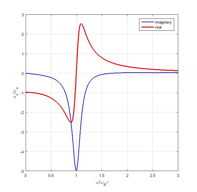
Figure 2: A plot of a normalized complex conductivity ($\sigma_{x}\omega)/\sigma_{0}$ as a function of dimensionless frequency $\omega/\omega_{\beta}$ in graphene for expression ($9$) when $\omega_{\beta}\tau=10$.

References

- [1] Novoselov, K. S., Geim, A. K., Morozov, S. V., Jiang, D., Zhang, Y, Dubonos, S. V., Grigorieva, I. V. and Firsov, A. A., Electric field effect in atomically thin carbon films, Science 306: 666 669 5 (2004).
- [2] Novoselov, K. S., Geim, A. K., Morozov, S. V., Jiang, D., Katsnelson, M. I., Grigorieva, I. V., Dubonos, S. V. and Firsov, A. A., Two-dimensional gas of massless Dirac fermions in graphene, Nature438: 197 200 (2005).
- [3] Zhang, Y., Tan, Y.-W., Stormer, H. L. and Kim, P., Experimental observati on of the quantum Hall effect and Berry s phase in graphene, Nature 438: 201 204 (2005).
- [4] Neto, A. H.C., Guinea, F., Peres, N. M. R., Novoselov, K. S., and Geim, A. K., The electronic properties of graphene, Rev. Mod. Phys. 81: 109 162 (2009).
- [5] Katsnelson, M. I., Graphene: carbon in two dimensions, Materials Today 10: 20 27 (2007).
- [6] Geim, A. K., Graphene: Status and prospects, Science 324: 1530 1534. (2009).
- [7] Stankovich, S., Dikin, D. A., Dommett, G. H. B., Kohlhaas, K. M., Zimney, E. J., Stach, E. A., Piner, R. D., Nguyen, S. T., and Ruoff, R. S., Graphene-based composite materials. Nature 442 282 6 (2006).
- [8] Katsnelson, M. I., Minimal conductivity in bilayer graphene, Europ. Phys. J. B 52: 151 153 (2006).
- [9] Nomura, K. and MacDonald, A. H., Quantum transport of massless Dirac fermions, Phys. Rev. Lett. 98: 076602 (2007)
- [10] Tan, Y.-W., Zhang, Y., Bolotin, K., Zhao, Y., Adam, S., Hwang, E. H., Das Sarma, S., Stormer, H. L. and Kim, P. Measurement of scattering rate and minimum conductivity in graphene, Phys. Rev. Lett. 99: 246803, (2007).
- [11] Young, A. F. and Kim, P., Quantum interference and Klein tunnelling in graphene heterojunctions, Nature Physics 5: 222 226 (2009).
- [12] Belonenko, M. B., Lebedev, N. G., and Tuzalina, O. Yu., Electromagnetic Solitons in a System of Graphene Planes with Anderson Impurities, Journal of Russian Laser Research, Vol. 30, No. 2, 2009, pp. 102-109
- [13] Mikhailov, S. A., Non-linear electromagnetic response of graphene, Europhys. Lett. 79: 27002 (2007).
- [14] Mikhailov, S. A., Electromagnetic response of electrons in graphene: Nonlinear effects, Physica E 40: 2626 2629(2008).
- [15] Mikhailov, S. A. Non-linear graphene optics for terahertz app lications, Microelectron. J. 40: 712 715 (2009).
- [16] Mikhailov, S. A. and Ziegler, K. New electromagnetic mode in graphene, Phys.Rev.Lett. 99: 016803 (2007).
- [17] Mikhailov, S. A. and Ziegler, K., Non-linear electromagnetic response of graphene: Frequency multiplication and the self-consistent field effects, J. Phys. Condens. Matter 20: 384204 (2008).
- [18] Zav yalov, D. V., Kryuchkov, S. V., and Marchuk, . V., On the possibility of transverse current rectification in graphene, Technical Physics Letters, 34(11), 915 (2008).
- [19] Zav yalov, D. V., Kryuchkov, S. V., and Tyulkina, T. A., Effect of rectification of current induced by an electromagnetic wave in graphene: A numerical simulation, Semiconductors, 44(7), 879 (2010).
- [20] Kryuchkov , S. V., Kuhar, E. I. and Yakovenko, V. A., Effect of mutual rectification rectification of two electromagnetic waves with perpendicular polarization planes in a superlattice based on graphene, Bulletin of the Russian Academy of Sciences: Physics V. 74 ? 12 2010 P. 1679-1681.
- [21] Bass, F. G., Bulgakov, A. A., and Tetervov, A. P., High-Frequency Properties of Semiconductors with Superlattices (Nova Science, New York, 1997)
- [22] Shmelev, G M, Epshtein, E M and Belonenko, M. B., Current oscillations in a superlattice under non-quantizing electric and magnetic fields arXiv: 0905.3457v2 (2009).
- [23] Ignatov, A. A., Schomburg, E., Grenzer, J., Renk, K. F., and Dodin, E. P., THz-field induced nonlinear transport and dc voltage generation in a semiconductor superlattice due to Bloch oscillations, Z. Physik B , vol. 98, pp. 187-195, 1995
- [24] Wallace, P. R., The band theory of graphite , Phys. Rev. 71 622 34 (1947)
- [25] Slepyan, G. Ya., Maksimenko, S. A., Lakhtakia, A., Yevtushenko, O. and Gusakov, A. V., Electrodynamics of carbon nanotubes: Dynamic conductivity, impedance boundary conditions,and surface wave propagation , Phy. Rev. B 60, 24 (1999).
- [26] Ktitorov, S. A., G. S. Simin, Sindalovskii, V. Ya. Bragg reflections and the high-frequency conductivity of an electronic solid-state plasma , Sov. Phys. Sol. State 13, 1872 (1972)