Generalized Transformation Design: metrics, speeds, and diffusion

Abstract

We show that a unified and maximally generalized approach to spatial transformation design is possible, one that encompasses all second order waves, rays, and diffusion processes in anisotropic media. Until the final step, it is unnecessary to specify the physical process for which a specific transformation design is to be implemented. The principal approximation is the neglect of wave impedance, an attribute that plays no role in ray propagation, and is therefore irrelevant for pure ray devices; another constraint is that for waves the spatial variation in material parameters needs to be sufficiently small compared with the wavelength. The key link between our general formulation and a specific implementation is how the spatial metric relates to the speed of disturbance in a given medium, whether it is electromagnetic, acoustic, or diffusive. Notably, we show that our generalised ray theory, in allowing for anisotropic indexes (speeds), generates the same predictions as does a wave theory, and the results are closely related to those for diffusion processes.

I Introduction

Transformation design (T-Design) is a way of constructing devices based directly on a mathematical specification. The essence of the idea is that it lets us shift waves, rays, or other excitations around inside the device, while altering the way they propagate, so that the outside world sees no changes. Here we make this more mathematically precise through a two stage process: first by defining a "morphism" picture that applies equally to all cases, and then a second step that matches the morphism picture to the specific physical system.

The most notable example of T-Design is that of electromagnetic cloaking, which has now been with us for almost ten years Pendry et al. (2006); Leonhardt (2006). It has been recently revitalized by the introduction of the concept of space-time cloaking McCall et al. (2011); Kinsler and McCall (2014a); Gratus et al. (2016) and its variety of implementations Fridman et al. (2012); Lukens et al. (2014); Chremmos (2014); Jabar et al. (2015) In light of the many variants of spatial cloaking, and of applications in acoustics Zhang et al. (2011); Sanchis et al. (2013) and diffusion of heat or light Guenneau et al. (2012); Schittny et al. (2015), it is worth considering how to combine these different applications and approaches into a unified T-Design scheme, at least to the extent possible. Some progress has been made in that regard, but with a firm focus on wave mechanics expressed in a first-order form Kinsler and McCall (2014b).

Here we take an exclusively second order approach in which a subset of variables satisfying a system of first order equations are expressed as a single second order equation. For example, instead of examining transformations of Maxwell’s equations in the field vectors $\textbf{E},\textbf{B},\textbf{D}$ and H, we will consider just the simplest (Helmholtz-like) second order wave equation a single field component, e.g. just $E$, or just $B$. Although less detailed than first-order approaches, notably in the way impedance is ignored, the second-order approach has some significant advantages. In any case, when it comes to actual Transformation devices (T-devices) – often impedances are ruthlessly ignored or rescaled to suit the technological demands of the programme. In that sense including impedance could be considered somewhat over careful. T-devices in which no attempt is made to control scattering or reflections from impedance mismatches have a performance left hostage to the physics of the wave or ray they attempt to manipulate. Notably, we expect that in principle electromagnetic (EM) T-devices are less imperfect than acoustic ones Kinsler and McCall (2014b).

We start by taking a second order wave equation as describing a given system, and see how it can be modified to allow for anisotropy. Since, largely, any wave type can be modelled this way, this is not a particularly stringent restriction. We then show how the equation can be recast into a covariant form, where the covariant derivative is that associated with the space’s underlying metric, $g_{\alpha\beta}$. Transformation design is then described as a mathematical morphism between a reference or “design” solution and a T-device application; the extraction of material parameters from the morphed/transformed metric – for whatever physical system is of interest – is then solely a problem of calculation.

In section II we present the basic wave, ray, and diffusion machinery in the context of our second-order approach, and how, for a given choice of physical system, the material properties map onto the effective metric. In section III we show how the metric morphs under transformation, and in section IV we give examples. Finally, in section V we summarize our results.

II Waves, Rays, and Diffusions

In what follows we will generalise the common second order wave equation approach for T-Design to allow for anisotropy of the propagation in the simplest possible way. We then demonstrate how this generalization allows a unified process for designing T-devices for almost any sort of wave, ray, or diffusion. This is because all these types of processes can have their mathematical expression and behaviour mapped on to the metric seen by the process, so that a transformation of a metric is sufficent to determine the necessary material parameters for the chosen T-device.

II.1 Waves

The most general type of second order wave model is given by the covariant wave equation on a manifold where the spatial part of the metric ${g}\indices{{}_{ij}}$ has its inverse counterpart ${g}\indices{{}^{ij}}$. In indexed notation using the Einstein summation convention, with Greek indices spanning $\{t,x,y,x\}$ and Latin ones spanning $\{x,y,z\}$, and treating the time coordinate $t$ separately from space, this is

$$\Psi\indices{{}^{;\mu}_{;\mu}}=\operatorname{\nabla}_{i}\left({g}\indices{{}^{ij}}\operatorname{\nabla}_{j}\Psi\right)+{g}\indices{{}^{tt}}\partial_{t}^{2}\Psi =0,$$ (1)

where $g\indices{{}^{\mu\nu}}$ is inverse to $g\indices{{}_{\mu\nu}}$. The separation between space and time is justified when we are only interested in spatial morphisms. Here both “$;\mu$” and $\operatorname{\nabla}_{\mu}$ denote covariant derivatives, whereas $\partial_{\mu}$ are partial derivatives. This equation is for a scalar field $\Psi$, but the generalization to other types of waves is straightforward. Note that for wave processes, we have ${g}_{tt}={g}^{tt}=-1$.

Equation (1) can be compared to the standard wave equation for a field in a homogeneous isotropic medium (e.g. consider light travelling in an ordinary block of glass).

$$\left[\sum_{i}\partial_{i}\left(v^{2}\partial_{i}\right)-\partial_{t}^{2}\right]\Psi(\textbf{r},t) =0.$$ (2)

This non-covariant form of the second order wave equation is posed in Euclidean coordinates in which there is no need to distinguish between co-variant and contra-variant indices. Placing the homogeneous $v^{2}$ wave property between the two spatial derivatives facilitates comparison with the covariant form of (1). The use of a squared property is also worthy of note – it has also been argued that for electromagnetic waves in media, the refractive index squared is a much more relevant quantity than index $n$ in optical propagation Kinsler (2009), in particular as to how it affects the best definition of wavevector in the presence of significant gain or loss.

Comparing (1) and (2) we see that they have a very similar form – the difference being that the isotropic and scalar speed squared ($v^{2}$) has been replaced by the potentially anisotropic inverse spatial metric ${g}\indices{{}^{ij}}$. Thus the somewhat abstract notion of the inverse of the metric on a manifold can be replaced by the concrete and intuitive notion of a speed (squared) matrix (which we will denote using the Fraktur ‘C’ character as ${\mathfrak{C}}^{ij}$).

Allowing anisotropy by considering materials with a speed matrix ${\mathfrak{C}}^{ij}$ rather than an isotropic $v^{2}$ is crucial for the field of Transformation Media: the process of designing T-devices relies on the introduction of material properties that are both anisotropic and inhomogeneous Kinsler and McCall (2015). Even the simplest possible transformation – a single axis compression – induces anisotropy, and therefore any general transformation theory must incorporate it. The sole exception is for T-devices designed by means of conformal maps Leonhardt (2006); Sarbort and Tyc (2012), that produce, for example, cloaks that work in just two dimensions for a single specific orientation, and are therefore of limited utility. The covariant wave equation can now be expressed in terms of ${\mathfrak{C}}^{ij}$ as

$$\left[\operatorname{\nabla}_{i}{\mathfrak{C}}\indices{{}^{ij}}\operatorname{\nabla}_{j}-\partial_{t}^{2}\right]\Psi(\textbf{r},t) =0.$$ (3)

To summarize: we assume that any wave-like excitation, appropriately specified, can be described by the second order wave equation. On this basis we can regard, in well-founded, but somewhat restricted terms, the second order wave equation as the defining description of wave processes – i.e. any wavelike excitation of a field or material follows (in some suitable limit) an archetypical Helmholtz-like formula with material properties contained in a speed-squared matrix ${\mathfrak{C}}^{ij}$.

II.2 Rays

In the short-wavelength (eikonal) limit the second order wave equation reduces to a ray equation. Rays, in which all sense of wave amplitude or polarization are lost, and only the direction of propagation retained, are geodesics with respect to the space in which they travel. Optical rays, for example, traversing an inhomogeneous isotropic medium, extremize the optical path length (OPL) according to Fermat’s principle

$$\delta(OPL) =\delta\int_{A}^{B}\left({g}\indices{{}_{ij}}\frac{dx^{i}}{ds}\frac{dx^{j}}{ds}\right)^{1/2}ds~{}~{}=~{}~{}0,$$ (4)

where the optical metric ${g}\indices{{}_{ij}}$ is given in Cartesians by $g_{ij}=n^{2}\delta_{ij}$. The resulting geodesic equation is  

$$\frac{d^{2}x^{i}}{d\lambda^{2}}+\Gamma\indices{{}^{i}_{jk}}\frac{dx^{j}}{d\lambda}\frac{dx^{k}}{d\lambda} =0,$$ (5)

where the connection coefficients in Cartesians are given by

$$\Gamma\indices{{}^{i}_{jk}} =\left(\delta\indices{{}^{i}_{j}}\partial_{k}+\delta\indices{{}^{i}_{k}}\partial_{j}-\delta^{im}\delta_{jk}\partial_{m}\right)\left[\ln(n)\right] =0.$$ (6)

It is straightforward to show that (5) and (6) are equivalent to the standard ray equation

$$\frac{d}{ds}\left(n\frac{d{x^{i}}}{ds}\right) =\partial_{i}n.$$ (7)

A uniform medium, characterised by a homogeneous index $n$ yields the ‘straight lines’ of Cartesian space, $x^{i}=x^{i}_{0}+nv^{i}_{0}s$. By identifying rays as geodesics with respect an arbitrary spatial metric $ds^{2}=g_{ij}dx^{i}dx^{j}$, the ray limit of the covariant wave equation (1) is again the geodesic equation, (4), where now the connection coefficients are just given by the standard formula

$$\Gamma\indices{{}^{i}_{jk}} =\frac{1}{2}{g}\indices{{}^{im}}\left[\partial_{k}{g}\indices{{}_{jm}}+\partial_{j}{g}\indices{{}_{km}}-\partial_{m}{g}\indices{{}_{jk}}\right].$$ (8)

In fact, by making the usual short-wavelength and ray-limit approximations to (1) the following covariant ray equation is obtained as the genereralization of (7):

$$\frac{d}{ds}\left({g}_{ij}\frac{dx^{j}}{ds}\right) =\frac{1}{2}{g}_{mn,i}\frac{dx^{m}}{ds}\frac{dx^{n}}{ds}.$$ (9)

This equation can be manipulated to yield (5) and (8). The crucial thing to note here is that just as for the second order wave equation, the controlling property for the geodesics – for motion or transport across the manifold – is the metric.

The key idea in what follows is that morphing geodesics from one space to another amounts to a mapping of the metric from the design space to the device space. In turn, once the medium parameters are related to the metric in the design space, they are determined in the device space. A typical progression is to take the scaled Cartesian metric ${\mathfrak{C}}^{ij}=v^{2}\delta^{ij}$ in the design space, and infer the required anisotropic medium parameters ${\mathfrak{C}}^{ij}$ in the device space.

II.3 Diffusions

We will consider two types of equation under the heading “diffusion”. Firstly, although not usually regarded as a diffusion equation, we can flip the sign on the time derivative term of the second order wave equation, i.e. set ${g}^{00}=+1$ in (1). To emphasize that we intend to treat diffusion-like processes, we replace the inverse metric ${g}^{ij}$ not with a speed squared matrix ${\mathfrak{C}}^{ij}$ but a diffusion matrix ${\mathfrak{D}}^{ij}$, so that

$$\left[\partial_{i}{\mathfrak{D}}\indices{{}^{ij}}\partial_{j}+\partial_{t}^{2}\right]\Psi(\textbf{r},t) =0.$$ (10)

Thus any deductions made on the basis of spatial transformations for (1), apply also to (10).

More traditional diffusion equations, or even Schrödinger type equations, which contain only a first order time derivative can also be treated under the same machinery outlined above. This allows us to bring calculations such as that of the heat diffusion cloak Guenneau et al. (2012) into the unified picture described in this work.

To demonstrate how the transformation schemes for waves and diffusions follow the same process, and therefore fit into our generalized scheme, we first define a “shadow” wave equation for a field $S$, intended to mimic a diffusion equation in some suitable limit. For this we require an added $\alpha^{2}S$ source term on the RHS, and to define a new diffusive field quantity ${{\Psi}_{s}}$ related to the shadow field $S$ with $S={{\Psi}_{s}}\exp(-\zeta t)$. This means that

$$\left[\partial_{i}{\mathfrak{C}}\indices{{}^{ij}}\partial_{j}+\partial_{t}^{2}\right]{S}(\textbf{r},t) =\alpha^{2}{S}(\textbf{r},t),$$ (11)

$$\left[\partial_{i}{\mathfrak{C}}\indices{{}^{ij}}\partial_{j}+\zeta^{2}-2\zeta\partial_{t}+\partial_{t}^{2}\right]{{\Psi}_{s}}(\textbf{r},t) =\alpha^{2}{{\Psi}_{s}}(\textbf{r},t).$$ (12)

We then assume that there there exists a value of $\zeta$ sufficiently large that ${{\Psi}_{s}}$ will always vary slowly compared to $\exp(-\zeta t)$, i.e.

$$\left|\zeta\right|\gg\left|\frac{\partial_{t}{{\Psi}_{s}}}{{{\Psi}_{s}}}\right|.$$ (13)

We can then drop the negligible $\partial_{t}^{2}{{\Psi}_{s}}$ term from the above equation. If we also match the source-like parameter $\alpha$ to $\zeta$ with $\alpha^{2}=\zeta^{2}$, and setting ${\mathfrak{D}}\indices{{}^{ij}}={\mathfrak{C}}\indices{{}^{ij}}/2\zeta$ we obtain

$$\left[\partial_{i}{\mathfrak{D}}\indices{{}^{ij}}\partial_{j}-\partial_{t}\right]{{\Psi}_{s}}(\textbf{r},t) =0,$$ (14)

which has the same form as a diffusion or Schrödinger equation. Treated as a Schrödinger equation, (14) incorporates anisotropic effective mass appropriate for particles in anisotropic periodic potential as found in crystals Kittel (2004).

As a result of the above calculation, given any diffusion/ Schrödinger equation of the form (14) we can choose a sufficiently large $\zeta$, calculate the effective ${\mathfrak{C}}\indices{{}^{ij}}=2\zeta{\mathfrak{D}}\indices{{}^{ij}}$, transform it in the way described below to get the desired device’s effective speed squared $\tilde{\mathfrak{C}}\indices{{}^{ij}}$, and then the desired device’s diffusion $\tilde{\mathfrak{D}}\indices{{}^{ij}}=\tilde{\mathfrak{C}}\indices{{}^{ij}}/2\zeta$.

Note that the properties of field $\Psi$ and parameter $\zeta$ are only constrained by the need to satisfy the approximation of (13); they are merely used to define a “shadow” wave equation which is not intended to have a direct physical interpretation. Crucially, since $\zeta$ is a simple scalar and ${\mathfrak{D}}\indices{{}^{ij}}$ is directly proportional to ${\mathfrak{C}}\indices{{}^{ij}}$, we can just transform ${\mathfrak{D}}\indices{{}^{ij}}$ directly to determine the necessary T-device diffusion (or potential) properties.

II.4 Making the metric

Although general equations such as (1), (5), or (14) are invaluable starting points, in general we need to justify their use based on particular physical models. These models then will show us how constitutive or material parameters will combine to form the effective metric for that type of wave – at least in the limit where the behaviour is straightforward enough to be safely characterized in such a way. Here we will do this following our previous work which attempted a unification of T-optics and T-acoustics Kinsler and McCall (2014b); i.e. we derive second order wave equations directly from a generalization of a p-acoustic model Kinsler and McCall (2014b), as well as from electromagnetism (EM). We use p-acoustics in place of some more specific acoustic model, most notably because in the limits under consideration here, many acoustical models reduce to a second order form that can be easily represented within the p-acoustic framework. Further, the formulation of p-acoustics makes it an ideal vehicle for incorporation of compatible acoustic systems within our generalized transformation design scheme. However, note that when using simplified models such as p-acoustics to represent mechanical systems under transformation, some caution remains necessary (see e.g. Norris (2012)).

One critical point about any derivation that proceeds from the original first order equations for the models given below is that we assume the underlying constitutive parameters have a limited spatial and temporal dependence and vary slowly with respect to the wavelength; this constraint is in accordance with that specifying that the determinant of the metric undergoes negligible change in the simplifed covariant wave equation.

p-Acoustics:  In the case of generalized p-acoustics, the equations for velocity field ${v}^{i}$, and momentum density ${V}^{i}$, in combination with amplitude $P$ and stress ${p}^{ij}$ can be written in an indexed form. In the rest frame of the acoustic medium, we have

$$\partial_{t}P =-\partial_{i}{v}^{i}, ~{}~{}\partial_{t}{V}^{m} =-\partial_{n}{p}^{mn},$$ (15)

$${p}^{jk} =-{\kappa}^{jk}P ~{}~{}{V}^{m} ={\rho}\indices{{}^{m}_{i}}{v}^{i},$$ (16)

where we also need to know that there exist inverses $\bar{\kappa}_{rs}$ and $\bar{\rho}\indices{{}_{m}^{i^{\prime}}}$ such that ${\kappa}^{rs}\bar{\kappa}_{rs}=1$, and $\bar{\rho}\indices{{}_{m}^{i^{\prime}}}{\rho}\indices{{}^{m}_{i}}=\delta\indices{{}^{i^{\prime}}_{i}}$. As expected, the momentum density field is related to the velocity field by a matrix of mass-density parameters ${\rho}\indices{{}^{m}_{i}}$.

For ordinary p-acoustics, $P$ is a scalar field representing the local population, and ${\kappa}^{ij}=\kappa_{o}\delta^{ij}$ repesents the bulk modulus; as a result ${p}^{kl}=p_{o}\delta^{kl}$ so that $p_{o}$ is a pressure field. There is also a version of p-acoustics that mimics pentamode materials Norris (2008), where the modulus ${\kappa}^{ij}$ is a symmetric matrix but ${\rho}^{ij}=\rho_{o}\delta^{ij}$. Most generally, p-acoustics allows the case where ${\kappa}^{ij}$ and ${p}^{jk}$ can be (at least in principle) any symmetric matrix; in this case $P$ represents the amplitude of an oscillating stress field whose orientation is determined by ${\kappa}^{jk}$, and where the restoring stress is ${p}^{jk}$ is proportional to $P$.

The usual process for generating a second order wave equation then leads straightforwardly to

$$\partial_{t}^{2}P =\partial_{i}{\mathfrak{C}}^{ij}\partial_{j}P$$ (17)

with a speed-squared matrix ${\mathfrak{C}}^{is}$ that depends on the bulk modulus $\kappa$ and the mass density i.e.

$${\mathfrak{C}}^{ij} =\bar{\rho}\indices{{}_{n}^{i}}\kappa^{nj},$$ (18)

where $\bar{\rho}\indices{{}_{n}^{i}}{\rho}\indices{{}^{m}_{i}}=\delta\indices{{}^{m}_{n}}$.

Electromagnetism:  One approach to wave electromagnetics would be simply to write down a refractive index matrix, and use this as the basis for a spatial metric. However, in transformation optics this strictly applies only when transformations of the dielectric tensor $\bm{\epsilon}$ are matched to transformations of the permeability tensor $\bm{\mu}$. Here we take a more basic approach and derive a speed-squared matrix from Maxwell equations in tensor form. The presentation emphasises the structural similarity between p-acoustics and electromagnetism.

We can rewrite the vector Maxwell equations in an indexed form which incorporates the vector cross product by turning the electric and magnetic fields $E^{i}$ and $H^{l}$ into antisymmetrized matrices $e^{kj}$ and $-h^{mn}$; these also match up with the purely spatial parts of the EM tensors ${\star\!\!F}$ and ${G}$. The indexed equations, which also can be extracted from a matrix representation of the covariant tensor Maxwell equations (see e.g. Kinsler and McCall (2014b)), can be written,

$$\partial_{t}{B}^{j} =-\partial_{k}{e}^{kj}, ~{}~{}\partial_{t}{D}^{m} =-\partial_{n}{h}^{mn}$$ (19)

$${h}^{mn} ={\eta}\indices{{}^{mn}_{j}}{B}^{j}, ~{}~{}{D}^{m} ={\epsilon}\indices{{}^{m}_{kl}}{e}^{kl},$$ (20)

where $\bar{\eta}\indices{{}_{mn}^{j^{\prime}}}{\eta}\indices{{}^{mn}_{j}}=\delta\indices{{}^{j^{\prime}}_{j}}$, and $\bar{\epsilon}\indices{{}_{m}^{k^{\prime}l^{\prime}}}{\epsilon}\indices{{}^{m}_{kl}}=\delta\indices{{}^{k^{\prime}}_{k}}\delta\indices{{}^{l^{\prime}}_{l}}$. To get the speed-squared matrix, we combine the above equations in the usual way to derive a second order equation. In terms of the $B$ field, and for homogeneous material parameters, this is

$$\partial_{t}^{2}B^{m} =\partial_{i}{\mathfrak{C}}\indices{{}^{imj}_{l}}\partial_{j}B^{l}.$$ (21)

Here the generalized (four index) speed-squared matrix ${\mathfrak{C}}\indices{{}^{imj}_{l}}$ depends on antisymetrized versions of the permitivitty $\epsilon\indices{{}_{ij}}$ and inverse permeability $\eta\indices{{}_{kl}}$; and are segments (blocks) excised from the dual of the constitutive tensor as used by Kinsler and McCall Kinsler and McCall (2014b). They are

$$\epsilon\indices{{}^{m}_{kl}}={\star\!\!\chi}\indices{{}^{m0}_{kl}},\qquad\textrm{and}\qquad\eta\indices{{}^{mn}_{j}}={\star\!\!\chi}\indices{{}^{mn}_{0j}}.$$ (24)

The multi-polarization speed-squared matrix combines these as

$${\mathfrak{C}}\indices{{}^{klm}_{j}} =\begin{bmatrix}\epsilon\indices{{}^{n}_{kl}}\end{bmatrix}^{-1}\eta\indices{{}^{nm}_{j}}=\bar{\epsilon}\indices{{}_{n}^{kl}}\eta\indices{{}^{nm}_{j}}\quad\rightarrow\quad{\mathfrak{C}}\indices{{}^{km}}\delta\indices{{}^{l}_{j}},$$ (25)

where the simpler form indicated by the arrow assumes the typical case where the constitutive parameters provide no cross-coupling between polarizations. Although this excludes many more general types of media, it nevertheless includes most of those of relevance in transformation devices, which almost invariably are single polarization only – but see Zentgraf et al. (2010) for an exception. Further, although anisotropic dielectric media are typically birefringent, those generated by transformation from (or to) isotropic media are not McCall et al. (2016).

As a final emphasis as to the value of the “speed squared” denomination of a T-device, note that a determination of the water wave speed (squared) profile was the natural one to use when designing and building the Maxwell’s Fishpond Kinsler et al. (2012).

The above shows us what material parameters will need to be engineered to control either waves or rays for acoustic-like or EM scenarios. In all these three cases where we generate a speed-squared metric for a physical system, impedance does not appear in the final result. Impedance is expressed as either the ratio of the two field components in a propagating wave (but only one field appears in a second order wave equation), or is the ratio of two constitutive quantities (but which only appear as a product).

The next piece of the puzzle is to show what material parameters need to be manipulated to control diffusion processes. Since an important case of diffusion is defined by the heat diffusion equation, and it is one already considered by the T-Design community Guenneau et al. (2012), we will start there.

Heat diffusion:  The diffusion equation for a temperature distribution $u(\textbf{r},t)$, is often written in ordinary vector calculus notation as $\rho c_{p}\partial_{t}u=\operatorname{\nabla}\cdot K\cdot\operatorname{\nabla}u$ for density $\rho$, specific heat $c_{p}$, and potentially anisotropic thermal conductivity matrix with components $K^{ij}$. The positioning of $K$ in this equation is the “natural” one, and has not required any approximation involving slow/negligible spatial variation.

Here we first take a step back and write two first order equations in a style reminiscent of both p-acoustics and the presentation of EM as above. Such rewriting is an important step in matching the heat equation theory to the others, and as an enabler of our generalization approach. Although in the following we examine heat diffusion in particular, the equations are equally applicable to other diffusion processes, as long as the appropriate reinterpretations of the physical variables are made. We therefore start with a conservation equation relating an energy density $h$ and an energy flux ${v}^{i}$ which is

$$\partial_{t}h =-\operatorname{\nabla}_{i}v^{i}.$$ (26)

We then rewrite the usual expression relating heat flux ${V}^{i}$ to temperature profile $u$ which is $V^{i}=K^{ij}\operatorname{\nabla}_{j}u$ using a ‘temperature impulse’ ${W}^{i}$ as

$$\partial_{t}W^{k} =-\operatorname{\nabla}_{i}u^{ij}.$$ (27)

Here the temperature profile is allowed to be anisotropic, which does not necessarily have a clear physical meaning; typically we will expect $u^{ij}$ to be diagonal.

With the assumption that $u^{ij}$ is proportional to $h$, but $W^{i}$ and $v^{j}$ are related by a first order differential equation, we (can) write the following constitutive relations (equations of state),

$$u^{ij} =\sigma^{ij}h,$$ (28)

$$\partial_{t}W^{k} =-\gamma\beta^{k}_{j}v^{j}.$$ (29)

Here $\sigma^{ij}$ plays the role of the inverse of the product $\rho c_{p}$. Note that we will also need $\beta^{k}_{j}\bar{\beta}^{j}_{l}=\delta^{k}_{l}$. Substitution of (27) into (26) then gives us

$$\partial_{t}h =\operatorname{\nabla}_{l}\left(\gamma^{-1}\bar{\beta}^{l}_{j}\right)\operatorname{\nabla}_{i}u^{ij}\quad=\operatorname{\nabla}_{l}\left(\gamma^{-1}\bar{\beta}^{l}_{j}\right)\operatorname{\nabla}_{i}\sigma^{ij}h$$ (30)

This is just a diffusion equation for $h$, and if $\sigma^{ij}$ is homogeneous (or has negligible spatial variation), then

$$\partial_{t}h =\operatorname{\nabla}_{l}\left(\gamma^{-1}\bar{\beta}^{l}_{j}\right)\sigma^{ij}\operatorname{\nabla}_{i}h\quad=\operatorname{\nabla}_{i}{\mathfrak{D}}^{ij}\operatorname{\nabla}_{j}h,$$ (31)

where in comparison to the original $K^{ij}$, $\rho$, $c_{p}$ quantities,

$${\mathfrak{D}}\indices{{}^{ij}}=G^{l}_{j}\sigma^{ij}\quad \Leftrightarrow\quad{\mathfrak{D}}\indices{{}^{ij}}=K^{ij}/\left(\rho c_{p}\right).$$ (32)

Following this, we now know how to relate the heat equation parameters to the diffusion, and hence to the transformed metric, just as for the wave and ray theories already described. Note that other diffusion equations can also easily be recast into the form used above.

III Transformations

From the preceeding section, we can see that both (second order) wave and ray propagation, and even diffusion processes can be packaged in a way dependent on the same mathematics; and that how that mathematics describes propagation depends intimately on the metric. We must emphasize, however, that the significant gain in generalizing transformation design which we achieve here is not without cost – being that we neglect details present in more exact physical models. But under appropriate approximations, we simply need to determine – for a chosen transformation (deformation) – the new metric, given that we insist that energy transport and ray trajectories (geodesics), are shifted only by that deformation.

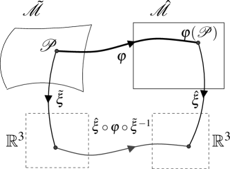
Figure 1: (Diffeo)-morphism. Points $\mathcal{P}$ in the device manifold ${\tilde{{\mathcal{M}}}}$ are mapped to points ${\varphi}(\mathcal{P})$ in the design manifold ${\hat{{\mathcal{M}}}}$ by the morphism (mapping) ${\varphi}$. The $\mathbb{R}^{3}$ coordinate representation of the morphism, is $\Lambda^{-1}=\hat{\xi}\circ{\varphi}\circ\tilde{\xi}^{-1}:\mathbb{R}^{3}\rightarrow\mathbb{R}^{3}$. This means that the design of the T-device is specified by ${\varphi}$, but that expression of that design in coordinate terms – the “blueprint” – is $\Lambda$.

III.1 Metrics and coordinate transformations

If we adhere to the traditional coordinate-based interpretation of T-Design, then we can transform the metric simply with the notional coordinate transform that we use to define our desired T-device. Coordinate transformations of representations of tensors depend on the differential relationships between the old and new coordinates, i.e.

$$x^{\alpha^{\prime}} =f(x^{\alpha})\qquad\textrm{then}\qquad\Lambda\indices{{}^{\alpha^{\prime}}_{\alpha}}=\frac{\partial f(x^{\alpha})}{\partial x^{\alpha}}.$$ (33)

So a metric ${g}$ and its inverse re-represented in new primed coordinates would be

$${g}\indices{{}_{\alpha^{\prime}\beta^{\prime}}} =\Lambda\indices{{}^{\alpha}_{\alpha^{\prime}}}{g}\indices{{}_{\alpha\beta}}\Lambda\indices{{}^{\beta}_{\beta^{\prime}}},$$ (34)

$${g}\indices{{}^{\alpha^{\prime}\beta^{\prime}}} =\Lambda\indices{{}^{\alpha^{\prime}}_{\alpha}}{g}\indices{{}^{\alpha\beta}}\Lambda\indices{{}^{\beta^{\prime}}_{\beta}}.$$ (35)

In the standard T-Design paradigm the coordinate transformation has the effect of changing our reference case geodesics into new, useful, device geodesics; then we need to adapt our material parameters from the reference values to those that give rise to the T-device metric ${g}_{\alpha^{\prime}\beta^{\prime}}$.

We have already seen that an expression of a metric ${g}_{\alpha\beta}$ can be inverted to give speed-squared matrix ${\mathfrak{C}}^{ij}$; thus the inverted T-device metric ${g}^{\alpha^{\prime}\beta^{\prime}}$ tells us what the T-device speed-squared matrix ${{\mathfrak{C}}^{\prime}}^{ij}$ must be. Our knowledge of whatever chosen physical system we want to build the device using then tells us what material properties are needed to achieve the necessary ${{\mathfrak{C}}^{\prime}}^{ij}$ and hence implement the T-device.

However, if any physical idea must be expressible in a way that is independent of coordinates; how can any claimed “coordinate transformation” hope to represent the design or specification of a new device? Although the coordinate transformation paradigm works from a purely practical standpoint, some coordinate transformations cannot be represented as a diffeomorphism – the transform from cartesian to polar coordinates is one such example. In what follows we present a more general and mathematically formal method which encapsulates the steps needed to rigorously implement the process of T-Design.

III.2 Metric induced by a diffeomorphism

The mathematical underpinning of all transformation theories is in fact not that of coordinate transformation, but that of a morphism $\varphi$ that maps a point $\mathcal{P}$ on a “device” manifold ${\tilde{{\mathcal{M}}}}$, to another point $\varphi(\mathcal{P})$ on a reference (“design”) manifold ${\hat{{\mathcal{M}}}}$, as seen in Fig. 1. A coordinate chart $\hat{\xi}:{\hat{{\mathcal{U}}}}\rightarrow\mathbb{R}^{3}$ maps a point $\mathcal{P}\in{\hat{{\mathcal{U}}}}\subset{\hat{{\mathcal{M}}}}$ to Euclidean space. Mappings exist from the manifolds ${\tilde{{\mathcal{M}}}}$ and ${\hat{{\mathcal{M}}}}$ into charts on $\mathbb{R}^{3}$, these are $\hat{\xi}:{\hat{{\mathcal{M}}}}\rightarrow\mathbb{R}^{3}$ at $\mathcal{P}$, and $\tilde{\xi}:{\tilde{{\mathcal{M}}}}\rightarrow\mathbb{R}^{3}$ at $\varphi(\mathcal{P})$. However, in T-Optics, $\varphi$ enables us to prescribe the electromagnetic medium in the device manifold ${\tilde{{\mathcal{M}}}}$ for (typically) a vacuum-like manifold ${\hat{{\mathcal{M}}}}$, before any discussion of coordinates Thompson et al. (2011a, b).

Our primary task here is to work out how to specify the device metric ${\tilde{g}}_{ij}$, as induced by $\varphi$, in terms of the reference/design metric ${\hat{g}}_{ij}$. Often ${\hat{g}}_{ij}$ will just be a flat Minkowski metric $\eta_{ij}$, but not always. The device metric $\tilde{g}$ is related to the design metric $\hat{g}$ by

$${\tilde{g}}_{\mathcal{P}}(X_{\mathcal{P}},Y_{\mathcal{P}}) =\left[\varphi^{\ast}{\hat{g}}\right](X_{\mathcal{P}},Y_{\mathcal{P}})={\hat{g}}(\varphi_{\ast}X_{\mathcal{P}},\varphi_{\ast}Y_{\mathcal{P}}),$$ (36)

where we have to (either) pullback the metric $\hat{g}$, or pushforward its arguments $X_{\mathcal{P}}$, $Y_{\mathcal{P}}$ using the diffeomorphism $\varphi$. With some thought, we can see that this should be the expected behaviour: what we usually are typically trying to achieve is to make interesting trajectories into the “new normal”. E.g. we make a cloak-like device structure in the laboratory, with specified cloak-like wave or ray paths, into an actual cloak by insisting its properties are such that those paths look to the outside world as if they were in an unremarkable piece of vacuum. I.e., we are trying to make a device (cloak) manifold ${\tilde{{\mathcal{M}}}}$ look like the design (vacuum) manifold ${\hat{{\mathcal{M}}}}$, and not the other way around. In contrast, the traditional transformation proceedure acts like an active transformation, and in our morphism picture is from the design space to the device space. As a consequence the traditional picture’s basic operation is specified by $\varphi^{-1}$ rather than $\varphi$, and in our notation would be written

$$\Lambda=\tilde{\xi}\circ\varphi^{-1}\circ\hat{\xi}^{-1} :\mathbb{R}^{3}\rightarrow\mathbb{R}^{3}.$$ (37)

This makes it clear that the traditional picture is an active transformation.

As we saw in the previous section, for our purposes the inverse of the metric, which is related to our speed squared matrix $\mathfrak{C}$, is more useful. In mathematical terminology, this is known as the co-metric, which we will denote ${\mathfrak{g}}$. The co-metric version of (36) uses the pushforward rather than the pullback, and is

$${\hat{\mathfrak{g}}}_{\varphi_{\ast}\mathcal{P}}(\varphi_{\ast}X_{\mathcal{P}},\varphi_{\ast}Y_{\mathcal{P}}) =\left[\varphi_{\ast}{\tilde{\mathfrak{g}}}\right](\varphi_{\ast}X_{\mathcal{P}},\varphi_{\ast}Y_{\mathcal{P}})={\tilde{\mathfrak{g}}}(X_{\mathcal{P}},Y_{\mathcal{P}}),$$ (38)

Although in a mathematical sense, this has defined everything we need, for practical calculations a matrix notation is more convenient. The first step in achieving this is to write down (36) and (38) in an indexed notation; after which a choice of coordinates leads us to the relevant matrix form. Notably, (36) can be written

$${\tilde{g}}\indices{{}_{\tilde{\mu}\tilde{\nu}}} =(\varphi^{\ast})\indices{{}^{\hat{\alpha}}_{\tilde{\mu}}}(\varphi^{\ast})\indices{{}^{\hat{\beta}}_{\tilde{\nu}}}~{}{\hat{g}}\indices{{}_{\hat{\alpha}\hat{\beta}}},$$ (39)

where

$$(\varphi^{\ast})\indices{{}^{\hat{\beta}}_{\tilde{\nu}}}=\left.\frac{\partial y^{\hat{\beta}}}{\partial x^{\tilde{\nu}}}\right|_{\mathcal{P}}.$$ (40)

Similarly, we can do the same for the co-metric ${\mathfrak{g}}$. Since it has raised (and not lowered) indices, this distinguishes the the co-metric from the metric, and so we can replace the ${\mathfrak{g}}$ with an ordinary ${g}$, which matches with the notation used for the inverse metric in previous sections. We then can write

$${\hat{{g}}}\indices{{}^{\hat{\alpha}\hat{\beta}}} =(\varphi_{\ast})\indices{{}^{\hat{\alpha}}_{\tilde{\mu}}}(\varphi_{\ast})\indices{{}^{\hat{\beta}}_{\tilde{\nu}}}~{}{\tilde{{g}}}\indices{{}^{\tilde{\mu}\tilde{\nu}}},$$ (41)

$${\tilde{{g}}}\indices{{}^{\tilde{\mu}\tilde{\nu}}} =((\varphi^{-1})_{\ast})\indices{{}^{\tilde{\mu}}_{\hat{\alpha}}}((\varphi^{-1})_{\ast})\indices{{}^{\tilde{\nu}}_{\hat{\beta}}}~{}{\hat{{g}}}\indices{{}^{\hat{\alpha}\hat{\beta}}},$$ (42)

where

$$((\varphi^{-1})_{\ast})\indices{{}^{\tilde{\nu}}_{\hat{\beta}}}=\left.\frac{\partial x^{\tilde{\nu}}}{\partial y^{\hat{\beta}}}\right|_{\varphi_{\ast}\mathcal{P}}.$$ (43)

Notably, if we were to replace the “$(\varphi)$” notation with a coordinate-transform mimicking “$\Lambda$”, then the operations done here, in this more sophisticated pushforward/ pullback would match the use in the so-called “coordinate transform” approach (see e.g. Kinsler and McCall (2014b)); albeit with the significant advantage of being better mathematically and physically motivated. Moreover, there is a further distinction to be emphasised. In two dimensions, for example, one can have charts $\phi_{1}:{\mathcal{M}}\rightarrow\mathbb{R}$ and $\phi_{2}:{\mathcal{M}}\rightarrow\mathbb{R}\otimes\mathbb{S}$ and the transition map $\phi_{2}\circ\phi_{1}^{-1}$ describing the transformation from Cartesian to polar coordinates. This coordinate transformation and the associated $\Lambda$ matrices can be readily inserted into (34) or (35) but this does not produce a T-device. Morphing points on a manifold, on the other hand, one can use a single coordinate chart $\hat{\xi}:{\mathcal{M}}\rightarrow\mathcal{U}$ and the transition function $\hat{\xi}\circ\varphi\circ\hat{\xi}^{-1}$ (cf. Fig. 1) to reach a well-defined, and useful, T-device, by morphing the metric according to (39). Also note that if the ‘morphism’ is to leave points on the manifold unchanged, then the $\varphi$ matrices are the identity, whereas the $\Lambda$ matrices associated with coordinate transformations need not be.

III.3 Transformations, Morphisms

It is critical to notice at this point that if we specify the morphism in terms of how one coordinate point is moved to another, then we are only adjusting distances; i.e. only adjusting the effective metric. This is because we have explicitly separated the general step of specifying the device by means of a morphism, from its chosen implementation in a particular physical system. As a result our design/morphism is only targetted at the speed-squared matrix ${\mathfrak{C}}\indices{{}^{ij}}$ (i.e. the inverse metric), and nothing else. It cannot directly specify how physical properties such as field values, material parameters, ratios, or impedances have been affected, since they are still undecided.

However, once we have taken the additional step of specifying the physical system (e.g. EM), we can use the morphism to tell us how physical properties will be changed, and how much freedom there might be. For example, choosing the usual kappa medium assumption of “${\epsilon}={\mu}$” in an electromagnetic scenario has implications for impedance Kinsler (2015a), but such an identification has nothing to do with the morphism itself, which says nothing about the $\epsilon:\mu$ ratio. Of course, given a specified physical system, it is possible to apply T-design techniques to transform fields and/or other properties independently Liu and Li (2015); Liu et al. (2013).

As described above, here we make an identification between the metric and the material properties, in the same way as introduced to T-Optics by Leonhardt and Philbin Leonhardt and Philbin (2006). This is essentially a “coordinate redefinition” step, which results from the choosing of a secondary map Thompson and T. (2016).

IV Examples

As noted above, typically T-devices are described with a “transformation” narrative, where we talk of transforming an unremarkable reference space into an interesting device space. Hence the typical description of a cloaking transformation being that of a point in a flat space being expanded and pushed outwards to form a disk, and where (outwardly) the inside of that disk (“core”) region is invisible.

In the more rigorous morphism language we instead represent the deformation that takes the device (or “laboratory”) space manifold (${\tilde{{\mathcal{M}}}}$), with its missing disk, and alters the metric on that manifold so as to “pull it inwards’. As a result ${\tilde{{\mathcal{M}}}}$ then acts as if it were like a design (i.e. apparent, or “reference”) manifold (${\hat{{\mathcal{M}}}}$) only missing a single point. This is the reverse narrative of the (usual) transformation one, and the mathematical and physical reasons for this were described in the previous section.

However, the reason why the usual transformation narrative is not without its uses is that non-trival reference manifolds might have metrics and geodesics with all kinds of interesting properties, involving ones that have foci, caustics, or that form loops. And whatever the exotic properties of our T-device might be in re-presenting the physical reality to an observer, it must be capable of being mapped onto that apparent manifold. By starting a design process with the intended (design) behaviour, and morphing (by pullback) to the device behaviour, we can guarantee that our aim is achievable, at least in principle. This specification means that the morphism should also have differentiable inverse, i.e. be a diffeomorphism.

In the examples below, the necessary device metric $\tilde{g}_{ij}$ can be calculated from the design metric $\hat{g}_{ij}$ using the components $(\varphi)\indices{{}^{i}_{l}}$ of the design morphism $\varphi$. Using square brackets to indicate a matrix-like representation, we find that

$$\begin{bmatrix}\tilde{g}_{ij}\end{bmatrix} =\begin{bmatrix}(\varphi^{\ast})\indices{{}^{l}_{i}}\end{bmatrix}\begin{bmatrix}\hat{g}_{lm}\end{bmatrix}\begin{bmatrix}(\varphi^{\ast})\indices{{}^{m}_{j}}\end{bmatrix}^{T},$$ (44)

$$\begin{bmatrix}\tilde{g}^{ij}\end{bmatrix} =\begin{bmatrix}((\varphi^{-1})_{\ast})\indices{{}^{i}_{l}}\end{bmatrix}\begin{bmatrix}\hat{g}^{lm}\end{bmatrix}\begin{bmatrix}((\varphi^{-1})_{\ast})\indices{{}^{j}_{m}}\end{bmatrix}^{T}=\begin{bmatrix}\tilde{\mathfrak{C}}^{ij}\end{bmatrix}.$$ (45)

Here the second line represents the next, more pragmatic step, where the inverse device metric is used to generate the speed-squared matrix $[\tilde{\mathfrak{C}}^{ij}]$ that we need to engineer using the relevant material properties. Note that this transformation also uses the $\varphi_{\ast}$ pushforward form of the inverseof the morphism, i.e. $\varphi^{-1}$. In the examples that follow, we will use the phrase “non-trivial” to describe any diffeomorphism components $((\varphi^{-1})_{\ast})\indices{{}^{i}_{l}}$ that differ from the identity transformation value of $\delta\indices{{}^{i}_{l}}$. For example, if we chose to restrict ourselves to a cylindrical geometry, with only radial transformations, the only non-trival components will be radial ones.

Further, we also show only ray examples, because strictly speaking only in the ray limit is the metric approach exact. In any case, the literature is already full of wave-cloak pictures for various degrees of approximation in the underlying model. A careful analysis demonstrating the effects of the neglected impedance terms and possibly non-trivial properties of the underlying space is no simple matter, and will be addressed elsewhere Kinsler (2015a, b).

IV.1 Cylindrical cloak

The cylindrical cloak first introduced by Pendry et al Pendry et al. (2006) is the most famous T-device. Its design is usually expressed as expanding a central point into a disk (or “core”) $r=R$ in diameter, while compressing its “halo” – the space between the point and the outer rim at $r=S$ accordingly. It therefore preserves the effective distance between inner and outer radii as being the same as (just) the outer radius. It is usually written in cylindrical coordinates, and a general form allowing for a variety of radial transformations is

$$\hat{r}={f}(\tilde{r}),\quad\hat{\theta}=\tilde{\theta},\quad\hat{z}=\tilde{z},$$ (46)

where $f(\tilde{r})$ is some suitably well behaved function increasing from $f(R)=0$ to $f(S)=S$; it is the derivative of this $f$ which specifies the only non-trivial morphism component $(\varphi^{\ast})\indices{{}^{r}_{r}}$.

In the original proposal Pendry et al. (2006), $f$ was simply the linear

$$f(\tilde{r})=\frac{S}{S-R}\left(\tilde{r}-R\right).$$ (47)

Here $\tilde{r},\tilde{\theta},\tilde{z}$ are the device coordinates where waves or rays are confined to $\tilde{r}>R$, and so hiding points where $\tilde{r}<R$. Otherwise, the coordinates $\hat{r},\hat{\theta},\hat{z}$ span the design space where waves or rays are allowed at any $\hat{r}>0$.

Let us assume for additional generality that we want the design spatial metric (i.e. the apparent metric of our device) to have independent radial, angular, and axial refractive index profiles $n(\hat{r})$, $m(\hat{\theta})$, $s(\hat{z})$. This allows us, for example, to consider adding a cloak to a 2D Maxwell’s fisheye device Sarbort and Tyc (2012); Luneburg (1964), where $m(\hat{\theta})=1$, $s(\hat{z})=1$ and $n(\hat{r})=n_{0}/[1+(r/r_{0})^{2}]$. Our design metric is then

$${d\hat{S}}^{2} =n^{2}(\hat{r}){d\hat{r}}^{2}+m^{2}(\hat{\theta})\hat{r}^{2}{d\hat{\theta}}^{2}+s^{2}(\hat{z}){d\hat{z}}^{2},$$ (48)

$$\textrm{or}\qquad\hat{g}\indices{{}_{ij}} =\begin{bmatrix}n^{2}&~{}~{}0~{}~{}&~{}~{}0~{}~{}\\ ~{}~{}0~{}~{}&m^{2}&~{}~{}0~{}~{}\\ 0&0&s^{2}\end{bmatrix}.$$ (49)

This means that whilst an outside observer with no reason to make complicating assumptions would presume geodesics which match those in the design spatial metric, that region can have properties that differ according to some morphism $\varphi$. A morphism $\varphi$ based on the transformation $f$ from (46) has the important (non trivial) component $(\varphi_{A})\indices{{}^{r}_{r}}=f^{\prime}=\partial f/\partial\tilde{r}$. With this, it hides the core region as a result of generating the required device spatial metric of

$${d\tilde{S}}^{2} =n^{2}(f(\tilde{r}))\left[\frac{df(\tilde{r})}{d\tilde{r}}\right]^{2}{d\tilde{r}}^{2}+m^{2}(\tilde{\theta})\left[\frac{f(\tilde{r})}{\tilde{r}}\right]^{2}\tilde{r}^{2}{d\tilde{\theta}}^{2}$$

$$\qquad\qquad\qquad\qquad\qquad\qquad+s^{2}(\tilde{z}){d\tilde{z}}^{2},$$ (50)

which, as should be expected, looks like (is) the same result as that obtained by the misleadingly named “coordinate transformation” approaches Cummer et al. (2009); Cai et al. (2007) based on equations like (46). This interval-style ${d{S}}^{2}$ metric can also be written in a matrix-like form, with $n\equiv n(f(\tilde{r}))$, $m\equiv m(\tilde{\theta})$, $s\equiv s(\tilde{z})$, i.e.

$$\tilde{g}\indices{{}_{ij}} =\begin{bmatrix}n^{2}{f^{\prime}}^{2}&0&~{}~{}0~{}~{}\\ 0&m^{2}f^{2}/\tilde{r}^{2}&~{}~{}0~{}~{}\\ 0&0&~{}~{}s^{2}~{}~{}\end{bmatrix}$$ (51)

As described above we can convert – by a simple inversion – this T-device metric into the corresponding speed-squared matrix, i.e.

$$\tilde{\mathfrak{C}}\indices{{}^{ij}} =\tilde{g}\indices{{}^{ij}}=\begin{bmatrix}\tilde{g}\indices{{}_{ij}}\end{bmatrix}^{-1}$$ (52)

Figure 2: Radial cloak based on the logarithmic function given in (53). One nice feature of this cloaking function is that it has both index and gradient matching at the outer boundary $S=eR$ of the halo.

We might, for example, use an alternate radial cloak using the logarithm function Ma et al. (2009) so that it could be more smoothly matched than the original (linear) radial cloak Pendry et al. (2006), at its outer boundary. The log radial cloak is designed using

$$F(\tilde{r}) =S\log\left[\tilde{r}/R\right],\quad\textrm{so that}\quad F^{\prime}(\tilde{r}) =S/\tilde{r}.$$ (53)

To work, this log radial cloak requires a fixed core-to-halo ratio so that $S=eR$. The mapping between $\tilde{r}$ and $\hat{r}$ is shown on fig. 2. The disadvantage of this design is that there is a stronger gradient at its interface with the core than with the original; for particular experimental implementations, this disadvantage may outweigh the benefits of its smoother matching at the outer boundary. This is because cloak performance can be strongly affected by imperfect implementation of the inner (core) boundary, although this would not be relevant in the near-miss case of a narrow beam that only passes through the outer part of the cloak halo.

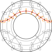
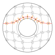
Figure 3: Comparison of the linear-radial Pendry et al. (2006) and log-radial cloaking transforms designed to match a flat space. Sample of ray trajectories and refractive index ellipses are shown. Figures provided by R.D. Topf.

So for an EM wave in this T-device cloak where we choose the case where the electric polarization is not aligned along $\theta$, we find that $\epsilon_{z},\epsilon_{r},\mu_{r},\mu_{\theta}$ are the controlling constitutive parameters. Therefore in cylindrical coordinates we have

$$\tilde{\mathfrak{C}}\indices{{}^{ij}}=\begin{bmatrix}\epsilon_{z}\mu_{\theta}&0&0\\ 0&\epsilon_{z}\mu_{r}&0\\ 0&0&\epsilon_{r}\mu_{\theta}\end{bmatrix}^{-1}=\begin{bmatrix}1/n^{2}{F^{\prime}}^{2}&0&~{}~{}0~{}~{}\\ 0&\tilde{r}^{2}/m^{2}F^{2}&~{}~{}0~{}~{}\\ 0&0&~{}~{}1/s^{2}~{}~{}\end{bmatrix}.$$ (54)

Alternatively, we might have chosen the complementary case where the magnetic field is not aligned along $\theta$.

For a scalar p-acoustics wave in the same cloaking T-device there is no scope for a choice of polarizations, unlike the EM case above. In cylindrical coordinates we have a unique specification for the constitutive parameters that is

$$\tilde{\mathfrak{C}}\indices{{}^{ij}}=\kappa_{o}\begin{bmatrix}\rho_{rr}&0&0\\ 0&\rho_{\theta\theta}&0\\ 0&0&\rho_{zz}\end{bmatrix}^{-1}=\begin{bmatrix}1/n^{2}{F^{\prime}}^{2}&0&~{}~{}0~{}~{}\\ 0&\tilde{r}^{2}/m^{2}F^{2}&~{}~{}0~{}~{}\\ 0&0&~{}~{}1/s^{2}~{}~{}\end{bmatrix}.$$ (55)

A comparison of the EM and scalar p-acoustics cases is instructive. In EM, for each of the two possible field polarizations we can implement the three necessary cloak parameters $\tilde{\mathfrak{C}}^{rr},\tilde{\mathfrak{C}}^{\theta\theta},\tilde{\mathfrak{C}}^{zz}$ using up to six constitutive parameters, i.e. we have three “spare” degrees of freedom. In contrast, the p-acoustic version has only four constitutive parameters with which to make up the three cloak parameters, i.e. only one degree of freedom: we could e.g. leave $\kappa_{o}$ untouched and engineer each of $\rho_{rr},\rho_{\theta\theta},\rho_{zz}$. This significantly impacts our ability to fine-tune the p-acoustic cloak in response to technological constraints.

A pentamode p-acoustics wave has additional constitutive freedom compared to the scalar version, since $\kappa$ is now matrix-like. In cylindrical coordinates, the same cloaking T-device has a specification for the constitutive parameters based on diagonal $\kappa^{ij}$ and ${\rho}\indices{{}^{k}_{l}}$ properties is

$$\tilde{\mathfrak{C}}\indices{{}^{ij}}=\begin{bmatrix}\frac{\kappa_{rr}}{\rho_{rr}}&0&0\\ 0&\frac{\kappa_{\theta\theta}}{\rho_{\theta\theta}}&0\\ 0&0&\frac{\kappa_{zz}}{\rho_{zz}}\end{bmatrix}=\begin{bmatrix}1/n^{2}{F^{\prime}}^{2}&0&~{}~{}0~{}~{}\\ 0&\tilde{r}^{2}/m^{2}F^{2}&~{}~{}0~{}~{}\\ 0&0&~{}~{}1/s^{2}~{}~{}\end{bmatrix}.$$ (56)

Note that $\kappa^{nj}$ and $\bar{\rho}\indices{{}_{n}^{i}}$ need not be diagonal as long as their product $\tilde{\mathfrak{C}}\indices{{}^{ij}}$ is.

However, despite caveats regarding impedance matching, the wave or ray “steering” performance of these implementations is as identical as the identical metrics upon which they are based; only their scattering properties are different.

In the case of heat diffusion, we can just implement the $\tilde{\mathfrak{C}}\indices{{}^{ij}}$ directly as the diffusion matrix

$$\tilde{\mathfrak{D}}\indices{{}^{ij}}=\frac{1}{\rho c_{p}}\left[{K}\indices{{}^{ij}}\right]=\begin{bmatrix}1/n^{2}{F^{\prime}}^{2}&0&~{}~{}0~{}~{}\\ 0&\tilde{r}^{2}/m^{2}F^{2}&~{}~{}0~{}~{}\\ 0&0&~{}~{}1/s^{2}~{}~{}\end{bmatrix},$$ (57)

with constant density $\rho$ and specific heat $c_{p}$, and an anistropic thermal conductivity $K\indices{{}^{ij}}$.

IV.2 Cloak on a sphere

Here our design space is a 2D spherical surface of radius $R$ which is most naturally expressed in spherical polar coordinates. Allowing for independent angular indices $T(\hat{\theta})$, $P(\hat{\phi})$, this has a design spatial metric which is

$$d\hat{S}^{2} =\left[T^{2}(\hat{\theta})\right]R^{2}d\hat{\theta}^{2}+\left[P^{2}(\hat{\phi})\right]R^{2}\sin^{2}(\hat{\theta})d\hat{\phi}^{2},$$ (58)

with the variation in polar angle $\hat{\theta}$ denoting lines of “longitude”, and variation in the azimuthal angle $\hat{\phi}$ being latitude. The sensible choice is to orient the coordinates so that both the missing point in the design (target) space, and the missing spherical cap in the device (laboratory) space, are centered on the pole. In this case we leave the azimuthal $\phi$ untouched so that $\tilde{\phi}=\hat{\phi}$, but offset and rescale the polar angle $\hat{\theta}$ so that

$$\hat{\theta}=f(\tilde{\theta})\quad\textrm{and}\qquad\tilde{\theta}=f^{-1}(\hat{\theta})=F(\hat{\theta}).$$ (59)

Thus the morphed device metric, with $(\varphi_{B})\indices{{}^{\theta}_{\theta}}=f^{\prime}(\tilde{\theta})=df(\tilde{\theta})/d{\tilde{\theta}}$, is

$$d{S}^{2} =\left[T(f(\tilde{\theta}))~{}{f^{\prime}(\tilde{\theta})}\right]^{2}~{}R^{2}d{\tilde{\theta}}^{2}$$

$$\qquad\qquad+\left[P(\tilde{\phi})\frac{\sin\left(f(\tilde{\theta})\right)}{\sin(\tilde{\theta})}\right]^{2}~{}R^{2}\sin^{2}(\tilde{\theta})d\phi^{2}.$$ (60)

This has been written so as to separate the part of the new T-device metric which encodes the necessary constitutive properties, (which have been put in square brackets) from that which encodes the spherical geometry. Our T-device needs the longitude component of rays (or waves) to see an index a factor of $f^{\prime}(\tilde{\theta})$ larger than the background; whereas the latitude component needs to see a different index depending on how close to the cloak core (at $\theta_{0}$) they are.

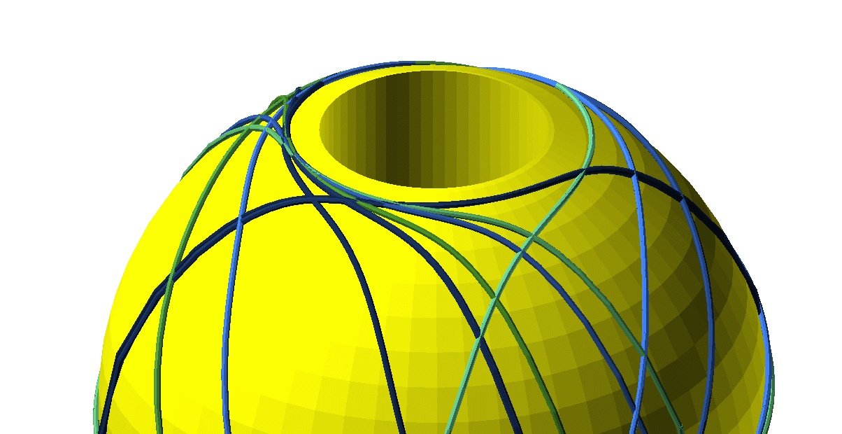
Figure 4: Radial cloak on a spherical surface, again based on a logarithmic function. A random selection ray paths are shown, all being forced by the cloak to avoid the core region which extends up to $20^{\circ}$ from the north pole, whilst also returning smoothly to their expected “great circle” paths outside the cloak halo at $e\times 20^{\circ}\simeq 54^{\circ}$.

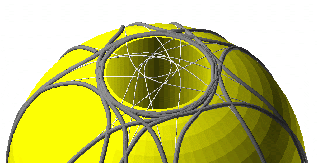
Figure 5: Radial cloak on a spherical surface, again based on a logarithmic function; however unlike fig. 4 the original spherical surface has a varying instead of a constant background index; this perturbs the ray paths. This figure shows only a long segment taken from a single ray path, which returns to the vicinity of the north pole to be cloaked (from) over and over again. The thin lines show the path the ray would have taken if the cloak were not present.

For example, with a standard linear transformation where $\tilde{\theta}=\alpha\hat{\theta}+\theta_{0}$, and with $T\equiv T(f(\tilde{\theta}))$ and $P\equiv P(\tilde{\phi})$, where $\alpha=1-\theta_{0}/\pi$, then the device metric must be

$$d\tilde{S}^{2} =\left[\frac{T}{\alpha}\right]^{2}~{}R^{2}d{\tilde{\theta}}^{2}+\left[P\frac{\sin\left(\frac{\tilde{\theta}-\theta_{0}}{\alpha}\right)}{\sin(\tilde{\theta})}\right]^{2}~{}R^{2}\sin^{2}(\tilde{\theta})d\tilde{\phi}^{2}.$$ (61)

An alternative cloaking deformation based on the logarithmic one used in subsection IV.1 could be $\tilde{\theta}=\theta_{0}\exp(\hat{\theta}/e\theta_{0})$. This morphism has taken a partial spherical manifold and morphed it into a (near) full sphere; thus the morphism applies only over $\tilde{\theta}\in(\theta_{0},e\theta_{0}]$ and (but) mimics the range $\hat{\theta}\in(0,e\theta_{0}]$. On the rest of the sphere, i.e. for angles $\theta\in(e\theta_{0},\pi]$, we have that $\tilde{\theta}=\hat{\theta}$. This gives a morphed (T-device) metric

$$d\tilde{S}^{2} =\left[\frac{Te\theta_{0}}{\tilde{\theta}}\right]^{2}R^{2}d{\tilde{\theta}}^{2}$$

$$\quad+\left[P\frac{\sin\left(e\theta_{0}\log\left\{\frac{\tilde{\theta}}{\theta_{0}}\right\}\right)}{\sin(\tilde{\theta})}\right]^{2}R^{2}\sin^{2}(\tilde{\theta})d\tilde{\phi}^{2},$$ (62)

where since the metric is diagonal, the ${\theta\theta}$ and ${\phi\phi}$ components of the inverse-metric $\tilde{g}^{ij}$, speed squared $\tilde{\mathfrak{C}}^{ij}$, or diffusion ${\mathfrak{D}}^{ij}$ matrices, are just given by the inverse of square bracket terms. These inverses are in essence just rescaling factors for the speeds $c_{\theta}$ and $c_{\phi}$ on the sphere in the angular and azimuthal directions. Thus the logarithmically cloaked sphere, in the transformed region, needs to have its material parameters modified so that

$$\frac{\tilde{c}_{\theta}}{\hat{c}_{\theta}}=\sqrt{\frac{\tilde{\mathfrak{C}}^{\theta\theta}}{\hat{\mathfrak{C}}^{\theta\theta}}} =\left[\frac{\tilde{\theta}}{e\theta_{0}}\right],$$ (63)

$$\frac{\tilde{c}_{\phi}}{\hat{c}_{\phi}}=\sqrt{\frac{\tilde{\mathfrak{C}}^{\phi\phi}}{\hat{\mathfrak{C}}^{\phi\phi}}} =\left[\frac{\sin(\tilde{\theta})}{\sin\left(e\theta_{0}\log\left\{\frac{\tilde{\theta}}{\theta_{0}}\right\}\right)}\right].$$ (64)

As before, we can choose implement this anisotropic speed profile for either EM or acoustics following a similar procedure as for the ordinary cylindrical cloak; we might equally as easily follow the rules to work out the material parameters needed for a heat diffusion cloak.

A depiction of this cloak, implemented on a featureless sphere where $T=P=1$, is shown in fig. 4, and showing a variety of deformed – cloaked – great circle geodesic trajectories. For more complicated spheres, such as ones with a pre-existing index profiles that vary over the surface, the geodesics will no longer be great circles. Cloaking on such a sphere is displayed on fig. 5. In this example a single ray trajectory will now travel widely over the surface in a complicated manner, and so returns again and again to the north pole region to be cloaked and recloaked in different ways and from different directions.

IV.3 Topographic transformation

Imagine we wish to control our waves or rays so that they appear to be travelling along a designer bumpy three dimensional landscape, even though they remain confined to a planar device space, albeit a plane with appropriately modulated properties. If the height of the virtual landscape is defined by the function $\hat{z}=h(\hat{x},\hat{y})$, then the required 2D metric that mimics it is based on $(\varphi^{\ast}_{C})\indices{{}^{z}_{x}}=\partial h/\partial\tilde{x}$ and $(\varphi^{\ast}_{C})\indices{{}^{z}_{y}}=\partial h/\partial\tilde{y}$, being

$$d\hat{S}^{2} =\left[1+\left(\frac{\partial h}{\partial{\tilde{x}}}\right)^{2}\right]d{\tilde{x}}^{2}+\left[1+\left(\frac{\partial h}{\partial{\tilde{y}}}\right)^{2}\right]d{\tilde{y}}^{2}$$

$$\qquad\qquad\qquad+2\left[\left(\frac{\partial h}{\partial{\tilde{x}}}\right)\left(\frac{\partial h}{\partial{\tilde{y}}}\right)\right]d\tilde{x}~{}d\tilde{y}.$$ (65)

If, for example we wished to mimic a parabolic or hyperbolic landscape, defined by the height function $h_{1}(\tilde{x},\tilde{y})=\alpha\tilde{x}^{2}+\beta\tilde{y}^{2}$, then the required device metric is

$$d\hat{S}^{2} =\left[1+4\alpha^{2}\tilde{x}^{2}\right]d{\tilde{x}}^{2}+\left[1+4\beta^{2}\tilde{y}^{2}\right]d{\tilde{y}}^{2}$$

$$\qquad\qquad\qquad+2\left[4\alpha\beta\tilde{x}\tilde{y}\right]~{}d\tilde{x}~{}d\tilde{y}.$$ (66)

The metric components ${g}_{xx}$, ${g}_{xy}$, and ${g}_{yy}$ can then be read off directly from this result. The components of ${\mathfrak{C}}^{ij}$ or ${\mathfrak{D}}^{ij}$ can then be determined, being given by the inverse of the matrix

$$\begin{bmatrix}{g}_{xx}&{g}_{xy}\\ {g}_{xy}&{g}_{yy}\end{bmatrix}=\begin{bmatrix}1+4\alpha^{2}\tilde{x}^{2}&4\alpha\beta\tilde{x}\tilde{y}\\ 4\alpha\beta\tilde{x}\tilde{y}&1+4\beta^{2}\tilde{y}^{2}\end{bmatrix}.$$ (67)

Alternatively, if we wished to mimic a landscape with a deep well (or peak) as defined by the height function $h_{2}(\tilde{x},\tilde{y})=\gamma/(1+\alpha\tilde{x}^{2}+\beta\tilde{y}^{2})$, then the required device metric is

$$d\hat{S}^{2} =\left[1+\left(\frac{4\alpha^{2}}{\gamma^{2}}\right)\tilde{x}^{2}~{}h_{2}(\tilde{x},\tilde{y})^{4}\right]d{\tilde{x}}^{2}$$

$$\quad\qquad+\left[1+\left(\frac{4\beta^{2}}{\gamma^{2}}\right)\tilde{y}^{2}~{}h_{2}(\tilde{x},\tilde{y})^{4}\right]d{\tilde{y}}^{2}$$

$$\qquad\qquad\qquad+2\left[\left(\frac{4\alpha\beta}{\gamma^{2}}\right)\tilde{x}\tilde{y}~{}h_{2}(\tilde{x},\tilde{y})^{4}\right]~{}d\tilde{x}~{}d\tilde{y}.$$ (68)

Of course, many other landscapes can be imagined, for example those considered when making surface wave cloaks Mitchell-Thomas et al. (2013, 2014); Horsley et al. (2014) or geodesic lenses Sarbort and Tyc (2012); Kinsler et al. (2012); Luneburg (1964).

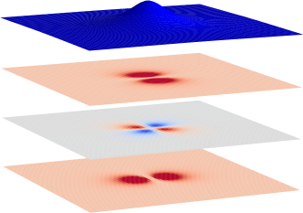
Figure 6: A 3D depiction of a topographic design manifold (top), given by (68) with $\alpha=\beta=20$ and $\gamma=1$. The necessary metric properties of the planar device (manifold), i.e. the $\tilde{x}\tilde{x}$, $\tilde{x}\tilde{y}$, and $\tilde{y}\tilde{y}$ components, are given as color-coded surfaces below. These metric components, in a flat (planar) device, mimic the distorted design manifold.

This kind of landscape T-Design might lead us to consider the reverse case: can we, by transformation, modulate the properties of a bumpy but locally isotropic (device) sheet embedded in 3D – a pre-existing landscape of the type discussed above, with height $z=h(x,y)$ – so that it is designed to appear as if it were instead a flat sheet in 2D? The answer is, in general, an emphatic no; although this can be done in some specific cases: i.e. the geodesic lenses mentioned above.

Imagine we have waves or rays travelling along some kind of bumpy landscape that we wish to re-map to a flat space. Crucially, in some places, for example, the local curvature will cause some geodesics to converge at and through a focus. Now no matter what diffeomorphism we apply, we cannot remove that focus, but only shift its position. Further, since any collection of geodesics in a flat space can at most all share only a single focus, as soon as a landscape is such that if anywhere a collection of geodesics share two foci, we cannot (in general) diffeomorphically transform from one to the other.

IV.4 Focus transformation

We can imagine representing device that focuses in the 2D plane as a T-Design by embedding it in 3D and twisting the space along the focal axis, as depicted in fig. 7. With $z$ chosen as the focal axis, points are twisted off the $x$-axis into the $xy$-plane, using a rotation defined by

$$\hat{z} =\tilde{z},~{}~{}\quad\hat{x}=\tilde{x}\cos(\Phi\tilde{z}+\phi),~{}~{}\quad\hat{y}=\tilde{x}\sin(\Phi\tilde{z}+\phi).$$ (69)

The device space of $\tilde{z},\tilde{x}$ will then mimic the behaviour design space’s twisted version embedded in $\hat{z},\hat{x},\hat{y}$. This will involve periodic refocusings at $\Phi\tilde{z}+\phi=(2n+1)\pi/2$. This T-Design specification means that the two spaces differ in a nontrivial way (only) due to $(\varphi^{\ast}_{E})\indices{{}^{x}_{x}}$, $(\varphi^{\ast}_{E})\indices{{}^{x}_{z}}$, $(\varphi^{\ast}_{E})\indices{{}^{y}_{x}}$, and $(\varphi^{\ast}_{E})\indices{{}^{y}_{z}}$. These give

$${d\hat{z}} ={d\tilde{z}},$$ (70)

$${d\hat{x}} =-\Phi\tilde{x}\sin(\Phi\tilde{z}+\phi){d\tilde{z}}+\cos(\Phi\tilde{z}+\phi){d\tilde{x}},$$ (71)

$${d\hat{y}} =~{}~{}~{}\Phi\tilde{x}\cos(\Phi\tilde{z}+\phi){d\tilde{z}}+\sin(\Phi\tilde{z}+\phi){d\tilde{x}},$$ (72)

and so

$${d\hat{S}}^{2} ={d\hat{x}}^{2}+{d\hat{y}}^{2}+{d\hat{z}}^{2}$$ (73)

$$=\left(1+\Phi^{2}\tilde{x}^{2}\right){d\tilde{z}}^{2}+{d\tilde{x}}^{2},$$ (74)

so we have (almost) reinvented the parabolic index waveguide; the difference being that only the $z$-directed index profile is modulated. The resulting anisotropy means that – as is obvious from the transformation used – the structure preserves path lengths and will have no spatial dispersion in the ray limit.

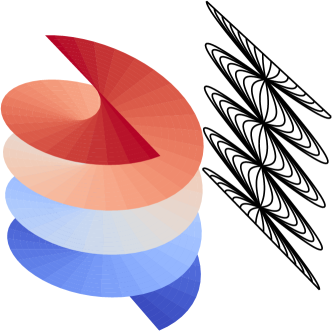
Figure 7: A 3D depiction of the helical design manifold used in the focus transformation, with a $\hat{z}$-dependent colour gradient to aid interpretation, and the resulting ray trajectories in $\tilde{x}\tilde{z}$-plane of the device (manifold).

The $x,z$ speed squared matrix for the anisotropic material required for this device design when applied to waves or rays is then

$${\mathfrak{C}}\indices{{}^{ij}}=c^{2}\begin{bmatrix}1&0\\ 0&1+\Phi^{2}\tilde{x}^{2}\end{bmatrix}^{-1}.$$ (75)

Further, we could note that this transformation acts rather like a 2D projection of the helical transformation discussed by McCall et al. McCall et al. (2016).

Note that at a given focus point $\tilde{z}_{i}$, the transformation projects multiple points (actually the entire $\hat{y}$-axis) down to a single point in the device, namely $\tilde{z}=\tilde{z}_{i}$ and $\tilde{x}=0$. Indeed, the device manifold consists of the $\tilde{x}\tilde{z}$-plane, but with the set of all points consisting of the lines along $\tilde{z}=[(2n+1)\pi/2-\phi]/\Phi$ except when $\tilde{x}=0$ removed. Nevertheless, rays passing through these foci are still distinguishable from each other by their direction. Remarkably, we can also see that the device properties are insensitive to the chosen phase offset $\phi$.

V Conclusion

Here we have shown the extent to which all the distinct types of transformation design might be repackaged into a general formalism. Although this process has necessarily involved approximations, we have shown that it is possible to make a clear distinction between the mathematical design step and the subsequent choice of which physical model is used to implement it.

Indeed, from the perspective given here, there is absolutely nothing “magic” about transformation optics, acoustics, or any of the other transformation domains – as long as we are prepared to tolerate approximations. If we have a pre-specified metric, then we can map this directly to a speed-squared matrix and use our knowledge of materials (or of metamaterials) to work out an implementation. Alternatively, and this is the usual case, if we have a useful scheme for reconfiguring the flow or location of the light or acoustic waves (or rays), then we can simply transform our design (“reference”) metric – usually the vacuum, but this is not a requirement – directly into the necessary device metric. This process involves the calculation of only a couple of matrix multiplications at each point in the transformed domain. Then, as before, the demands of any specific implementation are straightforward to identify.

Notably, we can see that if we eschew issues of impedance handling and changes in volume measure the wave and ray transformation procedures to be used are the same. This is not to deny the importance of impedance, merely to note the similarities between transformations of waves and rays. Further, the “obvious” process of matched modulation of both constitutive parameters – e.g. $\epsilon$ and $\mu$ in optics, $\kappa$ and $\rho$ in acoustics – gives the natural choice of impedance mismatch, even if the design intent is only for a ray T-device.

As it stands here, we only consider purely spatial transformations. However, it has already been shown McCall et al. (2011); Kinsler and McCall (2014a, b) that an extension to spacetime transformations can be done in a relatively straightforward way, at least in the 1+1D case. In contrast, spacetime transforms of dispersive Gratus et al. (2016) and diffusive systems are more problematic, and is an area we are actively investigating.

Appendix: Transforming Metrics

Take a vector space $V$ with a basis $\{{\bf e}_{\alpha}\}$. A basis of the dual space $V^{*}$ is a set of co-vectors $\{{\bm{\omega}}^{\beta}\}$ satisfying ${\bm{\omega}}^{\beta}({\bf e}_{\alpha})=\delta^{\beta}_{~{}\alpha}$.

Take an $n$-dimensional manifold $\cal M$ with a coordinate chart $\phi:{\cal U}\to{\mathbb{R}}^{n}$, i.e. $\phi(p)=\{x^{\alpha}(p)\}$.

A coordinate basis $\{\partial_{\alpha}\}$ at $p\in{\cal M}$ is associated with a set of coordinate functions $x^{\alpha}:{\cal U}\to{\mathbb{R}}$.

Take a function $f:{\cal M}\to{\mathbb{R}}$. Tangent vectors in $T_{p}{\cal M}$, the tangent (vector) space at $p$, act on such functions, to produce the number $v(f)$. With respect to the coordinate basis, $v(f)=v^{\alpha}\partial_{\alpha}f$.

If $T^{*}_{p}{\cal M}$ is the co-tangent space at $p$, then the 1-form $df\in T^{*}_{p}{\cal M}$ is defined via $df(v)=v(f)$. If we define $\{dx^{\beta}\}$ to be the basis dual to $\{\partial_{\alpha}\}$ (i.e. $dx^{\beta}(\partial_{\alpha})=\delta^{\beta}_{~{}\alpha}$), then $df=\partial_{\alpha}fdx^{\alpha}$.

A diffeomorphism $\varphi:{\cal M}\to{\cal N}$ induces the pull-back of functions from $\cal N$ to $\cal M$ according to $\varphi^{*}f(p)=f\circ\varphi(p)$.

The diffeomorphism also induces the push-forward of vectors $v\in T_{p}{\cal M}$ according to $\varphi_{*}v(f)=v(\varphi^{*}f)$. In components $(\varphi_{*}v)^{\mu}\partial_{\mu}=v^{\alpha}(\varphi_{*})^{\mu}_{~{}\alpha}\partial_{\mu}$, where $(\varphi_{*})^{\mu}_{~{}\alpha}=\partial y^{\mu}/\partial x^{\alpha}$, and $y^{\mu}$ is a coordinate function on $\cal N$ associated with $\varphi(p)$. It also induces the pull-back of 1-forms $df\in T^{*}_{\varphi(p)}{\cal N}$ according to $(\varphi^{*}df)(v)=df(\varphi_{*}v)$. In components $(\varphi^{*}df)_{\alpha}dx^{\alpha}=(df)_{\mu}(\varphi^{*})^{\mu}_{~{}\alpha}dx^{\alpha}$, where $(\varphi^{*})^{\mu}_{~{}\alpha}=\partial y^{\mu}/\partial x^{\alpha}$. Note that $(\varphi_{*})^{\mu}_{~{}\alpha}=(\varphi^{*})^{\mu}_{~{}\alpha}$. The positioning of the $*$ indicates whether we are pushing forward a vector or pulling back a 1-form.

A metric on ${\cal N}$ is a symmetric bilinear function of vectors, i.e. $g:T_{p}{\cal N}\times T_{p}{\cal N}\rightarrow{\mathbb{R}}$. If $\{dy^{\mu}\}$ is a coordinate co-basis of forms spanning $T^{*}_{\varphi(p)}{\cal N}$, then $g=g_{\mu\nu}dy^{\mu}\otimes dy^{\nu}$, where $g_{\mu\nu}=g_{\nu\mu}$. This metric can be pulled-back to $\cal M$ via $\varphi^{*}g(u,v)=g(\varphi_{*}u,\varphi_{*}v)$, where $u,v\in T_{p}{\cal M}$. Denoting this induced metric as ${\tilde{g}}=\varphi^{*}g$ we have, with respect to coordinate bases at $p\in\cal M$ and $\varphi(p)\in\cal N$, ${\tilde{g}}_{\alpha\beta}=(\varphi^{*})^{\mu}_{~{}\alpha}(\varphi^{*})^{\nu}_{~{}\beta}g_{\mu\nu}$.

A co-metric on $\cal M$ is a symmetric bilinear function of co-vectors, i.e. ${g}:T^{*}_{p}{\cal M}\times T^{*}_{p}{\cal M}\rightarrow{\mathbb{R}}$.

If $\{\partial_{\alpha}\}$ is a coordinate basis of vectors spanning $T_{p}{\cal M}$, then ${g}=g^{\alpha\beta}\partial_{\alpha}\otimes\partial_{\beta}$, where $g^{\alpha\beta}=g^{\beta\alpha}$. This co-metric can be pushed-forward to $\cal N$ via $\varphi_{*}{g}(\lambda,\rho)={g}(\varphi^{*}\lambda,\varphi^{*}\rho)$, where $\lambda,\rho\in T^{*}_{\varphi(p)}{\cal N}$. Denoting this induced co-metric as ${\tilde{g}}=\varphi_{*}{g}$ we have, with respect to coordinate bases in $\cal M$ and $\cal N$, ${\tilde{g}}^{\mu\nu}=(\varphi_{*})^{\mu}_{~{}\alpha}(\varphi_{*})^{\nu}_{~{}\beta}g^{\alpha\beta}$.

Now let’s work in a single manifold $\cal M$ equipped with a metric $g$. A vector $u\in T_{p}{\cal M}$ can be assigned a ‘squared length’ $u^{2}=g(u,u)$. In $T^{*}_{p}{\cal M}$ choose a co-vector ${u}$ such that ${u}(u)=g(u,u)$. A natural choice of co-metric is then one which sets ${g}({u},{u})=g(u,u)={u}(u)$. In that case it is easily shown that $u={g}(~{},{u})$, ${u}=g(u,~{})$ and ${g}^{\alpha\gamma}g_{\gamma\beta}=\delta^{\alpha}_{~{}\beta}$, where $\{e_{\beta}\}$ and $\{\omega^{\alpha}\}$ are respectively a basis of $T_{p}{\cal M}$ and a co-basis of $T^{*}_{p}{\cal M}$, i.e. $\omega^{\alpha}(e_{\beta})=\delta^{\alpha}_{~{}\beta}$. It then makes sense to refer to ${g}$ as the inverse of $g$.

Summary: you can pull-back a metric from $\cal N$ to $\cal M$, and you can push-forward a co-metric from $\cal M$ to $\cal N$. In a space equipped with a metric $g$ there is a natural co-metric ${g}$ which is the inverse of $g$ (i.e. $g$ takes $u$ to ${u}$, and ${g}$ takes ${u}$ back to $u$).

References

-
Pendry et al. (2006)
J. B. Pendry,
D. Schurig, and
D. R. Smith,
Science 312, 1780 (2006),
doi:10.1126/science.1125907. -
Leonhardt (2006)
U. Leonhardt,
Science 312, 1777 (2006),
doi:10.1126/science.1126493. -
McCall et al. (2011)
M. W. McCall,
A. Favaro,
P. Kinsler, and
A. Boardman,
J. Opt. 13, 024003 (2011),
doi:10.1088/2040-8978/13/2/024003. -
Kinsler and
McCall (2014a)
P. Kinsler and
M. W. McCall,
Ann. Phys. (Berlin) 526, 51 (2014a),
arXiv:1308.3358,
doi:10.1002/andp.201300164. -
Gratus et al. (2016)
J. Gratus,
P. Kinsler,
M. McCall, and
R. T. Thompson,
New J. Phys. 18, 123010 (2016),
arXiv:1608.00496,
doi:10.1088/1367-2630/18/12/123010. -
Fridman et al. (2012)
M. Fridman,
A. Farsi,
Y. Okawachi, and
A. L. Gaeta,
Nature 481, 62 (2012),
arXiv:1107.2062,
doi:10.1038/nature10695. -
Lukens et al. (2014)
J. M. Lukens,
A. J. Metcalf,
D. E. Leaird,
and A. M.
Weiner,
Optica 1, 372 (2014),
doi:10.1364/OPTICA.1.000372. -
Chremmos (2014)
I. Chremmos,
Opt. Lett. 39, 4611 (2014),
doi:10.1364/OL.39.004611. -
Jabar et al. (2015)
M. S. A. Jabar,
B. A. Bacha, and
I. Ahmad,
Laser Phys. 25, 065405 (2015),
doi:10.1088/1054-660X/25/6/065405. -
Zhang et al. (2011)
S. Zhang,
C. Xia, and
N. Fang,
Phys. Rev. Lett. 106, 024301 (2011),
doi:10.1103/PhysRevLett.106.024301. -
Sanchis et al. (2013)
L. Sanchis,
V. M. García-Chocano,
R. Llopis-Pontiveros,
A. Climente,
J. Martínez-Pastor,
F. Cervera, and
J. Sánchez-Dehesa,
Phys. Rev. Lett. 110, 124301 (2013),
doi:10.1103/PhysRevLett.110.124301. -
Guenneau et al. (2012)
S. Guenneau,
C. Amra, and
D. Veynante,
Opt. Express 20, 8207 (2012),
doi:10.1364/OE.20.008207. -
Schittny et al. (2015)
R. Schittny,
A. Niemeyer,
M. Kadic,
T. Bückmann,
A. Naber, and
M. Wegener,
Optica 2, 84 (2015),
doi:10.1364/OPTICA.2.000084. -
Kinsler and
McCall (2014b)
P. Kinsler and
M. W. McCall,
Phys. Rev. A 89, 063818 (2014b),
arXiv:1311.2287,
doi:10.1103/PhysRevA.89.063818. -
Kinsler (2009)
P. Kinsler,
Phys. Rev. A 79, 023839 (2009),
arXiv:0901.2466,
doi:10.1103/PhysRevA.79.023839. -
Kinsler and McCall (2015)
P. Kinsler and
M. W. McCall,
Photon. Nanostruct. Fundam. Appl. 15, 10 (2015),
doi:10.1016/j.photonics.2015.04.005. -
Sarbort and Tyc (2012)
M. Sarbort and
T. Tyc,
J. Opt. 14, 075705 (2012),
doi:10.1088/2040-8978/14/7/075705. -
Kinsler (2013)
P. Kinsler
(2013),
“Deriving the time-dependent Schrödinger m- and p-equations from the Klein-Gordon equation”,
arXiv:1309.3427. - Kittel (2004) C. Kittel, Introduction to Solid State Physics (Wiley, 2004), 8th ed., ISBN 978-0-471-41526-8.
-
Norris (2012)
A. N. Norris,
Appl. Phys. Lett. 100, 066101 (2012),
wrt [Appl. Phys. Lett. 97, 044101 (2010)],
doi:10.1063/1.3681945. -
Norris (2008)
A. N. Norris,
Proc. Royal Soc. A 464, 2411 (2008),
doi:10.1098/rspa.2008.0076. -
Flanders (1963)
H. Flanders,
Differential Forms with Applications to the Physical
Sciences (Academic Press, New York,
1963),
(reprinted by Dover, 2003). -
Zentgraf et al. (2010)
T. Zentgraf,
J. Valentine,
N. Tapia,
J. Li, and
X. Zhang,
Adv. Mat. 22, 2561 (2010),
doi:10.1002/adma.200904139. -
McCall et al. (2016)
M. W. McCall,
P. Kinsler, and
R. D. M. Topf,
J. Opt. 18, 044017 (2016),
doi:10.1088/2040-8978/18/4/044017. -
Kinsler et al. (2012)
P. Kinsler,
J. Tan,
T. C. Y. Thio,
C. Trant, and
N. Kandapper,
Eur. J. Phys. 33, 1737 (2012),
arXiv:1206.0003,
doi:10.1088/0143-0807/33/6/1737. -
Thompson
et al. (2011a)
R. T. Thompson,
S. A. Cummer,
and
J. Frauendiener,
J. Opt. 13, 024008 (2011a),
doi:10.1088/2040-8978/13/2/024008. -
Thompson
et al. (2011b)
R. T. Thompson,
S. A. Cummer,
and
J. Frauendiener,
J. Opt. 13, 055105 (2011b),
doi:10.1088/2040-8978/13/5/055105. -
Kinsler (2015a)
P. Kinsler
(2017a),
“Cloak Imperfect: Impedance”,
arXiv:1708.01071. -
Liu and Li (2015)
F. Liu and
J. Li,
Phys. Rev. Lett. 114, 103902 (2015),
doi:10.1103/PhysRevLett.114.103902. -
Liu et al. (2013)
F. Liu,
Z. Liang, and
J. Li,
Phys. Rev. Lett. 111, 033901 (2013),
doi:10.1103/PhysRevLett.111.033901. -
Leonhardt and Philbin (2006)
U. Leonhardt and
T. G. Philbin,
New J. Phys. 8, 247 (2006),
arXiv:cond-mat/0607418,
http://iopscience.iop.org/1367-2630/8/10/247/. -
Thompson and T. (2016)
M. F. Thompson and
R. T.,
Phys. Rev. D 93, 124026 (2016),
doi:10.1103/PhysRevD.93.124026. -
Kinsler (2015b)
P. Kinsler
(2015b),
in progress: GLOAK, “Cloak Imperfect: Determinant”. - Luneburg (1964) R. K. Luneburg, Mathematical Theory of Optics (University of California Press, Berkeley, CA, 1964).
-
Cummer et al. (2009)
S. A. Cummer,
R. Liu, and
T. J. Cui,
J. Appl. Phys. 105, 056102 (2009),
doi:10.1063/1.3080155. -
Cai et al. (2007)
W. Cai,
U. K. Chettiar,
A. V. Kildishev,
V. M. Shalaev,
and G. W.
Milton,
Appl. Phys. Lett. 91, 111105 (2007),
doi:10.1063/1.2783266. -
Ma et al. (2009)
J. J. Ma,
X. Y. Cao,
K. M. Yu, and
T. Liu,
Prog. Electromagn. Res. PIER M 9, 177 (2009),
doi:10.2528/PIERM09091405. -
Mitchell-Thomas
et al. (2013)
R. C. Mitchell-Thomas,
T. M. McManus,
O. Quevedo-Teruel,
S. A. R. Horsley,
and Y. Hao,
Phys. Rev. Lett. 111, 213901 (2013),
doi:10.1103/PhysRevLett.111.213901. -
Mitchell-Thomas
et al. (2014)
R. C. Mitchell-Thomas,
O. Quevedo-Teruel,
T. M. McManus,
S. A. R. Horsley,
and Y. Hao,
Opt. Lett. 39, 3551 (2014),
doi:10.1364/OL.39.003551. -
Horsley et al. (2014)
S. A. R. Horsley,
I. R. Hooper,
R. C. Mitchell-Thomas,
and
O. Quevedo-Teruel,
Sci. Rep. 4, 4876 (2014),
doi:10.1038/srep04876.