An iterative method to reconstruct the refractive index of a medium from time-of-flight measurements

Abstract

The article deals with a classical inverse problem: the computation of the refractive index of a medium from ultrasound time-of-flight (TOF) measurements. This problem is very popular in seismics but also for tomographic problems in inhomogeneous media. For example ultrasound vector field tomography needs a priori knowledge of the sound speed. According to Fermat’s principle ultrasound signals travel along geodesic curves of a Riemannian metric which is associated with the refractive index. The inverse problem thus consists of determining the index of refraction from integrals along geodesics curves associated with the integrand leading to a nonlinear problem. In this article we describe a numerical solver for this problem scheme based on an iterative minimization method for an appropriate Tikhonov functional. The outcome of the method is a stable approximation of the sought index of refraction as well as a corresponding set of geodesic curves. We prove some analytical convergence results for this method and demonstrate its performance by means of several numerical experiments. Another novelty in this article is the explicit representation of the backprojection operator for the ray transform in Riemannian geometry and its numerical realization relying on a corresponding phase function that is determined by the metric. This gives a natural extension of the conventional backprojection from 2D computerized tomography to inhomogeneous geometries.

1 Introduction

In this article we consider the inverse problem of computing the refractive index of a medium from ultrasound time-of-flight (TOF) measurements. On the one side this task is a tomographic problem of its own and often called the inverse kinematic problem which has important applications, e.g. in seismics. On the other side the knowledge of the sound speed, resp. refractive index, of an object $M\subset\mathbb{R}^{2}$ under consideration is essential for inverse problems in inhomogeneous media such as photoacoustic or ultrasound vector tomography. The idea is very simple: an ultrasound signal is emitted at a transmitter $A$ and its travel time is acquired at a detector $B$, see Figure 1. Of course the TOF depends of the sound speed $c(x)$ in the medium. The refractive index $n(x)=c_{0}/c(x)$, where $c_{0}$ denotes the constant sound speed of a reference medium like water or air outside the object, causes refractions of the ultrasound beam. Assuming a constant $n$ (e.g. by setting $n=1$) in applications such as photoacoustic or vector tomography hence might cause severe artifacts. We emphasized this in Figure 1. There, the blue triangle would be detected at the wrong place if we assume that the ultrasound signal travels along a straight line and that there is no refraction at all.

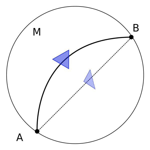
Fig. 1: TOF tomography measures the travel time a ultrasound signal needs to propagate from a source point $A$ to a detector $B$. If $n\not=1$, then the signal no longer travels along straight lines and reconstructions which neglect refraction show artifacts. E.g. the blue triangle would be detected at the wrong (dotted) place if we assumed straight lines as signal paths.

Let us briefly illuminate the situation in vector tomography. Norton [23] derived as mathematical model to compute a solenoidal vector field $v$ from TOF measurements the Doppler transform along straight lines

$$Dv(\ell)=\int_{\ell}\frac{\mathrm{d}l(x)}{c(x)+\langle v(x),\theta\rangle},$$

where $\theta$ denotes the vector of direction of the line $\ell$ which connects the points $A$ and $B$. Hence, to solve the inverse problem of computing $v$ from data $Dv$ it is necessary to know the sound speed $c(x)$. But Fermat’s pronciple says that the propagation paths are geodesic curves of the Riemannian metric

(1) $$\mathrm{d}s^{2}=n^{2}(x)\,|\mathrm{d}x|^{2}$$

leading to an improved model

$$Dv(\gamma)=\int_{\gamma}\frac{\mathrm{d}l(x)}{c(x)+\langle v(x),\dot{\gamma}(x)\rangle},$$

where $\gamma$ is a geodesic curve associated with the metric (1) and connecting the points $A$ and $B$. The problem now arises that the integrand determines the integration curve $\gamma$ turning the inverse problem into a nonlinear one. Also in photoacoustic tomography a variable sound speed leads to quite other analysis and numerics, see e.g. [1, 27]. Hence, following Fermat’s principle, then instead of the Euclidean space $(M,g_{0})$ with the Euclidean metric tensor $g_{0}=(\delta_{ij})$, we have to consider the Riemannian manifold $(M,g)$ with metric tensor $g_{ij}(x)=n^{2}(x)\delta_{ij}$.
This is motivation to investigate the following inverse problem: Given TOF measurements $u^{meas}$ for transmitter / detector pairs $(A,B)$, compute the index of refraction $n(x)$ satisfying

(2) $$R(n)=u^{meas},$$

where the ray transform $R$ is given as

(3) $$R(n)(x,\xi):=\int_{\gamma^{n}_{x,\xi}}\mathrm{d}s=\int_{\tau}^{0}n\big{(}\gamma^{n}_{x,\xi}(t)\big{)}|\dot{\gamma}^{n}_{x,\xi}(t)|\,\mathrm{d}t.$$

Here, $\gamma^{n}_{x,\xi}$ denotes a geodesic curve of the metric (1) with $\gamma_{x,\xi}(0)=x\in\partial M$ and $\dot{\gamma}_{x,\xi}^{n}(0)=\xi$ for $\xi\in T_{x}M$ a tangent vector at $x$.
This inverse problem and its research has a long lasting history. We summarize some important references in this context. Herglotz [12] was among the first researchers who has taken inhomogeneities into account. He investigated the earth’s inner structure by considering travel times of seismic waves. Mukhumetov [20] proved that the determination of simple metrics in two dimensions from travel times is possible. The extension to the three-dimensional case was achieved independently by Romanov [29] and Mukhumetov [21]. General results on the inverse kinematic problem have been proven by Stefanov and Uhlmann in [36], Chung et al. [3] and Sharafutdinov [33]; a further uniqueness and stability result can be found in [37]. The 2D problem for anisotropic metrics was solved by Pestov and Uhlmann [25]; the approach contained therein is constructive. The question of a unique solution, the so called boundary rigidity problem, is not entirely solved by now. First results in 2D were achieved by Michel [18], Croke [4] and Otal [24]. Pestov and Uhlmann [34] showed uniqueness for simple, two-dimensional Riemannian manifolds. A microlocal treatment can be found in Stefanov and Uhlmann [35]. Local and semi-global results were presented by Croke et al. [7], Stefanov and Uhlmann [34], Gromov et al. [11], Croke [5], [6] and Lassas et al. [16], partly for special metrics only. For more references concerning analytical results for the inverse kinematic problem and the boundary rigidity problem we refer to the book of Sharafutdinov [32] and the references therein. Based on the Pestov-Uhlmann reconstruction formulas from [25] Monard [19] derived a numerical solver for the linear geodesic ray transform. Another numerical solution scheme which relies on Beylkin’s theory [2] is presented in [26]. The influence of refraction to reconstruction results in 2D emission tomography have been studied in [9], a numerical solver for the geodesic ray transform based on B-splines is presented in [38]. A further numerical solver for the inversion of $R$ (3) is found in Klibanov and Romanov [14]; here the linearization is done by replacing the geodesic curves by straight lines.
The novelty of our article is twofold: On the one hand we consider the nonlinear problem (2) and our numerical solver linearizes $R$ in each iteration step using the old iterate $n_{k}$ to compute the geodesic curves. On the other hand we use an explicit representation of the geodesic backprojection operator and show how to implement it. To this end the construction of a so called geodesic projection was necessary.
Outline. In Section 2 we provide essential results from Riemannian geometry which are necessary for our further considerations as well as the mathematical model for the inverse problem. Additionally we collect some mathematical properties of the nonlinear forward operator $R$ (3). The iterative solver which we develop in this article demands for evaluation of integrals along geodesic curves. The computation of these curves is done using the method of characteristics which is outlined in Section 2.5. The regularizing solution scheme is subject of Section 3. We formulate an appropriate Tikhonov functional and linearize $R$ for its minimization. The derivative of the so arising functional contains the backprojection operator of the geodesic ray tranform. We give an explicit expression of this operator using the concept of phase functions and geodesic projection yielding in that sense an analogon to the conventional 2D backprojektion operator in Euclidean geometry (Section 3.1). The iterative minimization scheme and its implementation is described in Section 3.2. Section 4 finally contains numerical evaluations of the method for several refractive indices $n$ with exact and noisy data. Section 5 concludes the article.

2 Mathematical setup and modeling

2.1 Basics from Riemannian geometry

We collect some fundamental results from differential geometry which are useful for our later considerations. Throughout the article we assume $M\subset\mathbb{R}^{2}$ to be a compact and convex domain which is seen as a submanifold of $\mathbb{R}^{2}$.

Definition 1 (Riemannian metric, metric tensor).

On $M\subset\mathbb{R}^{2}$ we define a Riemannian metric as a differentiable mapping $M\ni x\mapsto g_{x}=g(x)$, such that

$$g_{x}:T_{x}M\times T_{x}M\to\mathbb{R}$$

is a positive definite, symmetric bilinear form on the tangent space $T_{x}M$ in $x$. We have for $\xi,\eta\in T_{x}M$

• $g_{x}(\xi,\eta)=g_{x}(\eta,\xi)$,

• $g_{x}(\xi,\xi)>0$, if $\xi\neq 0$ and

• for diffentiable vector fields $X,Y:M\to TM$ is $x\mapsto g_{x}(X_{x},Y_{x})$ a differentiable mapping.

Here $TM=\{(x,\xi):x\in M,\;\xi\in T_{x}M\}$ is the tangent bundle on $M$.
A representation of the metric $g_{x}$ with respect to local coordinates is given by

(4) $$g_{x}=\sum_{i,j=1}^{n}g_{ij}(x)\cdot dx^{i}|_{x}\otimes dx^{j}|_{x}.$$

The third condition is then equivalent to the requirement that the coefficient functions $g_{ij}(x)$ are differentiable independently of the chart. The local coordinates $(g_{ij})=(g_{ij})_{i,j=1}^{2}$ are called metric tensor.
If it is convenient, then we use the Einstein notation. That means, that we sum up over doubled indices. The representation (4) then becomes

$$g_{x}=g_{ij}(x)\cdot dx^{i}|_{x}\otimes dx^{j}|_{x}.$$

The tuple $(M,g)$ is called Riemannian manifold.

Example 2.

Let $g_{0}$ be the metric tensor of Euclidean geometry (${g_{0}}_{ij}=\delta_{ij}$). Then $(\mathbb{R}^{n},g_{0})$ is a Riemannian manifold and is called Euclidean space.

We introduce a specific metric tensor which plays a crucial role when studying ultrasound wave propagation in an inhomogeneous medium. Let $c(x)$ be the speed of sound at $x\in M$ and $c_{0}$ be the sound speed of a reference medium (e.g. air or water). Then, $n(x)=c_{0}/c(x)$ denotes the index of refraction. Especially we assume $c=c_{0}$ in $\mathbb{R}^{2}\backslash M$.

Lemma 3.

For $x\in M$ let

(5) $$g_{x}^{n}=g_{ij}^{n}(x)\,dx^{i}\otimes dx^{j}$$

with metric tensor

$$g_{ij}^{n}(x):=n^{2}(x)\delta_{ij},$$

where the index of refraction $n=\frac{c_{0}}{c}:M\to\mathbb{R}^{+}$ is supposed to be positive and differentiable. Then $(M,g^{n})$ is a Riemannian manifold. The element of length is then given as

$$\mathrm{d}s^{2}=n^{2}(x)|\mathrm{d}x|^{2}\,.$$

Proof.

The submanifold $M\subset\mathbb{R}^{2}$ can be canonically embedded into $\mathbb{R}^{2}$ such that we can choose the identity as chart which is differentiable. The metric tensor $g^{n}$ satisfies the requirements of Definition 1, since it is symmetric ($g_{ij}^{n}=g_{ji}^{n}$), differentiable (the component functions $n$ are differentiable) and positive definite ($n>0$). ∎

For simplicity we set $c_{0}=1$ for the rest of the article.

2.2 Geodesic curves

Our aim is to model the propagation of ultrasound waves in a medium with variable sound speed by geodesic curves associated with the metric tensor (5). This is due Fermat’s principle (see Section 2.3). We summarize the basics of geodesics. For details we refer to standard textbooks such as [17].

Definition 4 (Geodesic curve).

Let $(M,g)$ be a Riemannian manifold, $I=[\tau_{0},\tau_{1}]$. The curve $\gamma:I\to M$ is called geodesic curve or geodesic, if it satisfies the geodesic equation

(6) $$\ddot{\gamma}^{i}+\Gamma_{jk}^{i}(\gamma)\dot{\gamma}^{j}\dot{\gamma}^{k}=0.$$

The Christoffel symbols $\Gamma_{jk}^{i}$ for $x\in M$ are given as

(7) $$\Gamma_{jk}^{i}(x):=\frac{1}{2}g^{ip}(x)\left(\frac{\partial g_{jp}}{\partial x^{k}}(x)+\frac{\partial g_{kp}}{\partial x^{j}}(x)-\frac{\partial g_{jk}}{\partial x^{p}}(x)\right),$$

where $g^{ip}$ denote the coefficients of the inverse of the metric tensor $(g_{ip})$.
We define the length $T(\gamma)$ of $\gamma$ by

$$T(\gamma) = \int_{\gamma}\,ds$$

$$= \int_{\tau_{0}}^{\tau_{1}}\sqrt{g_{\gamma(t)}\left(\dot{\gamma}(t),\dot{\gamma}(t)\right)}\,dt.$$

Equipped with initial conditions $\gamma(0)=x\in M$ as starting point and $\dot{\gamma}(0)=\xi\in T_{x}M$ as an initial direction, it follows by the Picard-Lindelöf theorem that (6) has a unique solution which is then denoted by $\gamma_{x,\xi}$. If we want to point out on which metric the geodesic depends, then we write $\gamma_{x,\xi}=\gamma^{g}_{x,\xi}$. For $\gamma_{x,\xi}^{n}:=\gamma_{x,\xi}^{g^{n}}$ the length $T(\gamma_{x,\xi}^{n})$ coincides with the TOF of an ultrasound signal emitted from $x$ in direction $\xi$.

Definition 5 (Distance).

Let $(M,g)$ be a Riemannian manifold and $x,y\in M$. We define the distance between $x$ and $y$ by

$$d(x,y):=\inf_{\gamma\in C^{\infty}(I,M)\atop\gamma(0)=x,\gamma(\tau)=y}T(\gamma).$$

Any curve $\tilde{\gamma}$ in $M$ which attains the infimum is called shortest curve from $x$ to $y$.

In the Euclidean space $(\mathbb{R}^{2},g_{0})$ all geodesic curves are straight lines and vice versa. Particularly all geodesics are at the same time shortest paths between two points. On the sphere $S^{2}:=\left\{x\in\mathbb{R}^{3}:\|x\|=1\right\}$ equipped with the Euclidean metric induced from $\mathbb{R}^{3}$, all great circles are geodesic curves. But for two separate points on the sphere there are two geodesic curves which connect them and in general only one of them is a shortes curve between these points.

Lemma 6.

Let $n\in C^{2}(M)$. Then all geodesic curves and their first derivatives depend continuously on the initial values and the refractive index $n$.

Proof.

Setting

$$z_{1}(t) := \gamma_{1}(t)$$

$$z_{2}(t) := \gamma_{2}(t)$$

$$z_{3}(t) := \dot{z}_{1}(t)=\dot{\gamma}_{1}(t)$$

$$z_{4}(t) := \dot{z}_{2}(t)=\dot{\gamma}_{2}(t).$$

with initial values $\gamma(0)=x\in M$ und $\dot{\gamma}(0)=\xi\in T_{x}M$, we transform the geodesic equation (6) in a system of first order

$$\dot{z}(t)=f(t,z),$$

where

$$\begin{matrix}f_{1}(t,z(t))&=&z_{3}(t),\\ f_{2}(t,z(t))&=&z_{4}(t),\\ f_{3}(t,z(t))&=&-n^{-1}(\overline{z}(t))\left[\overline{z}^{T}(t)\begin{pmatrix}\frac{\partial n(x)}{\partial x_{1}}&\frac{\partial n(x)}{\partial x_{2}}\\ \frac{\partial n(x)}{\partial x_{2}}&-\frac{\partial n(x)}{\partial x_{1}}\end{pmatrix}\overline{z}(t)\right]\text{ and}\\ &&\\ f_{4}(t,z(t))&=&-n^{-1}(\overline{z}(t))\left[\overline{z}^{T}(t)\begin{pmatrix}-\frac{\partial n(x)}{\partial x_{2}}&\frac{\partial n(x)}{\partial x_{1}}\\ \frac{\partial n(x)}{\partial x_{1}}&\frac{\partial n(x)}{\partial x_{2}}\end{pmatrix}\overline{z}(t)\right].\end{matrix}$$

Thereby $\overline{z}(t):=(z_{1}(t),\,z_{2}(t))^{T}$ for $t\in I$, $I\subset\mathbb{R}$ compact. Because $n$ is continuously differentiable, $f$ is continuously differentiable, too. Furthermore $f$ fullfills a Lipschitz condition, which we show by using the mean value theorem. For any $\alpha>0$ let

$$S_{\alpha}=\big{\{}(t,y):t\in I,\;\|y-z(t)\|\leq\alpha\big{\}}\subset I\times\mathbb{R}^{4}.$$

The mean value theorem guarantees the existence of $(t,z)\in S_{\alpha}$ such that

$$\big{(}f(t,x_{1}(t))-f(t,x_{2}(t))\big{)}=\nabla_{z}f(t,z(t))\cdot\big{(}x_{1}(t)-x_{2}(t)\big{)}$$

for all $(t,x_{1}),(t,x_{2})\in S_{\alpha}$. Since $n\in C^{2}(M)$ and $n>0$, it is easy to prove that

$$L:=\sup_{(t,z)\in S_{\alpha}}\|\nabla_{z}f(t,z)\|<\infty$$

The assertion now follows from [39, Ch. III]. ∎

Definition 7.

A Riemannian metric $g$ on a compact manifold $M$ is called simple, if the boundary $\partial M$ is strictly convex and every two points $x,y\in M$ are connected by a unique geodesic curve which depends smoothly on $x,y$. A geodesic $\gamma:[a,b]\to M$ is called maximal if it can not be extended to a segment $[a-\varepsilon_{1},b+\varepsilon_{2}]$ for any $\varepsilon_{1},\varepsilon_{2}\geq 0$. The metric $g$ is called dissipative, if it is simple and if for every point $x\in M$ and vector $0\not=\xi\in T_{x}M$ the maximal geodesic $\gamma_{x,\xi}(t)$ is defined on a finite segment $[\tau_{-}(x,\xi),\tau_{+}(x,\xi)]$.

If the metric $g$ is simple, then obviously every geodesic is also a shortest curve in the sense of Definition 5.

2.3 Modeling TOF measurements

Our modelling bases on an important physically axiom, Fermat’s principle. It can be summarized as follows:

A wave signal, which moves from one point to another, always follows the locally shortest path, such that the time of flight is at its minimum. This means that the acceleration in every point disappears in path direction.

As a consequence of this axiom it follows that the signals move along geodesic curves. According to this axiom we are going to model ultrasound beams in an inhomogeneous medium with refractive index $n(x)$ as geodesic curves associated with the metric

(8) $$g^{n}(x)=n^{2}(x)(\delta_{ij})\,.$$

We have now all ingredients together to describe the mathematical model of our measurement process.

Definition 8 (Time-of-flight mapping).

Let $(M,g^{n})$ be a compact Riemannian manifold, where $g^{n}$ is the metric (8). We call the mapping

(9) $$u:T^{0}M\to\mathbb{R}^{+},(x,\xi)\mapsto\int_{\tau_{-}(x,\xi)}^{0}n\left(\gamma_{x,\xi}(t)\right)\,dt$$

time-of-flight mapping (TOF mapping), where

$$T^{0}M:=\left\{(x,\xi)\in TM:\xi\neq 0\right\},$$

$\gamma_{x,\xi}^{n}:\mathbb{R}\to M$ is parametrised with respect to arc length and

$$\tau_{-}(x,\xi):=\max\left\{\tau\in(-\infty,0]:\gamma_{x,\xi}^{n}(\tau)\cap\partial M\neq\emptyset\right\}$$

is the moment where $\gamma_{x,\xi}^{n}$ intersects the boundary $\partial M$ for the first time.

The following definition addresses the practical situation that we have measurements at the boundary $\partial M$. In this case we have to distinguish whether the ultrasound wave enters or leaves the domain $M$.

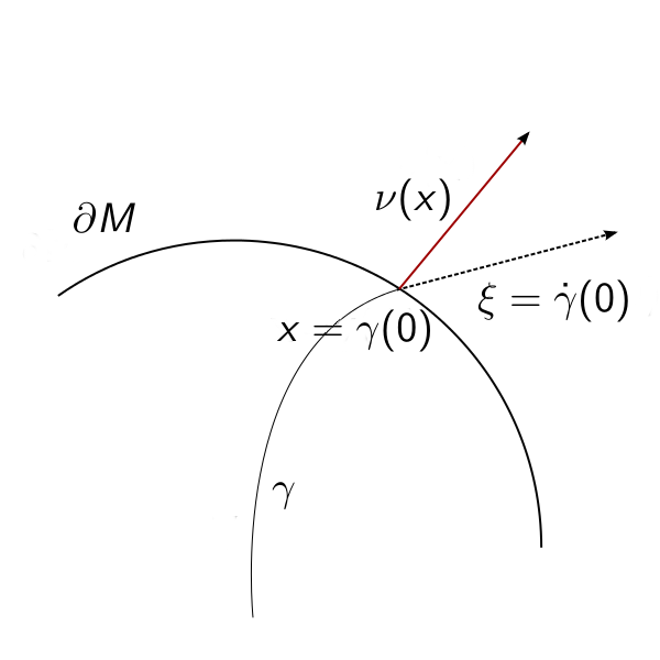
Fig. 2: In $x\in\partial M$ we have $\langle\xi,\nu(x)\rangle\geq 0$ (red arrow) at $\partial M$ and $\xi$ is the tangential vector (dotted arrow) in $x$. There is an “Outflow” with measured data $T(\gamma)=\int_{\gamma}n(y)\,dl(y)\geq 0$. In the case of an “Inflow”, $\langle\xi,\nu(x)\rangle<0$, the geodesic $\gamma$ would be outside from $M$ and hence $T(\gamma)=0$.

Definition 9 (Inflow, Outflow).

Let

$$\Omega M:=\left\{(x,\xi)\in TM:\|\xi\|_{g}^{2}:=g_{ij}(x)\xi^{i}\xi^{j}=1\right\}.$$

We call

$$\partial_{+}\Omega M:=\left\{(x,\xi)\in\Omega M:x\in\partial M,\langle\xi,\nu(x)\rangle\geq 0\right\}$$

Outflow and

$$\partial_{-}\Omega M:=\left\{(x,\xi)\in\Omega M:x\in\partial M,\langle\xi,\nu(x)\rangle<0\right\}$$

Inflow, where $\nu(x)$ is the outer normal at $M$ in $x$. We have

$$\partial\Omega M:=\partial_{+}\Omega M\cup\partial_{-}\Omega M$$

and $\partial_{\pm}\Omega M$ are compact manifolds.

The situation is illustrated in Figure 2. The following lemma is proven in [32].

Lemma 10 ([32, Lemma 4.1.1]).

Let $(M,g)$ be a compact, dissipative Riemannian manifold. Then the mapping $\tau_{-}:\partial_{+}\Omega M\to\mathbb{R}$ is a smooth function.

The data acquired by TOF measurements can now be modeled as integrals of $n$ along geodesics associated with the metric $g^{n}$. To this end let $n\in C^{\infty}(M)$ and $\gamma^{n}_{x,\xi}$ the solution of the geodesic equation (6) with respect to the metric $g^{n}$. The mapping $u^{meas}:\partial\Omega M\to\mathbb{R}^{+}$ with

(10) $$u^{meas}(x,\xi)=\begin{cases}0&\text{ if }(x,\xi)\in\partial_{-}\Omega M\\ \int_{\gamma^{n}_{x,\xi}}n(y)\,\mathrm{d}l(y)&\text{ if }(x,\xi)\in\partial_{+}\Omega M\\ \end{cases},$$

assigns a geodesic curve starting in $x\in\partial M$ with tangent $\xi\in T_{x}M$ its travel time until it leaves the domain. This is why we call $u^{meas}$ the TOF mapping. The inverse problem consists of computing the refractive index $n$ from $u^{meas}$. The forward operator is given by the ray transform

(11) $$R(n)(x,\xi):=\int_{\gamma^{n}_{x,\xi}}n(z)\,\mathrm{d}l(z),\qquad\mbox{for }(x,\xi)\in\partial_{+}\Omega M.$$

For $a\in C^{\infty}(M)$ we furthermore define the linearized ray transform

$$R_{a}(n)(x,\xi):=\int_{\gamma^{a}_{x,\xi}}n(z)\,dl,\qquad\forall(x,\xi)\in\partial_{+}\Omega M$$

where $\gamma^{a}_{x,\xi}$ is the solution of (6) with respect to the metric $g^{a}$ and initial values $\gamma^{a}_{x,\xi}(0)=x$ and $\dot{\gamma}^{a}_{x,\xi}(0)=\xi$. If $a=n$, we obviously have

$$R_{n}(n)=R(n).$$

The inverse problem of determining the refractive index $n$ from TOF measurements finally means to find a solution of

(12) $$R(n)=u^{meas}.$$

Note that the crucial point is that the curve along which $R$ integrates depends on the integrand $n$ turning (12) into a highly nonlinear, ill-posed problem.

2.4 Mathematical properties of $R$ and $R_{a}$

From now on we assume that the refractive index $n\in C^{\infty}(M)$ and $(M,g^{n})$ is a compact, dissipative Riemannian manifold (CDRM). We recall that this implies that for any two points $x,y\in M$ there exists a unique, maximal geodesic $\gamma$ connecting $x$ and $y$ which at the same time is the shortest path between these points. For proving the continuity of $R$ it is useful to introduce the phase function following the outlines of Guillemin and Sternberg [10]. Compare also [26, Section 2].
For $s\in\mathbb{R}$ and $\theta=(\cos\varphi,\sin\varphi)^{\top}\in S^{1}:=\{\theta\in\mathbb{R}^{2}:|\theta|=1\}$, $\varphi\in[0,2\pi)$, we denote by $\gamma_{\theta,s}:[\tau_{-},0]\to\mathbb{R}^{2}$ the unique solution of the geodesic equation (6) with respect to the refractive index $n$ and initial values

(13) $$\gamma_{\theta,s}(0)=r\theta+s\theta^{\perp}\text{ and }\dot{\gamma}_{\theta,s}(0)=\theta.$$

Here, $r>\mathrm{diam}(M)/2$ and $\tau_{-}<0$ is the unique parameter where $\gamma_{\theta,s}$ intersects the boundary $\partial M$ for the second time and $\theta^{\perp}=(-\sin\varphi,\cos\varphi)^{\top}\in S^{1}$ is perpendicular to $\theta$. The situation is illustrated in Figure 3. It is now possible to define $\gamma_{\theta,s}$ as level curves of a phase function $\Phi$.

Fig. 3: For a given direction $\theta\in S^{1}$ and $\theta^{\perp}\in S^{1}$ (red arrows) a point $x\in\mathbb{R}^{2}$ is defined by the two parameters $r,s\in\mathbb{R}$ (blue) such that $x=r\theta+s\theta^{\perp}$. The black curves represent geodesics passing $M$ initiating from the straight line $r\theta+\operatorname{span}{\theta^{\perp}}$ with vector of direction $\theta$.

Lemma 11 ([10, cf. Prop. 5.2]).

Let $g$ be a metric such that for $\theta\in S^{1}$ and $s,s^{\prime}\in\mathbb{R}$ with $s\neq s^{\prime}$ the geodesic curves $\gamma_{\theta,s}$ and $\gamma_{\theta,s^{\prime}}$ do not intersect. Then the matrix $\big{(}\partial_{t}\gamma_{\theta,s}(t),\partial_{s}\gamma_{\theta,s}(t)\big{)}$ is regular for fixed $\theta$ and there exists a phase function

$$\Phi:M\times S^{1}\to\mathbb{R},\qquad(y,\theta)\mapsto\Phi(y,\theta),$$

such that the geodesic $\gamma_{\theta,s}$ is implicitly given and uniquely determined by

$$\Phi\left(y,\theta\right)=s\quad\Longleftrightarrow\quad y\in\mathrm{Tr}(\gamma_{\theta,s}),\qquad s\in\mathbb{R}.$$

In that sense geodesic curves can be interpreted as manifolds of constant phase of a wave field.

Example 12.

Let $M:=\mathbb{B}:=\{x\in\mathbb{R}^{2}:|x|\leq 1\}$ and consider $(\mathbb{B},g_{0})$, i.e. the unit disk equipped with the Euclidean metric. Then the geodsics are straight lines and $\Phi:\mathbb{B}\times S^{1}\to\mathbb{R}$ is given by

$$\Phi(y,\theta)=\langle y,\theta^{\perp}\rangle$$

and $\Phi(y,\theta)=s$ is the usual parametrization of straight lines in parallel geometry. Here, $\theta=\theta(\varphi)=(\cos\varphi,\sin\varphi)^{\top}$ and $\theta^{\perp}=\theta(\varphi+\pi/2)=(-\sin\varphi,\cos\varphi)^{\top}$ for $\varphi\in[0,2\pi)$. Please note that by (13) the normal vector of a line is $\theta^{\perp}$ instead of $\theta$ as usual.

In Euclidean geometry (i.e. $n=1$) it is easy to determine the boundary intersection points $p,q\in\partial M$ of the straight line starting at $x\in M$ with vector of direction $\theta\in S^{1}$. For $n\not=1$ the situation is different. This is why we construct a so-called geodesic projection, a mapping which determines the intersection point with the boundary and the corresponding tangential vector of a geodesic curve that passes through $y\in M$.

Definition 13 (Geodesic projection).

Adopt the assumptions of Lemma 11. The mapping $\Pi:S^{1}\times\mathbb{R}\to\partial_{+}\Omega M$, given by

$$(\theta,s)\mapsto\Pi(\theta,s):=(x,\xi)\,,$$

where $(x,\xi)\in\partial_{+}\Omega M$ is uniquely determined by

$$(x,\xi)=\big{(}\gamma_{\theta,s}(\tau_{0}),\dot{\gamma}_{\theta,s}(\tau_{0})\big{)}\quad\mbox{with}\quad\tau_{0}=\max\big{\{}\gamma_{\theta,s}^{-1}\big{(}\mathrm{Tr}(\gamma_{\theta,s})\cap\partial M\big{)}\big{\}},$$

is called geodesic projection on the boundary $\partial_{+}\Omega M$.

The construction of $\Pi(\theta,s)_{1}=x$ is illustrated in Figure 4. The geodesic projection links the 2D parallel geometry in CT to the more general case of an inhomogeneous medium with given metric $g^{n}$; a fact which proves very useful for defining the backprojection operator and the implementation of our numerical solution approach for (12). Please note that we need the assumptions of Lemma 11 and the existence of a phase function that $\Pi$ is well-defined.

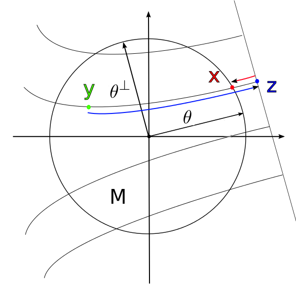
Fig. 4: Illustration of the first component of the geodesic projection $\Pi_{1}$. At first the green point $y\in M$ is mapped by $\Phi$ (blue arrow) on $z=\Phi(y,\theta)\theta^{\perp}+r\theta$ (blue point) and subsequently it is mapped to the boundary $x\in\partial M$ (red point).

If $a\in C^{\infty}(M)$ generates a metric $g^{a}$ which is dissipative, then the linearized operator $R_{a}$ is continuous.

Theorem 14 (Th. 4.2.1 from [32]).

Let $a\in C^{\infty}(M)$ such that the corresponding metric $g^{a}_{ij}=a^{2}\delta_{ij}$ turns $(M,g^{a})$ into a CDRM. Then, the linearized ray transform $R_{a}:L^{2}(M)\to L^{2}(\partial_{+}\Omega M)$ is continuous.

Under the assumption that the functions $a$ generating dissipative metrics $g^{a}$ are dense in $L^{2}(M)$, then we even can prove the continuity of the nonlinear operator $R$.

Theorem 15.

Suppose that the subset

$$\mathcal{M}:=\big{\{}a\in L^{2}(M)\cap C^{\infty}(M):(M,g^{a})\mbox{is a CDRM}\big{\}}$$

is dense in $L^{2}(M)$. Then $R:\mathcal{D}(R):=L^{2}(M)\cap C^{\infty}(M)\to L^{2}(\partial_{+}\Omega M)$ is continuous.

Proof.

Let $a\in\mathcal{D}(R)$ be arbitrary and $\{a_{k}\}\subset\mathcal{M}$ be a sequence in $\mathcal{M}$ such that $a_{k}\to a$ as $k\to\infty$. Then we can estimate

$$\left\|R(a)-R(a_{k})\right\|_{L^{2}(\partial_{+}\Omega M)}$$

$$= \left\|R(a)-R_{a_{k}}(a)+R_{a_{k}}(a)-R(a_{k})\right\|_{L^{2}(\partial_{+}\Omega M)}$$

$$\leq \left\|R(a)-R_{a_{k}}(a)\right\|_{L^{2}(\partial_{+}\Omega M)}+\left\|R_{a_{k}}(a-a_{k})\right\|_{L^{2}(\partial_{+}\Omega M)}.$$

Since $a_{k}\in\mathcal{M}$ we have that $R_{a_{k}}$ is linear and continuous due to Theorem 14 and thusly

$$\left\|R_{a_{k}}(a-a_{k})\right\|_{L^{2}(\partial_{+}\Omega M)}\leq\|R_{a_{k}}\|_{L^{2}(M)\to L^{2}(\partial_{+}\Omega M)}\left\|a-a_{k}\right\|_{L^{2}(M)}.$$

To tackle the first term we assume $\gamma_{x,\xi}^{a}(t)$, $\gamma_{x,\xi}^{a_{k}}(t)$ to be respective solutions of the geodesic equation (6) parametrized on $t\in[0,1]$. We obtain

$$\left\|R(a)-R_{a_{k}}(a)\right\|_{L^{2}(\partial_{+}\Omega M)}$$

$$= \left\|\int_{\gamma^{a}_{x,\xi}}a(z)\,\mathrm{d}l(z)-\int_{\gamma^{a_{k}}_{x,\xi}}a(z)\,\mathrm{d}l(z)\right\|_{L^{2}(\partial_{+}\Omega M)}$$

$$= \left\|\int_{0}^{1}a(\gamma^{a}_{x,\xi}(t))|\dot{\gamma}^{a}_{x,\xi}(t)|\,\mathrm{d}t-\int_{0}^{1}a(\gamma^{a_{k}}_{x,\xi}(t))|\dot{\gamma}^{a_{k}}_{x,\xi}(t)|\,\mathrm{d}t\right\|_{L^{2}(\partial_{+}\Omega M)}$$

$$\leq \sup_{y\in M}|a(y)|\,\left\|\int_{0}^{1}|\dot{\gamma}^{a}_{x,\xi}(t)-\dot{\gamma}^{a_{k}}_{x,\xi}(t)|\,\mathrm{d}t\right\|_{L^{2}(\partial\Omega M)}.$$

Let $\varepsilon>0$ be arbitrary. For $k$ sufficiently large we deduce from Lemma 6 and Lemma 10

$$\sup_{(x,\xi)\in TM}\sup_{t\in[0,1]}\|\dot{\gamma}^{a}_{x,\xi}(t)-\dot{\gamma}^{a_{k}}_{x,\xi}(t)\|<\frac{\varepsilon}{2\sup_{y\in M}|a(y)|}.$$

A sufficiently large $k$ furthermore assures that

$$\|a-a_{k}\|_{L^{2}(M)}<\big{(}2\|R_{a_{k}}\|_{L^{2}(M)\to L^{2}(\partial_{+}\Omega M)}\big{)}^{-1}\,\varepsilon.$$

Putting all this together we conclude

$$\left\|R(a)-R(a_{k})\right\|_{L^{2}(\partial_{+}\Omega M)} \leq \left\|R(a)-R_{a_{k}}(a)\right\|_{L^{2}(\partial_{+}\Omega M)}+\left\|R_{a_{k}}(a-a_{k})\right\|_{L^{2}(\partial_{+}\Omega M)}$$

$$\leq \varepsilon/2+\varepsilon/2=\varepsilon$$

if only $k$ is sufficiently large. This proves the theorem. ∎

Unfortunately by now there is no proof that $\mathcal{M}$ is dense in $L^{2}(M)$ or not.
For completeness we give two existence and uniqueness results which can be found in [33].

Theorem 16 (Th. 1.1.1 and Th. 1.2.1 from [33]).

Let $a\in C^{\infty}(M)$ such that it induces a simple Riemannian metric.

• If the measured data $u^{meas}$ is generated by a refractive index $n\in C^{2}(M)$, then the operator equation

  $$u^{meas}=R_{a}n$$

  has a unique solution $n\in L^{2}(M)\cap C^{2}(M)$.

• If the measured data $u^{meas}$ is generated by a refractive index $n\in C^{4}(M)$, then the nonlinear operator equation

  $$u^{meas}=R(n)$$

  has a unique solution $n\in L^{2}(M)\cap C^{4}(M)$.
  

2.5 The method of characteristics

Our numerical solution scheme for (12) is iterative and demands for evaluating the forward operator, i.e. the computation of the TOF measurements for a given metric, in each iteration step. We do this using the fact that the TOF function $u$ (9) satisfies a partial differential equation where the differential operator is the so called geodesic vector field.

Definition 17 (Geodesic flow).

Let $(M,g)$ be a Riemannian manifold and $u:T^{0}M\to\mathbb{R}^{+}$ the TOF mapping (9) . We call $Hu:T^{0}M\to\mathbb{R}$ defined by

$$Hu(x,\xi):=\xi^{i}\frac{\partial u}{\partial x^{i}}-\Gamma^{i}_{jk}(x)\xi^{j}\xi^{k}\frac{\partial u}{\partial\xi^{i}}\text{, for all }(x,\xi)\in T^{0}M,$$

geodesic vector field.

There s a fundamental connection between the geodesic vector field and the refractive index regarding our measure geometry.

Theorem 18.

Let $(M,g)$ be a Riemannian manifold with the metric tensor given as $g_{ij}(x)=g^{n}_{ij}=n^{2}(x)\delta_{ij}$. Then for all $(x,\xi)\in T^{0}M$ the transport equation

$$Hu(x,\xi)=n(x)$$

holds true.

Proof.

A proof can be found in [32, Section 1.2]. ∎

Remark 19.

The differential operator

$$H=\xi^{i}\frac{\partial}{\partial x^{i}}-\Gamma^{i}_{jk}\xi^{j}\xi^{k}\frac{\partial}{\partial\xi^{i}}$$

has a specific geometrical meaning. Let $G(t;\cdot,\cdot):TM\to TM$ be the solution of

$$G^{\prime}(t;x,\xi)=H(G(t;x,\xi))\,,\qquad G(0;x,\xi)=(x,\xi)\,.$$

Then we have

$$G(t;x,\xi)=\left(\gamma_{x,\xi}(t),\dot{\gamma}_{x,\xi}(t)\right)$$

for a geodesic $\gamma_{x,\xi}$. This is the geodesic flow associated with the vector field $H$.

Corollary 20.

Let $n\in C^{\infty}(M)$ be positive and the metric $g$ on $M$ defined by

$$g^{n}(x)=g_{ij}^{n}(x)dx^{i}\,dx^{j}$$

with metric tensor

$$g_{ij}^{n}(x)=n^{2}(x)\delta_{ij}.$$

Then

(14) $$Hu(x,\xi) = \xi^{i}\frac{\partial u}{\partial x^{i}}(x,\xi)+n^{-1}(x)\left(\frac{\partial n}{\partial x^{i}}(x)\|\xi\|^{2}-2\xi^{i}\langle\xi,\nabla n(x)\rangle\right)\frac{\partial u}{\partial\xi^{i}}(x,\xi)$$

$$= n(x)$$

holds true for all $(x,\xi)\in T^{0}M$.

Proof.

Let $(x,\xi)\in T^{0}M$. For $i=1$ the Christoffel symbols are given by

$$\left(\Gamma^{1}_{ij}(x)\right)_{i,j=1}^{2}=n^{-1}(x)\begin{pmatrix}\frac{\partial n(x)}{\partial x_{1}}&\frac{\partial n(x)}{\partial x_{2}}\\ \frac{\partial n(x)}{\partial x_{2}}&-\frac{\partial n(x)}{\partial x_{1}}\end{pmatrix}.$$

For the partial derivatives we have

$$\Gamma^{1}_{jk}(x)\xi^{j}\xi^{k} = n^{-1}(x)\begin{pmatrix}\xi_{1}&\xi_{2}\end{pmatrix}\begin{pmatrix}\frac{\partial n(x)}{\partial x_{1}}&\frac{\partial n(x)}{\partial x_{2}}\\ \frac{\partial n(x)}{\partial x_{2}}&-\frac{\partial n(x)}{\partial x_{1}}\end{pmatrix}\begin{pmatrix}\xi_{1}\\ \xi_{2}\end{pmatrix}$$

$$= n^{-1}(x)\left(\frac{\partial n(x)}{\partial x_{1}}\xi_{1}^{2}+2\frac{\partial n(x)}{\partial x_{2}}\xi_{1}\xi_{2}-\frac{\partial n(x)}{\partial x_{1}}\xi_{2}^{2}\right)$$

$$= n^{-1}(x)\left(2\frac{\partial n(x)}{\partial x_{1}}\xi_{1}^{2}+2\frac{\partial n(x)}{\partial x_{2}}\xi_{1}\xi_{2}-\frac{\partial n(x)}{\partial x_{1}}\|\xi\|^{2}\right)$$

$$= n^{-1}(x)\left(2\xi_{1}\left[\xi_{1}\frac{\partial n(x)}{\partial x_{1}}+\xi_{2}\frac{\partial n(x)}{\partial x_{2}}\right]-\frac{\partial n(x)}{\partial x_{1}}\|\xi\|^{2}\right)$$

$$= n^{-1}(x)\left(2\xi_{1}\langle\xi,\nabla n(x)\rangle-\frac{\partial n(x)}{\partial x_{1}}\|\xi\|^{2}\right).$$

In the same way we compute

$$\Gamma^{2}_{jk}(x)\xi^{j}\xi^{k}=n^{-1}(x)\left(2\xi_{2}\langle\xi,\nabla n(x)\rangle-\frac{\partial n(x)}{\partial x_{2}}\|\xi\|^{2}\right)$$

and the proposition follows immediately. ∎

Remark 21.

In Theorem 18 we transformed the inverse problem (12) into a parameter identification problem for the transport equation with boundary conditions (10). Again we recognize that the problem is highly nonlinear, because the refractive index $n$ appears as source-term as well as parameter in the differential operator.

According to the transport equation (14) we want to develop a method to compute the geodesic curves for a given refractive index. To this end we use the method of characteristics. Let $\operatorname{Graph}(u):=\left\{\left(x,\xi,u(x,\xi)\right):(x,\xi)\in TM\right\}$ be the graph of $u$ and

$$\left(x(t),\xi(t),z(t)\right):=\left(x(t),\xi(t),u\left(x(t),\xi(t)\right)\right)$$

a curve in $\operatorname{Graph}(u)$ with $t\in I$, $I$ a compact interval. Differentiating with respect to $t$ yields

$$\left(\dot{x}(t),\dot{\xi}(t),\dot{z}(t)\right)=\left(\dot{x}(t),\dot{\xi}(t),\frac{\partial u(x(t),\xi(t))}{\partial x^{i}}\dot{x}^{i}(t)+\frac{\partial u(x(t),\xi(t))}{\partial\xi^{i}}\dot{\xi}^{i}(t)\right).$$

Then $\left(\nabla_{x}u(x(t),\xi(t)),\nabla_{\xi}u(x(t),\xi(t)),-1\right)$ is a normal of the curve at $t$ since

$$\begin{pmatrix}\nabla_{x}u(x(t),\xi(t))\\ \nabla_{\xi}u(x(t),\xi(t))\\ -1\end{pmatrix}\left(\dot{x}(t),\dot{\xi}(t),\frac{\partial u(x(x(t),\xi(t))}{\partial x^{i}}\dot{x}^{i}(t)+\frac{\partial u(x(x(t),\xi(t))}{\partial\xi^{i}}\dot{\xi}^{i}(t)\right)$$

$$= \nabla_{x}u(x(t),\xi(t))\cdot\dot{x}(t)+\nabla_{\xi}u(x(t),\xi(t))\cdot\dot{\xi}(t)-\frac{\partial u(x(t),\xi(t))}{\partial x^{i}}\dot{x}^{i}(t)$$

$$-\frac{\partial u(x(t),\xi(t))}{\partial\xi^{i}}\dot{\xi}^{i}(t)$$

$$= 0.$$

From $Hu=n$ we get that $\big{(}\xi(t),\big{(}-\Gamma^{i}_{jk}(x(t))\xi^{j}(t)\xi^{k}(t)\big{)}_{i},n(x(t))\big{)}$ is a tangent vector, because

$$\begin{pmatrix}\nabla_{x}u(x(t),\xi(t))\\ \nabla_{\xi}u(x(t),\xi(t))\\ -1\end{pmatrix}\left(\xi(t),\left(-\Gamma^{i}_{jk}(x(t))\xi^{j}(t)\xi^{k}(t)\right)_{i},n(x(t))\right)$$

$$= \xi\cdot\nabla_{x}u(x(t),\xi(t))-\Gamma^{i}_{jk}(x(t))\xi^{i}(t)\xi^{j}(t)\frac{\partial u(x(t),\xi(t))}{\partial\xi^{i}}-n(x(t))$$

$$= Hu(x(t),\xi(t))-n(x(t))$$

$$= 0.$$

If we choose a boundary point $x_{0}\in\partial M$ and a direction $0\not=\xi_{0}\in T_{x_{0}}M$, we finally obtain the initial value problem

(15) $$\text{(IVP)}\begin{cases}\dot{x}_{i}(t)=\xi_{i}(t)&\text{ for }t\in I,\,i=1,2\\ \dot{\xi}_{i}(t)=-\Gamma^{i}_{jk}(x(t))\xi^{j}(t)\xi^{k}(t)&\text{ for }t\in I,\,i=1,2\\ \dot{z}(t)=n(x(t))&\text{ for }t\in I\\ &\\ x(0)=x_{0}&\\ \xi(0)=\xi_{0}&\\ z(0)=0&\end{cases}.$$

The solution is a characteristic, i.e. a curve on $\operatorname{Graph}(u)$, which is the union of all characteristics. But the characteristic curves of $H$ are just the geodesics of $(M,g^{n})$. Solving (15) thus follows a geodesic curve starting at the boundary until it meets $\partial M$ again say at $t=t_{1}$. Then $z(t_{1})$ is the TOF of the ultrasound signal propagating from $x_{0}$ in direction $\xi_{0}$ until it leaves the boundary $\partial M$ at $x(t_{1})$.

3 A regularization method for (12)

We intend to solve the nonlinear inverse problem (12) iteratively by a steepest descent method for a Tikhonov functional where we use the linearized operator $R_{a}$. In a first subsection we define this functional, the iteration scheme and some of its properties. The second subsection then is devoted to deal with implementation issues of this method.

3.1 The Tikhonov functional and its minimization

Again we assume $M\subset\mathbb{R}^{2}$ to be compact. For $1\leq p<\infty$ and $\alpha>0$ we consider the Tikhonov functional $J_{\alpha}:X_{p}:=L^{p}(M)\cap C^{\infty}(M)\to\mathbb{R}$ defined by

(16) $$J_{\alpha}(f)=\frac{1}{2}\|R(f)-u^{meas}\|_{Y}^{2}+\frac{\alpha}{p}\|f-1\|_{L^{p}(M)}^{p}.$$

Here we used the notation $Y:=L^{2}(\partial_{+}\Omega M)$. The penalty term $\frac{1}{p}\|f-1\|_{L^{p}(M)}^{p}$ thereby ensures that the solution gives a refractive index that does not vary too strongly from $n=1$, i.e. a homogeneous medium. This is a supposed a priori information about the exact solution which we want to incorporate. Furthermore this term of course yields stability of the solution process. The choice $p=1$ furthermore allows also for sparse solutions. Because of the nonlinearity we can not expect that there exists a unique minimizer of $J_{\alpha}(f)\leadsto\min$. Usually a stationary point $f^{*}$ of $J_{\alpha}$ is searched by the condition $0\in\partial J_{\alpha}(f^{*})$. There we face a further problem: the computation of a Gâteaux derivative $R^{\prime}(f)$ of $R$. The computation is still object of current research. This is why we linearize the problem by using $R_{a}$ for fixed $a\in X_{p}$ instead of the nonlinear operator $R$. In this way a second Tikhonov functional $J_{\alpha}^{a}:L^{p}(M)\to\mathbb{R}$ comes up which is defined by

$$J_{\alpha}^{a}(f)=\frac{1}{2}\|R_{a}(f)-u^{meas}\|_{Y}^{2}+\frac{\alpha}{p}\|f-1\|_{L^{p}(M)}^{p}$$

with $a\in C^{\infty}(M)$ fixed. Since $R_{a}$ is linear, it is simple to compute the subdifferential $\partial J_{\alpha}^{a}$. The last ingredient we need for doing so is the adjoint $R_{a}^{*}$ of $R_{a}$.

Lemma 22.

Let $a\in C^{\infty}(M)$ be fixed. Then the adjoint operator $R^{*}_{a}:Y\to L^{p^{*}}(M)$ is given by

(17) $$R_{a}^{*}\omega(y)=\int_{S^{1}}\omega\big{(}\Pi(\theta,\Phi(y,\theta))\big{)}\,\Big{|}\mathrm{det}\frac{\partial}{\partial(\theta,s)}\Pi\big{(}\theta,\Phi(y,\theta)\big{)}\Big{|}\,\mathrm{d}\theta\,,\qquad y\in M,$$

where $\Pi:S^{1}\times[-r,r]\to\partial_{+}\Omega M$ is the geodesic projection from Definition 13,

$$\mathrm{det}\frac{\partial}{\partial(\theta,s)}\Pi\big{(}\theta,\Phi(y,\theta)\big{)}$$

denotes the Jacobian of $\Pi(\theta,s)$ evaluated at $s=\Phi(y,\theta)$, $r=\mathrm{diam}(M)/2$ and $p^{*}$ satisfies $(p^{*})^{-1}+p^{-1}=1$ for $p\in(1,\infty)$ and $p^{*}=\infty$ for $p=1$.

Proof.

Let $f\in L^{p}(M)$ and $\omega\in Y$. Then we have

$$\langle R_{a}f(x,\xi),\omega(x,\xi)\rangle_{Y} = \int_{\partial_{+}\Omega M}R_{a}f(x,\xi)\omega(x,\xi)\,\mathrm{d}x\wedge\mathrm{d}\xi$$

$$=\int_{\partial_{+}\Omega M}\int_{\gamma^{a}_{x,\xi}}f(z)\omega(x,\xi)\,\mathrm{d}l(z)\,\mathrm{d}x\wedge\mathrm{d}\xi$$

$$=\int_{S^{1}}\int_{-r}^{r}\int_{M}f(y)\delta\big{(}s-\Phi(y,\theta)\big{)}\omega\big{(}\Pi(\theta,s)\big{)}\,\mathrm{d}y\,\Big{|}\mathrm{det}\frac{\partial}{\partial(\theta,s)}\Pi(\theta,s)\Big{|}\,\mathrm{d}s\,d\theta$$

$$=\int_{M}f(y)\int_{S^{1}}\int_{-r}^{r}\omega\big{(}\Pi(\theta,s)\big{)}\delta\big{(}s-\Phi(y,\theta)\big{)}\,\Big{|}\mathrm{det}\frac{\partial}{\partial(\theta,s)}\Pi(\theta,s)\Big{|}\,\mathrm{d}s\,\mathrm{d}\theta\,\mathrm{d}y$$

$$=\int_{M}f(y)\int_{S^{1}}\omega\big{(}\Pi(\theta,\Phi(y,\theta))\big{)}\,\Big{|}\mathrm{det}\frac{\partial}{\partial(\theta,s)}\Pi\big{(}\theta,\Phi(y,\theta)\big{)}\Big{|}\,\mathrm{d}\theta\,dy$$

$$=\langle f,R_{a}^{*}\omega\rangle_{L^{p}\times L^{p^{*}}}.$$

∎

Note that $R_{a}^{*}$ is an analogon to the classical backprojection operator, since it integrates along all geodesics passing a given point $y\in M$. The numerical approximation of the geodesic projection $\Pi(\theta,\Phi(y,\theta))$ will prove the part of our method which is most time consuming.

Example 23.

Consider again the 2D parallel geometry in the unit disk $M=\mathbb{B}$, equipped with the Euclidean geometry $g_{0}$. Then the geodesics are straight lines and the geodesic projection $\Pi:S^{1}\times(-1,1)\to\partial_{+}\Omega\mathbb{B}$ is given by

$$\Pi(\theta,s)=(x,\xi)=(s\theta+\sqrt{1-s^{2}}\theta^{\perp},\theta^{\perp}),$$

where $\theta=\theta(\varphi)=(\cos\varphi,\sin\varphi)^{\top}$, $\theta^{\perp}=\theta(\varphi+\pi/2)=(-\sin\varphi,\cos\varphi)^{\top}$. In that sense we can equivalently formulate $\Pi$ as mapping $\Pi:[0,2\pi)\times(-1,1)\to[0,2\pi)\times[0,2\pi)$ by

$$\Pi(\varphi,s)=\Big{(}\varphi+\arccos s,\big{(}\varphi+\frac{\pi}{2}\big{)}\,\mathrm{mod}\,2\pi\Big{)}$$

and obtain

$$\Big{|}\mathrm{det}\frac{\partial}{\partial(\theta,s)}\Pi(\theta,s)\Big{|}=\frac{1}{\sqrt{1-s^{2}}}.$$

Since in $(\mathbb{B},g_{0})$ the phase function is given as $\Phi(y,\theta)=\langle y,\theta^{\perp}\rangle$, we obtain the usual backprojection operator in $(\mathbb{B},g_{0})$

$$R^{*}\omega(y)=\int_{S^{1}}\omega\big{(}\Pi(\theta,\langle y,\theta\rangle)\big{)}\,\frac{\mathrm{d}\theta}{\sqrt{1-\langle y,\theta\rangle^{2}}}.$$

Note that in the last identity we substituted $\theta^{\perp}$ by $\theta$ to stick on the conventional notation. The weight $(1-\langle y,\theta\rangle^{2})^{-1/2}$ comes from the fact that the lines $\ell(x,\xi)$ here are parametrized by a boundary point $x\in\partial\mathbb{B}$ and a unit tangential vector $\xi$ in $x$ with $\langle\xi,x\rangle\geq 0$ instead of the conventional parametrization by a normal vector $\theta$ and offset $s\in\mathbb{R}$.

If we would just minimize $J_{\alpha}^{a}$ for fixed $a$ we would completely neglect the influence of the integrand $f$ to the integration curves. Thus the idea of our algorithm is to use a steepest descent method which uses the actual iterate $n_{k-1}$ to compute the new one $n_{k}$ by minimizing $J_{\alpha}^{n_{k-1}}$. This of course means to compute a new set of geodesic curves in each iteration step. This leads to the following, adaptive iteration scheme.

Algorithm 24 (Iterative, adaptive minimization method).

Input: initial value $n_{0}$, sequence of regularization parameters $\alpha=\left(\alpha_{k}\right)_{k=1,2,\ldots}\subset\mathbb{R}^{+}$.

• Compute for $n_{0}$ the set of geodesics $\mathcal{G}_{0}=\mathcal{G}_{n_{0}}$ and set $J_{\alpha_{0}}^{0}(n_{0})=J_{\alpha_{0}}^{n_{0}}(n_{0})$.

• Repeat for $k=1,2,\ldots$

  • Minimize $J_{\alpha}^{n_{k-1}}$, i.e. compute

    $$n_{k}:=\arg\min_{f\in L^{p}(M)}J_{\alpha_{k-1}}^{n_{k-1}}(f).$$

  • Compute the new set of geodesics $\mathcal{G}_{k}:=\mathcal{G}_{n_{k}}$ and evaluate $J_{\alpha_{k}}^{k}(n_{k})=J_{\alpha_{k}}^{n_{k}}(n_{k})$.

Output: $n_{k^{*}}$ for a stopping index $k^{*}$, set of geodesics $\mathcal{G}_{k^{*}}$.

The minimization step (S1a) is done iteratively using the Landweber method, compare e.g. [31]. Let $n_{k}$ be the actual iterate in step (S1), then this iteration reads as

$$n_{k}^{0} = n_{k}$$

$$n_{k}^{l+1} = n_{k}^{l}-\mu_{l}\left(A_{k}^{*}(A_{k}n_{k}^{l}-u^{meas})+\frac{\alpha_{k}}{p}n_{k,l}^{*}\right),\qquad l=0,1,2,\ldots$$

$$n_{k+1} = n_{k}^{l^{*}}$$

with an element $n_{k,l}^{*}\in\partial(\|n_{k}^{l}-1\|_{L^{p}(M)}^{p})\subset L^{p^{*}}(M)$, $A_{k}:=R_{n_{k}}$, regularization parameter $\alpha_{k}>0$, step size $\mu_{l}>0$, $l=0,1,\ldots$ and reasonable stopping index $l^{*}\in\mathbb{N}$. For $1<p<\infty$ we have

$$\partial\left(\|n_{k}^{l}-1\|_{L^{2}(M)}^{p}\right)=p\|n_{k}^{l}-1\|_{L^{p}(M)}^{p-2}\cdot(n_{k}^{l}-1).$$

for $n_{k}^{l}\in L^{p}(M)$. For $p=1$ we use the standard soft threshold algorithm from [8]. This yields the following version of step (S1) from Algorithm 24 as it is implemented.

Algorithm 25 (Steepest descent method for $J_{\alpha_{k}}^{n_{k}}$).

Input: Current iterate $n_{k}$, regularization parameter $\alpha_{k}>0$.

• Define the operator $R_{k}:=R_{n_{k}}$ and its adjoint $R^{*}_{k}=R^{*}_{n_{k}}$ by (17).

• Set $n_{k}^{0}:=n_{k}$ and iterate for $l=0,1,2,\ldots,l^{*}$

  • Compute the residuum $r^{l-1}=R_{k}n_{k}^{l-1}-u^{meas}$ and stop if $\|r^{l-1}\|_{Y}=0$.

  • Evaluate the adjoint operator $r_{*}^{l-1}=R^{*}_{k}r^{l-1}$.

  • Determine a new search direction by

    $$\Delta^{l-1}=r_{*}^{l-1}+\alpha_{k}\|n_{k}^{l-1}-1\|_{L^{p}(M)}^{p-2}\cdot(n_{k}^{l-1}-1)$$

    in case $1<p<\infty$ or use soft thresholding for $p=1$.

  • Choose a decent step size $\mu_{l-1}>0$ and update

    $$n_{k}^{l}:=n_{k}^{l-1}-\mu_{l-1}\Delta^{l-1}.$$

• Set $n_{k+1}=n_{k}^{l^{*}}$.

Output: new iterate $n_{k+1}$.

Remark 26.

• The evaluation of the linearized forward operator $R_{k}$ in step (S1a) is computed quickly and depends on the discretization of the geodesics and the evaluation of $n_{k}$.

• The computation of the adjoint in step (S1b) however is very time consuming. The difficulty lies in the interpolation of the geodesics. The challenge is to find the geodesics that pass through a point $y\in M$, emitted from a direction $\xi\in T\partial M$ at the boundary.

• The step size $\mu_{l}>0$ in step (S1d) can be determined by a line-search algorithm.

• For convergence of the Landweber method in Algorithm 25 to the minimum norm solution we refer to [30, 31].

Our aim is to prove that Algorithms 24, 25 generate a sequence of iterates $\{n_{k}\}$ of decreasing values $J_{\alpha}(n_{k})$ for the Tikhonov functional $J_{\alpha}$ (16). To this end we define the mapping $\mathcal{T}:L^{p}(M)\to L^{p}(M)$ by

$$a\mapsto\arg\min_{f\in L^{p}(M)}J^{a}_{\alpha}(f)=\arg\min_{f\in L^{p}(M)}\left\{\frac{1}{2}\left\|R_{a}f-u^{meas}\right\|_{L^{p}(M)}^{2}+\frac{\alpha}{p}\left\|f-1\right\|_{L^{p}(M)}^{p}\right\}.$$

Agorithm 24 reads then as

(18) $$n_{k+1}:=\mathcal{T}(n_{k})=\arg\min_{f\in L^{p}(M)}J^{n_{k}}_{\alpha}(f)$$

with given initial value $n_{0}\in L^{p}(M)$. Assuming that $\mathcal{T}$ is a contraction, then Banach’s fixed point theorem says that $\{n_{k}\}$ converges to a unique $n^{*}$ satisfying

$$n^{*}=\mathcal{T}(n^{*}).$$

Lemma 27.

Let $\mathcal{T}:L^{p}(M)\to L^{p}(M)$ be a contraction and $n^{*}$ be the unique fixed point of $\mathcal{T}$ in $L^{p}(M)$. Then $n^{*}=\lim_{k\rightarrow\infty}n_{k}$ and

$$J_{\alpha}(n^{*})\leq J_{\alpha}^{n^{*}}(f)$$

holds true for all $f\in L^{p}(M)$ and $\alpha>0$.

Proof.

Since

$$n^{*}=\mathcal{T}(n^{*})=\arg\min_{f\in L^{p}(M)}J^{n^{*}}_{\alpha}(f),$$

we have

$$J_{\alpha}(n^{*})=J^{n^{*}}_{\alpha}(n^{*})\leq J^{n^{*}}_{\alpha}(f)$$

for all $f\in L^{p}(M)$. ∎

Note that in general we do not have

(19) $$J_{\alpha}(n^{*})\leq J_{\alpha}^{a}(n^{*})\text{ for all }a\in X_{p}$$

but assuming that (19) holds at least in a neighborhood of $n^{*}$, then Algorithm (24) in fact generates a decreasing sequence $J_{\alpha}(n^{k})$.

Lemma 28.

Let $\{n_{k}\}_{k=0,1,\ldots}$ be the sequence of iterates generated by Algorithm 24. We assume that there exists a $k^{*}\in\mathbb{N}$ such that

$$J_{\alpha}(n_{k})\leq J_{\alpha}^{a}(n_{k})\qquad\mbox{for all }a\in X_{p}$$

whenever $k\geq k^{*}$. Then for $k\geq k^{*}$ the Tikhonov functional $J_{\alpha}(n_{k})$ is monotonically decreasing, we have

$$J_{\alpha}(n_{k+1})\leq J_{\alpha}(n_{k}),$$

for all $k\geq k^{*}$.

Proof.

According to the assumptions for $k\geq k^{*}$ we have

$$J_{\alpha}(n_{k+1})\leq J_{\alpha}(n_{k+1})+\left(J_{\alpha}^{n_{k}}(n_{k+1})-J_{\alpha}(n_{k+1})\right)=J_{\alpha}^{n_{k}}(n_{k+1})\leq J_{\alpha}^{n_{k}}(n_{k})=J_{\alpha}(n_{k}),$$

because $n_{k+1}$ is a minimizer of $J_{\alpha}^{n_{k}}$.
∎

Summarizing we found a criterion for the iteration sequence $\{n_{k}\}$ to have a weak limit point.

Theorem 29.

Adopt the assumptions of Lemma 28. Then the sequence of iterates $\{n_{k}\}$ generated by Algorithm 24 has a weakly convergent subsequence, if $1<p<\infty$.

Proof.

Lemma 28 shows that the sequence $J_{\alpha}(n_{k})$ is monotonically decreasing and hence converging, since it is bounded from below. Thus $\{J_{\alpha}(n_{k})\}$ is bounded. Because

$$\frac{\alpha}{p}\|n_{k}-1\|_{L^{p}(M)}^{p}\leq J_{\alpha}(n_{k}),$$

the sequence $\{n_{k}\}$ is bounded, too. The spaces $L^{p}(M)$ are reflexive for $1<p<\infty$ which implies that $\{n_{k}\}$ has a weakly convergent subsequence.
∎

3.2 Implementation of Algorithms 24, 25

In this subsection we address issues of the implementation of the Algorithms 24 and 25. For simplicity we set $M:=\mathbb{B}$, the closed unit disk in $\mathbb{R}^{2}$.
At first we describe the discretization of $M$ and $n$. Let $n\in L^{p}(\mathbb{R}^{2})\cap C^{\infty}(\mathbb{R}^{2})$. For a given discretization step size $h>0$ we define the equally spaced grid

(20) $$E^{h}:=\left\{(r_{i},s_{j})\in\mathbb{R}^{2}:r_{i}=ih,\,s_{j}=jh,\,\forall i,j\in\mathbb{Z}\right\}\subset\mathbb{R}^{2}.$$

and $e_{ij}^{h}\subset\mathbb{R}^{2}$ by

$$e_{ij}^{h}:=\left\{(r,s)\in\mathbb{R}^{2}:r_{i}\leq r<r_{i+1},\,s_{j}\leq s<s_{j+1},\,(r_{i},s_{j}),(r_{i+1},s_{j+1})\in E^{h}\right\}$$

for $i,j\in\mathbb{Z}$. On $E^{h}$ we define the grid values $F^{h}(n)$ of $n$ by

$$F^{h}(n):=\left\{n_{ij}=n(r_{i},s_{j}):(r_{i},s_{j})\in E^{h}\right\}$$

and bilinear functions $\varphi_{ij}^{n}:\mathbb{R}^{2}\to\mathbb{R}$ by

$$\varphi_{ij}^{n}(r,s) =$$

$$\begin{cases}F^{h}_{ij}(n)+\frac{r-r_{i}}{h}\left(F^{h}_{i+1,j}(n)-F^{h}_{i,j}(n)\right)+\frac{s-s_{j}}{h}\left(F^{h}_{i,j+1}(n)-F^{h}_{i,j}(n)\right)&\\ \,+\frac{(r-r_{i})(s-s_{j})}{h^{2}}\left(F^{h}_{i+1,j+1}(n)-F^{h}_{i+1,j}(n)-F^{h}_{i,j+1}(n)+F^{h}_{i,j}(n)\right)&\text{ for }(r,s)\in e_{ij}^{h}\\ 0&\text{ otherwise}\end{cases}.$$

The unique bilinear interpolate $n^{h}:\mathbb{R}^{2}\to\mathbb{R}$ of $n$ is then given by

$$n^{h}(r,s):=\sum_{i,j\in\mathbb{Z}}\varphi_{ij}^{n}(r,s).$$

The set of all piecewise bilinear interpolates is denoted by

$$V^{h}:=\Big{\{}n^{h}(r,s):=\sum_{i,j\in\mathbb{Z}}\varphi_{ij}^{n}(r,s):n\in X_{p}\Big{\}}.$$

The following properties of $n$ and its interpolate $n^{h}$ are obvious:

• $n(r_{i},s_{j})=n^{h}(r_{i},s_{j})$ for all $(r_{i},s_{j})\in E^{h}$
  

• $n^{h}$ ist continuous on every element $e_{ij}^{h}$ and differentiable in the interior of $e_{ij}^{h}$
  

Remark 30.

For numerical purposes we cover the unit disk $M$ by a subset of the grid $\tilde{E}^{h}:=E^{h}\cap[-1,1]\times[-1,1]$ and set $h=1/Q$ for an integer $Q\in\mathbb{N}$. For the number of grid points we have $|\tilde{E}^{h}|=(2Q+1)^{2}$ and

$$|M\cap\tilde{E}^{h}|=\left|\left\{(r_{i},s_{j})\in\tilde{E}^{h}:\|(r_{i},s_{j})\|\leq 1\right\}\right|\approx\frac{\pi}{4}|\tilde{E}^{h}|=\frac{\pi}{4}(2Q+1)^{2}$$

such that number of degrees of freedom increases like $\mathcal{O}(Q^{2})$. Note that in view of (6) it is important that $n^{h}$ is differentiable on $M$. This is achieved by extending the gradient of $n^{h}$ continuously to the edges of $e_{ij}^{h}$.

The next step is the discretization of the measure data $u^{meas}$. In practical applications we of course have only a finite number of TOF measurements. That means the ray transform $R(n)(x,\xi)$ is given for a finite number of pairs $(x,\xi)\in P\subset\partial_{+}\Omega M$. This is why we define finite sets

$$X^{N_{x}}:=\left\{x_{i}=\begin{pmatrix}\sin(2\pi\frac{i-1}{N_{x}})\\ \cos(2\pi\frac{i-1}{N_{x}})\end{pmatrix}:i=1,\ldots,N_{x}\right\}$$

of source points $x_{i}\in\partial M$ and ray directions

$$\Xi_{i}^{N_{\xi}}:=\left\{\xi_{i}^{j}=\begin{pmatrix}\sin\left(2\pi\left(\frac{i-1}{N_{x}}+\frac{j-1}{N_{\xi}}-\frac{1}{4}\right)\right)\\ \cos\left(2\pi\left(\frac{i-1}{N_{x}}+\frac{j-1}{N_{\xi}}-\frac{1}{4}\right)\right)\end{pmatrix}:j=1,\ldots,N_{\xi}\right\}$$

for $i=1,\ldots,N_{x}$. Hence any geodesic curve $\gamma_{x_{i},\xi_{i}^{j}}$ for which we acquire measure data is characterized by an element $(x_{i},\xi_{i}^{j})$ of the set

$$P:=P^{N}:=\left\{(x_{i},\xi_{i}^{j}):x_{i}\in X^{N_{x}},\xi_{i}^{j}\in\Xi_{i}^{N_{\xi}},\>i=1,\ldots,N_{x},\>j=1,\ldots,N_{\xi}\right\}$$

where $N:=(N_{x},N_{\xi})$. For the implementation of Algorithm 24 we use then the discrete Tikhonov functional $J_{\alpha}^{a,h}:V^{h}\to\mathbb{R}$

$$J_{\alpha}^{a,h}(n^{h}):=\frac{1}{2}\sum_{(x_{i},\xi_{i}^{j})\in P^{N}}\left|R_{a}(n^{h})(x_{i},\xi_{i}^{j})-u^{meas}(x_{i},\xi_{i}^{j})\right|^{2}+\frac{\alpha}{p}\sum_{(r_{i},s_{j})\in\tilde{E}^{h}}|n^{h}(r_{i},s_{j})-1|^{p}$$

The according set of geodesic curves is given by

$$\Gamma_{N}^{h}:=\big{\{}\gamma_{x_{i},\xi_{i}^{j}}:\gamma_{x_{i},\xi_{i}^{j}}\text{ solves \eqref{gl:3_AWP}, }x_{i}\in X^{N_{x}},\xi_{i}^{j}\in\Xi_{i}^{N_{\xi}},i=1,\ldots,N_{x},j=1,\ldots,N_{\xi}\big{\}}$$

and the initial value problem (15) is solved by a Runge-Kutta method with stepsize control.
The next important ingredient is the implementation of the backprojection operator $R_{a}^{*}$ for given $a\in X_{p}$. We recall that

$$R_{a}^{*}\omega(y)=\int_{S^{1}}\omega\big{(}\Pi(\theta,\Phi(y,\theta))\big{)}\,\Big{|}\mathrm{det}\frac{\partial}{\partial(\theta,s)}\Pi\big{(}\theta,\Phi(y,\theta)\big{)}\Big{|}\,\mathrm{d}\theta\,,\qquad y\in M$$

Our implementation is similar to that of the backprojection operator $R^{*}$ in standard 2D computerized tomography, but there are two crucial issues to address:

• The determinant

  $$\Big{|}\mathrm{det}\frac{\partial}{\partial(\theta,s)}\Pi\big{(}\theta,\Phi(y,\theta)\big{)}\Big{|}$$

  can not be computed, since the geodesic projection $\Pi$ as well as the phase function $\Phi$ are not explicitly known. Two possible substitutions are to set the determinant equal to $1$ or to use the expression for the Euclidean geometry

  $$\Big{|}\mathrm{det}\frac{\partial}{\partial(\theta,s)}\Pi\big{(}\theta,\Phi(y,\theta)\big{)}\Big{|}=\Big{|}\frac{1}{\sqrt{1-\langle y,\theta^{\perp}\rangle^{2}}}\Big{|}$$

  what we have done in our computations. This perfectly fits to our a priori assumption that $n$ varies only slightly from $1$.
  

• In standard CT for a given point $y\in M$ it is easy to compute the corresponding boundary point $x\in\partial M$ such that a line, outgoing from $x$ in direction of $\theta$ meets $y$. For $n\not=1$ the determination of $(x,\xi)\in\partial_{+}\Omega M$ such that the geodesic $\gamma_{x,\xi}$ meets a given $y\in M$ is a difficult task.
  

We developed the following algorithm to compute the backprojection operator $R_{n_{k}}^{*}$ for given $k$-th iterate $n_{k}$ in Algoritm 24 as it was used in our implementation. The unit vectors $\theta\in S^{1}$ are discretized by

$$\theta_{m}=(\cos\varphi_{m},\sin\varphi_{m})^{\top},\quad\varphi_{m}=\frac{m-1}{N_{\theta}}2\pi,\quad m=1,\ldots,N_{\theta}$$

for given $N_{\theta}\in\mathbb{N}$.

Algorithm 31 (Computation of the adjoint operator $R_{n_{k}}^{*}\omega$).

Input: Set of geodesic curves $\Gamma_{N}^{h}$ associated with $n_{k}$ and the corresponding TOF measuremensts $\omega(x_{i},\xi_{i}^{j})\in\mathbb{R}^{N_{x}+N_{\xi}}$ with $\gamma_{x_{i},\xi_{i}^{j}}\in\Gamma_{N}^{h}$, $i=1,\ldots,N_{x}$, $j=1,\ldots,N_{\xi}$, reconstruction point $y\in M$.

• Set $0=w\in\mathbb{R}^{N_{\theta}}$.

• Iterate for $m=1,2,\ldots,N_{\theta}$

  • Compute $\theta_{m}$ and $(\theta_{m})^{\perp}$.

  • Project the point $y$ in direction $\theta_{m}$ on the boundary point $x_{e}\in\partial M$ and determine $x_{i}\in X^{N_{x}}$, which is the nearest neighbor to $x_{e}$.

  • Determine the unique $j^{*}\in\{1,\ldots,N_{\xi}\}$ such that

    $$\mathrm{dist}\big{(}y,\mathrm{Tr}(\gamma_{x_{i},\xi^{j^{*}}_{i}})\big{)}$$

    is minimal.

  • If $y\in\gamma_{x_{i},\xi^{j^{*}}_{i}}$, set $w_{m}=\omega(x_{i},\xi^{j^{*}}_{i})$ and go to step (S1).

  • If $y\not\in\gamma_{x_{i},\xi^{j^{*}}_{i}}$, then determine $\tau_{i}^{j^{*}}\in\mathbb{R}$ such that $\gamma_{x_{i},\xi_{i}^{j^{*}}}(t)=y+\tau_{i}^{j^{*}}\theta_{m}^{\perp}$ for (unique) $t\in\mathbb{R}$.

  • If $\tau_{i}^{j^{*}}<0$, then

    • check if $\tau_{i+1}^{j^{*}}<0$. If yes then set $i=i+1$ and go to step (S1f).

    • Otherwise interpolate $w_{m}$ linearly between $\omega(x_{i},\xi^{j^{*}}_{i})$ and $\omega(x_{i+1},\xi^{j^{*}}_{i+1})$ and go to step (S1).

  • If $\tau_{i}^{j^{*}}>0$, then

    • check if $\tau_{i-1}^{j^{*}}>0$. If yes then set $i=i-1$ and go to step (S1g).

    • Otherwise interpolate $w_{m}$ linearly between $\omega(x_{i},\xi^{j^{*}}_{i})$ and $\omega(x_{i-1},\xi^{j^{*}}_{i-1})$ and go to step (S1).

• Approximate the backprojection by

  $$R^{*}_{n_{k}}(y)\approx\frac{2\pi}{N_{\theta}}\sum_{m=1}^{N_{\theta}}w_{m}\,\frac{1}{\sqrt{1-\langle y,\theta_{m}^{\perp}\rangle^{2}}}.$$

Output: Backprojection $R^{*}_{n_{k}}(y)$.

The algorithm works as follows: At first we project $y$ to the boundary in direction $\theta_{m}$ in the Euclidean sense. This gives $x_{e}\in\partial M$ (S1b). Next we choose from evey geodesic $\gamma_{x_{i},\xi_{i}^{j}}$ starting in $x_{i}\in\partial M$ that one whose trace has minimal distance from $y$. The corresponding index of the tangent is denoted by $j^{*}$ (S1c). The next step consists of computing the intersection point of $\gamma_{x_{i},\xi_{i}^{j^{*}}}$ with the line $y+\tau\theta_{j}^{\perp}$ yielding $\tau_{i}^{j^{*}}$. If the geodesic runs to the ’left’ of $y$ (in the sense of $\theta_{m}^{\perp}$), i.e. $\tau_{i}^{j^{*}}<0$, we increment $i$ and repeat the procedure (S1fi). If the geodesics $\gamma_{x_{i},\xi_{i}^{j^{*}}}$, $\gamma_{x_{i+1},\xi_{i+1}^{j^{*}}}$ are located on different ’sides’ of $y$ (in the sense of $\theta_{m}^{\perp}$) we use linear interpolation to compute $w_{m}$ (S1fii). If $\tau_{i}^{j^{*}}>0$ we proceed in the same way (S1g). Finally the backprojection $R_{n_{k}}\omega(y)$ is computed using the trapezoidal sum. Please note that both concepts, the usage of the trapezoidal sum with respect to the projections $\theta_{m}$ as well as linear interpolation, are adopted from the standard backprojection step for FBP algorithm in 2D computerized tomography, see e.g. [22]. Algorithm 31 is emphasized in Figure 5.

Remark 32.

• If a point $y\in M$ is located close to the boundary $\partial M$, then it is possible that there are no neighboring geodesics $\gamma_{x_{i}\xi_{i}^{j}}$. In this case we interpolate to zero.

• It is importand to fix what runs ’left’ or ’right’ of $y$ means. Our choice is with respect to the line $y+\operatorname{span}(\theta_{m}^{\perp})$ but is not necessarily the best choice.

• When incrementing or decrementing the index $i$ we have to compute modulo $N_{x}$.

• The interpolation of $w_{m}$ can be done in several ways. Here we interpolate linearly with respect to the distance of $y$ to the intersection points $\gamma_{x_{i},\xi^{j^{*}}}\cap(y+\operatorname{span}(\theta_{m}^{\perp}))$ and $\gamma_{x_{i\pm 1},\xi^{j^{*}}}\cap(y+\operatorname{span}(\theta_{m}^{\perp}))$.

Fig. 5: Scheme of Algorithm 31. The red dotted line is the geodesic curve, which runs exactly throug $y$ bit is not in the measured data $u^{meas}(x_{i},\xi_{i}^{j})$, $(x_{i},\xi_{i}^{j})\in P^{N}$.

4 Numerical experiments

In this section we demonstrate the performance of our method on the basis of several test examples using synthetic data. We implemented Algorithms 24, 25 and 31 as shown in Section 3. To solve the forward operator, i.e. to compute the ray transform $R_{a}n$ for given $a$ and $n$ we applied an extrapolation step control method based on the classical Runge-Kutta method of 4th order. Thereby the tolerance parameter was chosen as $\rho=0.9$, the initial stepsize as $h_{0}=0.025$ and the stopping index was $\varepsilon=10^{-6}$. Since the geodesic curves $\gamma_{x_{i},\xi_{i}^{j}}$ can be computed independently from each other, the computation of $R_{a}n$ as well as of the synthetic TOF data $u^{meas}=R(n)$ can be parallelized what we have done using 30 cores. The objective functional

$$J_{\alpha}^{n_{k},h}(n^{h})=\frac{1}{2}\sum_{(x_{i},\xi_{i}^{j})\in P^{N}}\left|R_{n_{k}^{h}}(n^{h})(x_{i},\xi_{i}^{j})-u^{meas}(x_{i},\xi_{i}^{j})\right|^{2}+\frac{\alpha}{p}\sum_{(r_{i},s_{j})\in\tilde{E}^{h}}|n^{k}(r_{i},s_{j})-1|^{p}$$

is minimized subject of $n^{h}\in V^{h}$ in each iteration step using the steepest descent method given in Algorithm 25.

4.1 Sound speed with ’peaks’

In the first example we investigate the behavior of the reconstruction results with respect to a varying regularization parameter $\alpha>0$ and for fixed norm $p=2$. In every step we chose $\alpha_{k}=\overline{\alpha}$ as a constant. The exact refractive index $n(x)=1/c(x)$ is given by the sound speed “peaks” as

(21) $$c(x)=1/n(x)=1+\sum_{i=1}^{3}\varphi_{i}(x)\chi_{i}(x)$$

with

$$\varphi_{i}(x)=\vartheta_{i}e^{-\frac{1}{r_{i}-\|x-q_{i}\|}}$$

and

$$\chi_{i}(x)=\begin{cases}1&\text{if }\|x-q_{i}\|\leq r_{i}\\ 0&\text{otherwise}\end{cases}$$

for given center points $q_{i}\in M$, radii $r_{i}>0$ and amplitudes $\vartheta_{i}\in(-1,\infty)$, $i=1,2,3$. In our experiments we set

$$q_{1}=\begin{pmatrix}\frac{1}{5}\\ \frac{2}{5}\end{pmatrix},\,q_{2}=\begin{pmatrix}-\frac{1}{3}\\ -\frac{1}{3}\end{pmatrix},\,q_{3}=\begin{pmatrix}\frac{1}{2}\\ -\frac{1}{2}\end{pmatrix}$$

for the center points,

$$r_{1}=\frac{1}{4},\,r_{2}=\frac{1}{5},\,r_{3}=\frac{1}{6}$$

for the radii and

$$\vartheta_{1}=\frac{1}{5},\,\vartheta_{2}=-\frac{3}{20},\,\vartheta_{3}=\frac{1}{10}$$

for the amplitudes. In each iteration step we chose $N_{x}=100$ (number of detectors) and $N_{\xi}=100$ (number of signals per detector), such that in every step we have to compute $\left|\Gamma_{N}^{h}\right|=10000$ geodesics. The computation of a full set of geodesics $\Gamma_{N}^{h}$ lasts about 30 seconds. The evaluation of the adjoint $R^{*}_{n_{k}^{h}}$ lasts about one minute.

4.1.1 Experiments with respect to the regularization parameter

We compared results for regularization parameters $\alpha_{i}=0.3+0.6i$, $i=1,\ldots,5$. As iteration step size in Algorithm 25 we used $\mu_{l}=0.01$. The unit square was discretized using the step size $h=0.1$ yielding $346$ reconstruction points.
Figure 6 shows the values $J^{n_{k},N}_{\alpha}(n_{k+1})$ for different regularization parameters $\alpha_{i}$. One can see that all functional values at first increase and then decrease (except at the first one) to a minimum which is less than the initial value. On the basis of these curves one is able to determine optimal stopping indices $k^{*}_{i}\in\mathbb{N}$, $i=1,\ldots,5$, where

$$k^{*}_{1}=216,\,k^{*}_{2}=246,\,k^{*}_{3}=240,\,k^{*}_{4}=147\text{ and }k^{*}_{5}=303.$$

Figure 7 shows $c_{k^{*}_{i}}=1/n_{k^{*}_{i}}$ for $i=1,\ldots,5$ along with the exact solution $c(x)=1/n(x)$. The errors $c(x)-c_{k^{*}_{i}}(x)$ are plotted in Figure 8. One realizes that for smaller values of $\alpha$ there are higher fluctuations in the reconstructions. For all reconstructions the peaks are well detected, but their quantity is smaller if $\alpha$ increases. For example in the peak $q_{1}=(0.2,0.4)$ we have $c(0.2,0.4)=1.2$ and the reconstruction with $\alpha_{1}=0.3$ gives $c_{1}(0.2,0.4)\approx 1.15$, but for $\alpha_{4}=2.7$ we have $c_{5}(0.2,0.4)\approx 1.08$ (compare Figure 9). A bigger $\alpha$ leads to a higher weighting of the regularization term which penalizes aberrations from $1$. The weak amplitude at $q_{2}=(-\frac{1}{3},-\frac{1}{3})$ is only detected if $\alpha$ is big enough. Otherwise the peak can not be recognized because of the high fluctuations.

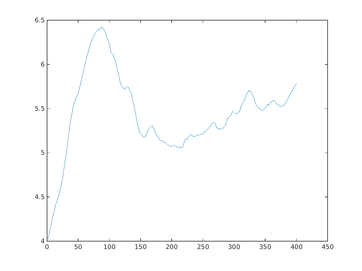
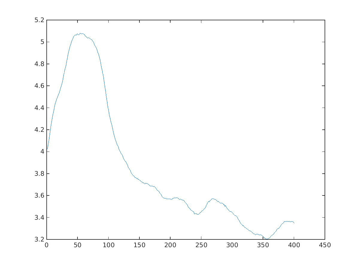
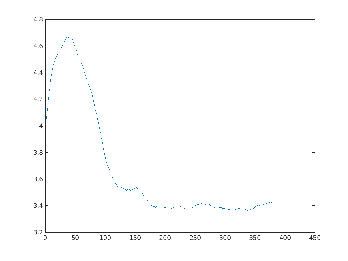
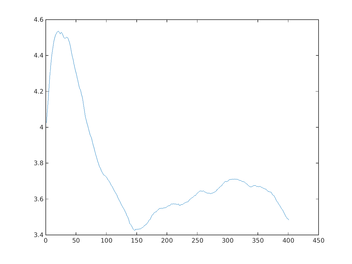
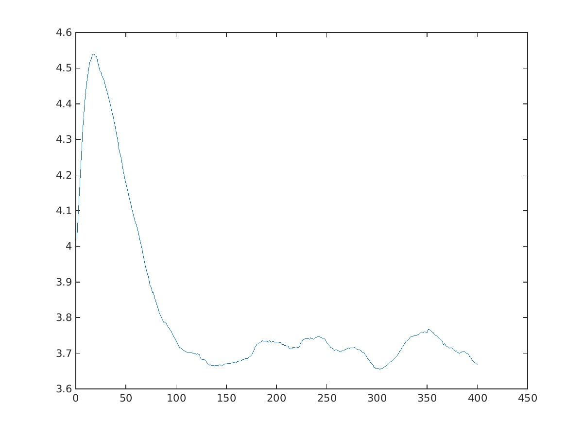
Fig. 6: Values $J^{n_{k},N}_{\alpha}(n_{k+1})$ for different regularization parameters $\alpha_{i}$ plotted against iteration index $k$. Top left: $\alpha_{1}=0.3$, top right: $\alpha_{2}=0.9$, middle left: $\alpha_{3}=1.5$, middle right: $\alpha_{4}=2.1$, bottom: $\alpha_{5}=2.7$.

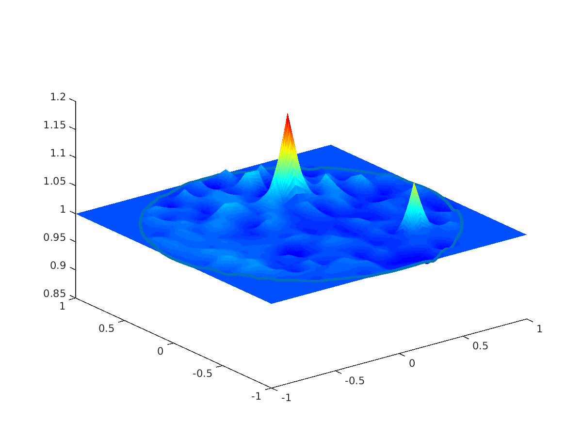
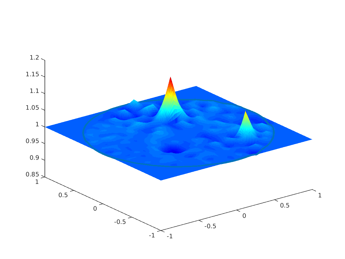
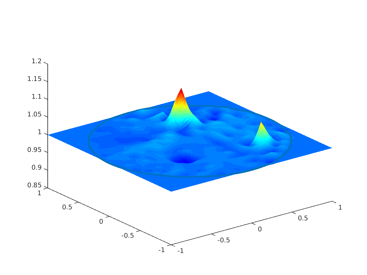
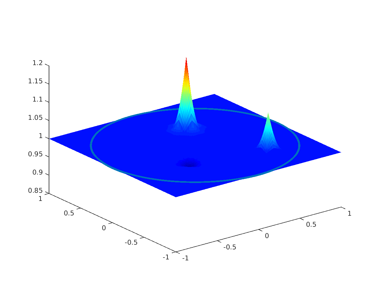
Fig. 7: Exact sound speed $c(x)$ and reconstructions $c_{k^{*}_{i}}(x)$ for different regularization parameters $\alpha_{i}$. Top left: $\alpha_{1}=0.3$, top right: $\alpha_{2}=0.9$, middle left: $\alpha_{3}=1.5$, middle right: $\alpha_{4}=2.1$, bottom left: $\alpha_{5}=2.7$, bottom right: original sound speed.

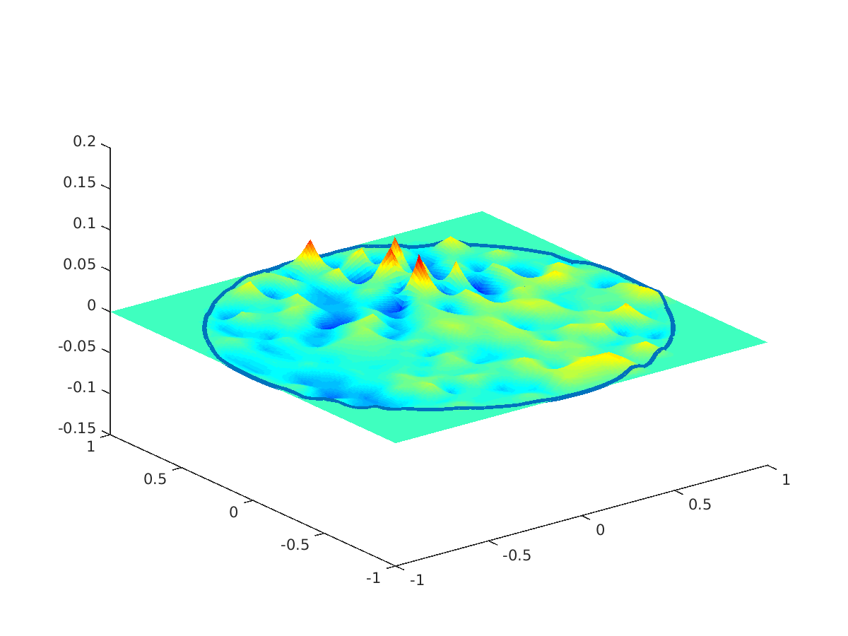
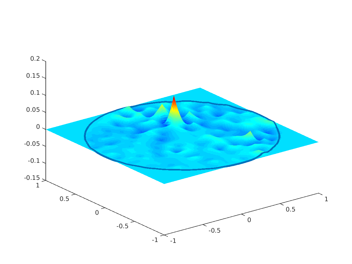
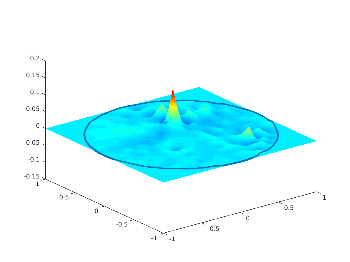
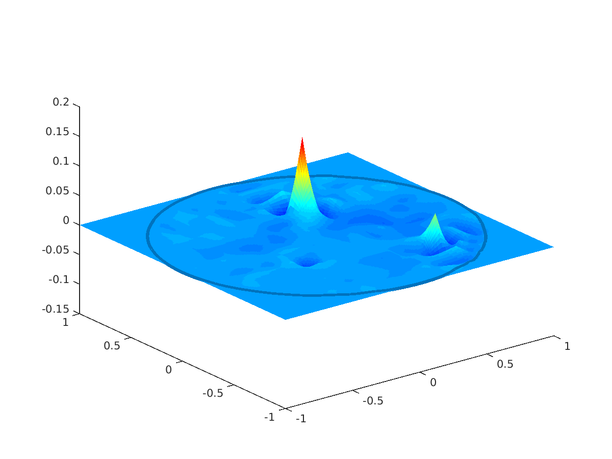
Fig. 8: Errors $c(x)-c_{k^{*}_{i}}(x)$ for different regularization parameters $\alpha_{i}$. Top left: $\alpha_{1}=0.3$, top right: $\alpha_{2}=0.9$, middle left: $\alpha_{3}=1.5$, middle right: $\alpha_{4}=2.1$, bottom: $\alpha_{5}=2.7$.

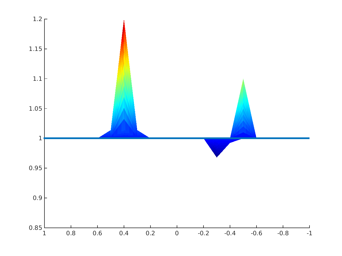
Fig. 9: Exact sound speed $c(x)$ and reconstructions $c_{k^{*}_{i}}(x)$ for different regularization parameters $\alpha_{i}$. Left: original, middle: $\alpha_{1}=0.3$ right: $\alpha_{5}=2.7$.

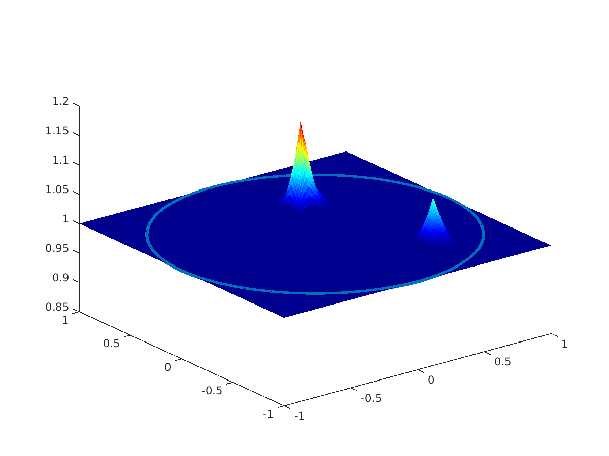
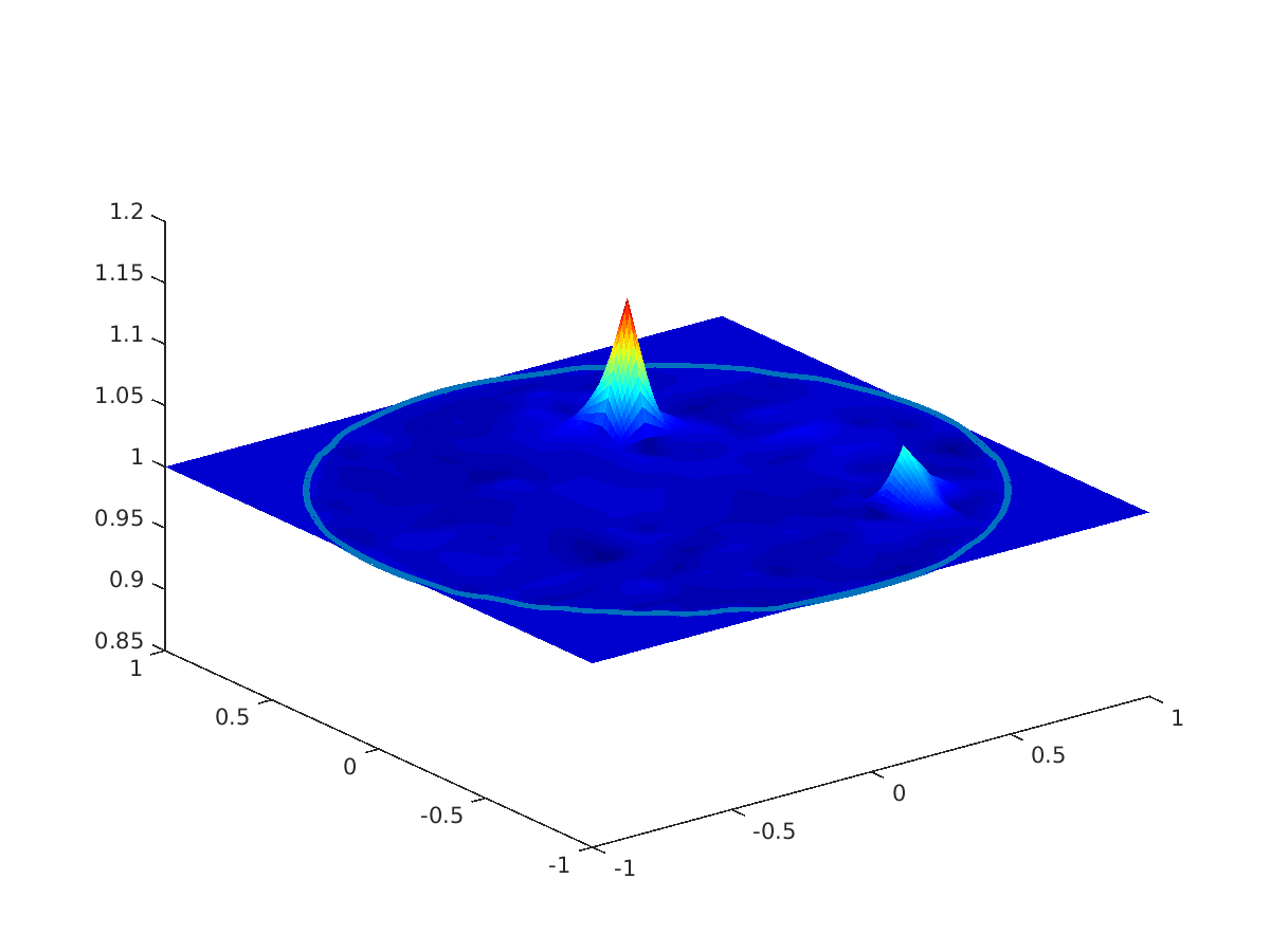
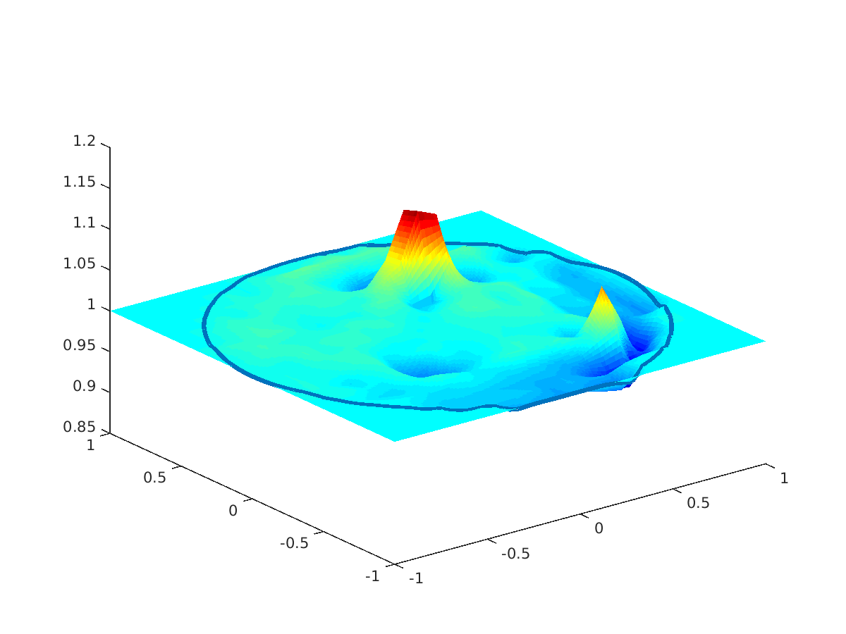
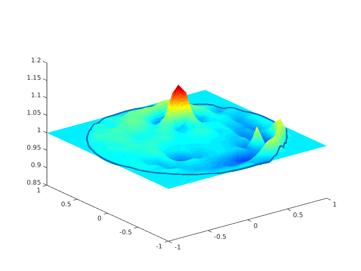
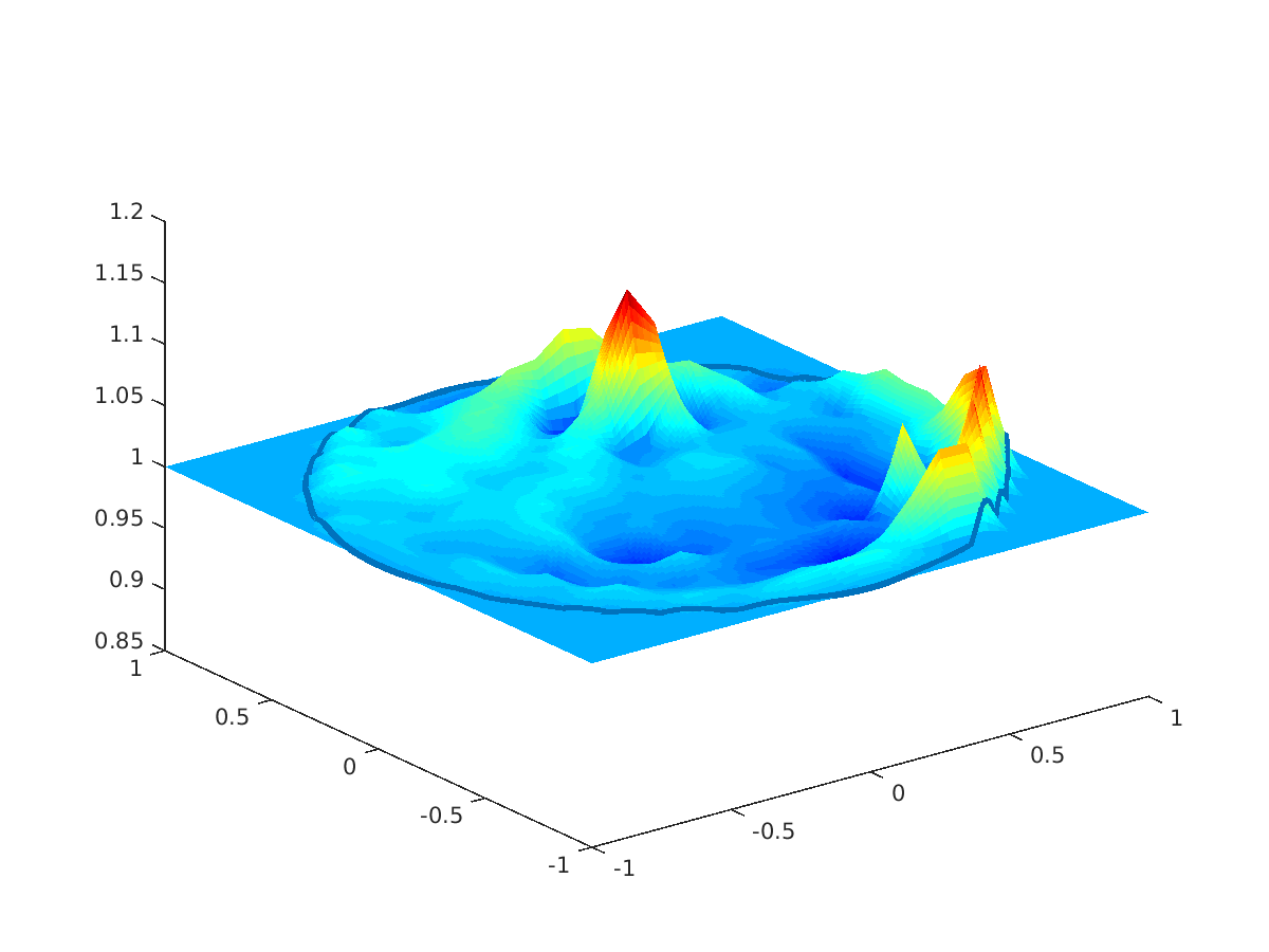
Fig. 10: Reconstructions $c_{k^{*}_{i}}$ for different $p_{i}$-norms. Top left: $p_{1}=1$, top right: $p_{2}=1.1$, middle left: $p_{3}=2$, middle right: $p_{4}=4$, bottom left: $p_{5}=10$, bottom right: exact sound speed.

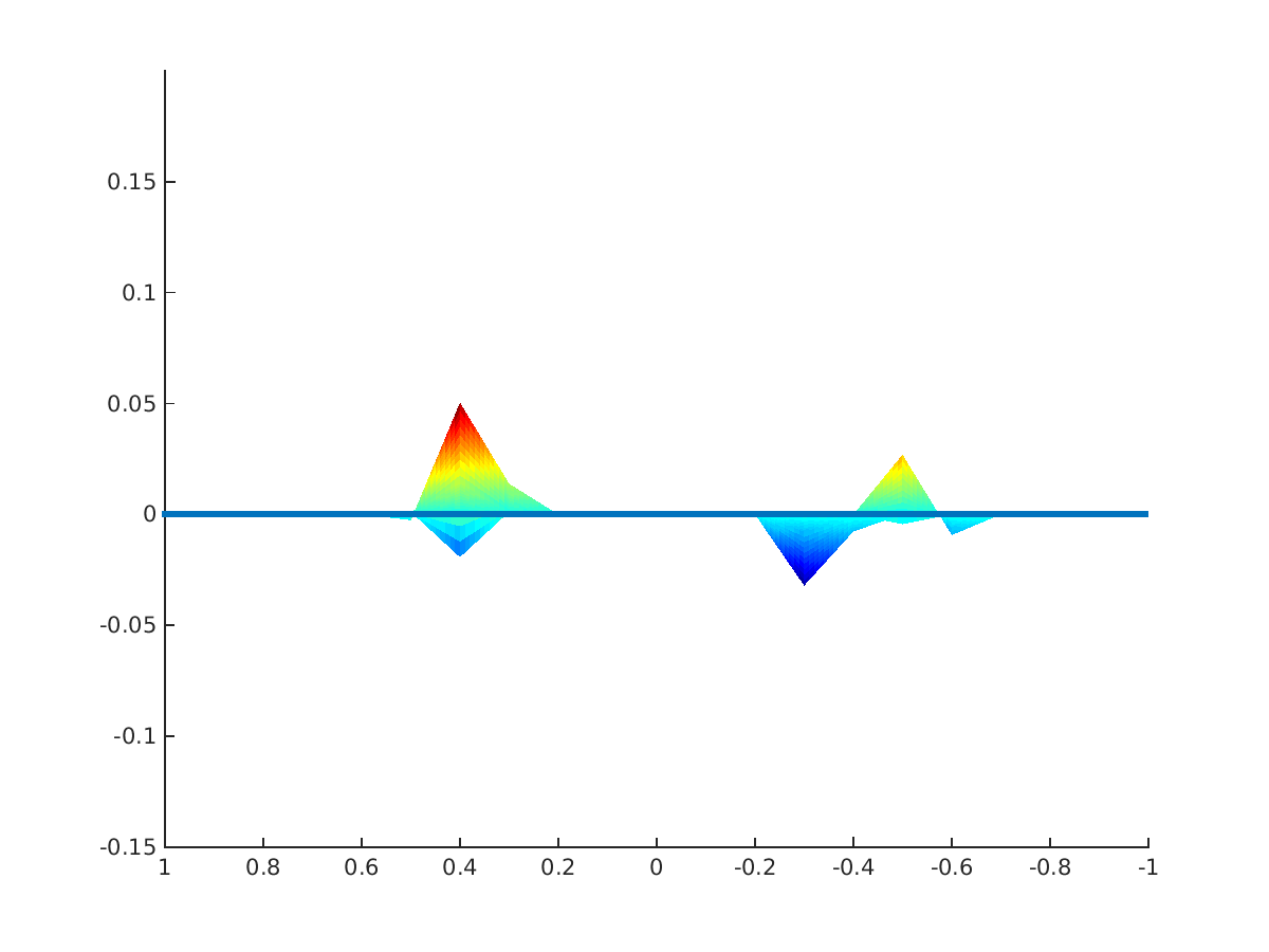
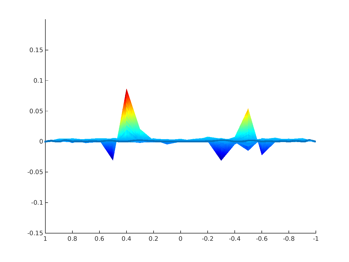
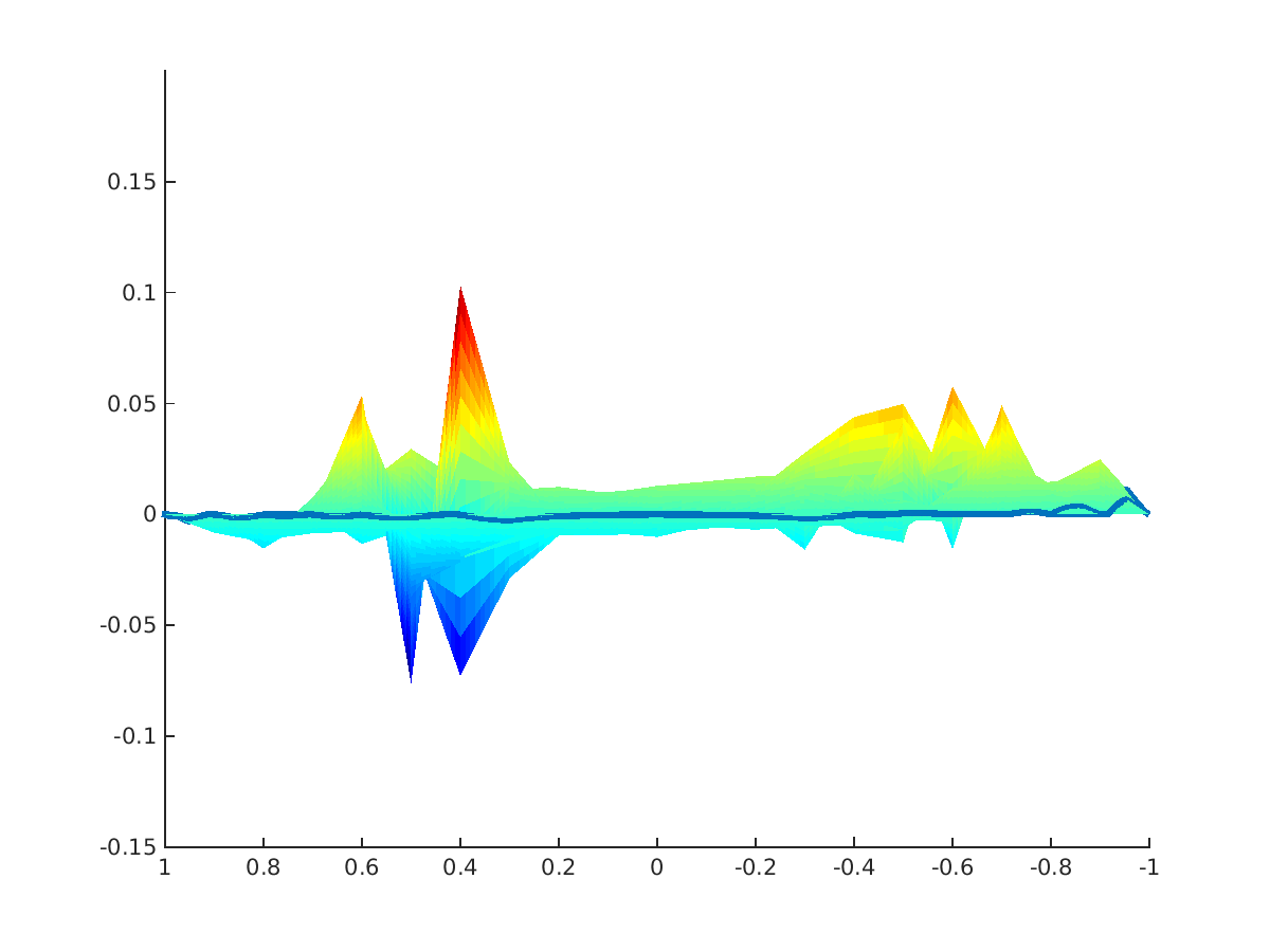
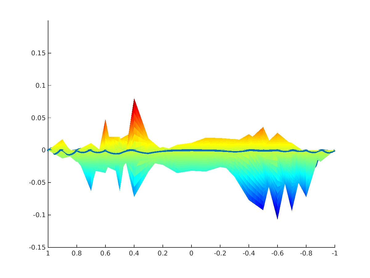
Fig. 11: Errors $c(x)-c_{k^{*}_{i}}(x)$. Top left: $p_{1}=1$, top right: $p_{2}=1.1$, middle left: $p_{3}=2$, middle right: $p_{4}=4$, bottom: $p_{5}=10$.

4.1.2 Different p normes

Again we consider the exact speed of sound (21) but now we calculate reconstructions with different $p$-norms. More explicitly we set

$$p_{1}=1,\,p_{2}=1.1,\,p_{3}=2,\,p_{4}=4\text{ and }p_{5}=10.$$

In case $p_{1}=1$ we implemented the soft threshold method as presented in [8] with $\alpha=0.01$ in this case. For all other $p_{i}$ we set $\alpha=0.2$. In this series of reconstructions we chose $N_{x}=80$ and $N_{\xi}=80$ yielding $\left|\overline{\Gamma}_{N}^{h}\right|=6400$ geodesics to be computed in each iteration setp. The computation of a full set of geodesics lasts about $70$ seconds, the evaluation of $R_{n_{k}}^{*}$ about 20 seconds. In every iteration step we make one descent step with step size parameter $\mu^{1}=0.05$. The uinit square was discretized again using $h=0.1$. The optimal stopping indices $k^{*}_{i}$, $i=1,\ldots,5$ were

$$k^{*}_{1}=42,\,k^{*}_{2}=50,\,k^{*}_{3}=8,\,k^{*}_{8}=10\text{ und }k^{*}_{5}=11.$$

The reconstructions are visualized in Figure 10 compared with the exact $c$. As expected the $p_{1}=1$ and $p_{2}=1.1$ norms lead to the best reconstructions because $c(x)$ and thus $n(x)$ is sparse. Particularily the most part of the reconstruction is identical to $1$. For the choices $p_{3}=2$, $p_{4}=4$ and $p_{5}=10$ one discovers increasing smoothness but also fluctuations of the solution. It is interesting that the small peak at $q_{3}=(0.5,-0.5)$ seems to cause severe artifacts at the boundary $\partial\mathbb{B}$ for $p_{5}=10$. This is also emphasized in Figure 11 where the errors $c(x)-c_{k^{*}_{i}}(x)$ are plotted. Indeed all peaks are detected correctly (the maximal error is about $0.1$), but for higher norms the fluctuations in the Euclidean areas, i.e. areas where $n=1$, increase significantly. Particularily the error is as large as the detected peaks. The artifacts close to the boundary $\partial\mathbb{B}$ become also obvious when comparing the traces of the geodesics obtained for $p_{1}=1$ and $p_{5}=10$ to those of the exact solution $n(x)$, see Figure 12. The left picture shows a good match of the reconstructed and approximated set of geodesics $\mathcal{G}_{k^{*}}$, whereas one clearly recognizes big aberrations in the picture to the right.

Fig. 12: Traces of reconstructed geodesics. The black curves are geodesics of the exact refractive index $n(x)$, the red curves are geodesics of the reconstructions $n_{k^{*}}$. Left picture: $p_{1}=1$, $k^{*}=42$, Right picture: $p_{5}=10$, $k^{*}=11$.

4.2 Sound speed with ’constant curvature’

Next we consider a sound speed which is not sparse. Let

$$c(x)=1/n(x):=1+\varphi(x)\chi_{\mathbb{B}}(x)$$

with

$$\varphi(x)=\frac{(R^{2}+d^{2}|x|^{2})^{2}}{4R^{2}}$$

and the parameters $d=1.2$, $R=2$. The Riemannian manifold $(\mathbb{B},g^{n})$ has then constant, positive Gaussian curvature $K=d^{2}$. Reconstructions for $p$-norms with $p_{1}=1$, $p_{2}=2$ can be seen in Figure 13. The regularization parameters were $\alpha_{1}=0.01$ and $\alpha_{2}=0.4$, respectively. The stopping indices were $k^{*}_{1}=50$ and $k^{*}_{2}=20$, respectively. As expected the reconstruction for $p_{2}$ is more accurate then the sparse reconstruction for $p_{1}$. We furthermore realize that at the center the reconstruction deteriorates. This comes from the specific metric $g^{n}$ which generates a cold spot in the center, that means a small region where almost no geodesic curve, i.e. ultrasound signal, intersects. This fact is clearly visible when we consider the associated geodesic curves for $n$ and $n_{k^{*}_{2}}$ (Figure 14). One sees that only few geodesics pass the center of the disk.

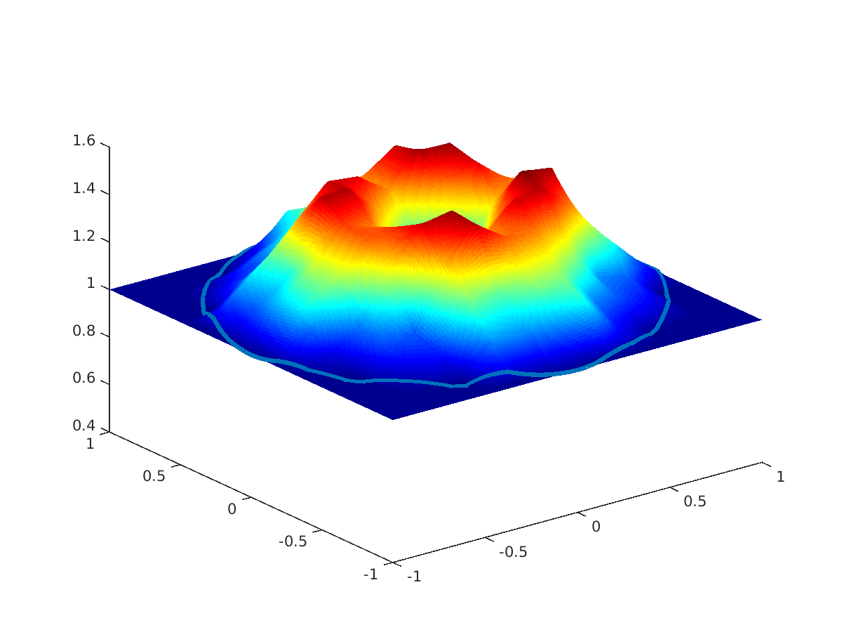
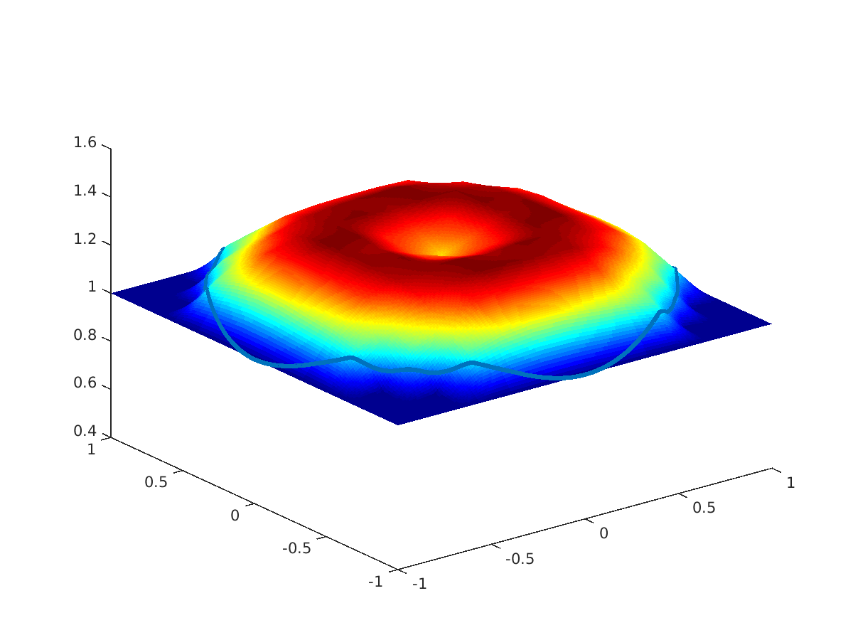
Fig. 13: Reconstructions of a refrective index with constant, positive curvature. Left: $p_{1}=1$, Middle: $p_{2}=2$, Right: exact sound speed.

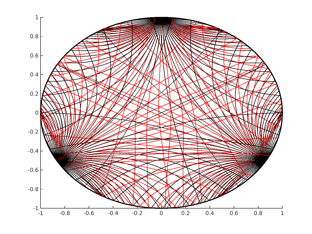
Fig. 14: Geodesic curves for $n_{k^{*}_{2}}$ (red curves) and $n$ (black curves). The cold spot in the center is clearly visible.

4.3 Experiments with noisy data

At last we show a numerical test using noise contaminated data $u^{meas,\delta}$. We perform this test by means of the exact solution

$$c(x)=1/n(x):=1+\sum_{i=1}^{3}\varphi_{i}(x)\chi_{i}(x)+\bar{\varphi}(x)\bar{\chi}(x)$$

with $\varphi_{i}$, $\chi_{i}$ as in Subsection 4.1 and

$$\bar{\varphi}(x)=\bar{\vartheta}\cos\left(\pi\frac{|x-\bar{q}|}{\bar{r}}\right)\,,$$

$$\bar{\chi}(x)=\left\{\begin{array}[]{r@{\,,\quad}l}1&\mbox{if }1-4\bar{r}\leq|x-\bar{q}|\leq 1-2\bar{r}\\ 0&\mbox{else}\,,\end{array}\right.$$

and the parameters $\bar{r}=0.1$, $\bar{q}=(0,0)$. The measure data additionally have been contaminated by unifromly distributed noise $\delta$,

$$u^{meas,\delta}:=R(n^{h})+\delta$$

with relative error $|\delta|/|R(n^{h})|=0.1$ (i.e. $10\%$ relative noise). Figure 15 shows reconstructions with exact $u^{meas}=R(n)$ as well as with noisy data $u^{meas,\delta}$. The parameters for the reconstruction with noisy data are $\mu_{l}=0.02$, $\alpha=1.5$, $p=2$ and $k^{*}=50$.

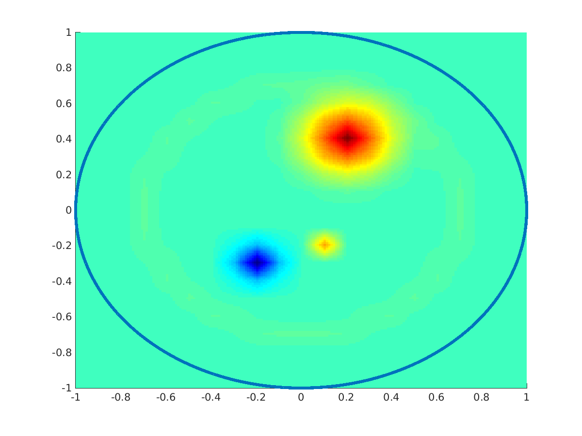
Fig. 15: Reconstructions of $c(x)$ (left picture) from exact data $u^{meas}$ (middle picture) and noisy data $u^{meas,\delta}$ (right picture).

5 Conclusions

In the article we propose a numerical solution scheme for the computation of the refrecative index of a medium from boundary time-of-flight measurements in 2D. The method relies on the minimization of a Tikhonov functional that penalizes aberrations from $n=1$. The minimization is done by a steepest descent method where the linearization of the forward operator was achieved by using the old iteration $n_{k}$ as refractive index to compute the propagation paths. The ultrasound signals were assumed to propagate along geodesics of the Riemannian metric $\mathrm{d}s^{2}=n^{2}(x)|\mathrm{d}x|^{2}$ which is due to Fermat’s principle. We were able to prove that every sequence $\{n_{k}\}$ generated by our iterative scheme has weak limit points. Of course this is a little unsatisfactory. It would be great if one could prove that these limit points are minimizers of $J_{\alpha}$. One way to do this might be to use the concept of surrogate functionals, see e.g. [28, 15]. In fact if we define $\tilde{J}_{\alpha}:X_{p}\times X_{p}\to\mathbb{R}$ by

$$\tilde{J}_{\alpha}(x,a):=J_{\alpha}^{a}(x)\,,$$

then obviously our Algorithm 24 reads as

$$n_{k+1}=\mathrm{arg}\,\min_{n\in L^{p}(M)}\tilde{J}_{\alpha}(n,n_{k})\,,\qquad k=0,1,\ldots.$$

If we assume that $J_{\alpha}(n)\leq\tilde{J}_{\alpha}(n,a)$ at least for all $a$ close to $n$, then $\tilde{J}_{\alpha}$ can be interpreted as a (local) surrogate functional. The investigation of convcergence as well as the derivation of the Gâteaux derivative $R^{\prime}(n)a$, $n,a\in X_{p}$ is subject of current research.
The numerical experiments show a good performance of the method, also if we have sparse solutions.
Another result of the article is the explicit representation of the backprojection operator $R_{a}^{*}$ for a non-Euclidean geometry as well as its numerical realization. We showed the analogy to the conventional (Euclidean) backprojection operator as it is known from 2D computerized tomography.
At last we would like to mention that the results of this article do not only affect seismics or phase contrast TOF tomography, but also other tomographic problems in inhomogeneous media such as vector and tensor field tomography.

References

- [1] M. Agranovsky and P. Kuchment, Uniqueness of reconstruction and an inversion procedure for thermoacoustic and photoacoustic tomography with variable sound speed, Inverse Problems, 23(5) (2007), pp. 2089–2102.
- [2] G. Beylkin, The inversion and application of the generalized Radon transform, Commun. Pure Appl. Math., 37 (1984), pp. 579–599.
- [3] E. Chung, J. Qian, G. Uhlmann, and H. Zhao, A new phase space method for recovering index of refraction from travel times, Inverse Problems, 23 (2007), pp. 309–329.
- [4] C.B. Croke, Rigidity for surfaces of non-positive curvature, Commentarii Mathematici Helvetici, 65 (1990), pp. 150–169.
- [5] , Rigidity and the distance between boundary points, J. Diff. Geom., 33 (1991), pp. 445–464.
- [6] , Rigidity theorems in Riemannian geometry, in Geometric Methods in Inverse Problems and PDE Control, Springer, 2004, pp. 47–72.
- [7] C.B. Croke, N. Dairbekov, and V.A. Sharafutdinov, Local boundary rigidity of a compact Riemannian manifold with curvature bounded above, Transactions of the American Mathematical Soc., 9 (2000), pp. 3937–3956.
- [8] I. Daubechies, M. Defrise, and C. De Mol, An iterative thresholding algorithm for linear inverse problems with a sparsity constraint, Communications on Pure and Applied Mathematics, 11 (2004), pp. 1413–1457.
- [9] E.Y. Derevtsov, R. Dietz, A.K. Louis, and T. Schuster, Influence of refraction to the accuracy of a solution for the 2D-emission tomography problem, J. Inv. Ill-Posed Problems, 8(2) (2000), pp. 161–191.
- [10] V. Guillemin and S. Sternberg, Geometric asymptotics, American Mathematical Soc., 14 (1990).
- [11] M. Gromov, Filling Riemannian manifolds, Journal of Differential Geometry, 18 (1983), pp. 1–147.
- [12] G. Herglotz, Über die Elastizität der Erde bei Berücksichtigung ihrer variablen Dichte (On the elasticity of the earth taking a variable density into account), Zeitschr. für Math. Phys, 52 (1905), pp. 275–299.
- [13] B. Hofmann, B. Kaltenbacher, C. Poeschl, and O. Scherzer, A convergence rates result for Tikhonov regularization in Banach spaces with non-smooth operators, Inverse Problems, 23 (2007).
- [14] M.V. Klibanov and V.G. Romanov, Reconstruction procedures for two inverse scattering problems without phase information, arXiv:1505.01905v1 (2015).
- [15] K. Lange, D.R. Hunter, and I. Yang, Optimization transfer using surrogate objective functions, Journal of Computational and Graphical Statistics, 9 (2000), pp. 1–20.
- [16] M. Lassas, V.A. Sharafutdinov, and G. Uhlmann, Semiglobal boundary rigidity for Riemannian metrics, Mathematische Annalen, 325 (2003), pp. 767–793.
- [17] S. Lovett, Differential Geometry of Manifolds, CRC Press, 2010.
- [18] R. Michel, Sur la rigidité imposée par la longueur des géodésiques, Inventiones Mathematicae, 65 (1981), pp. 71–83.
- [19] F. Monard, Numerical implementation of geodesic X-ray transforms and their inversion, SIAM J. Imag. Sci., 7(2) (2014), pp. 1335–1357.
- [20] R.G. Mukhometov, Inverse kinematic problem of seismic on the plane, Math. Problems of Geophysics. Akad. Nauk. SSSR, Sibirsk. Otdel., Vychisl. Tsentr, Novosibirsk, 6 (1975), pp. 243–252.
- [21] , A problem of reconstructing a Riemannian metric, Siberian Mathematical Journal, 22 (1981), pp. 420–433.
- [22] F. Natterer, The Mathematics of Computerized Tomography, Wiley, Chichester, 1986.
- [23] S.J. Norton, Tomographic reconstruction of 2-D vector fields: application to flow imaging, Geophysical Journal International, 97 (1988), pp. 161–168.
- [24] J.-P. Otal, Sur les longueurs des géodésiques d’une métrique à courbure négative dans le disque, Commentarii Mathematici Helvetici, 65 (1990), pp. 334–347.
- [25] L. Pestov and G. Uhlmann, Two dimensional compact simple Riemannian manifolds are boundary distance rigid, Annals of mathematics, 161(2) (2005), pp. 1093–1110.
- [26] T. Pfitzenreiter and T. Schuster, Tomographic reconstruction of the curl and divergence of 2D vector fields taking refractions into account, SIAM Journal on Imaging Sciences, 4 (2011), pp. 40–56.
- [27] J. Qian, P. Stefanov, G. Uhlmann, and H. Zhao, An efficient Neumann series-based algorithm for thermoacoustic and photoacoustic tomography with variable sound speed, SIAM J. Imag. Sci., 4(3) (2011), pp. 850–883.
- [28] R. Ramlau and G. Teschke, A Tikhonov-based projection iteration for nonlinear Ill-posed problems with sparsity constraints, Numerische Mathematik, 104(29 (2006), pp. 177–203.
- [29] V.G. Romanov, Integral geometry on geodesics of isotropic Riemannian metric, Doklady Akademii Nauk SSSR, 241 (1978), pp. 290–293.
- [30] F. Schöpfer, A.K. Louis, and T. Schuster, Nonlinear iterative methods for linear ill-posed problems in Banach spaces, Inverse Problems, 22(1) (2006), pp. 311–329.
- [31] T. Schuster, B. Kaltenbacher, B. Hofmann, and K. Kazimierski, Regularization Methods in Banach spaces, de Gruyter, 2012.
- [32] V.A. Sharafutdinov, Integral Geometry of Tensor Fields, VSP, Utrecht, 1994.
- [33] , Ray transform on Riemannian manifolds, in New analytic and geometric methods in inverse problems, Springer, 2004, pp. 187–259.
- [34] P. Stefanov and G. Uhlmann, Rigidity for metrics with the same lengths of geodesics, Mathematical Research Letters, 5 (1998), pp. 83–96.
- [35] , Stability estimates for the X-ray transform of tensor fields and boundary rigidity, Duke Math. J., 123(3) (2004), pp. 445-467.
- [36] , Local lens rigidity with incomplete data for a class of non-simple Riemannian manifolds, J. Differential Geom., 82(2) (2009), pp. 383-409.
- [37] P. Stefanov, G. Uhlmann, and A. Vasy, Inverting the local geodesic X-ray transform on tensors, arXiv:1410.5145 (2014).
- [38] I.E. Svetov, E.Y. Derevtsov, Y.S. Volkov, and T. Schuster, A numerical solver based on B-splines for 2D vector field tomography in a refracting medium, Mathematics and Computers in Simulation, 97 (2014), pp. 207–223.
- [39] W. Walter, Ordinary Differential Equations, Springer, Berlin, 1998.