The ${\mathcal{N}}=2$ Schur index from free fermions

Abstract:

We study the Schur index of 4-dimensional ${\mathcal{N}}=2$ circular quiver theories. We show that the index can be expressed as a weighted sum over partition functions describing systems of free Fermions living on a circle. For circular $SU(N)$ quivers of arbitrary length we evaluate the large $N$ limit of the index, up to exponentially suppressed corrections. For the single node theory (${\mathcal{N}}=4$ SYM) and the two node quiver we are able to go beyond the large $N$ limit, and obtain the complete, all orders large $N$ expansion of the index, as well as explicit finite $N$ results in terms of elliptic functions.

1 Introduction and Results

Supersymmetric field theories have seen dramatic advances in recent years, many brought about through the study of partition functions on compact manifolds admitting Killing spinors. Most often those are the sphere partition function and the superconformal index related to the $S^{d-1}\times S^{1}$ partition function. The latter, first introduced for 4-dimensional theories in [1, 2], is a generalization of the Witten index [3]. As such, it counts the states of the theory according to their fermionic or bosonic nature, as well as according to their quantum numbers. These charges, for symmetries which commute with the Hamiltonian and preserved supercharges, are introduced in the usual trace formula through fugacities.

In this paper we study the index of $4d$ $\mathcal{N}=2$ superconformal theories on $S^{3}\times S^{1}$. The representations of the corresponding superconformal algebra $SU(2,2|2)$ are labelled by the Cartans $(E,j_{1},j_{2},R,r)$ of its bosonic subalgebra. $E$ is the energy, $(j_{1},j_{2})$ are the Cartans of the $SU(2)_{1}\otimes SU(2)_{2}$ isometries and $(R,r)$ are the Cartans of the $SU(2)_{R}\otimes U(1)_{r}$ $R$-symmetry group.

The superconformal index generally has three independent fugacities coupling to linear combinations of these Cartans, and in addition fugacities for flavour symmetries (see Appendix A). We are interested in an unrefined version of the index, known as the Schur index [4, 5, 6], where one relation is imposed between the three fugacities, but it turns out that the resulting index depends only on one unique fugacity $q$. The charge that this fugacity couples to commutes with a pair of supercharges $Q$ and $Q^{\prime}$, which, following [5, 7], we choose such that

$$\delta \equiv 2\{Q,Q^{\dagger}\}=E-2j_{2}-2R+r\,,$$ (1)

$$\delta^{\prime} \equiv 2\{Q^{\prime},{Q^{\prime}}^{\dagger}\}=E+2j_{1}-2R-r\,.$$

The Schur index is then given by

$$\mathcal{I}=\operatorname{Tr}(-1)^{F}e^{\beta\delta}e^{\beta^{\prime}\delta^{\prime}}q^{2\left(E-R\right)}\prod_{a}e^{2iu^{(a)}F^{(a)}}\,,$$ (2)

where $q$ and $e^{2iu^{(a)}}$ are the fugacities for the charges of the superconformal and flavour groups respectively, and $F^{(a)}$ are the flavour charges. We express the flavour fugacities in terms of their chemical potentials $u^{(a)}$, which appear in a natural way in the explicit expressions for the index below. The sum in (2) is taken over all states of the theory, but following the usual Witten argument [3], contributions from fermions and bosons cancel for all multiplets except for those with $\delta=\delta^{\prime}=0$, so that the index is independent of $\beta,\beta^{\prime}$.

As shown in [1, 2], there is an elegant way to express the index (2) as a matrix model. It was first noted in [8] that the contributions from each multiplet can be neatly expressed in terms of elliptic gamma functions. For the Schur index, the contributions combine in such a way that they can be written as $q$-theta functions (see Appendix A and [6]). We give here the expressions for each multiplet, in terms of Jacobi theta functions and the Dedekind eta function (see Appendix B for their definition and for useful identities). We consider $SU(N)$ gauge groups, and use the gauge freedom to reduce the integral over the Lie algebra to an integral over a Cartan subalgebra that we parametrize with $\alpha_{i}$, $i=1,\cdots,N$, which are $\pi$ periodic and which satisfy the traceless condition $\sum_{i=1}^{N}\alpha_{i}=0$ imposed through a delta function.

The contribution from an $\mathcal{N}=2$ vector multiplet, including the integration with the Haar measure is (121)

$$\mathcal{I}_{\text{vec}}=\big{(}q^{-\frac{1}{12}}\eta(\tau)\big{)}^{2(N-1)}\frac{1}{\pi^{N}N!}\int_{0}^{\pi}d^{N}\alpha\delta\left(\sum_{i=1}^{N}\alpha_{i}\right)\prod_{i<j}\frac{\vartheta_{1}^{2}\big{(}\alpha_{i}-\alpha_{j},q\big{)}}{q^{\frac{1}{3}}\eta^{2}(\tau)}\,,$$ (3)

where we have used the notation $q\equiv e^{i\pi\tau}$.

An $\mathcal{N}=2$ hypermultiplet in the bi-fundamental representation of the gauge groups $G^{(1)}\times G^{(2)}$ contributes to the index as (118)

$$\mathcal{I}_{\text{hyp}}=\prod_{i,j}\frac{q^{-1/12}\eta(\tau)}{\vartheta_{4}\big{(}\alpha^{(1)}_{i}-\alpha^{(2)}_{j}+u,q\big{)}}\,,$$ (4)

where $u$ is the chemical potential for the $U(1)$ flavour symmetry, which enters in the index as defined in (2).

The simplest matrix model of this class corresponds to ${\mathcal{N}}=4$ SYM, which in this ${\mathcal{N}}=2$ formalism has one $U(N)$ gauge group, as well as one adjoint hypermultiplet. The model for this particular case was solved exactly in [9]. This was made possible by expressing the matrix model as the partition function of a 1-dimensional free Fermi gas. In the context of supersymmetric field theories, this type of manipulation was pioneered in [10], who studied the $S^{3}$ partition function of ABJM theory [11], as well as more general circular quiver gauge theories. This led to numerous results, such as the discovery of the universal Airy function behaviour of the perturbative part in the large $N$ expansion for all circular quivers [10], as well as a complete understanding of the non-perturbative effects of the ABJ(M) partition function (see [12] for a review). This formalism was also successfully applied to many other three dimensional superconformal theories, with wide ranging gauge groups [13] and quiver structures [14, 15], and was also used to understand the relationship between topological strings and 3d partition functions [16, 17, 18].

The key step in this method is the use of a determinant identity which expresses the integrand of the matrix model as a determinant. Indeed, in [9] we used an elliptic generalization (140) of the Cauchy determinant identity which resolved the interactions in the matrix model of the index of ${\mathcal{N}}=4$ SYM.

In the present paper we study theories that are a natural generalisation of ${\mathcal{N}}=4$ SYM, namely circular quivers, and apply the Fermi gas formalism to compute the Schur index. A circular quiver of length $L$ has gauge group $SU(N)^{L}$, with vector multiplets for each gauge group factor and bi-fundamental hypermultiplets connecting them in circular fashion, as depicted in figure 1. These theories are of particular interest as the circular structure is most susceptible to a Fermi-gas interpretation in terms of traces of single particle density operators (theories with a quiver structure of a $\hat{D}$ Dynkin diagram are also interesting candidates, and a discussion of these will appear in [19]). It would be interesting to understand whether any of the techniques developed here could also be applied to non-Lagrangian “class-${\mathcal{S}}$” theories.

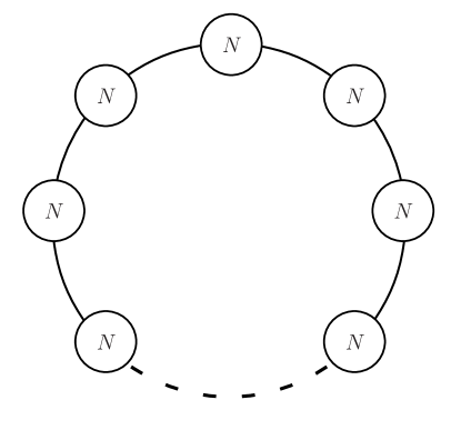
Figure 1: A diagram of ${\mathcal{N}}=2$ circular quiver theories. Each node of the diagram represents a $U(N)$ $SU(N)$ vector multiplet, while a solid lines connecting two nodes represents a bi-fundamental hypermultiplet.

Unlike 3d circular quivers, where many theories with ${\mathcal{N}}\geq 2$ flow to conformal fixed points, in 4d we cannot add extra fundamental hypermultiplets. The resulting theories are neither conformal nor asymptotically free. Nonetheless, it is rather easy to add to the matrix models factors associated to fundamental matter, but since we do not have a 4d interpretation of this, we do not consider these here. Note however that in the calculation of the Schur index of ${\mathcal{N}}=4$ SYM in the presence of Wilson loop operators [20], the matrix model gets enriched by terms somewhat similar to those due to fundamental matter fields. It would be interesting to try to generalize that calculation to the circular quivers studied here and explore this generalization of the matrix model.

We find that for $SU(N)$ circular quivers one can use the elliptic determinant identity to write the index as the partition function describing a set of $N$ interacting fermions. The interaction terms are due to the tracelessness condition,which we avoid handling directly by expanding them in Fourier series, at the cost of introducing an infinite number of terms, each of which can be interpreted as the partition function of a free Fermi gas.

The resulting infinite sum has a natural interpretation as a Fourier expansion in flavour fugacities of a rescaled index (provided the product of the flavour fugacities is $1$). Thus each Fourier coefficient of the rescaled index is given by the aforementioned partition function of a free Fermi gas (14). Each Fermi gas can then be studied independently, and we do so by considering the associated grand canonical partition function with chemical potential $\mu$.

For a circular quiver of arbitrary length we are able to write down (when the product of the flavour fugacities is $1$) a closed formula for the grand partition function (30), involving a product of Jacobi elliptic theta functions evaluated at the roots of a polynomial (33), whose degree grows with the length of the quiver.

In Section 3 we then present a computation which gives the full perturbative (in $N$) expression for the index in the large $N$ limit. We first calculate the leading term of the grand canonical partition function at large chemical potential $\mu$, for which we give two different methods. In one method we solve for the roots of the polynomial (33) in the large $\mu$ limit, while in the other we use a Mellin-Barnes representation of the grand potential to extract its large $\mu$ behaviour. We can then carry out the resummation over the Fourier modes to obtain

$$\mathcal{I}(N,L)=\frac{q^{\frac{L}{6}}}{\eta^{L}(\tau)\eta^{2}(\tfrac{L\tau}{2})}+{\mathcal{O}}(e^{-cN})\,,\qquad c>0\,.$$ (5)

We find here that the leading term is $N$-independent, as was already pointed out in [2] for $\mathcal{N}=4$ SYM, that there are no perturbative $1/N$ corrections, and that the result is also independent of the flavour fugacities.

It should be noted that this scaling does not match the supergravity action, which grows as $N^{2}$. Indeed the correct quantity to compare on the field theory side to the classical supergravity action is the partition function on $S^{3}\times S^{1}$, which is related to our index through a factor, dubbed the supersymmetric Casimir energy [21, 22], which does scale like $N^{2}$. There is still a discrepancy with the supergravity calculation, possibly due to missing counterterms of supersymmetric holographic renormalization. As we see above, we find the same $N^{0}$ scaling for the index of ${\mathcal{N}}=2$ theories, and have not calculated the Casimir energy. It is unclear whether the ${\mathcal{N}}=2$ generalization could shed light on this issue.

In the cases where we can find the non-perturbative corrections at large $N$, which are ${\mathcal{N}}=4$ SYM [9] and the two node quiver (see Section 4), there should be an interpretation of the instanton corrections in terms of some other supergravity saddle points and/or D-brane configurations, but such an understanding is also lacking.

As just mentioned, for short quivers we are able to go beyond the perturbative large $N$ result (5). This is based on the expression for the grand partition function in terms of the roots of a polynomial, which for $L=1$ and $L=2$ is quadratic, so the roots can be obtained explicitly. This allows us to compute the complete, all orders large $N$ expansions of the index for these theories in Section 4. For the two-node case, we find that the independence of the asymptotic expression (5) on the flavour fugacity gets lifted by non-perturbative corrections. Furthermore, in the absence of flavour fugacities, we extract exact results in terms of elliptic integrals for finite values of $N$ in Section 5. Finally in Section 5.3 we are able to obtain similar finite $N$ results also for longer quivers by comparing the $q$ expansion of the index and polynomials of elliptic integrals, and present results for quivers of up to four nodes.

2 Circular quivers as free Fermi gases

Using the formulae given in the introduction, the matrix model for the Schur index of a $SU(N)$ circular quiver gauge theory with $L$ nodes is

$$\mathcal{I}(N,L) =\frac{q^{-\frac{LN^{2}}{4}}q^{\frac{L}{6}}\eta(\tau)^{(3N-2)L}}{N!^{L}\pi^{NL}}\int_{0}^{\pi}\prod_{a=1}^{L}d^{N}\alpha^{(a)}\delta\left(NA^{(L)}\right)\prod_{a=1}^{L-1}\delta\big{(}N\big{(}A^{(a)}-A^{(a+1)}\big{)}\big{)}$$ (6)

$$\hskip 144.54pt\times\frac{\prod_{i<j}\vartheta_{1}\big{(}\alpha^{(a)}_{i}-\alpha^{(a)}_{j}\big{)}\vartheta_{1}\big{(}\alpha^{(a+1)}_{i}-\alpha^{(a+1)}_{j}\big{)}}{\prod_{i,j}\vartheta_{4}\big{(}\alpha^{(a)}_{i}-\alpha^{(a+1)}_{j}+u^{(a)}\big{)}}\,,$$

where it is understood that $\alpha^{(L+1)}_{i}=\alpha^{(1)}_{i}$, and we have used the notation $\vartheta_{i}(z)=\vartheta_{i}(z,q)$, and introduced the centers of mass

$$A^{(a)}=\frac{1}{N}\sum_{i=1}^{N}\alpha_{i}^{(a)}\,.$$ (7)

We allow here for arbitrary chemical potentials $u^{(a)}$ for the flavour symmetries of the hypermultiplets. The $L$ delta function constraints in (6) come from the tracelessness condition, and we have chosen to represent all but one of them in difference form. Note that for the single node theory ($\mathcal{N}=4$ SYM) the traceless condition also applies to the hypermultiplet, where the adjoint is of dimension $N^{2}-1$ rather than $N^{2}$. This introduces and additional factor of $q^{\frac{1}{12}}\eta^{-1}(\tau)\vartheta_{4}(u)$.

The second line in (6) can be rewritten using an elliptic determinant identity (140) given in Appendix C

$$\frac{\prod_{i<j}\vartheta_{1}\big{(}\alpha^{(a)}_{i}-\alpha^{(a)}_{j}\big{)}\vartheta_{1}\big{(}\alpha^{(a+1)}_{i}-\alpha^{(a+1)}_{j}\big{)}}{\prod_{i,j}\vartheta_{4}\big{(}\alpha^{(a)}_{i}-\alpha^{(a+1)}_{j}+u^{(a)}\big{)}}=\left(\frac{\vartheta_{2}}{\vartheta_{4}\vartheta_{3}}\right)^{N}$$ (8)

$$\hskip 14.22636pt\times\frac{\vartheta_{3}\,q^{-\frac{N^{2}}{4}}e^{iN^{2}(A^{(a)}-A^{(a+1)}+u^{(a)})}}{\vartheta_{3}\big{(}N(A^{(a)}-A^{(a+1)}+u^{(a)}+\tfrac{\pi\tau}{2})\big{)}}\det_{ij}\left(\operatorname{cn}\big{(}\big{(}\alpha_{i}^{(a)}-\alpha_{j}^{(a+1)}+u^{(a)}\big{)}\vartheta_{3}^{2}\big{)}\right)\,,$$

where we have used the notation $\vartheta_{i}=\vartheta_{i}(0,q)$.

Putting this together allows us to write the index as

$$\mathcal{I}(N,L)=\frac{q^{-\frac{N^{2}L}{2}}e^{-iN^{2}U}q^{\frac{L}{6}}}{\eta^{2L}(\tau)}\prod_{a=1}^{L}\frac{\vartheta_{3}}{\vartheta_{3}\big{(}Nu^{(a)}+N\frac{\pi\tau}{2}\big{)}}\,Z(N)$$ (9)

where $U=\sum_{a=1}^{L}u^{(a)}$ and where we have used the identity (129) to simplify the $\alpha$-independent factor. $Z(N)$ is defined as

$$Z(N,L) =\frac{1}{N!^{L}}\int_{0}^{\pi}\prod_{a=1}^{L}d^{N}\alpha^{(a)}\delta\left(NA^{(L)}\right)\prod_{a=1}^{L-1}\delta\left(N\left(A^{(a)}-A^{(a+1)}\right)\right)$$ (10)

$$\quad{}\times\det_{ij}\bigg{(}\frac{\vartheta_{2}^{2}}{2\pi}\operatorname{cn}\big{(}(\alpha_{i}^{(a)}-\alpha_{j}^{(a+1)}+u^{(a)})\vartheta_{3}^{2}\big{)}\bigg{)},$$

Each determinant can then be written as a sum over permutations, and by relabelling the eigenvalues, one can factor all but one of the permutations, picking up a factor of $N!^{L-1}$ and leading to

$$Z (N,L)=\frac{1}{N!}\sum_{\sigma\in S^{N}}(-1)^{\epsilon(\sigma)}\int_{0}^{\pi}\prod_{a=1}^{L}d^{N}\alpha^{(a)}\,\delta\left(NA^{(L)}\right)\prod_{a=1}^{L-1}\delta\big{(}N\big{(}A^{(a)}-A^{(a+1)}\big{)}\big{)}$$ (11)

$$\quad{}\times\prod_{i=1}^{N}\bigg{(}\prod_{a=1}^{L-1}\frac{\vartheta_{2}^{2}}{2\pi}\operatorname{cn}\big{(}(\alpha_{i}^{(a)}-\alpha_{i}^{(a+1)}+u^{(a)})\vartheta_{3}^{2}\big{)}\bigg{)}\frac{\vartheta_{2}^{2}}{2\pi}\operatorname{cn}\big{(}(\alpha_{i}^{(L)}-\alpha_{\sigma(i)}^{(1)}+u^{(L)})\vartheta_{3}^{2}\big{)},$$

This expression strongly suggests that the eigenvalues describe fermionic degrees of freedom. The difficulty in writing down a single particle density operator comes from the presence of the center of mass coordinates $A^{(a)}$ in the delta functions, which introduce complicated interactions.

To overcome it we first shift the eigenvalues as $\alpha^{(a)}\rightarrow\alpha^{(a)}+\sum_{b=1}^{a-1}u^{(b)}$ so that the $u$’s appear only inside the delta functions and one $\operatorname{cn}$

$$Z(N,L) =\sum_{\sigma\in S^{N}}\left(-1\right)^{\epsilon(\sigma)}\int_{0}^{\pi}\prod_{a=1}^{L-1}d^{N}\alpha^{(a)}\delta\big{(}N(A^{(a)}-A^{(a+1)}-u^{(a)})\big{)}$$ (12)

$$\quad{}\times\int_{0}^{\pi}d^{N}\alpha^{(L)}\delta\big{(}N(A^{(L)}+U-u^{(L)})\big{)}$$

$$\quad{}\times\prod_{i=1}^{N}\bigg{(}\frac{\vartheta_{2}^{2}}{2\pi}\operatorname{cn}\big{(}(\alpha_{i}^{(L)}-\alpha_{\sigma(i)}^{(1)}+U)\vartheta_{3}^{2}\big{)}\prod_{a=1}^{L-1}\frac{\vartheta_{2}^{2}}{2\pi}\operatorname{cn}\big{(}(\alpha_{i}^{(a)}-\alpha_{i}^{(a+1)})\vartheta_{3}^{2}\big{)}\bigg{)},$$

Now we represent the delta functions by their Fourier expansion

$$\delta \big{(}N(A^{(L)}+U-u^{(L)})\big{)}\prod_{a=1}^{L-1}\delta\big{(}N(A^{(a)}-A^{(a+1)}-u^{(a)})\big{)}$$ (13)

$$=\sum_{\vec{n}\in\mathbb{Z}^{L}}e^{-2iN\sum_{a=1}^{L}n^{(a)}u^{(a)}}e^{2iNUn^{(L)}}e^{2in^{(L)}\sum_{i}\alpha^{(L)}_{i}}\prod_{a=1}^{L-1}e^{2in^{(a)}\sum_{i}(\alpha^{(a)}_{i}-\alpha^{(a+1)}_{i})}\,,$$

with $\vec{n}=\{n^{(a)}\}$. We can then write the rescaled index as a sum

$$Z(N,L)=\sum_{\vec{n}\in\mathbb{Z}^{L}}e^{-2iN\sum_{a=1}^{L}n^{(a)}u^{(a)}}e^{2iNUn^{(L)}}Z_{\vec{n}}\,.$$ (14)

Now each Fourier coefficient $Z_{\vec{n}}$ is a partition function of a free Fermi gas expressed as

$$Z_{\vec{n}} =\frac{1}{N!}\sum_{\sigma\in S^{N}}(-1)^{\epsilon(\sigma)}\int_{0}^{\pi}d^{N}\alpha_{i}\prod_{i}^{N}\rho_{\vec{n}}(\alpha_{i},\alpha_{\sigma(i)})\,,$$ (15)

in terms of a single particle density operator

$$\rho_{\vec{n}}\big{(}\alpha^{(1)},\alpha^{(L+1)}\big{)}=\int_{0}^{\pi}\prod_{a=2}^{L}d\alpha^{(a)}\,e^{2in^{(L)}\alpha^{(L)}}\frac{\vartheta_{2}^{2}}{2\pi}\prod_{a=1}^{L-1}e^{2in^{(a)}(\alpha^{(a)}-\alpha^{(a+1)})}$$ (16)

$$\hskip 56.9055pt\times\operatorname{cn}\big{(}(\alpha^{(L)}-\alpha^{(L+1)}+U)\vartheta_{3}^{2}\big{)}\prod_{a=1}^{L-1}\frac{\vartheta_{2}^{2}}{2\pi}\operatorname{cn}\big{(}(\alpha^{(a)}-\alpha^{(a+1)})\vartheta_{3}^{2}\big{)}\,,$$

where in $Z_{\vec{n}}$ we substitute $\alpha^{(1)}=\alpha_{i}$ and $\alpha^{(L+1)}\equiv\alpha_{\sigma(i)}$. In fact, this Fourier expansion closely mirrors the original definition of the index with flavour fugacities (2) and were it not for the $u$ dependence in the rescaling factor in (9), then $Z_{\vec{n}}$ would be the index for fixed flavour charges $F^{(a)}=-Nn^{(a)}$.

The Fermi gas partition function (15) is completely determined by

$$Z_{\vec{n};\ell}=\operatorname{Tr}(\rho_{\vec{n}}^{\ell})=\int_{0}^{\pi}dx_{1}\cdots dx_{\ell}\,\rho_{\vec{n}}(x_{1},x_{2})\cdots\rho_{\vec{n}}(x_{\ell},x_{1})\,,$$ (17)

often referred to as the spectral traces. Indeed, conjugacy classes of $S_{N}$ have $m_{\ell}$ cycles of length $\ell$, and from the definition (15) of $Z_{\vec{n}}(N)$ we get

$$Z_{\vec{n}}(N)={\sum_{\{m_{\ell}\}}}^{\prime}\prod_{\ell}\frac{Z_{\vec{n};\ell}^{m_{\ell}}\,(-1)^{(\ell-1)m_{\ell}}}{m_{\ell}!\,\ell^{m_{\ell}}}\,,$$ (18)

where the prime denotes a sum over sets that satisfy $\sum_{\ell}\ell m_{\ell}=N$.

To evaluate $Z_{\vec{n};\ell}$, we first simplify the expression for the density $\rho_{\vec{n}}$ (LABEL:rhonasun) by using the Fourier expansion of the elliptic function

$$\operatorname{cn}\big{(}z\,\vartheta_{3}^{2}\big{)}=\frac{1}{\vartheta_{2}^{2}}\sum_{p\in\mathbb{Z}}\frac{e^{i(2p-1)z}}{\cosh i\pi\tau(p-\frac{1}{2})}\,,$$ (19)

and we obtain

$$\rho_{\vec{n}} =\sum_{\vec{p}\in\mathbb{Z}^{L}}e^{i(2p^{(L)}-1)U}\prod_{a=1}^{L}\frac{1}{2\pi}\frac{1}{\cosh i\pi\tau(p^{(a)}-\frac{1}{2})}$$ (20)

$$\quad{}\times\int_{0}^{\pi}\prod_{a=2}^{L}d\alpha^{(a)}\,e^{2in^{(L)}\alpha^{(L)}}e^{2i(p^{(L)}-\frac{1}{2})(\alpha^{(L)}-\alpha^{(L+1)})}\prod_{a=1}^{L-1}e^{2i(n^{(a)}+p^{(a)}-\frac{1}{2})(\alpha^{(a)}-\alpha^{(a+1)})}.$$

Shifting the summation over $p^{(a)}\rightarrow p^{(a)}-n^{(a)}$, and doing the integration over the $\alpha^{(a)}$’s gives

$$\rho_{\vec{n}}=\frac{1}{\pi}\sum_{p\in\mathbb{Z}}e^{2i(p-n^{(L)}-\frac{1}{2})U}e^{2i(p-\frac{1}{2})\alpha^{(1)}}e^{-2i(p-n^{(L)}-\frac{1}{2})\alpha^{(L+1)}}\prod_{a=1}^{L}\frac{1}{2\cosh i\pi\tau\big{(}p-n^{(a)}-\frac{1}{2}\big{)}}\,.$$ (21)

As explained above, we are interested in computing the quantity $Z_{\vec{n};\ell}$ (17). For $\ell=1$ we find

$$Z_{\vec{n};1}=\int_{0}^{\pi}d\alpha\,\rho_{\vec{n}}(\alpha,\alpha)=\delta_{n^{(L)}}\sum_{p\in\mathbb{Z}}e^{2i(p-n^{(L)}-\frac{1}{2})U}\prod_{a=1}^{L}\frac{1}{2\cosh i\pi\tau\big{(}p-n^{(a)}-\frac{1}{2}\big{)}}\,.$$ (22)

This structure persists also when considering the convolution of several $\rho$’s, with a constraint on $n^{(L)}$ and a single sum over $p$

$$Z_{\vec{n};\ell}=\delta_{n^{(L)}}\sum_{p\in\mathbb{Z}}e^{2i(p-n^{(L)}-\frac{1}{2})U\ell}\prod_{a=1}^{L}\bigg{(}\frac{1}{2\cosh i\pi\tau\big{(}p-n^{(a)}-\frac{1}{2}\big{)}}\bigg{)}^{\ell}\,.$$ (23)

The presence of the $\delta_{n^{(L)}}$ factor in the expression above tells us that the sum in (14) is in reality only over $\{n^{(a)}\}\in\mathbb{Z}^{L-1}$ with $n^{(L)}=0$. From now on we omit this Kronecker delta, and the modes $n^{(a)}$ run over $a=1,\cdots,L-1$.

We can plug the expressions (23) into (18) to evaluate $Z_{\vec{n}}(N)$ and then sum over the integers $\vec{n}\in\mathbb{Z}^{L-1}$ to find the index ${\mathcal{I}}(N,L)$ (9), (14). An alternative, which avoids the combinatorics in (18) is to sum over the indices of quivers with arbitrary ranks $N$. For each $\vec{n}\in\mathbb{Z}^{L-1}$, we define the associated grand canonical partition function

$$\Xi_{\vec{n}}(\kappa)=1+\sum_{N=1}^{\infty}Z_{\vec{n}}(N)\kappa^{N}\,.$$ (24)

$\kappa$ is the fugacity and we write it also in terms of the chemical potential $\mu$ as $\kappa=e^{\mu}$. This definition is easily inverted to recover $Z_{\vec{n}}(N)$

$$Z_{\vec{n}}(N)=\frac{1}{2\pi i}\int_{-i\pi}^{i\pi}d\mu\,\Xi_{\vec{n}}(e^{\mu})e^{-\mu N}\,.$$ (25)

The combinatorics simplify when considering the grand potential

$$J_{\vec{n}}(\mu)\equiv\log\Xi_{\vec{n}}\big{(}e^{\mu}\big{)}=-\sum_{\ell=1}^{\infty}\frac{(-1)^{\ell}Z_{\vec{n};\ell}e^{\mu\ell}}{\ell}\,,$$ (26)

and we can then easily sum over $\ell$ and find a very compact expression

$$\Xi_{\vec{n}}(\kappa)=\prod_{p\in\mathbb{Z}}\bigg{(}1+\kappa e^{2i(p-n^{(L)}-\frac{1}{2})U}\prod_{a=1}^{L}\frac{1}{2\cosh i\pi\tau\big{(}p-n^{(a)}-\frac{1}{2}\big{)}}\bigg{)}\,.$$ (27)

From now on we focus on the case with $U=0$, i.e. the product of the flavour fugacities is $1$. This allows us to write $\Xi_{\vec{n}}$ as a product of theta functions evaluated at the roots of a polynomial. Indeed, for $U=0$, each term in the product over $p$ in (27) can be written as

$$\frac{X^{L}q^{-n}\,\kappa+\prod_{a=1}^{L}\big{(}1+X^{2}q^{-2n^{(a)}}\big{)}}{\prod_{a=1}^{L}\big{(}1+X^{2}q^{-2n^{(a)}}\big{)}}\,,\qquad X\equiv q^{p-\frac{1}{2}}\,,$$ (28)

where $n=\sum_{a=1}^{L}n^{(a)}$. The numerator of (28) is a polynomial of degree $2L$ in $X$ with coefficients that depend on $q$, $n^{(a)}$ and $\kappa$, but not on $p$. It can be factored as

$$\frac{\prod_{j=1}^{2L}\big{(}1+e^{2id_{j}}X\big{)}}{\prod_{a=1}^{L}\big{(}1+X^{2}q^{-2n^{(a)}}\big{)}}\,.$$ (29)

Now take the term in (27) with $p\to-p+1$. We can write it also as (28) with the same denominator. The numerator is then of a similar form with $n^{(a)}\to-n^{(a)}$, which is factorized by the inverse roots $-e^{2id_{j}}$. Splitting then the product in (27) over only positive $p$ gives

$$\Xi_{\vec{n}} =\prod_{p=1}^{\infty}\frac{\prod_{j=1}^{2L}\big{(}1+e^{2id_{j}}q^{p-\frac{1}{2}}\big{)}\big{(}1+e^{-2id_{j}}q^{p-\frac{1}{2}}\big{)}}{\prod_{a=1}^{L}\big{(}1+q^{-2n^{(a)}}q^{2p-1}\big{)}\big{(}1+q^{2n^{(a)}}q^{2p-1}\big{)}}=\frac{\prod_{j=1}^{2L}\vartheta_{3}\big{(}d_{j},q^{\frac{1}{2}}\big{)}}{\vartheta_{4}^{L}\prod_{a=1}^{L}\vartheta_{3}(n^{(a)}\pi\tau,q)}$$ (30)

$$=\frac{q^{\sum_{a=1}^{L}(n^{(a)})^{2}}}{\vartheta_{4}^{L}\vartheta_{3}^{L}}\prod_{j=1}^{2L}\vartheta_{3}\big{(}d_{j},q^{\frac{1}{2}}\big{)}.$$

We cannot find the explicit roots of a polynomial of arbitrary degree, but for $L=1$, it is quadratic, which is what allowed us to solve the index for ${\mathcal{N}}=4$ SYM in closed form [9] (see Section 4.1 below). In fact, for even $L$ the numerator of (28) can be viewed as a polynomial of degree $L$ in $X^{2}$, which we use in Section 4.2 to solve the index of the two node quiver.

Explicitly, equation (29) factorized into $L$ terms is

$$\frac{\prod_{j=1}^{L}\big{(}1+e^{2i\tilde{d}_{j}}X^{2}\big{)}}{\prod_{a=1}^{L}\big{(}1+X^{2}q^{-2n^{(a)}}\big{)}}\,,$$ (31)

and the grand partition function is now expressed in terms of theta functions with nome $q$ rather than $q^{\frac{1}{2}}$

$$\Xi^{\text{even $L$}}_{\vec{n}}=\frac{q^{\sum_{a=1}^{L}(n^{(a)})^{2}}}{\vartheta_{3}^{L}}\prod_{j=1}^{L}\vartheta_{3}(\tilde{d}_{j})\,.$$ (32)

Clearly the $2L$ roots for $X$ are given in terms of the new ones by the pairs $\pm e^{-i\tilde{d}_{j}}$ and the expressions (30) and (32) are related by a simple application of Watson’s identity (131).

It is rather intriguing that the grand canonical partition function ends up also as a product of Jacobi theta functions, similar to the superconformal indices of the free hypermultiplets and vector multiplets. The reason for this is not clear to us, but it is a manifestation of the modular properties of the Schur index, discussed in [6]. The same can be said for the expressions we find for finite $N$ in Section 5.

In Section 3 we compute the $d_{j}$’s at leading order in the large $\mu$ expansion, from which we obtain the leading large $N$ contribution to the index. In Section 4 we focus on the cases of $L=1$ and $L=2$, for which the numerator of (28) is quadratic and so can be easily factored algebraically, and the roots obtained exactly. This allows us to go beyond the large $N$ limit, and obtain an exact all order expression for the index.

3 Large $N$ limit of the index

In this section we compute the Schur index for $SU(N)$ circular quivers with $L$ nodes in the large $N$ limit and with the product of flavour fugacities set to $1$, so that $U=0$. The result for all the theories scales as $N^{0}$, is independent of the flavour fugacities, and there are no perturbative $1/N$ corrections. We address the exponential corrections in $N$ for $L=1$ and $L=2$ in the next section. In the subsections below we present two different methods which both give the same perturbatively exact large $N$ result.

3.1 Asymptotics from the grand canonical partition function

The first method relies on the expression (30) for the grand canonical partition function $\Xi_{\vec{n}}$ in terms of the roots of a degree $2L$ polynomial. We solve for the roots of the polynomial at large $\mu$, from that obtain $\Xi_{\vec{n}}$ and through (25) find $Z_{\vec{n}}$. Taking the sum over the Fourier modes (14) and including the prefactors in (9), we finally obtain the index up to non-perturbative corrections in the large $N$ limit.

We first compute the large $\mu$ expansion of the $d_{j}$, introduced in (29). Recall that $X_{j}=-e^{-2id_{j}}$ are the roots of the polynomial

$$\prod_{a=1}^{L}\Big{(}1+q^{-2n^{(a)}}X^{2}\Big{)}+\kappa q^{-n}X^{L}\,,$$ (33)

$X_{j}$ can be expanded at large $\kappa$ as

$$X_{j}=X^{(0)}_{j}\kappa^{\gamma_{j}}(1+{\mathcal{O}}(\kappa^{\beta_{j}}))\,,$$ (34)

where $X^{(0)}_{j}$ is a (non zero) constant and $\beta_{j}<0$. Plugging this ansatz into (33), and expanding at leading order in $\kappa$, the roots must satisfy

$$\begin{cases}0=q^{-2n}(X^{(0)}_{j})^{2L}\kappa^{2\gamma_{j}L}+q^{-n}\kappa^{\gamma_{j}L+1}(X^{(0)}_{j})^{L}+{\mathcal{O}}(\kappa^{2\gamma_{j}(L-1)})\,,&\gamma_{j}>0,\\ 0=(X^{(0)}_{j})^{L}q^{-n}\kappa+{\mathcal{O}}(\kappa^{0})\,,&\,\gamma_{j}=0\,,\\ 0=1+\kappa^{1-\gamma_{j}L}q^{-n}(X^{(0)}_{j})^{L}+{\mathcal{O}}(\kappa^{-2\gamma_{j}})\,,&\gamma_{j}<0\,.\end{cases}$$ (35)

The second line has no solutions, while the first and third lines each admit $L$ solutions with $\gamma_{j}=\frac{1}{L}$ and $\gamma_{j}=-\frac{1}{L}$ respectively, and with

$$X^{(0)}_{j}=e^{\frac{i\pi(2j+1)}{L}}q^{\frac{n}{L}}\,,\qquad j=1,\cdots,L\,.$$ (36)

Going to the next order, we find that for all of the roots (34) $\beta_{j}=-\frac{2}{L}$. We can then readily deduce the large $\mu$ expansions for $d_{j}$

$$d_{j,\pm}=\pm\frac{i\mu}{2L}+\frac{(L+1-2j)\pi}{2L}+\frac{n\pi\tau}{2L}+\mathcal{O}\big{(}\kappa^{-\frac{2}{L}}\big{)}\,,\qquad j=1,\cdots,L\,,$$ (37)

where the indices differ slightly from the ones used in (29). Using the above expression, we can in turn expand (30) in the large $\mu$ limit as

$$\Xi_{\vec{n}}=\frac{q^{\sum_{a=1}^{L}(n^{(a)})^{2}}}{\vartheta_{4}^{L}\vartheta_{3}^{L}} \prod_{j=1}^{L}\vartheta_{3}\Big{(}\frac{i\mu}{2L}+\frac{(L+1-2j)\pi}{2L}+\frac{n\pi\tau}{2L},q^{\frac{1}{2}}\Big{)}$$ (38)

$$\ {}\times\vartheta_{3}\Big{(}\frac{i\mu}{2L}+\frac{(L+1-2j)\pi}{2L}-\frac{n\pi\tau}{2L},q^{\frac{1}{2}}\Big{)}+\mathcal{O}(\kappa^{-2/L})\,.$$

This last expression involves the product of theta functions shifted by fractions of $\pi$. This product can be done using then the identity (136) proven in Appendix B

$$\Xi_{\vec{n}} =\frac{q^{\sum_{a=1}^{L}(n^{(a)})^{2}}}{\vartheta_{4}^{L}\vartheta_{3}^{L}}\frac{\eta^{2L}(\frac{\tau}{2})}{\eta^{2}(\frac{L\tau}{2})}\vartheta_{3}\Big{(}\frac{i\mu}{2}+\frac{n\pi\tau}{2},q^{\frac{L}{2}}\Big{)}\vartheta_{3}\Big{(}\frac{i\mu}{2}-\frac{n\pi\tau}{2},q^{\frac{L}{2}}\Big{)}+\mathcal{O}(\kappa^{-2/L})\,.$$ (39)

Now using Watson’s identities (131), as well as (130), gives

$$\Xi_{\vec{n}} =q^{\sum_{a=1}^{L}(n^{(a)})^{2}}\frac{\eta^{L}(\tau)}{\vartheta_{3}^{L}\vartheta_{4}(0,q^{L})\eta(L\tau)}\left(\vartheta_{3}(i\mu,q^{L})\vartheta_{3}(n\pi\tau,q^{L})+\vartheta_{2}(i\mu,q^{L})\vartheta_{2}(n\pi\tau,q^{L})\right)$$

$$\quad+\mathcal{O}(\kappa^{-2/L})\,.$$ (40)

From this expression one can obtain $Z_{\vec{n}}$ (15) via the integral transform (25) and the expressions for the Fourier coefficients of the theta function (127)

$$Z_{\vec{n}}(N) =q^{\sum_{a=1}^{L}(n^{(a)})^{2}}q^{\frac{LN^{2}}{4}}\frac{\eta^{L}(\tau)}{2\vartheta_{3}^{L}\vartheta_{4}(0,q^{L})\eta(L\tau)}$$ (41)

$$\quad\times\left((1+(-1)^{N})\vartheta_{3}(\pi\tau n,q^{L})+(1-(-1)^{N})\vartheta_{2}(\pi\tau n,q^{L})\right)+\dots$$

To get the index we need to sum over the Fourier modes $\vec{n}$, as in (14) (recall that $n^{(L)}=0$ (23)). Using the series representation (124) of the theta functions above, we find

$$\sum_{\vec{n}\in\mathbb{Z}^{L-1}} q^{\sum_{a=1}^{L-1}(n^{(a)})^{2}}e^{-2iN\sum_{a=1}^{L-1}n^{(a)}u^{(a)}}\vartheta_{3}(\pi\tau n,q^{L})$$

$$=\sum_{\{\vec{n},p\}\in\mathbb{Z}^{L}}q^{\sum_{a=1}^{L-1}(n^{(a)})^{2}+Lp^{2}}e^{-2iN\sum_{a=1}^{L-1}n^{(a)}u^{(a)}}$$ (42)

$$=\sum_{\{\vec{n},p\}\in\mathbb{Z}^{L}}q^{\sum_{a=1}^{L-1}(n^{(a)}+p)^{2}+p^{2}}e^{-2iN\sum_{a=1}^{L-1}(n^{(a)}+p)u^{(a)}-2iNpu^{(L)}}=\prod_{a=1}^{L}\vartheta_{3}(Nu^{(a)})\,.$$

Similarly we obtain

$$\sum_{\vec{n}\in\mathbb{Z}^{L-1}}q^{\sum_{a=1}^{L-1}(n^{(a)})^{2}}e^{-2iN\sum_{a=1}^{L-1}n^{(a)}u^{(a)}}\vartheta_{2}(\pi\tau n,q^{L})=\prod_{a=1}^{L}\vartheta_{2}(Nu^{(a)})\,.$$ (43)

The sum over $Z_{\vec{n}}$ is now simple, with only some care required to account for the $(-1)^{N}$ factors. For this, we use the formula (see (126))

$$q^{\frac{N^{2}}{4}}\vartheta_{3}\Big{(}Nu^{(a)}+\frac{\pi\tau}{2}N\Big{)}=\begin{cases}q^{-iN^{2}u^{(a)}}\vartheta_{3}(Nu^{(a)})\,,&N\,\text{even},\\ q^{-iN^{2}u^{(a)}}\vartheta_{2}(Nu^{(a)})\,,&N\,\text{odd},\end{cases}$$ (44)

which gives

$$Z(N,L)=q^{\frac{LN^{2}}{2}}\frac{\eta^{L}(\tau)}{\vartheta_{4}(0,q^{L})\eta(L\tau)}\prod_{a=1}^{L}\frac{\vartheta_{3}\left(Nu^{(a)}+\frac{\pi\tau}{2}N\right)}{\vartheta_{3}}+\dots$$ (45)

Substituting this result in (9), we finally obtain

$$\mathcal{I}(N,L)=\frac{q^{\frac{L}{6}}}{\vartheta_{4}(0,q^{L})\eta^{L}(\tau)\eta(L\tau)}+\mathcal{O}\big{(}e^{-cN}\big{)}\,,\qquad c>0\,.$$ (46)

Writing the remaining theta function in terms of eta functions this can also be written as

$$\mathcal{I}(N,L)=\frac{q^{\frac{L}{6}}}{\eta^{L}(\tau)\eta^{2}(\tfrac{L\tau}{2})}+\mathcal{O}\big{(}e^{-cN}\big{)}\,.$$ (47)

As previously mentioned, for the case of $L=1$ the result is slightly modified, because the matter multiplet is in the adjoint rather than bi-fundamental representation (see the comment after equation (7)). (47) is the main result of this section, which we reproduce in the next subsection using different techniques. We find that the full perturbative dependence on $N$ is given by this constant term with no subleading $1/N$ corrections (ignoring non-perturbative corrections), and that the results does not depend on the flavour fugacities.

To get to the final result we have first integrated over $\mu$ and then summed over $\vec{n}$. For completeness we do it also in the reverse order, first summing $\Xi_{\vec{n}}$ over the Fourier modes. This suggests to define an overall $\Xi(\kappa)$ as

$$\Xi(\kappa,L) \equiv 1+\sum_{\vec{n}\in\mathbb{Z}^{L-1}}e^{-2iN\sum_{a=1}^{L-1}u^{(a)}n^{(a)}}\sum_{N=1}^{\infty}Z_{\vec{n}}(N)\kappa^{N}$$ (48)

$$=1+\sum_{\vec{n}\in\mathbb{Z}^{L-1}}e^{-2iN\sum_{a=1}^{L-1}u^{(a)}n^{(a)}}(\Xi_{\vec{n}}(\kappa)-1)\,.$$

Using (3.1) and (42) we obtain

$$\Xi(\kappa,L)=\frac{\eta^{L}(\tau)}{\eta^{2}(\frac{L\tau}{2})}\left(\vartheta_{3}(i\mu,q^{L})\prod_{a=1}^{L}\frac{\vartheta_{3}(Nu^{(a)})}{\vartheta_{3}}+\vartheta_{2}(i\mu,q^{L})\prod_{a=1}^{L}\frac{\vartheta_{2}(Nu^{(a)})}{\vartheta_{3}}\right)+\dots$$ (49)

Furthermore, as in the case of ${\mathcal{N}}=4$ SYM in [9], we can define the odd and even parts of $\Xi$ as

$$\Xi_{\pm}(\kappa,L)=\frac{1}{2}\left(\Xi(\kappa,L)\pm\Xi(-\kappa,L)\right).$$ (50)

Since $\vartheta_{3}$ is periodic in $\pi$ and $\vartheta_{2}$ antiperiodic, we find

$$\Xi_{+}(\kappa,L) =\frac{\eta^{L}(\tau)}{\eta^{2}(\frac{L\tau}{2})}\vartheta_{3}(i\mu,q^{L})\prod_{a=1}^{L}\frac{\vartheta_{3}(Nu^{(a)})}{\vartheta_{3}}+\dots$$ (51)

$$\Xi_{-}(\kappa,L) =\frac{\eta^{L}(\tau)}{\eta^{2}(\frac{L\tau}{2})}\vartheta_{2}(i\mu,q^{L})\prod_{a=1}^{L}\frac{\vartheta_{2}(Nu^{(a)})}{\vartheta_{3}}+\dots$$

Recall the factor in (9) relating the index with the rescaled index $Z(N)$

$$\frac{q^{-\frac{N^{2}L}{2}}q^{\frac{L}{6}}q^{iN^{2}\sum_{a}u^{(a)}}}{\eta^{2L}(\tau)}\prod_{a=1}^{L}\frac{\vartheta_{3}}{\vartheta_{3}\big{(}Nu^{(a)}+N\frac{\pi\tau}{2}\big{)}}\,,$$ (52)

which due to (44) has a nice alternating behavior between even and odd $N$ apart for a factor of $q^{-\frac{N^{2}L}{4}}$. This suggest that we can also define a grand index as

$$\hat{\Xi}(\kappa,L)=1+\sum_{N=1}^{\infty}q^{\frac{LN^{2}}{4}}{\mathcal{I}}(N)\kappa^{N}\,.$$ (53)

This does not involve all the rescaling factors in (9), and the difference between even and odd $N$ is captured by different rescalings of the $\Xi_{\pm}$ defined above as

$$\hat{\Xi}(\kappa,L) =\Xi_{+}(\kappa,L)\,\frac{q^{\frac{L}{6}}}{\eta^{2L}(\tau)}\prod_{a=1}^{L}\frac{\vartheta_{3}}{\vartheta_{3}(Nu^{(a)})}+\Xi_{-}(\kappa,L)\,\frac{q^{\frac{L}{6}}}{\eta^{2L}(\tau)}\prod_{a=1}^{L}\frac{\vartheta_{3}}{\vartheta_{2}(Nu^{(a)})}$$ (54)

$$=\frac{q^{\frac{L}{6}}}{\eta^{L}(\tau)\eta^{2}(\frac{L\tau}{2})}\left(\vartheta_{3}(i\mu,q^{L})+\vartheta_{2}(i\mu,q^{L})\right)+\dots$$

Equation (47) is easily reproduced from the inverse of (53), i.e., the Fourier expansion of $\hat{\Xi}$.

3.2 Asymptotics from the grand potential

In the previous subsection we used the formula for $\Xi_{\vec{n}}$ in terms of the roots of a polynomial (30) and used the large $\mu$ expansion of the roots to find (3.1), from which we deduced the perturbative part of the large $N$ behavior of the index.

We now present an alternative way of obtaining the large $\mu$ limit of $\Xi_{\vec{n}}$ (3.1) in the case with vanishing flavour fugacities, by applying the large $\mu$ approximation to the grand potential (26). An analog method was used in the case of 3-dimensional theories and is instructive as it does not rely on the exact expression for $Z_{\vec{n};\ell}$, which may not be available in other settings.

To find the grand potential at large $\mu$ we only need the asymptotic behavior of $Z_{\vec{n};\ell}$ at large $\ell$. Following [23], we use the Mellin-Barnes representation

$$J_{\vec{n}}(\mu)=-\int_{c-i\infty}^{c+i\infty}\frac{d\ell}{2\pi i}\,\frac{\pi}{\sin\pi\ell}\frac{{Z}_{\vec{n};\ell}}{\ell}e^{\ell\mu}\,,\quad 0<c<1\,,$$ (55)

and extract the leading order in the large $\mu$ from the poles of $Z_{\vec{n};\ell}$ with largest $\text{Re}(\ell)$.

The representation (55) requires some explanation and justification. We first write $Z_{\vec{n};\ell}$ (23) as an analytic function of $\ell$ by splitting it into two sums, one for positive $p$ and one for strictly negative $p$. Denoting the sum over the terms with positive $p$ as $Z^{+}_{\vec{n};\ell}$, we have

$$Z^{+}_{\vec{n};\ell} =\sum_{p=0}^{\infty}\frac{q^{\ell\sum_{a=1}^{L}(p-n^{(a)}+\frac{1}{2})}}{\prod_{a=1}^{L}\big{(}1+q^{2(p-n^{(a)}+\frac{1}{2})}\big{)}^{\ell}}$$ (56)

$$=q^{-\ell\sum_{a=1}^{L}(n^{(a)}-\frac{1}{2})}\sum_{p=0}^{\infty}q^{\ell Lp}\sum_{\vec{k}\in\mathbb{Z}^{L}_{+}}q^{2\sum_{a=1}^{L}k^{(a)}(p-n^{(a)}+\frac{1}{2})}\prod_{a=1}^{L}\binom{-\ell}{k^{(a)}}$$

$$=q^{-\ell\sum_{a=1}^{L}(n^{(a)}-\frac{1}{2})}\sum_{\vec{k}\in\mathbb{Z}^{L}_{+}}q^{-2\sum_{a=1}^{L}k^{(a)}(n^{(a)}-\frac{1}{2})}\prod_{a=1}^{L}\binom{-\ell}{k^{(a)}}\sum_{p=0}^{\infty}q^{p(\ell L+2\sum_{a=1}^{L}k^{(a)})}\,.$$

Doing the summation over $p$, we obtain

$$Z^{+}_{\vec{n};\ell}=\sum_{\vec{k}\in\mathbb{Z}^{L}_{+}}\frac{q^{-\sum_{a=1}^{L}(2k^{(a)}+\ell)(n^{(a)}-\frac{1}{2})}}{1-q^{(\ell L+2\sum_{a=1}^{L}k^{(a)})}}\prod_{a=1}^{L}\binom{-\ell}{k^{(a)}}\,.$$ (57)

This final form admits an analytical continuation in $\ell$ to the complex plane, and a similar argument can be used for $Z^{-}_{\vec{n};\ell}$, which is obtained by replacing $n^{(a)}\rightarrow-n^{(a)}$. For negative values of $\mu$ one can then compute the r.h.s. of (55) by closing the contour with an infinite half circle enclosing the simple poles due to $\pi/\sin\pi\ell$ at positive values of $\ell$, but none of the poles due to $Z_{\vec{n};\ell}$. Using the fact that

$$\mathop{\operatorname{Res}}_{\ell=n}\frac{\pi}{\sin\pi\ell}=(-1)^{n}\,,$$ (58)

and the fact that the evaluation of the integral on the remaining part of the contour gives zero, we recover the representation (26) as an infinite sum, which is indeed convergent for negative $\mu$.

To analytically continue $J_{\vec{n}}(\mu)$ to positive values of $\mu$, we close the contour in (55) with an infinite half-circle in the $\text{Re}(\ell)\leq c$ half-plane. In this enclosed region, the poles of $Z_{\vec{n};\ell}$ and of the cosecant are then at

$$\ell =-\frac{2}{L}\sum_{a=1}^{L}k^{(a)}+\frac{2l}{L\tau}\,, \qquad k^{(a)}\in\mathbb{N}\,,\quad l\in\mathbb{Z}\,,$$ (59)

$$\ell =-n\,, \qquad n\in\mathbb{N}\,.$$

It can be shown that the contour integrals coming from the integration over the infinite half-circle do not contribute, so that (55) is determined only by the residues of the poles (59).

As explained in the previous section we are ultimately interested in $J_{\vec{n}}(\mu)$ for large $\mu$. The poles that are not on the imaginary axis are exponentially suppressed in this limit. We can thus write

$$J_{\vec{n}}(\mu)=-\sum_{m\in\mathbb{Z}}\mathop{\operatorname{Res}}_{\ell=\frac{2m}{L\tau}}\frac{\pi}{\sin\pi\ell}\frac{Z_{\vec{n};\ell}}{\ell}e^{\ell\mu}+{\mathcal{O}}(e^{-\frac{2\mu}{L}})\,,$$ (60)

where the scaling in $\mu$ of the next to leading order can be deduced from the lattices (59). For the residue of the pole at $\ell=0$, we obtain

$$-\mathop{\operatorname{Res}}_{\ell=0}\frac{\pi}{\sin\pi\ell}\frac{Z_{\vec{n};\ell}}{\ell}e^{\ell\mu}$$ (61)

$$=i\frac{4\pi^{2}+L^{2}\pi^{2}\tau^{2}+12\mu^{2}-12\pi^{2}\tau^{2}n^{2}}{12L\pi\tau}+\sum_{a=1}^{L}\sum_{k=1}^{\infty}\cosh 2i\pi\tau kn^{(a)}\frac{(-1)^{k}}{k\sinh-i\pi\tau k}$$

$$=i\frac{4\pi^{2}+L^{2}\pi^{2}\tau^{2}+12\mu^{2}-12\pi^{2}\tau^{2}n^{2}}{12L\pi\tau}-\sum_{a=1}^{L}\left(\log\frac{\vartheta_{3}(\tau\pi n^{(a)})}{\vartheta_{3}}+\frac{i\pi\tau}{12}+\frac{1}{6}\log\frac{4}{kk^{\prime}}\right),$$

where the sum over $k$ was done using (132).

The sum over the poles on the imaginary axis but away from the origin gives

$$-\sum_{m\neq 0}\mathop{\operatorname{Res}}_{\ell=\frac{2m}{L\tau}}\frac{\pi}{\sin\pi\ell}\frac{Z_{\vec{n};\ell}}{\ell}e^{\ell\mu}=\sum_{m\neq 0}(-1)^{m+1}\frac{e^{\frac{2m\mu}{L\tau}}\cos\frac{2\pi mn}{L}}{m\sinh\frac{2i\pi m}{L\tau}}$$ (62)

$$\qquad=\log\frac{\vartheta_{3}\big{(}\frac{\pi}{L}\big{(}\frac{i\mu}{\pi\tau}+n\big{)},{q^{\prime}}^{\frac{2}{L}}\big{)}\vartheta_{3}\big{(}\frac{\pi}{L}\big{(}\frac{i\mu}{\pi\tau}-n\big{)},{q^{\prime}}^{\frac{2}{L}}\big{)}}{\vartheta_{3}^{2}\big{(}0,{q^{\prime}}^{\frac{2}{L}}\big{)}}-\frac{i\pi}{3L\tau}+\frac{1}{3}\log\frac{4}{\tilde{k}\tilde{k}^{\prime}}\,.$$

This sum was again done using (132) but with the complement nome and corresponding modulus

$$q^{\prime}=e^{-\frac{i\pi}{\tau}}\,,\quad\tilde{k}=\frac{\vartheta_{2}^{2}(0,{q^{\prime}}^{\frac{2}{L}})}{\vartheta_{3}^{2}(0,{q^{\prime}}^{\frac{2}{L}})}\,,\quad{\tilde{k^{\prime}}}=\frac{\vartheta_{4}^{2}(0,{q^{\prime}}^{\frac{2}{L}})}{\vartheta_{3}^{2}(0,{q^{\prime}}^{\frac{2}{L}})}\,.$$ (63)

Applying a modular transformation (128) to (LABEL:otherpoles) gives

$$\log\frac{\vartheta_{3}\big{(}\frac{i\mu}{2}+\frac{\pi\tau n}{2},{q}^{\frac{L}{2}}\big{)}\vartheta_{3}\big{(}\frac{i\mu}{2}-\frac{\pi\tau n}{2},{q}^{\frac{L}{2}}\big{)}}{\vartheta_{3}^{2}\big{(}0,q^{\frac{L}{2}}\big{)}}-\frac{i\mu^{2}}{\pi\tau L}+\frac{i\pi\tau n^{2}}{L}-\frac{i\pi}{3L\tau}+\frac{1}{3}\log\frac{4}{\tilde{k}\tilde{k}^{\prime}}\,.$$ (64)

Putting the contributions from all the poles on the imaginary axis together, we obtain

$$J_{\vec{n}}(\mu) =\log\frac{\vartheta_{3}\big{(}\frac{i\mu}{2}+\frac{\pi\tau n}{2},{q}^{\frac{L}{2}}\big{)}\vartheta_{3}\big{(}\frac{i\mu}{2}-\frac{\pi\tau n}{2},{q}^{\frac{L}{2}}\big{)}}{\vartheta_{3}^{2}\big{(}0,q^{\frac{L}{2}}\big{)}}$$ (65)

$$\quad+\frac{2-L}{3}\log 2+\frac{1}{3}\log\frac{(kk^{\prime})^{L/2}}{\tilde{k}\tilde{k}^{\prime}}-\sum_{a=1}^{L}\log\frac{\vartheta_{3}(\tau\pi n^{(a)})}{\vartheta_{3}}+{\mathcal{O}}(e^{-2\mu/L})\,.$$

Finally we use Watson’s identity (131) to rewrite the product of theta functions in the first line in terms of theta functions with nome $q^{L}$. We also replace $k,k^{\prime},\tilde{k},\tilde{k}^{\prime}$, applying modular transformations to the latter two. Then we use the quasi-periodicity of the theta function (126), and use (129) and (130) to express the result in terms of the Dedekind eta functions to find

$$J_{\vec{n}}(\mu) =\log\left(\vartheta_{3}(i\mu,q^{L})\vartheta_{3}(\pi\tau n,q^{L})+\vartheta_{2}(i\mu,q^{L})\vartheta_{2}(\pi\tau n,q^{L})\right)$$ (66)

$$\quad+\log\frac{\eta(\tau)^{L}}{\eta(L\tau)\vartheta_{3}^{L}\vartheta_{4}(0,q^{L})}+i\pi\tau\sum_{a=1}^{L}(n^{(a)})^{2}+{\mathcal{O}}(e^{-2\mu/L})\,.$$

We finally obtain

$$\Xi_{\vec{n}}(\kappa) =q^{\sum_{a=1}^{L}(n^{(a)})^{2}}\frac{\eta(\tau)^{L}}{\vartheta_{3}^{L}\vartheta_{4}(0,q^{L})\eta(L\tau)}$$ (67)

$$\quad\times\left(\vartheta_{3}(i\mu,q^{L})\vartheta_{3}(\pi\tau n,q^{L})+\vartheta_{2}(i\mu,q^{L})\vartheta_{2}(\pi\tau n,q^{L})\right)+{\mathcal{O}}(\kappa^{-2/L})\,,$$

which is identical to (3.1).

4 Exact large $N$ expansions for short quivers

For quivers with one or two nodes we can compute the Schur index exactly, without having to resort to perturbative techniques. Recall that the grand partition function can be expressed by a product of theta functions (30) evaluated at the roots of the polynomial (28)

$$X^{L}q^{-n}\,\kappa+\prod_{a=1}^{L}\big{(}1+X^{2}q^{-2n^{(a)}}\big{)}\,.$$ (68)

For $L=1$ and $L=2$ this polynomial is quadratic in $X$ and $X^{2}$ respectively, and so the roots are simply algebraic. This results in completely explicit expression for the grand partition functions which allow us to find closed form expressions for the indices of these theories. We start by reviewing, the $L=1$ calculation carried out in [9], and then show that the same discussion can be applied to the $L=2$ case.

4.1 Single node, ${\mathcal{N}}=4$ SYM

For the single node theory (with the only flavour fugacity $e^{2iu^{(1)}}=e^{2iU}$ set to one), the polynomial (68) can be factored as

$$X\kappa+1+X^{2}=\left(1+\tfrac{\kappa+\sqrt{\kappa^{2}-4}}{2}\,X\right)\left(1+\tfrac{\kappa-\sqrt{\kappa^{2}-4}}{2}\,X\right),$$ (69)

Comparing with (29) we readily obtain $d_{\pm}=\pm\frac{i}{2}\log\frac{\kappa+\sqrt{\kappa^{2}-4}}{2}=\pm\frac{1}{2}\arccos\frac{\kappa}{2}$.

Unlike the cases of $L>1$, there are no Fourier modes to sum over, giving a single free Fermi gas whose grand partition function is (30)

$$\Xi(\kappa,1)=\frac{\vartheta_{3}^{2}\big{(}\frac{1}{2}\arccos\frac{\kappa}{2},q^{\frac{1}{2}}\big{)}}{\vartheta_{3}\vartheta_{4}}=\frac{1}{\vartheta_{4}}\left[\vartheta_{3}\Big{(}\arccos\frac{\kappa}{2}\Big{)}+\frac{\vartheta_{2}}{\vartheta_{3}}\,\vartheta_{2}\Big{(}\arccos\frac{\kappa}{2}\Big{)}\right].$$ (70)

This is indeed the expression found in [9]. Recall that in terms of the grand partition function, the index is given by

$$\mathcal{I}{{}^{\prime}}(N,1)=\frac{q^{-\frac{N^{2}}{2}}q^{\frac{1}{4}}\eta^{2}(\frac{\tau}{2})\vartheta_{3}}{\eta^{4}(\tau)\vartheta_{3}(\frac{\pi\tau}{2}N)}\int_{-i\pi}^{i\pi}\frac{d\mu}{2\pi i}\,e^{-\mu N}\Xi^{{\mathcal{N}}=4}(e^{\mu})\,.$$ (71)

In [9] the integral over $\mu$ was evaluated by studying the large $\mu$ expansion of the integrand. We proceed here in a slightly different way, performing instead the complete expansion in powers of $e^{\mu}$ and $q$. Since the calculation is ultimately exact, we arrive at the same result.

Expanding the square of the theta function in the middle expression of (70) gives

$$e^{-\mu N}\Xi(e^{\mu},1)=\frac{e^{-\mu N}}{\vartheta_{3}\vartheta_{4}}\sum_{m=-\infty}^{\infty}\sum_{j=-\infty}^{\infty}q^{\frac{1}{2}(m^{2}+j^{2})}\left(\tfrac{e^{\mu}+\sqrt{e^{2\mu}-4}}{2}\right)^{m+j}\,.$$ (72)

Applying the expansion formula (143) this is

$$\frac{1}{\vartheta_{3}\vartheta_{4}}\sum_{m=-\infty}^{\infty}\sum_{j=-\infty}^{\infty}\sum_{s=0}^{\infty}q^{\frac{1}{2}(m^{2}+j^{2})}e^{\mu(m+j-2s-N)}\frac{(-1)^{s}(m+j)(m+j-s-1)!}{s!(m+j-2s)!}$$ (73)

Integrating over $\mu$ simply gives a Kronecker delta $\delta_{m+j-2s-N}$, which removes the sum over $m$

$$Z(N,1) =\int_{-i\pi}^{i\pi}\frac{d\mu}{2\pi i}e^{-\mu N}\Xi^{{\mathcal{N}}=4}(e^{\mu})$$ (74)

$$=\frac{1}{\vartheta_{3}\vartheta_{4}}\sum_{j=-\infty}^{\infty}\sum_{s=0}^{\infty}q^{(j-s-\frac{N}{2})^{2}+(s+\frac{N}{2})^{2}}\frac{(-1)^{s}(N+2s)(N+s-1)!}{s!N!}\,.$$

Finally evaluating the sum over $j$ and including the prefactors from (71) yields

$$\mathcal{I}^{\prime}(N,1) =\frac{q^{\frac{1}{4}}}{\eta^{3}(\tau)}\sum_{s=0}^{\infty}(-1)^{s}(N+2s)\frac{(N+s-1)!}{s!N!}q^{Ns+s^{2}}$$ (75)

$$=\frac{q^{\frac{1}{4}}}{\eta^{3}(\tau)}\sum_{s=0}^{\infty}(-1)^{s}\left[\binom{N+s}{N}+\binom{N+s-1}{N}\right]q^{Ns+s^{2}}\,.$$

At leading order at large $N$ this is simply $q^{1/4}/\eta^{2}(\tau)$, which differs from (47) by the contribution of one free hypermultiplet (see the comment after equation (7)). As discussed in [9] it would be interesting to find an interpretation for the exponential corrections, possibly as D3-brane giant gravitons in $AdS_{5}\times S^{5}$.

4.2 Two nodes

For the two-node quiver, $L=2$, the polynomial (68) can be factored as

$$\kappa q^{-n}X^{2}+(1+X^{2})(1+q^{-2n}X^{2})=\big{(}1+\tfrac{\tilde{\kappa}+\sqrt{\tilde{\kappa}^{2}-4}}{2}\,q^{-n}X^{2}\big{)}\big{(}1+\tfrac{\tilde{\kappa}-\sqrt{\tilde{\kappa}^{2}-4}}{2}\,q^{-n}X^{2}\big{)},$$ (76)

where $\tilde{\kappa}=\kappa+q^{n}+q^{-n}$. Comparing with (31) we obtain $\tilde{d}_{\pm}=-\frac{\pi\tau n}{2}\pm\frac{1}{2}\arccos\frac{\tilde{\kappa}}{2}$ and substituting into (32) gives

$$\Xi_{n}(\kappa,2)=\frac{q^{n^{2}}}{\vartheta_{3}^{2}}\vartheta_{3}\Big{(}\frac{\pi\tau n}{2}+\frac{1}{2}\arccos\frac{\tilde{\kappa}}{2}\Big{)}\vartheta_{3}\Big{(}\frac{\pi\tau n}{2}-\frac{1}{2}\arccos\frac{\tilde{\kappa}}{2}\Big{)}.$$ (77)

Using Watson’s identity (131), this can also be written as the sum of theta functions with nome $q^{2}$, (c.f., the last expression in (70)), but this representation will not be simpler for us.

In terms of the grand partition function, the index with flavour fugacities such that $u\equiv u^{(1)}=-u^{(2)}$, is given by (see (9), (14) and (25))

$$\mathcal{I}(N,2)=\frac{q^{-N^{2}}q^{\frac{1}{3}}\vartheta_{3}^{2}}{\eta^{4}(\tau)\prod_{\pm}\vartheta_{3}(N\frac{\pi\tau}{2}\pm Nu)}\sum_{n=-\infty}^{\infty}\frac{e^{-2iNnu}}{2\pi i}\int_{-i\pi}^{i\pi}d\mu\,e^{-\mu N}\Xi_{n}^{L=2}(e^{\mu})\,.$$ (78)

One could proceed by evaluating the large $\mu$ expansion of the integrand, but it turns out to be simpler to perform instead the full expansion of the grand partition function in powers of $e^{\mu}$ and $q$.

Expanding the theta functions in (77), the integrand of (78) can be written as

$$e^{-\mu N}\Xi_{n}=\frac{e^{-\mu N}}{\vartheta_{3}^{2}}\sum_{m=-\infty}^{\infty}\sum_{j=-\infty}^{\infty}q^{n^{2}+m^{2}+j^{2}}q^{n(m+j)}\Big{(}\tfrac{e^{\mu}+q^{n}+q^{-n}+\sqrt{({e^{\mu}}+q^{n}+q^{-n})^{2}-4}}{2}\Big{)}^{m-j}\,.$$ (79)

Using the expansion formula (142) this is

$$\frac{1}{\vartheta_{3}^{2}}\sum_{m=-\infty}^{\infty}\sum_{j=-\infty}^{\infty}\sum_{k=0}^{\infty}\sum_{l=0}^{\infty}q^{n^{2}+m^{2}+j^{2}}q^{n(m+j+k-l)}e^{\mu(m-j-k-l-N)}$$ (80)

$$\hskip 108.12054pt\times(m-j)\frac{(m-j-k-1)!(m-j-l-1)!}{k!l!(m-j-k-l)!(m-j-k-l-1)!}\,.$$

Integrating over $\mu$ gives a Kronecker delta $\delta_{m-j-k-l-N}$, which removes the sum over $m$

$$Z_{n}=\int_{-i\pi}^{i\pi}\frac{d\mu}{2\pi i}\,e^{-\mu N}\Xi_{n} =\frac{1}{\vartheta_{3}^{2}}\sum_{j=-\infty}^{\infty}\sum_{k=0}^{\infty}\sum_{l=0}^{\infty}q^{n^{2}+(j+k+l+N)^{2}+j^{2}}q^{n(2j+2k+N)}$$ (81)

$$\hskip 56.9055pt\times(N+l+k)\frac{(N+k-1)!(N+l-1)!}{N!(N-1)!k!l!}\,.$$

Summing over $n$ (14) then gives

$$Z(N,2) =\sum_{n=-\infty}^{\infty}e^{-2iNnu}Z_{n}=\frac{\vartheta_{3}(\frac{\pi\tau}{2}N-uN)}{\vartheta_{3}^{2}}\sum_{j=-\infty}^{\infty}\sum_{k=0}^{\infty}\sum_{l=0}^{\infty}e^{2iuN(j+k)}$$ (82)

$$\quad{}\times q^{(j+k+l+N)^{2}+j^{2}-(j+k)(j+k+N)}(N+l+k)\frac{(N+k-1)!(N+l-1)!}{N!(N-1)!k!l!}\,.$$

Finally evaluating the sum over $j$ and including the prefactors from (78) we obtain

$${\mathcal{I}}(N,2)=\frac{q^{\frac{1}{3}}}{\eta^{4}(\tau)}\sum_{k=0}^{\infty}\sum_{l=0}^{\infty}(N+k+l)\frac{(N+k-1)!(N+l-1)!}{N!(N-1)!k!l!}q^{N(k+l)+2kl}e^{2iuN(k-l)}\,.$$ (83)

Alternatively this can be written as

$$\frac{q^{\frac{1}{3}}}{\eta^{4}(\tau)} \sum_{k=0}^{\infty}\sum_{l=0}^{\infty}\left[\binom{N+k}{N}\binom{N+l-1}{N-1}+\binom{N+k-1}{N-1}\binom{N+l-1}{N}\right]$$ (84)

$$\hskip 56.9055pt\times q^{N(k+l)+2kl}e^{2iuN(k-l)}\,.$$

At leading order at large $N$ this is simply

$${\mathcal{I}}(N,2)=\frac{q^{\frac{1}{3}}}{\eta^{4}(\tau)}+{\mathcal{O}}(q^{N})\,,$$ (85)

in agreement with (47). Here we see explicitly how the dependence on $u$ appears from terms in the sum with $k-l\neq 0$, all of which are exponentially suppressed at large $N$.

As in the case of ${\mathcal{N}}=4$ SYM in the previous section, the large $N$ expansion (83) begs for a holographic interpretation (at least for $u=0$). For ${\mathcal{N}}=4$ there is a single sum (75) while here there is a double sum. In both cases the leading exponential term is proportional to $N$, suggesting a D3-brane interpretation. The double sum could correspond to two different types of D3 giant gravitons, with the extra $2kl$ term signifying some interaction between the two stacks of branes. It would be interesting to find appropriate supergravity solutions and/or brane embeddings that would reproduce this structure.

5 Finite $N$ results for short quivers

In [9] the index of the single node quiver (without flavour fugacity) was also written in closed form for finite values of $N$ in terms of complete elliptic integrals. This was done by studying the spectral traces (23), which for $L=1$ are particularly simple

$$Z^{{\mathcal{N}}=4}_{\ell}=\sum_{p\in\mathbb{Z}}\left(\frac{1}{2\cosh i\pi\tau(p-\frac{1}{2})}\right)^{\ell}\,.$$ (86)

These sums can be performed using the algorithm of [24]. The result can then be easily recombined using (18) and (9) (with the additional factor in footnote 7) to recover the index. For $N=1,\cdots,4$ the results thus obtained are

$$\mathcal{I}^{\prime}(1,1) =\frac{\eta^{2}(\frac{\tau}{2})\sqrt{k}}{\eta^{4}(\tau)}\frac{K}{\pi}\,,\qquad\mathcal{I}^{\prime}(2,1)=\frac{q^{-\frac{3}{4}}\eta^{2}(\frac{\tau}{2})}{\eta^{4}(\tau)}\frac{-EK+K^{2}}{2\pi^{2}}\,,$$ (87)

$$\mathcal{I}^{\prime}(3,1) =\frac{q^{-2}\eta^{2}(\frac{\tau}{2})\sqrt{k}}{\eta^{4}(\tau)}\bigg{(}\frac{-3EK^{2}+(2-k^{2})K^{3}}{6\pi^{3}}+\frac{K}{24\pi}\bigg{)}\,,$$

$$\mathcal{I}^{\prime}(4,1) =\frac{q^{-\frac{15}{4}}\eta^{2}(\frac{\tau}{2})}{\eta^{4}(\tau)}\bigg{(}\frac{3E^{2}K^{2}-6EK^{3}+(3-2k^{2})K^{2}}{24\pi^{4}}-\frac{EK-K^{2}}{24\pi^{2}}\bigg{)}\,,$$

where $K\equiv K(k^{2})$ and $E\equiv E(k^{2})$ are complete elliptic integrals of the first and second kind respectively, with elliptic modulus given by $k={\vartheta_{2}^{2}/\vartheta_{3}^{2}}$.

For quivers with more than a single node, we find that computing the spectral traces becomes intractable, due to the nontrivial dependence of (23) on the Fourier modes. In the case with no flavour fugacities we are still able to proceed by a number of alternate methods (which work perfectly well also for the single node case). The first two methods apply to the case of $L=2$ and are based on the exact solution and the large $N$ expansion in Section 4. In the next subsection we use the explicit expression for the grand partition function expanded at small $\kappa$ to find the result for $N=2$. In the following subsection we use the exact large $N$ expansion of the index (83) and resum it for finite values of $N$. Finally we address some 3-node and 4-node quivers by guessing a finite basis of polynomials of elliptic integrals and fixing the coefficient by comparing their $q$-expansion to the representation of the index as the sum (14), (23). This can in principle be applied to quivers of arbitrary length and with arbitrary rank, but requires significant computational resources when either becomes large.

5.1 Expanding the grand partition function

Recall that the grand partition function for $L=2$ is defined as (24)

$$\Xi_{n}(\kappa,2)=1+\sum_{N=1}^{\infty}Z_{n}(N,2)\kappa^{N}.$$ (88)

Since we found the left hand side in closed form (77), we can recover $Z^{L=2}_{n}(N)$ for finite values of $N$. The index is then given by the sum (14) together with the prefactors from (9), which in the case without flavour fugacities becomes

$${\mathcal{I}}(N,2)=\frac{q^{-N^{2}}q^{\frac{1}{3}}\vartheta_{3}^{2}}{\eta^{4}(\tau)\vartheta_{3}^{2}(\frac{N\pi\tau}{2})}\sum_{n=-\infty}^{\infty}Z_{n}(N,2)\,.$$ (89)

For instance, the coefficient of $\kappa^{2}$ gives

$$Z_{n}(2,2)=\frac{q^{n^{2}}}{32}\left(\frac{\vartheta_{3}^{\prime\prime}\vartheta_{3}(n\pi\tau)}{\vartheta_{3}^{2}\sin^{2}n\pi\tau}+\frac{\sin n\pi\tau\vartheta_{3}^{\prime\prime}(n\pi\tau)-2\cos n\pi\tau\vartheta_{3}^{\prime}(n\pi\tau)}{\vartheta_{3}\sin^{3}n\pi\tau}\right).$$ (90)

For $n=0$ this is

$$Z_{0}(2,2) =\frac{1}{192\vartheta_{3}}\Big{(}4\vartheta_{3}\vartheta_{3}^{\prime\prime}+3\vartheta_{3}^{\prime\prime 2}+\vartheta_{3}\vartheta_{3}^{(4)}\Big{)}$$ (91)

$$=\frac{3E^{2}K^{2}-6(1-k^{2})EK^{3}+(1-k^{2})(3-2k^{2})K^{4}}{6\pi^{4}}+\frac{(1-k^{2})K^{2}-KE}{12\pi^{2}}\,.$$

To get the expression in the last line, one can apply the heat equation satisfied by all Jacobi theta functions and convert the derivatives into $\tau$ derivatives. Then one can apply the standard relation $\vartheta_{3}=\sqrt{\frac{2K}{\pi}}$ together with (104) to reduce everything to complete elliptic integrals.

For $n\neq 0$ the partition function (90) is

$$Z_{n\neq 0}(2,2)=\frac{\vartheta_{3}^{\prime\prime}}{\vartheta_{3}}\frac{1}{16\sin^{2}n\pi\tau}+\frac{in\cos n\pi\tau-n^{2}\sin n\pi\tau}{8\sin^{3}n\pi\tau}\,,$$ (92)

where we have used

$$\vartheta_{3}(n\pi\tau)=q^{-n^{2}}\vartheta_{3}\,,\qquad\vartheta_{3}^{\prime}(n\pi\tau)=-2inq^{-n^{2}}\vartheta_{3}\,,\qquad\vartheta_{3}^{\prime\prime}(n\pi\tau)=q^{-n^{2}}(\vartheta_{3}^{\prime\prime}-4n^{2}\vartheta_{3})\,.$$ (93)

The sum over $n$ of the first term in (92) has been evaluated in [24]

$$\sum_{n\neq 0}\frac{1}{16\sin^{2}n\pi\tau}=\frac{K}{12\pi^{2}}\left(3E-(2-k^{2})K\right)-\frac{1}{48}\,,$$ (94)

and the prefactor can be written in terms of elliptic integrals as

$$\frac{\vartheta_{3}^{\prime\prime}}{\vartheta_{3}}=\frac{-4KE+4(1-k^{2})K^{2}}{\pi^{2}}\,.$$ (95)

The sum over $n\neq 0$ of the second term vanishes since

$$\sum_{n\neq 0}\frac{in\cos n\pi\tau}{8\sin^{3}n\pi\tau}=\sum_{n\neq 0}\frac{n^{2}}{8\sin^{2}n\pi\tau}\,.$$ (96)

Putting this together we obtain

$$\mathcal{I}(2,2) =\frac{q^{-\frac{5}{3}}}{\eta^{4}(\tau)}\frac{-3E^{2}K^{2}+2(2-k^{2})EK^{3}-(1-k^{2})K^{4}}{6\pi^{4}}\,,$$ (97)

One can apply this procedure to higher values of $N$, but we find the approach of the next subsection to be more efficient.

5.2 Resumming the large $N$ expansion

Here we take the result of Section 4 for the exact large $N$ expansion (83) and resum it for finite values of $N$. Inspired by the techniques of [24], we find a systematic approach to computing this double infinite sum.

The details differ slightly for even and odd $N$. First we consider (83) with $u=0$ for even $N=2r$

$${\mathcal{I}}(2r,2)=\frac{q^{\frac{1}{3}}}{\eta^{4}(\tau)}\sum_{k=-r+1}^{\infty}\sum_{l=-r+1}^{\infty}(2r+k+l)\frac{(2r+k-1)!(2r+l-1)!}{(2r)!(2r-1)!k!l!}q^{2r(k+l)+2kl}\,.$$ (98)

Notice that compared to (83) we have extended the sums to include negative values of $k$ and $l$, for which the summand clearly vanishes. Applying the formula

$$\frac{(2r+k-1)!}{k!}=\sum_{m=0}^{r-1}\alpha_{m}(r)(r+k)^{2r-2m-1},$$ (99)

where $\alpha_{m}(r)$ are numerical coefficients generated by

$$\sum_{m=0}^{r-1}\alpha_{m}(r)t^{m}=\prod_{j=1}^{r-1}(1-j^{2}t)\,,$$ (100)

and writing the sums over $k$ and $l$ in terms of indices $j=k+r$, $n=l+r$ yields

$${\mathcal{I}}(2r,2)=\frac{q^{\frac{1}{3}}q^{-2r^{2}}}{\eta^{4}(\tau)(2r-1)!(2r)!}\sum_{m=0}^{r-1}\sum_{\smash{m^{\prime}}=0}^{r-1}\alpha_{m}(r)\alpha_{m^{\prime}}(r)$$ (101)

$$\hskip 156.49014pt\times\sum_{j=1}^{\infty}\sum_{n=1}^{\infty}(j+n)j^{2r-2m-1}n^{2r-2m^{\prime}-1}q^{2jn}\,.$$

We are now faced by (finitely many) double infinite sums of the form

$$\sum_{j=1}^{\infty}\sum_{n=1}^{\infty}j^{a}n^{a+2s+1}q^{2jn}=\frac{\partial_{\tau}^{a}}{(2\pi i)^{a}}\sum_{j=1}^{\infty}\sum_{n=1}^{\infty}n^{2s+1}q^{2jn}=\frac{\partial_{\tau}^{a}}{(2\pi i)^{a}}A_{2s+1}\,,\qquad a,s\in\mathbb{N}\,,$$ (102)

and likewise with $j\leftrightarrow n$. The quantities $A_{2s+1}=\sum_{n=1}^{\infty}n^{2s+1}\frac{q^{2n}}{1-q^{2n}}$ played a central role also in the evaluation of certain hyperbolic sums in [24]. They are be generated by

$$\sum_{s=0}^{\infty}(-1)^{s}A_{2s+1}\frac{(2t)^{2s}}{2s!}=\frac{K(K-E)}{4\pi^{2}}+\frac{1}{8\sin^{2}t}-\frac{K^{2}}{4\pi^{2}}\operatorname{ns}^{2}\Big{(}\frac{2Kt}{\pi},k^{2}\Big{)}\,,$$ (103)

Arbitrary numbers of $\tau$ derivatives of the $A_{2s+1}$ can be easily evaluated by applying the formulas

$$\frac{\partial_{\tau}}{2\pi i}k =\frac{k(1-k^{2})K^{2}}{\pi^{2}}\,,$$ (104)

$$\frac{\partial_{\tau}}{2\pi i}K =\frac{EK^{2}-(1-k^{2})K^{3}}{\pi^{2}}\,,$$

$$\frac{\partial_{\tau}}{2\pi i}E =\frac{(1-k^{2})(EK^{2}-K^{3})}{\pi^{2}}\,.$$

Let us now turn to the case of odd $N=2r+1$. Analogously to the even case, the formula

$$\frac{(2r+k)!}{k!}=2^{-2r}\sum_{m=0}^{r}\tilde{\alpha}_{m}(r)(2r+2k+1)^{2r-2m}\,,$$ (105)

where $\tilde{\alpha}$ are generated by

$$\sum_{m=0}^{r}\tilde{\alpha}_{m}(r)t^{m}=\prod_{j=1}^{r}\big{(}1-(2j-1)^{2}t\big{)}\,,$$ (106)

allows us to write (c.f., (LABEL:I-L=2-Neven))

$${\mathcal{I}}(2r+1,2)=\frac{q^{\frac{1}{3}}q^{-\frac{(2r+1)^{2}}{2}}}{\eta^{4}(\tau)(2r)!(2r+1)!2^{4r}}\sum_{m=0}^{r}\sum_{m^{\prime}=0}^{r}\tilde{\alpha}_{m}(r)\tilde{\alpha}_{m^{\prime}}(r)$$ (107)

$$\hskip 28.45274pt\times\sum_{j=0}^{\infty}\sum_{n=0}^{\infty}(j+n+1)(2j+1)^{2r-2m}(2n+1)^{2r-2m^{\prime}}q^{\frac{1}{2}(2j+1)(2n+1)}\,.$$

In this case we are faced by double infinite sums

$$\sum_{j=0}^{\infty}\sum_{n=0}^{\infty}(2j+1)^{a}(2n+1)^{a+2s+1}q^{\frac{1}{2}(2j+1)(2n+1)}$$ (108)

$$\qquad=\frac{2^{a}\partial_{\tau}^{a}}{(\pi i)^{a}}\sum_{j=0}^{\infty}\sum_{n=0}^{\infty}(2n+1)^{2s-1}q^{\frac{1}{2}(2j+1)(2n+1)}=\frac{2^{a}\partial_{\tau}^{a}}{(\pi i)^{a}}H_{2s+1}\,,$$

The quantities $H_{2s+1}=\sum_{n=0}^{\infty}(2n+1)^{2s+1}\frac{q^{n+\frac{1}{2}}}{1-q^{2n+1}}$ also appeared in [24]. They are generated by

$$\sum_{s=0}^{\infty}(-1)^{s}H_{2s+1}\frac{t^{2s+1}}{(2s+1)!}=\frac{kK}{2\pi}\operatorname{sn}\Big{(}\frac{2Kt}{\pi},k^{2}\Big{)}\,.$$ (109)

Arbitrary numbers of $\tau$ derivatives of the $H_{2s+1}$ can again be straight forwardly evaluated using (104).

This algorithm can be easily implemented to sum (83) for finite values of $N$. For $N=1,\cdots,4$ this gives

$${\mathcal{I}}(1,2) =\frac{q^{-\frac{1}{6}}k}{\eta^{4}(\tau)}\frac{K^{2}}{\pi^{2}}\,,$$

$${\mathcal{I}}(2,2) =\frac{q^{-\frac{5}{3}}}{\eta^{4}(\tau)}\frac{-3E^{2}K^{2}+2(2-k^{2})EK^{3}-(1-k^{2})K^{4}}{6\pi^{4}}\,,$$

$${\mathcal{I}}(3,2) =\frac{q^{-\frac{25}{6}}k}{\eta^{4}(\tau)}\bigg{(}\frac{6E^{2}K^{4}-6(1-k^{2})EK^{5}+(1-k^{2})^{2}K^{6}}{12\pi^{6}}-\frac{EK^{3}+k^{2}K^{4}}{24\pi^{4}}$$

$$\hskip 56.9055pt+\frac{K^{2}}{192\pi^{2}}\bigg{)}\,,$$

$${\mathcal{I}}(4,2) =\frac{q^{-\frac{23}{3}}}{\eta^{4}(\tau)}\bigg{(}\frac{-3E^{4}K^{4}+4(2-k^{2})E^{3}K^{5}-6(1-k^{2})E^{2}K^{6}+(1-k^{2})^{2}K^{8}}{72\pi^{8}}$$

$$+\frac{15E^{3}K^{3}-15(2-k^{2})E^{2}K^{4}+(11-11k^{2}-4k^{4})EK^{5}+2(1-k^{2})(2-k^{2})K^{6}}{1080\pi^{6}}$$

$$-\frac{3E^{2}K^{2}-2(2-k^{2})EK^{3}+(1-k^{2})K^{4}}{432\pi^{4}}\Big{)}.$$ (110)

The algorithm can easily be pushed to higher values of $N$ using Mathematica.

5.3 Results from the $q$-expansion of longer quivers

In all the examples presented above the rescaled index $Z(N)$ (9) at finite $N$ is expressed as a polynomial in $K$, $E$ and $k$. This is also true for the trivial case of arbitrary $L$ and $N=1$. This is just the theory of $L$ free hypermultiplets, where the index without flavour fugacities can be rewritten in terms of elliptic integrals as

$${\mathcal{I}}(1,L>1)=\left(\frac{q^{-\frac{1}{12}}\vartheta_{3}}{\eta^{2}(\tau)\vartheta_{2}}\right)^{L}Z(1,1)=\left(\frac{q^{-\frac{1}{12}}k^{\frac{1}{2}}K}{\pi\eta^{2}(\tau)}\right)^{L}.$$ (111)

Inspired by these results, we conjecture that for arbitrary $L$, $N$, the rescaled index $Z(N)$ is always given by a polynomial in complete elliptic integrals and the elliptic modulus

$$Z(N,L)=k^{\frac{L}{2}(1-(-1)^{N})}\sum_{j,l,m}a_{j,l,m}k^{2j}\left(\frac{K}{\pi}\right)^{l}\left(\frac{E}{\pi}\right)^{m}.$$ (112)

Studying which terms appear in (87), (5.2) and (111) we guess that the only nonzero coefficients have

$$j\geq 0\,,\quad l\geq L\,,\quad k \geq 0\,,$$ (113)

$$l-m-2j \geq 0\,,$$

$$LN-l-m \geq 0\hskip 17.07182pt\text{is even.}$$

These constraints leave us with finitely many $a_{j,l,m}$, which we can fix by comparing the $q$ expansions of each side of (112). We first use the relations (14), (24) and (27) to express the left hand side as

$$Z(N,L)=\sum_{\vec{n}\in\mathbb{Z}^{L-1}}\prod_{p\in\mathbb{Z}}\bigg{(}1+\kappa\prod_{a=1}^{L}\frac{1}{q^{p-n^{(a)}+\frac{1}{2}}+q^{-p+n^{(a)}-\frac{1}{2}}}\bigg{)}\bigg{|}_{\kappa^{N}}\,,$$ (114)

where $|_{\kappa^{N}}$ indicates extracting the coefficient of $\kappa^{N}$. Now the $q$ expansion can be easily obtained by truncating the sum over $\vec{n}$ and the product over $p$ at large orders. Solving the resulting linear problems for the $a_{j,l,m}$ and reintroducing the scaling factor in (9) we have obtained the results

$${\mathcal{I}}(2,3) =\frac{q^{-\frac{5}{2}}}{\eta^{6}(\tau)}\bigg{(}\frac{-E^{3}K^{3}+3E^{2}K^{4}-3(1-k^{2})EK^{5}+(1-k^{2})^{2}K^{6}}{2\pi^{6}}-\frac{k^{2}K^{4}}{8\pi^{4}}\bigg{)},$$

$${\mathcal{I}}(3,3) =\frac{q^{-\frac{25}{4}}k^{\frac{3}{2}}}{\eta^{6}(\tau)}\bigg{(}\frac{-(1-k^{2})^{2}(1+k^{2})K^{9}}{120\pi^{9}}-\frac{8EK^{4}-(29+21k^{2})K^{5}}{1920\pi^{5}}$$

$$\hskip 56.9055pt-\frac{24E^{2}K^{5}-24(1-k^{2})EK^{6}+5(1-k^{2})^{2}K^{7}}{96\pi^{7}}+\frac{K^{3}}{1536\pi^{3}}\bigg{)},$$

$${\mathcal{I}}(2,4) =\frac{q^{-\frac{10}{3}}}{\eta^{8}(\tau)}\bigg{(}\frac{-3E^{4}K^{4}+4(2-k^{2})E^{3}K^{5}-6(1-k^{2})E^{2}K^{6}+(1-k^{2})^{2}K^{8}}{6\pi^{8}}$$

$$\hskip 56.9055pt-\frac{2(1-k^{2}+k^{4})EK^{5}-(1-k^{2})(2-k^{2})K^{6}}{45\pi^{6}}\bigg{)}.$$ (115)

To fix a unique solution for the first, second and third equalities of (5.3) we required the $q$ expansions of (112) up to $q^{19}$, $q^{38}$ and $q^{38}$ respectively. We have further checked that the solutions reproduce the $q$ expansions of the right hand side of (114) up to $q^{90}$, $q^{90}$ and $q^{48}$ respectively. One could continue to larger values of $N$ and $L$, but the number of terms required in (114) grows very quickly.

Appendix A The index of ${\mathcal{N}}=2$ multiplets and theta functions

The most general index of generic ${\mathcal{N}}=1$ superconformal theory in 4d depends on three fugacities for space-time and $R$ symmetry, denoted by $p$, $q$ and $t$. The chiral multiplet with flavour fugacity $z$ is written as

$$\mathcal{I}^{{\mathcal{N}}=1}_{\text{chir}}=\Gamma_{e}\left(tz;p^{2},q^{2}\right),$$ (116)

where $\Gamma_{e}$ is the elliptic gamma function, defined by

$$\Gamma_{e}(z;r,s)=\prod_{j,k>0}\frac{1-z^{-1}r^{j+1}s^{k+1}}{1-zr^{j}s^{k}}\,.$$ (117)

An ${\mathcal{N}}=2$ hypermultiplet then contributes the product of two elliptic gamma functions

$$\mathcal{I}^{{\mathcal{N}}=2}_{\text{hyp}}=\Gamma_{e}\left(tz;p^{2},q^{2}\right)\Gamma_{e}\left(tz^{-1};p^{2},q^{2}\right).$$ (118)

The Schur limit corresponds to $t=q$, and the equation above becomes

$$\mathcal{I}^{{\mathcal{N}}=2}_{\text{hyp}}=\Gamma_{e}(qz;p^{2},q^{2})\Gamma_{e}(qz^{-1};p^{2},q^{2})=\frac{1}{\theta(qz,q^{2})}\,.$$ (119)

This last expression is a $q$-theta function defined as

$$\theta(z,q)=\prod_{n=0}^{\infty}(1-zq^{n})(1-q^{n+1}/z)\,,$$ (120)

and it is indeed simple to check from the definition (117) that the product of the two gamma functions in (119) reduce to a theta function.

As was already done in [8] for the ${\mathcal{N}}=1$ case, the contribution from an ${\mathcal{N}}=2$ vector multiplet can also be expressed in terms of the $q$-theta function as

$$\mathcal{I}^{{\mathcal{N}}=2}_{\text{vec}}=\frac{(q^{2};q^{2})_{\infty}^{2(N-1)}}{N!}\frac{1}{\pi^{N}}\int_{0}^{\pi}d^{N}\alpha\prod_{i<j}\theta(e^{-2i(\alpha_{i}-\alpha_{j})},q^{2})\theta(e^{2i(\alpha_{i}-\alpha_{j})},q^{2})\,.$$ (121)

The prefactor includes a $q$-Pochhammer symbol, defined for $|q|<1$ by

$$(a;q)_{\infty}=\prod_{r=0}^{\infty}(1-aq^{r})\,.$$ (122)

Clearly the $q$-theta function (120) is the product of two $q$-Pochhammer symbols.

Appendix B Definitions and useful identities

In this paper we chose to use Jacobi theta functions and the Dedekind eta function rather than $q$-theta functions and $q$-Pochhammer symbols. These are related by

$$\theta(e^{2iz},q^{2})=\frac{-ie^{iz}\,\vartheta_{1}(z,q)}{q^{1/6}\eta(\tau)}\,,\qquad\left(q^{2};q^{2}\right)_{\infty}=q^{-1/12}\eta(\tau)\,.$$ (123)

where the (quasi)period $\tau$ is related to the nome $q$ by $q=e^{i\pi\tau}$. The Jacobi theta function $\vartheta_{3}(z,q)$ is given by the series and product representations

$$\vartheta_{3}(z,q) =\sum_{n=-\infty}^{\infty}q^{n^{2}}e^{2inz}=\prod_{k=1}^{\infty}\left(1-q^{2k}\right)\left(1+2q^{2k-1}\cos\left(2z\right)+q^{4k-2}\right)\,,$$ (124)

$$\vartheta_{2}(z,q) =q^{\frac{1}{4}}e^{-iz}\vartheta_{3}(z-\tfrac{1}{2}\pi\tau,q)=\sum_{n=-\infty}^{\infty}q^{(n+\frac{1}{2})^{2}}e^{i(2n+1)z}$$

$$=2q^{\frac{1}{4}}\cos(z)\prod_{k=1}^{\infty}\left(1-q^{2k}\right)\left(1+2q^{2k}\cos\left(2z\right)+q^{4k}\right).$$

The remaining two theta functions are given by

$$\vartheta_{1}(z,q) =iq^{\frac{1}{4}}e^{-iz}\vartheta_{3}(z-\tfrac{1}{2}\pi\tau-\tfrac{1}{2}\pi,q)\,,$$ (125)

$$\vartheta_{4}(z,q) =\vartheta_{3}(z-\tfrac{1}{2}\pi,q)\,.$$

$\vartheta_{3}$ satisfies the quasi-periodic properties for any integers $n,m$

$$\vartheta_{3}(z+n\pi+m\pi\tau,q)=q^{-m^{2}}e^{-2izm}\vartheta_{3}(z,q)\,.$$ (126)

We also give here formulae to evaluate integrals of derivatives of theta functions

$$\frac{1}{2\pi i}\int_{-i\pi}^{i\pi}d\mu e^{-m\mu}\partial_{\mu}^{l}\vartheta_{3}(i\mu,q) =m^{l}q^{\frac{m^{2}}{4}}\frac{1}{2}(1+(-1)^{m})\,,$$ (127)

$$\frac{1}{2\pi i}\int_{-i\pi}^{i\pi}d\mu e^{-m\mu}\partial_{\mu}^{l}\vartheta_{2}(i\mu,q) =m^{l}q^{\frac{m^{2}}{4}}\frac{1}{2}(1-(-1)^{m})\,.$$

Jacobi’s imaginary transformation with $\tau=-1/\tau^{\prime}$, and $q^{\prime}\equiv e^{i\pi\tau^{\prime}}$ are

$$\vartheta_{1}(z,q) =(-i)(-i\tau)^{-\frac{1}{2}}e^{i\tau^{\prime}z^{2}/\pi}\vartheta_{1}(\tau^{\prime}z,q^{\prime})\,,$$ (128)

$$\vartheta_{2}(z,q) =(-i\tau)^{-\frac{1}{2}}e^{i\tau^{\prime}z^{2}/\pi}\vartheta_{4}(\tau^{\prime}z,q^{\prime})\,,$$

$$\vartheta_{3}\left(z,q\right) =(-i\tau)^{-\frac{1}{2}}e^{i\tau^{\prime}z^{2}/\pi}\vartheta_{3}(\tau^{\prime}z,q^{\prime})\,,$$

$$\vartheta_{4}\left(z,q\right) =(-i\tau)^{-\frac{1}{2}}e^{i\tau^{\prime}z^{2}/\pi}\vartheta_{2}(\tau^{\prime}z,q^{\prime})\,.$$

We also use in the main text the formula

$$\vartheta_{3}\vartheta_{2}\vartheta_{4}=2\eta(\tau)^{3}\,,$$ (129)

as well as (see 20.7(iv) of [25])

$$\eta^{2}(\tau/2)=\vartheta_{4}\eta(\tau)\,.$$ (130)

We also require Watson’s identity (see 20.7(v) of [25])

$$\vartheta_{3}(z,q)\vartheta_{3}(\omega,q)=\vartheta_{3}\big{(}z+\omega,q^{2}\big{)}\vartheta_{3}\big{(}z-\omega,q^{2}\big{)}+\vartheta_{2}\big{(}z+\omega,q^{2}\big{)}\vartheta_{2}\big{(}z-\omega,q^{2}\big{)}\,.$$ (131)

An infinite sum in terms of Jacobi theta functions

We make use in Section 3.2 of the formula

$$\sum_{n=1}^{\infty}(-1)^{n}\frac{\cos 4\alpha n}{n\sinh(-i\pi\tau n)}=-\frac{i\pi\tau}{12}-\frac{1}{6}\log\frac{4}{kk^{\prime}}-\log\frac{\vartheta_{3}\left(2\alpha,q\right)}{\vartheta_{3}(0,q)}\,,$$ (132)

which is a combination of (see 16.30.3 of [26])

$$\sum_{n=1}^{\infty}\frac{(-1)^{n}}{n\sinh(-i\pi\tau n)}(1-\cos 4\alpha n)=\log\frac{\vartheta_{3}\left(2\alpha,q\right)}{\vartheta_{3}(0,q)}\,,$$ (133)

and (see T1.3 of [27])

$$\sum_{n=1}^{\infty}\frac{(-1)^{n}}{n\sinh(-i\pi n\tau)}=-\frac{i\pi\tau}{12}-\frac{1}{6}\log\frac{4}{kk^{\prime}}\,,$$ (134)

where the elliptic modulus and complementary elliptic modulus are respectively defined as

$$k=\frac{\vartheta_{2}^{2}}{\vartheta_{3}^{2}}\,,\quad k^{\prime}=\frac{\vartheta_{4}^{2}}{\vartheta_{3}^{2}}\,.$$ (135)

A multiple angle formula for theta functions

We prove here a formula for the product of theta functions shifted by roots of unity used in Section 3.1

$$\prod_{j=1}^{L}\vartheta_{3} \big{(}z+\tfrac{L-2j+1}{2L}\pi,q\big{)}$$ (136)

$$=\prod_{n=1}^{\infty}\prod_{j=1}^{L}(1-q^{2n})(1+2q^{2n-1}\cos\big{(}2z+\tfrac{\pi}{L}(L+2j-1)\big{)}+q^{4n-2})$$

$$=\prod_{n=1}^{\infty}\prod_{j=1}^{L}(1-q^{2n})\big{(}1+e^{i\pi\frac{L-2j+1}{L}+2iz}q^{2n-1}\big{)}\big{(}1+e^{-i\pi\frac{L-2j+1}{L}-2iz}q^{2n-1}\big{)}$$

$$=\prod_{n=1}^{\infty}(1-q^{2n})^{L}\big{(}1+e^{2iLz}q^{L(2n-1)}\big{)}\big{(}1+e^{-2iLz}q^{L(2n-1)}\big{)}$$

$$=\vartheta_{3}(Lz,q^{L})\frac{\eta^{L}(\tau)}{\eta(L\tau)}\,.$$

Appendix C A determinant identity for Jacobi theta functions

A crucial identity for our analysis is the generalization of the Cauchy determinant identity to theta functions. For arbitrary $x_{i},y_{j},t$ with $i,j=1,\cdots,n$ we have the identity for $q$-theta functions [29, 30]

$$\det_{ij}\left(\frac{\theta(tx_{j}y_{i})}{\theta(t)\theta(x_{j}y_{i})}\right)=\frac{\theta(tx_{1}x_{2}\cdots x_{n}y_{1}y_{2}\cdots y_{n})}{\theta(t)}\frac{\prod_{i<j}x_{j}y_{j}\theta(x_{i}/x_{j})\theta(y_{i}/y_{j})}{\prod_{i,j}\theta(x_{j}y_{i})}\,,$$ (137)

where we have used the notation $\theta(z)=\theta(z,q^{2})$.

One can recover the usual Cauchy identity by taking the limit $q\rightarrow 0$, where $\theta(z)\rightarrow 1-z$. Taking also the limit $t\rightarrow\infty$ we find

$$\det_{ij}\left(\frac{1}{1-x_{i}y_{j}}\right)=\frac{\prod_{i<j}(x_{i}-x_{j})(y_{j}-y_{i})}{\prod_{i,j}(1-x_{i}y_{j})}\,,$$ (138)

and the usual form of the Cauchy identity is recovered by taking $x_{i}\rightarrow\frac{1}{x_{i}}$.

In the study of indices we encounter a determinant closely related to (137). Making the replacement $x_{i}\rightarrow e^{2i\alpha_{i}}$, $y_{i}\rightarrow qe^{-2i\alpha^{\prime}_{i}}$ as well as $t\rightarrow-q^{2T}$, and rewriting the expression in terms of Jacobi theta functions yields

$$\frac{\prod_{i<j}\vartheta_{1}\big{(}\alpha_{i}-\alpha_{j}\big{)}\vartheta_{1}\big{(}\alpha^{\prime}_{i}-\alpha^{\prime}_{j}\big{)}}{\prod_{i,j=1}^{N}\vartheta_{4}\big{(}\alpha_{i}-\alpha^{\prime}_{j}\big{)}}$$ (139)

$$=\det_{ij}\left(\frac{\vartheta_{3}\big{(}\alpha_{i}-\alpha^{\prime}_{j}+\pi\tau T\big{)}}{\vartheta_{4}\big{(}\alpha_{i}-\alpha^{\prime}_{j}\big{)}}\right)\frac{q^{-\frac{N^{2}}{4}-NT}}{\vartheta_{2}\big{(}\sum_{i=1}^{N}(\alpha_{i}-\alpha^{\prime}_{i})+\pi\tau(T+\frac{N}{2})\big{)}}\frac{e^{-iN\sum_{i=1}^{N}(\alpha_{i}-\alpha^{\prime}_{i})}}{\vartheta_{2}(\pi\tau T)^{N-1}}\,.$$

By choosing $T=-\frac{1}{2}$ we obtain

$$\det_{ij}\left(\frac{\vartheta_{2}\big{(}\alpha_{i}-\alpha^{\prime}_{j}\big{)}}{\vartheta_{4}\big{(}\alpha_{i}-\alpha^{\prime}_{j}\big{)}}\right)\frac{q^{-\frac{N^{2}}{4}}}{\vartheta_{3}\big{(}\sum_{i=1}^{N}(\alpha_{i}-\alpha^{\prime}_{i})+N\tfrac{\pi\tau}{2}\big{)}}\frac{e^{-iN\sum_{i=1}^{N}(\alpha_{i}-\alpha^{\prime}_{i})}}{\vartheta_{3}^{N-1}(0)}\,.$$ (140)

The ratio of Jacobi theta functions appearing in the determinant is in fact closely related to the Jacobi elliptic function $\operatorname{cn}$

$$\frac{\vartheta_{2}(z)}{\vartheta_{4}(z)}=\frac{\vartheta_{2}}{\vartheta_{4}}\operatorname{cn}(z\vartheta_{3}^{2})\,,$$ (141)

where $\operatorname{cn}(z)\equiv\operatorname{cn}(z,k^{2})$ and the elliptic modulus $k$ is defined in (135).

Appendix D An expansion formula

Here we present a proof for

$$\left(\tfrac{\kappa+q+q^{-1}+\sqrt{(\kappa+q+q^{-1})^{2}-4}}{2}\right)^{x}=\sum_{k=0}^{\infty}\sum_{l=0}^{\infty}\frac{x(x-k-1)!(x-l-1)!}{k!l!(x-k-l)!(x-k-l-1)!}\kappa^{x-k-l}q^{k-l}\,.$$ (142)

Our starting point is the expansion

$$\left(\frac{y+\sqrt{y^{2}-4}}{2}\right)^{x}=\sum_{s=0}^{\infty}\frac{(-1)^{s}x(x-s-1)!}{s!(x-2s)!}y^{x-2s}\,.$$ (143)

Replacing $y^{x-2s}=(\kappa+q+q^{-1})^{x-2s}$ by its multinomial expansion gives

$$\sum_{s=0}^{\infty}\sum_{m=0}^{\infty}\sum_{j=0}^{\infty}\frac{(-1)^{s}x(x-s-1)!}{s!m!j!(x-2s-m-j)!}\kappa^{x-2s-m-j}q^{j-m}\,.$$ (144)

Rewriting the sum in terms of indices $l=m+s$ and $k=j+s$ gives

$$\sum_{s=0}^{\infty}\sum_{k=s}^{\infty}\sum_{l=s}^{\infty}\frac{(-1)^{s}x(x-s-1)!}{s!(k-s)!(l-s)!(x-k-l)!}\kappa^{x-k-l}q^{k-l}\,.$$ (145)

Interchanging the order of summation we finally obtain

$$\sum_{k=0}^{\infty}\sum_{l=0}^{\infty}\sum_{s=0}^{\text{min}(l,k)}\frac{(-1)^{s}x(x-s-1)!}{s!(k-s)!(l-s)!(x-k-l)!}\kappa^{x-k-l}q^{k-l}$$ (146)

$$\qquad=\sum_{k=0}^{\infty}\sum_{l=0}^{\infty}\frac{x(x-k-1)!(x-l-1)!}{k!l!(x-k-l)!(x-k-l-1)!}\kappa^{x-k-l}q^{k-l}\,.$$