Propagation of GeV neutrinos through Earth

Abstract

We have studied the Earth matter effect on the oscillation of upward going GeV neutrinos by taking into account the three active neutrino flavors. For neutrino energy in the range 3 to 12 GeV we observed three distinct resonant peaks for the oscillation process $\nu_{e}\leftrightarrow\nu_{\mu,\tau}$ in three distinct densities. However, according to the most realistic density profile of the Earth, the second peak at neutrino energy 6.18 GeV corresponding to the density $6.6\,g/cm^{3}$ does not exist. So the resonance at this energy can not be of MSW-type. For the calculation of observed flux of these GeV neutrinos on Earth, we considered two different flux ratios at the source, the standard scenario with the flux ratio $1:2:0$ and the muon damped scenario with $0:1:0$. It is observed that at the detector while the standard scenario gives the observed flux ratio $1:1:1$, the muon damped scenario has a different ratio. For muon damped case with $E_{\nu}<20$ GeV, we always get observed neutrino fluxes as $\Phi_{\nu_{e}}<\Phi_{\nu_{\mu}}\simeq\Phi_{\nu_{\tau}}$ and for $E_{\nu}>20$ GeV, we get the average $\Phi_{\nu_{e}}\sim 0$ and $\Phi_{\nu_{\mu}}\simeq\Phi_{\nu_{\tau}}\simeq 0.45$. The upcoming PINGU will be able to shed more light on the nature of the resonance in these GeV neutrinos and hopefully will also be able to discriminate among different processes of neutrino production at the source in GeV energy range.

I Introduction

During the last couple of decades, a significant amount of information about the neutrino properties have been obtained by many experimentsFukuda:1998mi ; Ashie:2005ik ; Smy:2003jf ; Gando:2010aa ; An:2013uza and now neutrino physics has entered an era of precision measurement and deeper understanding of the oscillation phenomena. The recent observation of TeV-PeV neutrino events by IceCube in South Pole for the first time shows the cosmological origin of these high energy neutrinosAartsen:2013jdh ; Aartsen:2014gkd , although the sources and the production mechanism are still unknown. The DeepCore subarrayCollaboration:2011ym of the IceCube has the energy threshold of about 10 GeV which can study low energy neutrino physics. Also below 100 GeV the DeepCore increases the effective area of IceCube by more than an order of magnitude. So the DeepCore subarray has opened up a new window on GeV neutrino oscillation physics, mostly the atmospheric neutrino oscillation. The next generation upgrade to IceCube is the Precision IceCube Next Generation Upgrade (PINGU) Palczewski:2014mza . This will deploy an additional 20 strings within the DeepCore to lower the sensitivity from ${\cal O}(10)$ GeV to ${\cal O}(1)$ GeV. The goal of PINGU is to perform precise measurements of atmospheric neutrino oscillations down to a few GeV and to determine the neutrino mass hierarchy.

The matter effect on the neutrino oscillations is being studied in different contextKuo:1986sk ; Smirnov:1987mk ; Petcov:1986qg ; Walker:1986xd ; Jegerlehner:1996kx ; Ohlsson:1999um ; Ohlsson:1999xb ; Ohlsson:2001et ; Ohlsson:2001ck ; Ohlsson:2001vp ; Sanroma:2011uj ; Dighe:2003vm ; Akhmedov:2008qt ; Akhmedov:2006hb ; Rott:2015kwa . The neutrino properties get modified due to the medium effect. Even a massless neutrino acquires an effective mass and an effective potential in the matter. When the neutrinos from the interior of the sun propagate out, they can undergo resonant conversion from one flavor to another due to the medium effect which is well known as the Mikheyev-Smirnov-Wolfenstein (MSW) effectWolfenstein:1977ue ; Mikheev:1986gs . Similarly, the neutrino propagation in the supernova mediumWalker:1986xd ; Fuller:1998kb ; Takahashi:2002yj ; Yoshida:2006qz ; Dasgupta:2007ws ; Duan:2010bf ; Sahu:1998jh , in Gamma-Ray Burst (GRB) fireballMeszaros:2001ms ; Razzaque:2002kb ; Razzaque:2003uv ; Kajino:2008zz ; Sahu:2005zh ; Sahu:2009iy , in Choked GRBsRazzaque:2005bh ; Razzaque:2004yv ; Mena:2006eq ; Razzaque:2014vba ; Razzaque:2009kq ; Senno:2017vtd ; Murase:2013ffa ; Sahu:2010ap ; Oliveros:2013apa and early universe hot plasmaEnqvist:1990ad can have many important implications in their respective physics. The neutrino propagation in the Earth has also been studied in various context and different approximations to the Earth density profile are considered Ohlsson:1999um ; Ohlsson:2001et ; Ohlsson:2001ck ; Freund:1999vc ; Winter:2005we ; Agarwalla:2012uj ; Winter:2015zwx . For most of the realistic calculations, the Preliminary Reference Earth Model (PREM)PREM density profile is considered. In this case the density obtained is function of depth from the surface of the Earth and both longitudinal and latitudinal variations are ignored. Also the density profile of the Earth is symmetric on both sides of the centre. All oscillation experiments of same baseline length will have the same matter effect.

In the energy range of 1 to 100 GeV, the atmospheric neutrinos are the largest contributor to the background in the detector and it has been studied in detailWinter:2005we ; Agarwalla:2012uj ; Winter:2015zwx . Detection of any astrophysical neutrinos in this energy range is difficult due to the overwhelming atmospheric neutrino background. While the DeepCore increases the effective area of IceCube by one order of magnitude for neutrino energy below 100 GeV, the next generation IceCube upgrade PINGU has low sensitivity $\sim{\cal O}(1)$ GeV and will be able to detect these low energy neutrinos. Our aim here is to study these neutrinos in the energy range $1\,GeV\leq E_{\nu}\leq 100\,GeV$ of astrophysical origin. There are many astrophysical transient objects e.g. GRBsGao:2011xu ; Bartos:2013hf ; Murase:2013hh ; Meszaros:2000fs ; Bahcall:2000sa ; Murase:2013mpa , and AGNAtoyan:2004pb which are potential sources of these neutrinos. Detection of these neutrinos in spatial and temporal correlation with the gamma-rays/X-rays from these GRBs and flaring blazars (blazar is a subclass of AGN) is possible. Detection of these neutrinos will be important to understand the production and acceleration mechanisms in these sources. Also, these low energy neutrinos can have resonant oscillation within the Earth which is absent for higher energy neutrinos. So this inspires us to study the matter effect on the oscillation of multi-GeV neutrinos when crossing the diameter of the Earth and the modification in their flux ratios.

Here we would like to consider the oscillation of three flavor neutrinos to study the Earth matter effect on the upward going neutrinos and the possible modification of their flux ratio at the detector. The paper is organized as follows: In Sec. 2 we discuss about the formalism used to calculate the neutrino oscillation probability in the presence of a matter background. A realistic Earth density profile is discussed in Sec. 3. In Sec. 4 we elaborate on our results and a comprehensive discussion is given in Sec. 5.

II Formalism

The neutrino oscillation in vacuum and matter has been discussed extensively for solar, atmospheric, as well as accelerator and reactor experiments. Models of three active flavor neutrinos oscillation in constant matter densityBarger:1980tf ; Kim:1986vg ; Zaglauer:1988gz , linearly varying density and exponentially varying density have been studiedPetcov:1987xd ; Lehmann:2000ey . In Ref.Ohlsson:1999xb , T. Ohlsson and H. Snellman have developed an analytic formalism for the oscillation of three flavor neutrinos in the matter background with varying density, where they use the plane wave approximation for the neutrinos (henceforth we refer to this as OS formalism). Here the evolution operator and the transition probabilities are expressed as functions of the vacuum mass square differences, vacuum mixing angles and the matter density parameter. As applications of the above formalism, the authors have studied the neutrino oscillation traversing the Earth and the Sun for constant, step-function and varying matter density profilesOhlsson:1999um ; Ohlsson:2001et . To handle the varying density, the distance is divided into equidistance slices and in each slice the matter density is assumed to be constant. Recently this formalism is also used to study the multi-TeV neutrino propagation in the choked GRBsOliveros:2013apa and the calculation of the track to shower ratio of the multi-TeV neutrinos in IceCubeVarela:2014mma . In this section we review the OS formalism for the calculation of neutrino oscillation probability.

In the context of three active neutrino flavors, a flavor neutrino state can be expressed as a linear superposition of mass eigenstates as

$$|\nu_{\alpha}\rangle=\sum^{3}_{i=1}U^{*}_{\alpha i}|\nu_{i}\rangle,$$ (1)

where $\alpha=e,\mu,\tau$ (flavor eigenstates) and $i=1,2,3$ (mass eigenstates). The $U_{\alpha i}$ is the three by three neutrino mixing matrix given by,

$$U=\begin{pmatrix}U_{e1}&U_{e2}&U_{e3}\\ U_{\mu 1}&U_{\mu 2}&U_{\mu 3}\\ U_{\tau 1}&U_{\tau 2}&U_{\tau 3}\\ \end{pmatrix}$$

$$=\begin{pmatrix}c_{13}c_{12}&c_{13}s_{12}&s_{13}e^{-i\delta_{cp}}\\ -s_{12}c_{23}-c_{12}s_{23}s_{13}e^{i\delta_{cp}}&c_{12}c_{23}-s_{12}s_{23}s_{13}e^{i\delta_{cp}}&s_{23}c_{13}\\ s_{23}s_{12}-c_{23}s_{13}c_{12}e^{i\delta_{cp}}&-s_{23}c_{12}-s_{13}s_{12}c_{23}e^{i\delta_{cp}}&c_{23}c_{13}\\ \end{pmatrix},$$ (2)

where $c_{ij}\equiv\cos\theta_{ij}$ and $s_{ij}\equiv\sin\theta_{ij}$ for $i,j=1,2,3$. With three neutrino flavors, there are three neutrino mixing angles $\theta_{12},\theta_{13}$, $\theta_{23}$ and CP violating phase $\delta_{CP}$. In the present analysis we take $\delta_{CP}=0$ since CP non conservation is negligible at the present level of accuracy hence the entries of the CKM matrix are real numbers.

Propagating neutrinos in a medium experience an effective potential due to the collision with the particles in the background matter. Depending on the neutrino flavor the interaction can be charged current (CC) or neutral current (NC) or both. The neutral current interaction is same for all the neutrinos which can be factored out as a global phase and only charged current term will contribute. This is attributed only to electron neutrino and its anti-neutrinos. The effective potential is expressed as

$$V_{f}=A\begin{pmatrix}1&0&0\\ 0&0&0\\ 0&0&0\end{pmatrix},$$ (3)

where $A=\pm\sqrt{2}G_{F}N_{e}$, $G_{F}$ is the Fermi coupling constant and $N_{e}$ represents the electron number density in the background medium and signs $\pm$ correspond to $\nu_{e}$ and ${\bar{\nu}}_{e}$ respectively.

In vacuum, the Hamiltonian that described the propagation of the neutrinos in the mass eigenstate basis is described by

$$H_{m}=\begin{pmatrix}E_{1}&0&0\\ 0&E_{2}&0\\ 0&0&E_{3}\\ \end{pmatrix},$$ (4)

where $E_{i}$, for $i=1,2,3$ refer to the energy of each neutrino mass eigenstate with

$$E_{i}=\sqrt{{\bf p}^{2}+m^{2}_{i}}.$$ (5)

Here we assume that neutrinos with different masses have the same momentum. This Hamiltonian can be written in the flavor basis through the unitary transformation described by the matrix $U$ from equation (2), as

$$H_{f}=UH_{m}U^{-1}.$$ (6)

In the mass basis, the total Hamiltonian is given by

$${\cal H}_{m} = H_{m}+U^{-1}V_{f}U$$

$$= H_{m}+V_{m}.$$

The total Hamiltonian in the flavor basis is written as

$${\cal H}_{f}=H_{f}+V_{f}.$$ (8)

For neutrino propagation in a medium, the Hamiltonian is not diagonal, neither in the mass basis nor in the flavor basis, so one has to calculate the evolution operator in any of these basis. In the mass basis, the evolution of the state at a later time $t$ will be obtained by solving the Schrödringer equation

$$i\frac{d|\nu_{i}(t)\rangle}{dt}={\cal H}_{m}|\nu_{i}(t)\rangle,$$ (9)

and the solution to this equation can be expressed in terms of the evolution operator as

$$|\nu_{i}(t)\rangle = e^{-i{\cal H}_{m}t}|\nu_{i}(0)\rangle$$

$$= U_{m}(t)|\nu_{i}(0)\rangle,$$

where $U_{m}(t)=e^{-i\,{\cal H}_{m}t}$ is the evolution operator in the mass basis and in the flavor basis this can be written as

$$U_{f}(t)=UU_{m}(t)U^{-1}.$$ (11)

Neutrinos being relativistic, we can replace $t$ by the path length $L$, where we use the natural units $c=1$ and $\hbar=1$ .

The evolution operator of Eq.(II) can be computed using the definition of the exponential of a matrix but it is not a straightforward task since the definition implies an infinite sum. The Cayley-Hamilton theorem provides a powerful tool to reduce this infinite sum to a finite sum and is given by

$$e^{-i{\cal H}_{m}t} =e^{-iTt-\frac{i}{3}(Tr{\cal H}_{m})It}$$ (12)

$$=\phi e^{-iTt}$$

$$=\phi\left[a_{0}I+a_{1}(-iTt)+a_{2}(-iTt)^{2}\right]$$

$$=\phi\left(a_{0}I-ia_{1}tT-a_{2}t^{2}T^{2}\right),$$

where we define the traceless matrix $T={\cal H}_{m}-\frac{1}{3}Tr({\cal H}_{m})\,I$ and $I$ is the identity matrix. The final expression for the evolution operator is given by (by replacing $t$ to $L$)

$$e^{-i{\cal H}_{m}L}=\phi\left(a_{0}I-ia_{1}LT-a_{2}L^{2}T^{2}\right).$$ (13)

In order to determine the evolution operator it is necessary to know the coefficients $a_{i}$ in Eq.(13). The $T$ matrix has three eigenvalues $\lambda_{i}$ with $i=1,2,3$ and the characteristic equation is

$$\lambda^{3}+c_{2}\lambda^{2}+c_{1}\lambda+c_{0}=0.$$ (14)

The coefficients of $\lambda$ are given as

$$c_{0}=-{\rm det}(T),\,\,c_{2}=-tr(T)=0,$$ (15)

and

$$c_{1}=T_{11}T_{22}-T^{2}_{12}+T_{11}T_{33}-T^{2}_{13}+T_{22}T_{33}-T^{2}_{23}.$$ (16)

This reduces the Eq.(17) to

$$\lambda^{3}+c_{1}\lambda+c_{0}=0,$$ (17)

and the eigenvalues are given as

$$\lambda_{1} = \frac{X}{2^{1/3}3^{2/3}}-\frac{\left(\frac{2}{3}\right)^{1/3}c_{1}}{X},$$

$$\lambda_{2,3} = \frac{(1\pm i\sqrt{3})c_{1}}{2^{2/3}3^{1/3}X}-\frac{(1\mp i\sqrt{3})X}{2\times 2^{1/3}3^{2/3}},$$ (18)

with

$$X=\left(\sqrt{3}\sqrt{4c_{1}^{3}+27c_{0}^{2}}-9c_{0}\right)^{1/3}.$$ (19)

With the use of the above equations, the evolution operator in the mass basis can be written as

$$U_{m}(L) = e^{-i{\cal H}_{m}L}$$

$$= \phi\sum^{3}_{a=1}e^{-iL\lambda_{a}}\frac{\left[(\lambda^{2}_{a}+c_{1})I+\lambda_{a}T+T^{2}\right]}{3\lambda^{2}_{a}+c_{1}},$$

The evolution operator in the flavor basis is given by

$$U_{f}(L) = e^{-i{\cal H}_{f}L}$$

$$= Ue^{-i{\cal H}_{m}L}U^{-1}$$

$$= \phi\sum^{3}_{a=1}e^{-iL\lambda_{a}}\frac{\left[(\lambda^{2}_{a}+c_{1})I+\lambda_{a}\tilde{T}+\tilde{T}^{2}\right]}{3\lambda^{2}_{a}+c_{1}},$$

where $\tilde{T}$ is in the flavor basis.

The probability of flavor change from a flavor $\alpha$ to another flavor $\beta$ due to neutrino oscillation through a distance L can be given by

$$P_{\nu_{\alpha}\rightarrow{\nu_{\beta}}}(L)\equiv P_{\alpha\beta}(L)=|\langle\nu_{\beta}|U_{f}(L)|\nu_{\alpha}\rangle|^{2}$$ (22)

$$= \delta_{\alpha\beta}-4\underset{a<b}{\sum^{3}_{a=1}\sum^{3}_{b=1}}P_{a}(L)_{\beta\alpha}P_{b}(L)_{\beta\alpha}\sin^{2}x_{ab},$$

where we have defined

$$P_{a}(L)_{\beta\alpha}=\frac{(\lambda^{2}_{a}+c_{1})\delta_{\beta\alpha}+\lambda_{a}{\tilde{T}}_{\beta\alpha}+{\tilde{T}^{2}}_{\beta\alpha}}{3\lambda^{2}_{a}+c_{1}}.$$ (23)

The matrices ${\tilde{T}}_{\beta\alpha}$ and ${\tilde{T}^{2}}_{\beta\alpha}$ are symmetric and defined as

$${\tilde{T}}_{\alpha\beta}={\tilde{T}}_{\beta\alpha}=\sum^{3}_{a=1}\sum^{3}_{b=1}U_{\alpha a}U_{\beta b}T_{ab},$$ (24)

and

$${\tilde{T}^{2}}_{\alpha\beta}={\tilde{T}^{2}}_{\beta\alpha}=\sum^{3}_{a=1}\sum^{3}_{b=1}U_{\alpha a}U_{\beta b}T^{2}_{ab}.$$ (25)

Also we have defined the quantity

$$x_{ab}=\frac{(\lambda_{a}-\lambda_{b})L}{2}.$$ (26)

The matrix T is written explicitly as

$$T_{ab}=\begin{pmatrix}T_{11}&AU_{e1}U_{e2}&AU_{e1}U_{e3}\\ AU_{e1}U_{e2}&T_{22}&AU_{e2}U_{e3}\\ AU_{e1}U_{e3}&AU_{e2}U_{e3}&T_{33}\\ \end{pmatrix},$$ (27)

where the diagonal elements of the above matrix are given by

$$T_{aa}=AU^{2}_{ea}+\frac{1}{3}(\sum^{3}_{b\neq a=1}E_{ab}-A).$$ (28)

Here $E_{ab}=-E_{ba}=E_{a}-E_{b}$ and the energies satisfy the relation

$$E_{12}+E_{23}+E_{31}=0.$$ (29)

The neutrino oscillation probabilities satisfy the condition

$$\sum_{\beta}P_{\alpha\beta}=1,\,\,\,{\rm for}\,\,\,\alpha,\beta=e,\mu,\tau,$$ (30)

and a similar condition is satisfied for anti-neutrinos which we define as $P_{{\bar{\alpha}}{\bar{\beta}}}$.

Using the Eqs.(22) and (30) we can calculate the probability of transition from one flavor to another. For $V_{f}=0$, we get the vacuum transition probability. For matter with varying density the distance $L$ can be discretized into small intervals $[L_{i},\,L_{i+1}]$ in such a way that the density profile is almost constant in each segment and can be used this procedure repeatedly in each segment. By doing so we can study numerically the neutrino oscillation in any type of density profile. For neutrinos traversing a series of matter densities $\rho_{i}$ for $i=$ 1 to $n$, with their corresponding thickness $L_{i}$, the total evolution operator is the ordered product and is given as

$$U_{f}(L)=\prod^{n}_{i}U_{f}(L_{i}),$$ (31)

where $\sum^{n}_{i}L_{i}=L$. In a series of papers by OS, this method has been applied for different density profiles of the Sun and the Earth, to study the MeV energy neutrino oscillationOhlsson:1999xb ; Ohlsson:2001et ; Ohlsson:1999um ; Freund:1999vc . To check the consistency of our numerical method, we used the constant matter density, mantle-core-mantle step function as well as realistic Earth matter density profiles and reproduced the results of Figs. 2, 3 and 4 of ref. Freund:1999vc . We also reproduced the results obtained in Fig.1 to Fig. 6 of ref. Ohlsson:1999xb to establish the correctness of our numerical method.

III Earth Density Profile

High energy neutrinos reaching the detector like IceCube from opposite side of the Earth can experience both oscillation and absorption due to CC and NC interactions. While the oscillation is important for low energy neutrinos $E_{\nu}\leq 10$ TeV, for very high energy neutrinos the interaction cross sections are large so that the absorption effects become very important and have to be taken into account as the shadowing effectVarela:2014mma . But here we are considering the multi-GeV neutrinos, so the absorption effect is very small and we don’t take into account. Although, the density profile of the Earth is not known exactly, here we consider the the most realistic density profile Preliminary Reference Earth Model (PREM)PREM which is given as

$$\rho(x)=\begin{cases}13.0885-8.8381x^{2},\qquad\qquad\qquad\qquad\qquad\qquad 0\leq x\leq 0.191\\ 12.5815-1.2638x-3.6426x^{2}-5.5281x^{3},\qquad 0.191<x\leq 0.546\\ 7.9565-6.4761x+5.5283x^{2}-3.0807x^{3},\qquad 0.546<x\leq 0.895\\ 5.3197-1.4836x,\qquad\qquad\qquad\qquad\qquad\qquad 0.895<x\leq 0.905\\ 11.2494-8.0298x,\qquad\qquad\qquad\qquad\qquad\qquad 0.905<x\leq 0.937\\ 7.1089-3.8045x,\qquad\qquad\qquad\qquad\qquad\qquad 0.937<x\leq 0.965\\ 2.6910+0.6924x,\qquad\qquad\qquad\qquad\qquad\qquad 0.965<x\leq 0.996\\ 2.900,\qquad\qquad\qquad\qquad\qquad\qquad\qquad\qquad\quad 0.996<x\leq 0.997\\ 2.600,\qquad\qquad\qquad\qquad\qquad\qquad\qquad\qquad\quad 0.997<x\leq 0.999\\ 1.020,\qquad\qquad\qquad\qquad\qquad\qquad\qquad\qquad\quad 0.999<x\leq 1.\\ \end{cases}$$ (32)

Here $x=r/R_{\oplus}$, $R_{\oplus}=6367$ km is the radius of the Earth and the density $\rho$ is in units of ${\text{g}/cm^{3}}$ which is shown in Fig. 1 as a function of $r$. The density profile is symmetric around the centre of the Earth and independent of the longitudinal and latitudinal variations.

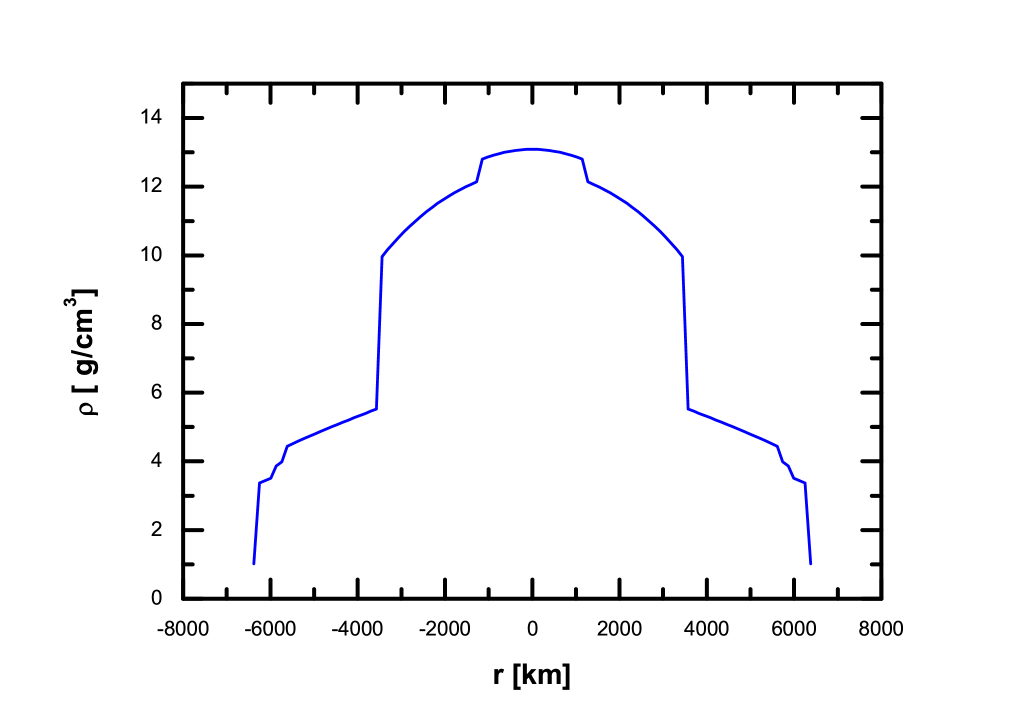
Figure 1: The Earth density profile PREM is plotted as a function radius $r$.

IV Results

In the standard picture of neutrino oscillation, the oscillation experiments with solar, atmospheric, reactor and accelerator neutrinos can be explained through the parametersAn:2013uza ; Ashie:2004mr ; Araki:2004mb

$$\Delta m^{2}_{21}=8.0\times 10^{-5}\mathrm{eV}^{2},\quad\theta_{12}=33.8^{\circ},\quad\quad\theta_{23}=45^{\circ}$$

$$\Delta m^{2}_{31}=3.2\times 10^{-3}\mathrm{eV}^{2},\quad\theta_{13}=8.8^{\circ}\quad\text{and}\quad\delta_{CP}=0,$$ (33)

with $\Delta m^{2}_{ij}=m^{2}_{i}-m^{2}_{j}$. Throughout our analysis we will be using the above neutrino parameters and the neutrinos in the energy range $1\,GeV\leq E_{\nu}\leq 100\,GeV$. Also we consider the normal neutrino mass hierarchy i.e. $m_{e}<m_{\mu}<m_{\tau}$ for the calculation of the oscillation probabilities of different neutrino flavors. The neutrinos propagating through the Earth will follow different trajectories depending on the zenith angle $\theta_{z}$ and is defined in ref.Petcov:1998su ; Chizhov:1999az , where $\theta_{z}=180^{\circ}$ corresponds to vertically up going neutrinos by crossing the diameter of the Earth, and $\theta_{z}=90^{\circ}$ corresponds to neutrinos coming from the horizon. To have maximum matter effect, we only consider the neutrinos which have $cos\theta_{z}=-1$ so that neutrinos can cross both mantle and core.

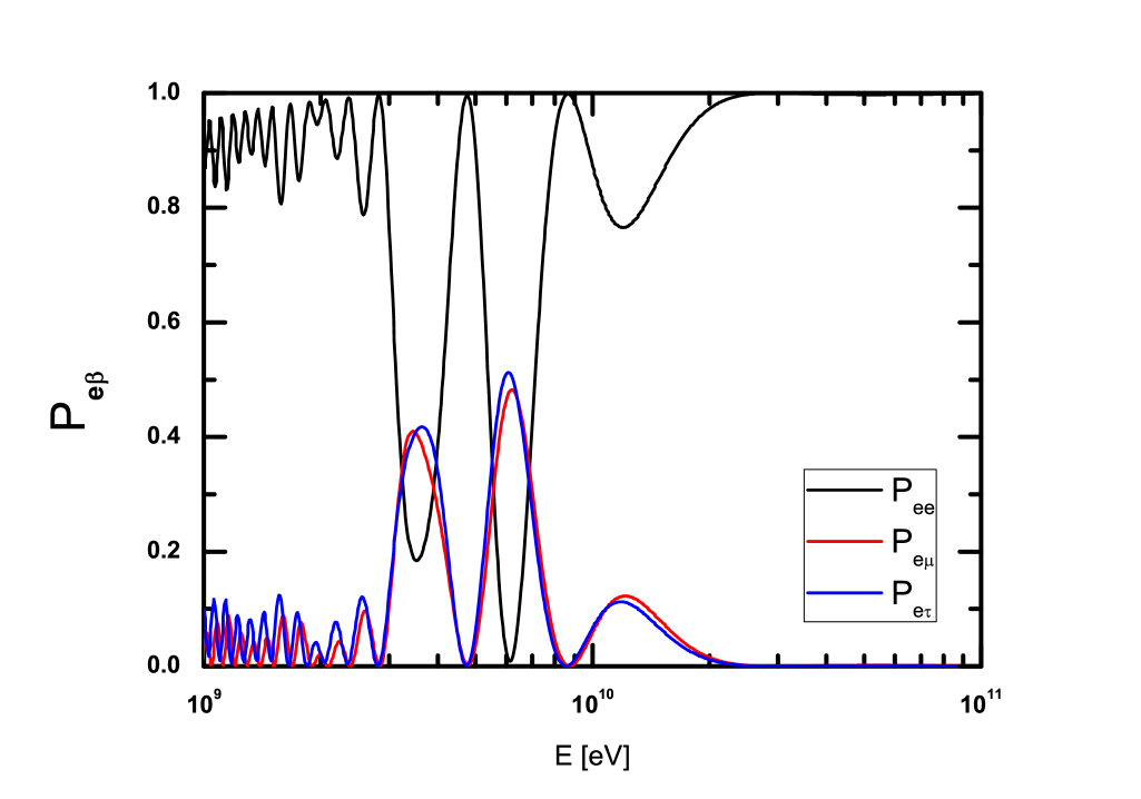
Figure 2: $P_{e\beta}$ as a function of neutrino energy $E_{\nu}$.

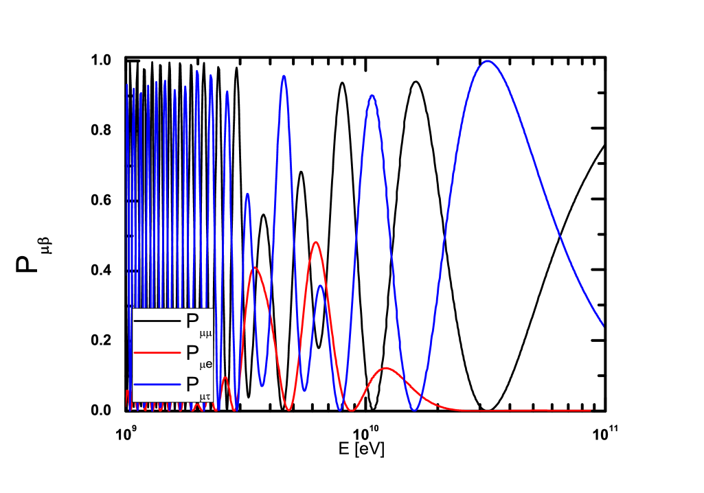
Figure 3: $P_{e\beta}$ as a function of neutrino energy $E_{\nu}$.

For $\nu_{e}$ oscillating to $\nu_{\mu}$ and $\nu_{\tau}$ we can clearly see three distinct resonance peaks in three different neutrino energies $E_{\nu}$ corresponding to three different densities $\rho$ of the Earth. The oscillation probability $P_{e\beta}$ is shown in Fig. 2. For $E_{\nu}=3.45$ GeV, the resonance takes place deep in the core where $\rho=11.5\,gm/cm^{3}$ at a depth of $\sim 2483$ km. The third peak is for $E_{\nu}=12.0$ GeV and the corresponding resonance density and the distance are respectively $3.4=gm/cm^{3}$ and 6112 km. These two peaks are clearly of MSW type because the resonance density and the resonance length exist for these neutrinos. On the other hand, for the second peak with $E_{\nu}=6.18$ GeV, the resonance density $\rho=6.6\,gm/cm^{3}$ does not exist in the Earth’s interior (Fig. 1). So this resonance can’t be of MSW type. This type of resonance is called parametric resonance which takes place if the variation of the matter density along the neutrino path is correlated in a certain way with the change of the oscillation phase Ermilova:1986 ; Akhmedov:1987nc ; Akhmedov:1998xq ; Liu:1998nb ; Akhmedov:2005yj . Below the first resonance peak ($E_{\nu}<3.45$ GeV) the probability is oscillatory in nature.

In Fig. 2 we have shown the $P_{ee}$, $P_{e\mu}$ and $P_{e\tau}$ for $1\,GeV\leq E_{\nu}\leq 100\,GeV$. It shows that for both the oscillations $\nu_{e}\leftrightarrow\nu_{\mu}$ and $\nu_{e}\leftrightarrow\nu_{\tau}$, the resonance peaks are at the same place for a given $E_{\nu}$. Beyond $\sim 20$ GeV the transition probabilities are very small which implies that the Earth’s matter does not play any significant role beyond this energy and the oscillation is purely due to the vacuum effect.

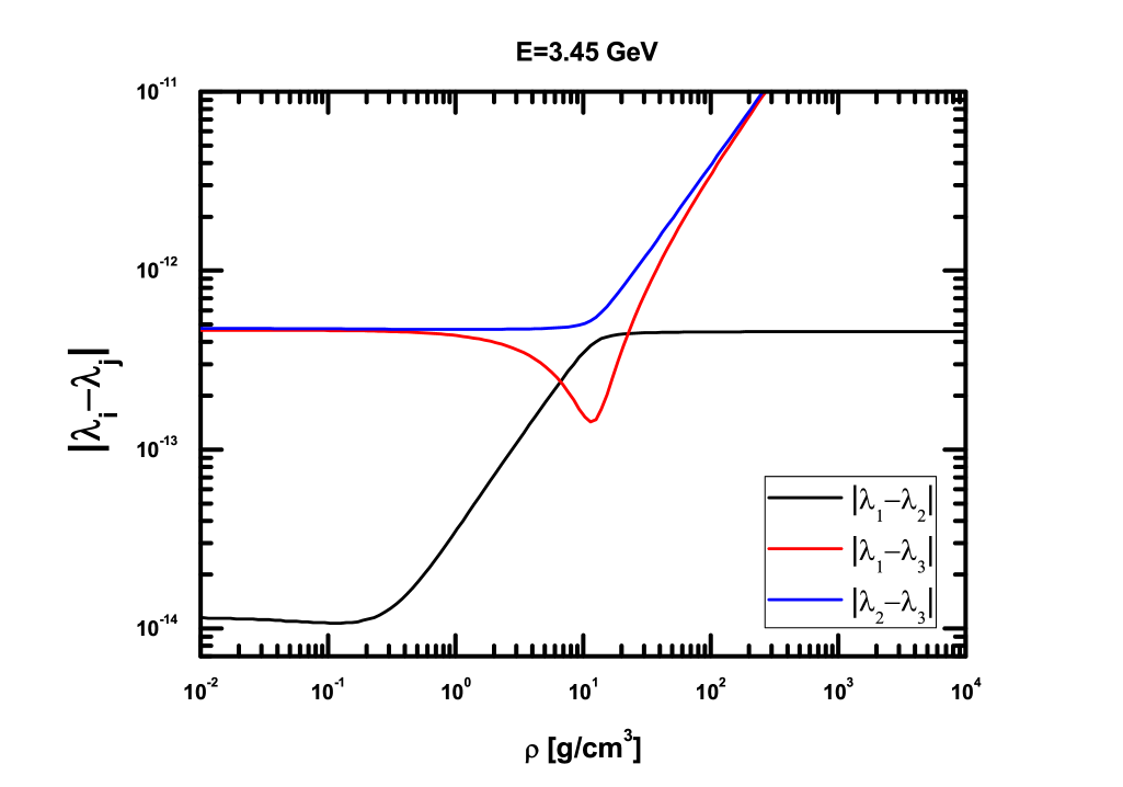
Figure 4: Neutrino energy difference is plotted as a function of density

In Fig. 3 we have shown the $P_{\mu\mu}$ and transition probabilities of muon neutrino to $\nu_{e}$ ($P_{\mu e}$) and to $\nu_{\tau}$ ($P_{\mu\tau}$). The three resonance peaks in $P_{\mu e}$ are clearly seen (red curve) but there is no resonant oscillation for $\nu_{\mu}\leftrightarrow\nu_{\tau}$ (blue curve). Above about $\sim 20$ GeV the $P_{\mu e}$ goes to zero and both $P_{\mu\mu}$ and $P_{\mu\tau}$ are out of phase by $180^{\circ}$. We observed that for $E_{\nu}>100$ GeV the $\nu_{\mu}$ does not oscillate to $\nu_{\tau}$ any more. The oscillation process $\nu_{\tau}\leftrightarrow\nu_{e}$ is same as $\nu_{e}\leftrightarrow\nu_{\mu}$, hence we do not discuss about it.

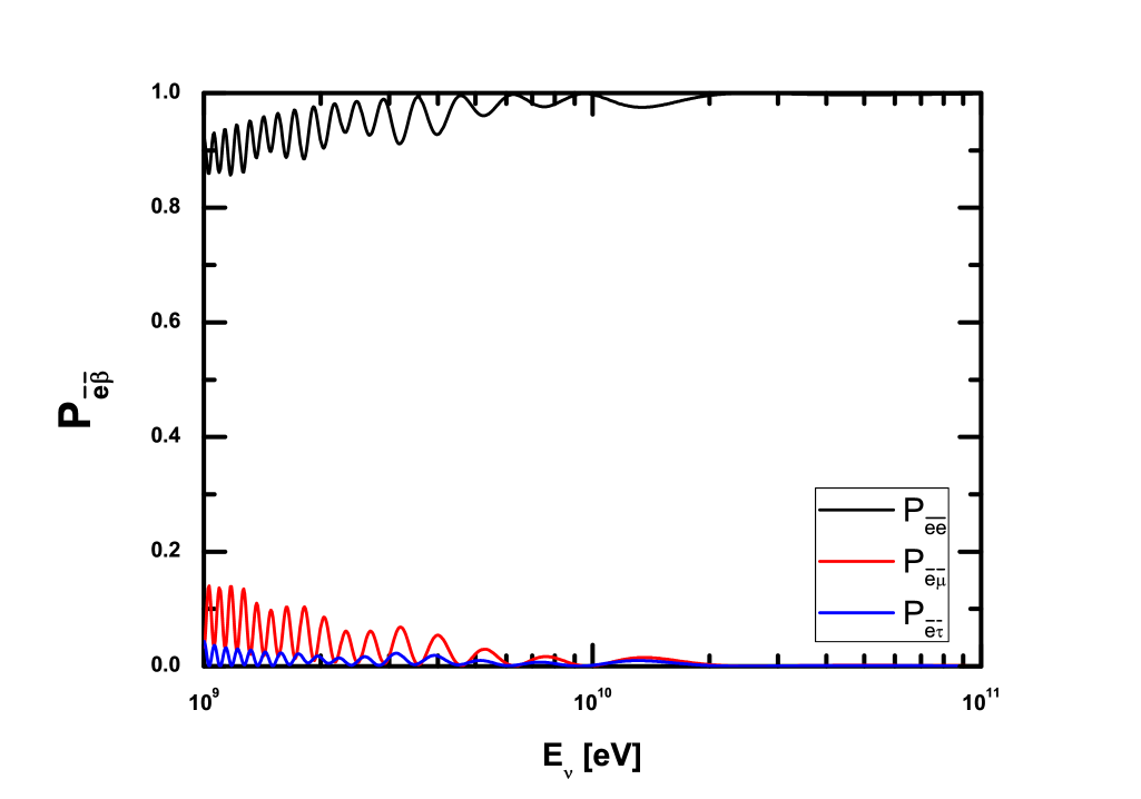
Figure 5: $P_{{\bar{\mu}}{\bar{\beta}}}$ as a function of $E_{\nu}$.

Due to the matter effect the energy eigenvalues of the neutrinos are given by $\lambda_{a}$ and the energy difference is related to the effective mass square difference as

$$|\lambda_{i}-\lambda_{j}|=\frac{|\Delta{\tilde{m}}^{2}_{ij}|}{2E_{\nu}}.$$ (34)

In Fig. 4 we have plotted $|\lambda_{i}-\lambda_{j}|$ as a function of Earth density $\rho$ for resonance neutrino energy $E_{\nu}=3.45$ GeV. It shows that, at the resonance density $\rho_{c}$, both $|\lambda_{1}-\lambda_{2}|$ and $|\lambda_{2}-\lambda_{3}|$ have the closest approach and at this point the neutrino mixing is maximal. Going from the resonance peak at 3.45 GeV to 12 GeV the resonance density decreases from 11.5 $gm/cm^{3}$ to 3.4 $gm/cm^{3}$.

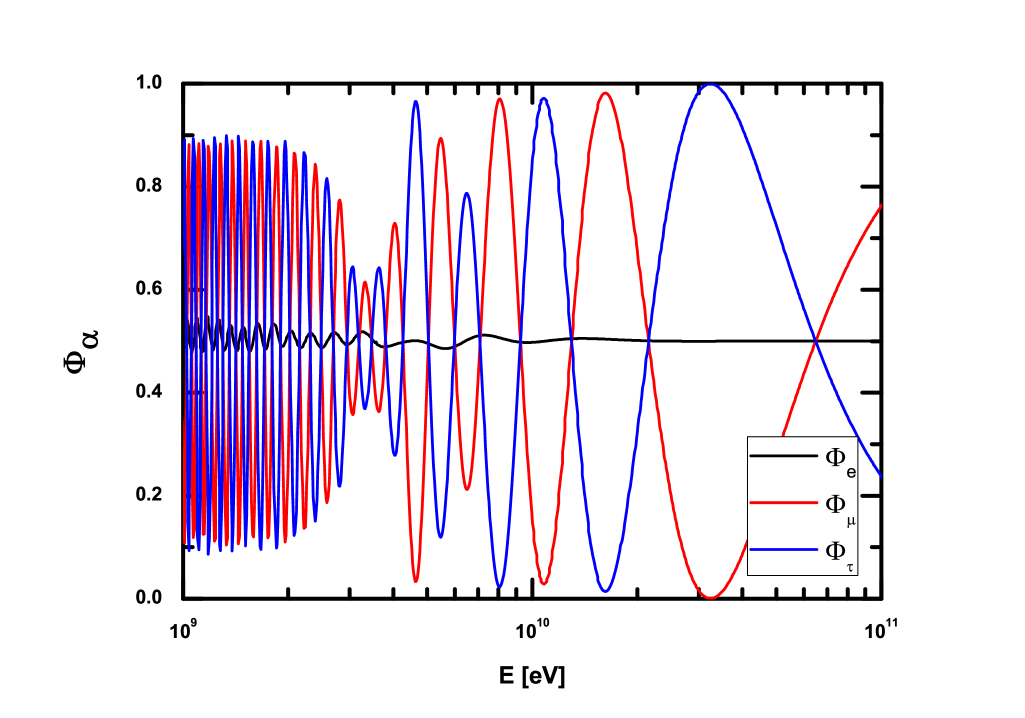
Figure 6: Neutrino flux at the IceCube detector when $\Phi^{0}_{\nu_{e}}:\Phi^{0}_{\nu_{\mu}}:\Phi^{0}_{\nu_{\tau}}=1:2:0$.

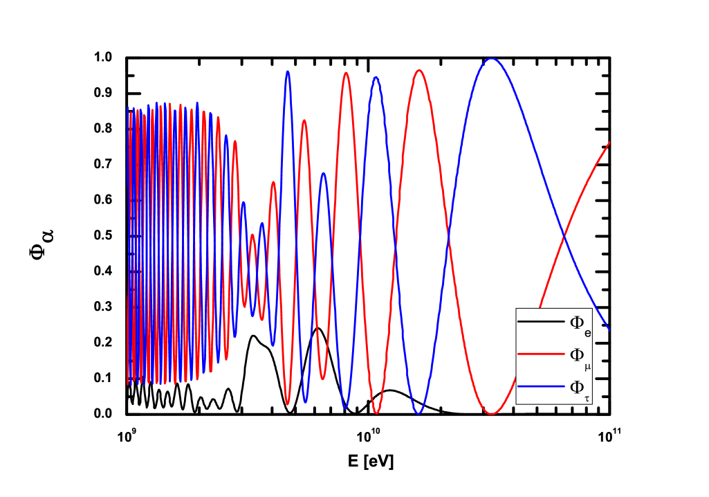
Figure 7: Neutrino flux at the IceCube detector when $\Phi^{0}_{\nu_{e}}:\Phi^{0}_{\nu_{\mu}}:\Phi^{0}_{\nu_{\tau}}=0:1:0$.

There are many uncertainties in determining the density profile of the Earth. The neutrino oscillations are not very sensitive to structures and gradients in the density profile if the length scale of these structures are shorter than the oscillation lengthWinter:2015zwx . However, we can treat the fluctuation in the density profile PREM by varying it around the mean value. By varying $\pm 10\%$ in the PREM density profile, Agarwalla et al.Agarwalla:2012uj have calculated the transition probability of $\nu_{e}\rightarrow\nu_{\mu}$ and survival probability of the process $\nu_{\mu}\rightarrow\nu_{\mu}$. It is shown that, in the sensitive region to density variation, the transition probability $P_{e\mu}$ is enhanced and $P_{\mu\mu}$ is reduced, and also the maxima and minima are shifted with respect to the negligible matter effects. As a consequence, the change in the density profile will shift the resonance position, thus modifying the number of events in different angular and energy bins. In our case also by varying the density we expect a similar behavior in resonance position which subsequently will change transition and survival probabilities of different neutrinos, but due to the fluctuation in the density, the average of these individual probabilities will not be very much different from their mean values. So, as a first approximation we consider the PREM without considering any fluctuation into it to understand the neutrino propagation and the resonance conditions in the few GeV energy regime.

We have also done the analysis for the oscillation of anti-neutrinos which are shown in Fig. 5. We observed that there is no resonant oscillation of the anti-neutrinos. As for anti-neutrinos the potential changes sign, it will never satisfy the resonance condition. However, if we consider the inverted mass hierarchy then due to the sign change we can have resonance for anti-neutrino oscillation but not for neutrino oscillation. In the low energy limit (between 1 to 10 GeV) for ${\bar{\nu}}_{e}\leftrightarrow{\bar{\nu}}_{\mu,\tau}$ oscillation, the oscillation of ${\bar{\nu}}_{e}$ to ${\bar{\nu}}_{\mu}$ is more preferable than to ${\bar{\nu}}_{\tau}$ which can be clearly seen from Fig. 5, but the oscillation probability is small. This is happening due to $\Delta m^{2}_{31}\gg\Delta m^{2}_{21}$. Above 10 GeV the oscillation ${\bar{\nu}}_{e}\leftrightarrow{\bar{\nu}}_{\mu,\tau}$ is suppressed. We observed that above $E_{\nu}>100$ GeV the ${\bar{\nu}}_{\mu}$ does not oscillate to ${\bar{\nu}}_{\tau}$ any more which is similar to the neutrino case discussed above.

The GeV energy neutrinos are produced mostly from the pion decay and have the standard flux ratio at the production point $\Phi^{0}_{\nu_{e}}:\Phi^{0}_{\nu_{\mu}}:\Phi^{0}_{\nu_{\tau}}=1:2:0$ ($\Phi^{0}_{\nu_{\alpha}}$ corresponds to the sum of neutrino and anti-neutrino flux at the source). Also when the muon is damped, the flux ratio at the source is $0:1:0$. The flux observed at a distance $L$ from the source is given by

$$\Phi_{\nu_{\alpha}}=\sum_{\beta}\Phi^{0}_{\nu_{\beta}}P_{\alpha\beta},\,\,\alpha,\beta=e,\,\mu,\,\tau.$$ (35)

When traveling in the Earth, the neutrinos will oscillates and the probability $P_{\alpha\beta}$ will be different for different flavors which is shown in Fig. 2. By using the above two neutrino flux ratios $1:2:0$ (standard) and $0:1:0$ (muon damped) at the source, we calculate the normalized observed flux ratio at the IceCube detector for the upward going neutrinos. For this calculation we don’t take into account the vacuum effect. Here our main aim is to calculate the observed flux ratios of the neutrinos at the detector for different flux ratios at the source without taking into account the vacuum oscillation when traversing the distance between the source and the Earth.

In Fig. 6 we observe that for the flux ratio $1:2:0$ at the source, the electron neutrino flux $\Phi_{\nu_{e}}$ is almost constant $\sim 0.5$ and the $\Phi_{\nu_{\mu}}$ and $\Phi_{\nu_{\tau}}$ oscillate between 0 and 1 averaging out to $0.5$. So for this case the observed flux ratio is found to be $1:1:1$. In Fig. 7 we have shown the muon damped scenario. For $E_{\nu}>\,20$ GeV the $\Phi_{\nu_{e}}\sim 0$ but average $\Phi_{\nu_{\mu}}\simeq\Phi_{\nu_{\tau}}=0.45$. Again for $E_{\nu}<20$ GeV there are three peaks in the normalized flux for $\Phi_{\nu_{e}}$ corresponding to three resonances as discussed before and shown in Figs. 2 and 3. In this case we always get $\Phi_{\nu_{e}}<\Phi_{\nu_{\mu}}\simeq\Phi_{\nu_{\tau}}$. Due to lower sensitivity of PINGU $\sim{\cal O}(1)$ GeV it can probe the resonance energy region $3\,GeV<E_{\nu}\leq\,12\,GeV$ very well. In the muon damped scenario, any transient source producing neutrinos in the few GeV energy range will be detected with a suppressed electron neutrino flux and enhanced muon and tau neutrino fluxes of equal strength if the Earth density profile is correct. However, due to the overwhelming atmospheric neutrino background in this energy range, it will be hard to detect these neutrinos unless the flux from the source is high.

V Discussion

Apart from atmospheric neutrinos, there are other astrophysical sources which can produce low energy GeV neutrinos. We used the formalism by Ohlsson and Snellman in a varying potential to calculate the active-active neutrino oscillation probability numerically by considering three active neutrino flavors and the realistic density profile PREM of the Earth. We observed that in the neutrino energy range $3\,GeV\leq E_{\nu}\leq\,12\,GeV$ three distinct resonances were observed in three different densities. However, the second resonance at an energy $E_{\nu}=6.18$ GeV corresponding to the density $6.6\,g/cm^{3}$ does not exit in the Earth interior. So this resonance is of non-MSW type but a parametric resonance. We also calculated the observed neutrino flux for these upward going neutrinos for standard scenario and the muon damped scenario taking into account the normal neutrino mass hierarchy. For standard scenario we obtained the observed flux ratio $1:1:1$ whereas for muon damped scenario we obtained $\Phi_{\nu_{e}}<\Phi_{\nu_{\mu}}\simeq\Phi_{\nu_{\tau}}$ for $E_{\nu}<20$ GeV and above this energy we obtained $\Phi_{\nu_{e}}\sim 0$, $\Phi_{\nu_{\mu}}\simeq\Phi_{\nu_{\tau}}=0.45$. The fluctuation in the density profile PREM can be considered to calculate the variation in the oscillation probabilities of different flavors. This change in density will change the position of resonances. However, as a first approximation, we consider the PREM without any fluctuation in it. The PINGU, which has a lower sensitivity will probably be able to probe this low energy range and shed more light on the MSW mechanism and also it can test the correctness of the Earth density profile PREM.

References

- (1) Y. Fukuda et al. [Super-Kamiokande Collaboration], Phys. Rev. Lett. 81, 1562 (1998) [hep-ex/9807003].
- (2) Y. Ashie et al. [Super-Kamiokande Collaboration], Phys. Rev. D 71, 112005 (2005) [hep-ex/0501064].
- (3) M. B. Smy et al. [Super-Kamiokande Collaboration], Phys. Rev. D 69, 011104 (2004) [hep-ex/0309011].
- (4) A. Gando et al. [KamLAND Collaboration], Phys. Rev. D 83, 052002 (2011) [arXiv:1009.4771 [hep-ex]].
- (5) F. P. An et al. [Daya Bay Collaboration], Chin. Phys. C 37, 011001 (2013) [arXiv:1210.6327 [hep-ex]].
- (6) M. G. Aartsen et al. [IceCube Collaboration], Science 342, 1242856 (2013) [arXiv:1311.5238 [astro-ph.HE]].
- (7) M. G. Aartsen et al. [IceCube Collaboration], Phys. Rev. Lett. 113, 101101 (2014) [arXiv:1405.5303 [astro-ph.HE]].
- (8) R. Abbasi et al. [IceCube Collaboration], Astropart. Phys. 35, 615 (2012) [arXiv:1109.6096 [astro-ph.IM]].
- (9) T. Palczewski [IceCube/PINGU Collaboration], “Neutrino Physics with the Precision IceCube Next Generation Upgrade (PINGU),” doi:10.3204/DESY-PROC-2014-04/84
- (10) T. P. Walker and D. N. Schramm, Phys. Lett. B 195, 331 (1987). doi:10.1016/0370-2693(87)90027-X.
- (11) T. K. Kuo and J. T. Pantaleone, Phys. Rev. Lett. 57, 1805 (1986).
- (12) A. Y. Smirnov, Yad. Fiz. 46, 1152 (1987).
- (13) S. T. Petcov and S. Toshev, Phys. Lett. B 187, 120 (1987).
- (14) T. P. Walker and D. N. Schramm, Phys. Lett. B 195, 331 (1987). doi:10.1016/0370-2693(87)90027-X
- (15) B. Jegerlehner, F. Neubig and G. Raffelt, Phys. Rev. D 54, 1194 (1996) doi:10.1103/PhysRevD.54.1194 [astro-ph/9601111].
- (16) T. Ohlsson and H. Snellman, Phys. Lett. B 474, 153 (2000).
- (17) T. Ohlsson and H. Snellman, J. Math. Phys. 41, 2768 (2000) [J. Math. Phys. 42, 2345 (2001)] [hep-ph/9910546].
- (18) T. Ohlsson and H. Snellman, Eur. Phys. J. C 20, 507 (2001).
- (19) T. Ohlsson and W. Winter, Phys. Lett. B 512, 357 (2001) doi:10.1016/S0370-2693(01)00731-6 [hep-ph/0105293].
- (20) T. Ohlsson, Phys. Scripta T 93, 18 (2001). doi:10.1238/Physica.Topical.093a00018
- (21) E. Sanroma and E. Palle, Astrophys. J. 744, 188 (2012) doi:10.1088/0004-637X/744/2/188 [arXiv:1110.1340 [astro-ph.EP]].
- (22) A. S. Dighe, M. Kachelriess, G. G. Raffelt and R. Tomas, JCAP 0401, 004 (2004) doi:10.1088/1475-7516/2004/01/004 [hep-ph/0311172].
- (23) E. K. Akhmedov, M. Maltoni and A. Y. Smirnov, JHEP 0806, 072 (2008) doi:10.1088/1126-6708/2008/06/072 [arXiv:0804.1466 [hep-ph]].
- (24) E. K. Akhmedov, M. Maltoni and A. Y. Smirnov, JHEP 0705, 077 (2007) doi:10.1088/1126-6708/2007/05/077 [hep-ph/0612285].
- (25) C. Rott, A. Taketa and D. Bose, Sci. Rep. 5, 15225 (2015) doi:10.1038/srep15225 [arXiv:1502.04930 [physics.geo-ph]].
- (26) L. Wolfenstein, Phys. Rev. D 17, 2369 (1978).
- (27) S. P. Mikheev and A. Y. Smirnov, Sov. J. Nucl. Phys. 42, 913 (1985) [Yad. Fiz. 42, 1441 (1985)].
- (28) G. M. Fuller, W. C. Haxton and G. C. McLaughlin, Phys. Rev. D 59, 085005 (1999) doi:10.1103/PhysRevD.59.085005 [astro-ph/9809164].
- (29) K. Takahashi, K. Sato, H. E. Dalhed and J. R. Wilson, Astropart. Phys. 20, 189 (2003) doi:10.1016/S0927-6505(03)00175-0 [astro-ph/0212195].
- (30) T. Yoshida, T. Kajino, H. Yokomakura, K. Kimura, A. Takamura and D. H. Hartmann, Phys. Rev. Lett. 96, 091101 (2006) doi:10.1103/PhysRevLett.96.091101 [astro-ph/0602195].
- (31) B. Dasgupta and A. Dighe, Phys. Rev. D 77, 113002 (2008) doi:10.1103/PhysRevD.77.113002 [arXiv:0712.3798 [hep-ph]].
- (32) H. Duan and A. Friedland, Phys. Rev. Lett. 106, 091101 (2011) doi:10.1103/PhysRevLett.106.091101 [arXiv:1006.2359 [hep-ph]].
- (33) S. Sahu and V. M. Bannur, Phys. Rev. D 61, 023003 (2000) [hep-ph/9806427].
- (34) P. Meszaros and E. Waxman, Phys. Rev. Lett. 87, 171102 (2001) doi:10.1103/PhysRevLett.87.171102 [astro-ph/0103275].
- (35) S. Razzaque, P. Meszaros and E. Waxman, Phys. Rev. Lett. 90, 241103 (2003) doi:10.1103/PhysRevLett.90.241103 [astro-ph/0212536].
- (36) S. Razzaque, P. Meszaros and E. Waxman, Phys. Rev. D 68, 083001 (2003) doi:10.1103/PhysRevD.68.083001 [astro-ph/0303505].
- (37) T. Kajino, T. Sasaqui, T. Yoshida and W. Aoki, Mod. Phys. Lett. A 23, 1409 (2008). doi:10.1142/S0217732308027783
- (38) S. Sahu and J. C. D’Olivo, Phys. Rev. D 71, 047303 (2005) [hep-ph/0502043].
- (39) S. Sahu, N. Fraija and Y. Y. Keum, Phys. Rev. D 80, 033009 (2009) [arXiv:0904.0138 [hep-ph]].
- (40) S. Razzaque, P. Meszaros and E. Waxman, Mod. Phys. Lett. A 20, 2351 (2005) doi:10.1142/S0217732305018414 [astro-ph/0509729].
- (41) S. Razzaque, P. Meszaros and E. Waxman, Phys. Rev. Lett. 93, 181101 (2004) Erratum: [Phys. Rev. Lett. 94, 109903 (2005)] doi:10.1103/PhysRevLett.93.181101, 10.1103/PhysRevLett.94.109903 [astro-ph/0407064].
- (42) O. Mena, I. Mocioiu and S. Razzaque, Phys. Rev. D 75, 063003 (2007) doi:10.1103/PhysRevD.75.063003 [astro-ph/0612325].
- (43) S. Razzaque and A. Y. Smirnov, JHEP 1505, 139 (2015) doi:10.1007/JHEP05(2015)139 [arXiv:1406.1407 [hep-ph]].
- (44) S. Razzaque and A. Y. Smirnov, JHEP 1003, 031 (2010) doi:10.1007/JHEP03(2010)031 [arXiv:0912.4028 [hep-ph]].
- (45) N. Senno, K. Murase and P. Mészáros, arXiv:1706.02175 [astro-ph.HE].
- (46) K. Murase and K. Ioka, Phys. Rev. Lett. 111, no. 12, 121102 (2013) doi:10.1103/PhysRevLett.111.121102 [arXiv:1306.2274 [astro-ph.HE]].
- (47) S. Sahu and B. Zhang, Res. Astron. Astrophys. 10, 943 (2010) [arXiv:1007.4582 [hep-ph]].
- (48) A. F. Osorio Oliveros, S. Sahu and J. C. Sanabria, Eur. Phys. J. C 73, 2574 (2013) [arXiv:1304.4906 [astro-ph.HE]].
- (49) K. Enqvist, K. Kainulainen and J. Maalampi, Nucl. Phys. B 349, 754 (1991).
- (50) M. Freund and T. Ohlsson, Mod. Phys. Lett. A 15, 867 (2000) [hep-ph/9909501].
- (51) W. Winter, Phys. Rev. D 72, 037302 (2005) doi:10.1103/PhysRevD.72.037302 [hep-ph/0502097].
- (52) S. K. Agarwalla, T. Li, O. Mena and S. Palomares-Ruiz, arXiv:1212.2238 [hep-ph].
- (53) W. Winter, Nucl. Phys. B 908, 250 (2016) doi:10.1016/j.nuclphysb.2016.03.033 [arXiv:1511.05154 [hep-ph]].
- (54) A. M. Dziewonski, D. L. Anderson, Preliminary reference Earth model. Phys. Earth Planet. Inter. 25 297-356.
- (55) S. Gao and P. Meszaros, Phys. Rev. D 85, 103009 (2012) [arXiv:1112.5664 [astro-ph.HE]].
- (56) I. Bartos, A. M. Beloborodov, K. Hurley and S. Márka, Phys. Rev. Lett. 110, no. 24, 241101 (2013) doi:10.1103/PhysRevLett.110.241101 [arXiv:1301.4232 [astro-ph.HE]].
- (57) K. Murase, K. Kashiyama and P. Mészáros, Phys. Rev. Lett. 111, 131102 (2013) doi:10.1103/PhysRevLett.111.131102 [arXiv:1301.4236 [astro-ph.HE]].
- (58) P. Meszaros and M. J. Rees, Astrophys. J. 541, L5 (2000) doi:10.1086/312894 [astro-ph/0007102].
- (59) J. N. Bahcall and P. Meszaros, Phys. Rev. Lett. 85, 1362 (2000) doi:10.1103/PhysRevLett.85.1362 [hep-ph/0004019].
- (60) K. Murase, B. Dasgupta and T. A. Thompson, Phys. Rev. D 89, no. 4, 043012 (2014) doi:10.1103/PhysRevD.89.043012 [arXiv:1303.2612 [astro-ph.HE]].
- (61) A. M. Atoyan and C. D. Dermer, New Astron. Rev. 48, 381 (2004) doi:10.1016/j.newar.2003.12.046 [astro-ph/0402646].
- (62) V. D. Barger, K. Whisnant, S. Pakvasa and R. J. N. Phillips, Phys. Rev. D 22, 2718 (1980).
- (63) C. W. Kim and W. K. Sze, Phys. Rev. D 35, 1404 (1987).
- (64) H. W. Zaglauer and K. H. Schwarzer, Z. Phys. C 40, 273 (1988).
- (65) S. T. Petcov, Phys. Lett. B 191, 299 (1987).
- (66) H. Lehmann, P. Osland and T. T. Wu, Commun. Math. Phys. 219, 77 (2001).
- (67) K. Varela, S. Sahu, A. F. O. Oliveros and J. C. Sanabria, Eur. Phys. J. C 75, no. 6, 289 (2015) [arXiv:1411.7992 [astro-ph.HE]].
- (68) Y. Ashie et al. [Super-Kamiokande Collaboration], Phys. Rev. Lett. 93, 101801 (2004) [hep-ex/0404034].
- (69) T. Araki et al. [KamLAND Collaboration], Phys. Rev. Lett. 94, 081801 (2005) [hep-ex/0406035].
- (70) S. T. Petcov, Phys. Lett. B 434, 321 (1998) doi:10.1016/S0370-2693(98)00742-4, 10.1016/S0370-2693(98)01437-3 [hep-ph/9805262].
- (71) M. V. Chizhov and S. T. Petcov, Phys. Rev. Lett. 83, 1096 (1999) doi:10.1103/PhysRevLett.83.1096 [hep-ph/9903399]. HEP :: Search :: Help :: Terms of use :: Privacy policy Powered by Invenio v1.1.2+ Problems/Questions to feedback@inspirehep.net
- (72) V. K. Ermilova, V. A. Tsarev, V. A. Chechin and Kr. Soob, Fiz. Short Notices of the Lebedev Institute 5, 26 (1986).
- (73) E. K. Akhmedov, Sov. J. Nucl. Phys. 48, 382 (1988) [Yad. Fiz. 48, 599 (1988)].
- (74) E. K. Akhmedov, A. Dighe, P. Lipari and A. Y. Smirnov, Nucl. Phys. B 542, 3 (1999) doi:10.1016/S0550-3213(98)00825-6 [hep-ph/9808270].
- (75) Q. Y. Liu, S. P. Mikheyev and A. Y. Smirnov, Phys. Lett. B 440, 319 (1998) doi:10.1016/S0370-2693(98)01102-2 [hep-ph/9803415].
- (76) E. K. Akhmedov, M. Maltoni and A. Y. Smirnov, Phys. Rev. Lett. 95, 211801 (2005) doi:10.1103/PhysRevLett.95.211801 [hep-ph/0506064].