The Lindley paradox in optical interferometry

Abstract

The so-called Lindley paradox is a counterintuitive statistical effect where the Bayesian and frequentist approaches to hypothesis testing give radically different answers, depending on the choice of the prior distribution. In this paper we address the occurrence of the Lindley paradox in optical interferometry and discuss its implications for high-precision measurements. In particular, we focus on phase estimation by Mach-Zehnder interferometers and show how to mitigate the conflict between the two approaches by using suitable priors.

I Introduction

Interferometric setups are at the heart of several high-precision measurement schemes, ranging from gravitational wave-detectors to laser gyroscopes and clocks synchronization protocols. In particular, a direct detection of gravitational waves is supposed to come from laser-interferometric detectors rev80 ; rev14 ; rev08 , where they induce a measurable variation of the optical paths of the light beams traveling along the arms of an interferometric setup.

Inteferometers are usually employed to detect small perturbations, so that detectors must be able to measure distance changes with remarkable precision and any source of noise must be carefully removed. Indeed, recent technological advances in precision lasers, vacuum technology and optical systems had made it possible to greatly reduce classical noise. However, an unavoidable constraint to the precision with which optical signals can be measured arises from the quantum nature of the electromagnetic field. The so-called standard quantum limit (SQL) bra92 , sometimes also referred to as shot noise, results as a consequence of the uncertainty relations existing for the quantum field operators.

A way to partially circumvent the effects of quantum fluctuations and increase interferometric precision is to exploit the use of squeezed light cav81 ; bon84 ; yur86 or other nonclassical states of light hol93 ; sun08 , also in the presence of inefficient detectors par95 . The implementation of squeezing-enhancement techniques in interferometric detectors has been a great challenge: after a large number of experimental and theoretical studies it has now became possible to take advantage of squeezing geo600 ; berni15 so that the next generation of interferometers will be equipped with quantum technologies.

In order to effectively exploit the potential improvements offered by quantum signals, the statistical analysis of the data should be refined as well. In this context, the key point is to improve the ability of discriminating whether a signal contains instrumental noise only or also a trace of a signal. This problem, which arises in the form of a hypothesis testing problem par97 , might be conveniently studied by means of Bayesian inference hol93 ; pez07 ; pez08 ; oli09 ; ber09 ; gen11 ; gen12 ; oli13 . However, a Bayesian approach may be challenging since it requires the full knowledge of the system under consideration in order to properly introduce a suitable prior, together with a high computational power. Indeed, in a Bayesian framework we have to provide explicit models of the signal induced by a perturbation to achieve, after specifying our prior knowledge, the odds ratio of the detection hypothesis over the null hypothesis, corresponding to absence of signal. In this context, it may happen that the lack of knowledge about the system increases the false alarm probability. In other words, the posterior odds may favor the alternative hypothesis, i. e. presence of perturbations, even if no signals are actually present in data. In particular, when a diffuse prior distribution is taken, a Bayesian approach to hypothesis testing leads to conflicting evidences compared to a frequentist approach. Such a counterintuitive situation was studied by Jeffrey jef48 together with Lindley, who first referred to this disagreement as a statistical paradox lin57 .

The relevance of Bayesian analysis in interferometry has been recognized since a long time hol93 ; hra96 . The interest raised for at least three reasons. On the one hand, common interferometric estimators are known to achieve optimal performances only at a specific working point cav81 ; dow98 , thus resulting in interferometric protocols that do not allow the measurement of arbitrary phase shifts. Besides, in order to estimate small fluctuations around the working point, the interferometer has to be actively stabilized by the addition of some feedback mechanism fed96 . Finally, Bayesian estimators have been shown to achieve the asymptotic regime, where they saturate the Cramer-Rao bound, already with few measurements berni15 ; oli09 ; ber09 ; gen11 , thus representing a convenient choice in any setting where resources are limited or the samples involved in the interferometric setup are fragile.

In this work we address in details the occurrence of the Lindley paradox lin77 ; sha82 in the analysis of data coming from optical interferometry. The importance of the topic seats in the fact that often, e.g. in the framework of gravitational antennas, each event is of great relevance and should be analyzed in the most refined way as the above mentioned debate concerning cosmological measurements suggests. More generally, it is often the case that besides the estimation of small fluctuations, interferometric measurements are involved in monitoring a given physical configuration, where the information coming from the experimental data is exploited to statistically discriminate between two hypothesis wis09 ; kum11 ; rei11 ; kir14 ; fen14 . Here, we first consider homodyne detection, then classical-like Mach-Zehnder (MZ) interferometer, and finally we consider the case of squeezed-enhanced quantum interferometers. For the MZ interferometer we start from the analysis of the ideal case wherein the detectors are perfectly efficient, and a widespread prior is assumed, and then proceed by assessing the realistic case where inefficient detectors and a concentrated prior distribution is employed. As we will see, the Lindley paradox may indeed arise in optical interferometry. Here we show how to mitigate the conflict between the Bayesian and frequentist approaches by using suitable priors.

The paper is organized as follows. In Sec. II we introduce the notation and illustrate how and when the paradox can arise. In Sec. III we discuss phase estimation by homodyne detection as a suitable example to illustrate the statistical analysis step by step. In Sec. IV we analyze in details the occurrence of the paradox in optical interferometry, whereas Section V closes the paper with some concluding remarks.

II The Lindley Paradox

Let us consider a random variable $X$ distributed according to a Gaussian distribution of unknown mean $\phi$ and known variance $\sigma^{2}$. Suppose that we want to test a sharp null hypothesis $H_{0}$, corresponding to the prediction $\phi=\phi_{0}$, against the alternative hypothesis $H_{1}$, corresponding to the diffuse prediction $\phi\neq\phi_{0}$. In a Bayesian framework this is done assigning a priori a probability $p\left(H_{i}\right)$ and a prior distribution $\pi_{i}\left(\phi\right)$ to any hypothesis $H_{i}$ taken into account. Let us denote the priors by $p\left(H_{0}\right)=z_{0}$ and $p\left(H_{1}\right)=1-z_{0}$, with $z_{0}\in[0,1]$. Besides, we take $\pi_{0}\left(\phi\right)$ to be a Dirac’s delta function since the null hypothesis involves a single parameter value. As for the probability density $\pi_{1}(\phi)$, concerning the alternative hypothesis, we assume a normal distribution with variance $\tau^{2}$. That being said, the posterior probability $\bar{z}_{0}$ that the outcome $X=x$ provides evidence of $\phi=\phi_{0}$ , i. e. confirms the null hypothesis, is evaluated via Bayes’ theorem, which yields (see A):

$$\bar{z}_{0}=p\left(\phi=\phi_{0}|x\right)=\left\{1+\frac{1-z_{0}}{z_{0}}\frac{p\left(x|\phi\neq\phi_{0}\right)}{p\left(x|\phi=\phi_{0}\right)}\right\}^{-1}\,.$$ (1)

In order to illustrate the occurrence of the Lindley paradox, let us consider the simple case where $\phi_{0}=0$ and $\sigma=1$, where we have (see A for the general case)

$$\bar{z}_{0} =p\left(\phi=\phi_{0}|x\right)$$

$$=\left\{1+\frac{1-z_{0}}{z_{0}}\frac{1}{\sqrt{1+\tau^{2}}}\exp\left[\frac{x^{2}\tau^{2}}{2\left(1+\tau^{2}\right)}\right]\right\}^{-1},$$ (2)

which goes to $1$ as $\tau$ goes to infinity, no matter the value of the outcome $x$ and of the prior probability $z_{0}$. In other words, when the prior distribution for the alternative hypothesis becomes non-informative (i.e. approaches a flat distribution), a Bayesian approach awards high odds to the null hypothesis even if the observed value is several standard deviation away from $\phi_{0}$. This is clearly in contrast with the predictions that any frequentist approach based on sampling theory may provide, not speaking of common sense.

The nature of the paradox, actually the lack of any paradox, has been extensively analyzed lin77 ; sha82 and we are not going to discuss the situation from a statistical point of view, which would be beyond the scope of our analysis. We limit ourselves to notice that the disagreement between the two approaches is basically caused by the fact that the frequentist approach tests one hypothesis without reference to the other, whereas Bayesian analysis assess them as alternative one to each other, looking for the one in better agreement with the observations. We also point out that the paradox is of great generality since the key point for its appearance is the use of a diffuse prior distribution. In the following sections, we will exhibit three situation of physical interest where the data analysis naturally involves the assignment of a prior, such that a discussion about the occurrence of the paradox is worthwhile.

III Phase estimation by homodyne detection

Homodyne detection is a measurement scheme where the observed mode of the field interferes with a reference mode, thus providing indirect information about its phase. The device is illustrated schematically in Fig. (1).

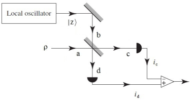
Figure 1: Schematic diagram of homodyne detection scheme

The field to be measured, prepared in an arbitrary state $\rho$ of a single-mode $a$, is mixed with the field produced by an intense laser, i.e. with a highly excited coherent state $\left|z\right\rangle$, with $z=\left|z\right|e^{i\phi}\in\mathbb{C}$. Two detectors measure the photocurrents $i_{c}$ and $i_{d}$, while a differential amplifier determines the homodyne photocurrent $H$, i.e. the rescaled difference photocurrent $\hat{H}=(\hat{i}_{c}-\hat{i}_{d})/\sqrt[2]{|}z|$. In the limit of large $|z|$ it turns out that homodyne detection provides the measurement of the quadrature operator $\hat{\chi}_{\phi}$ given by:

$$\hat{\chi}_{\phi}=\frac{\hat{a}^{\dagger}e^{i\phi}+\hat{a}e^{-i\phi}}{\sqrt{2}}\,.$$ (3)

We point out that the device works properly only if the incoming fields occupy the same spatial mode, have the same frequency $\omega$ and are co-polarized. Besides, note that our description refers to ideal photodetectors with quantum efficiency equal to $1$. This being said, we address homodyne detection as a tool to establish whether the phase of a given initial field has been perturbed or not, e. g. due to interaction with the environment. In particular, we consider a squeezed state $\left|\alpha,\lambda\right\rangle$, with $\alpha=\left|\alpha\right|e^{i\theta}$, $\lambda=re^{i\varphi}\in\mathbb{C},r>0$. That is, we take the impinging beam to be in a pure state given by:

$$\left|\psi_{0}\right\rangle=\left|\alpha,\lambda\right\rangle=\hat{D}(\alpha)\hat{S}(\lambda)\left|0\right\rangle\,,$$ (4)

where $\hat{S}(\lambda)=\exp(-\frac{\lambda}{2}\hat{a}^{\dagger 2}+\frac{\lambda^{*}}{2}\hat{a}^{2})$ and $\hat{D}(\alpha)=\exp(-\alpha\hat{a}^{\dagger}+\alpha^{*}\hat{a})$ are unitary operators, namely the squeezing operator and the displacement operator, whose action in the phase space defined by the observables $\hat{\chi}_{\phi}$ and $\hat{\chi}_{\phi+\frac{\pi}{2}}$ is, respectively, an hyperbolic rotation and a translation. Besides, we assume that the interaction with the environment results in a phase shift expressed by the evolution operator $\hat{U}_{I}=\exp(-i\hat{a}^{\dagger}\hat{a}\beta)$, with $\beta\in[0,2\pi]$. The final state $\left|\psi\right\rangle$, impinging on the semi-reflecting mirror, is readily obtained using the BCH formulas, which yield:

$$\left|\psi\right\rangle=\hat{U}_{I}\left|\psi_{0}\right\rangle=\exp(-i\hat{a}^{\dagger}\hat{a}\beta)\left|\alpha,\lambda\right\rangle=\left|\alpha e^{-i\beta},\lambda e^{-2i\beta}\right\rangle.$$ (5)

The distribution $P_{\alpha,\lambda}(\chi_{\phi})$ of the outcomes of repeated measurements of $\hat{\chi}_{\phi}$ performed on radiation prepared in state $\left|\psi\right\rangle$ is a Gaussian with expectation value $\bar{\chi}_{\phi}$ and variance $\sigma^{2}_{\chi}$ given by:

$$\bar{\chi}_{\phi}=\left\langle\psi\left|\hat{\chi}_{\phi}\right|\psi\right\rangle=\frac{1}{\sqrt{2}}\left(\alpha e^{-i(\phi+\beta)}+\alpha^{*}e^{i(\phi+\beta)}\right)\,,$$ (6)

$$\sigma^{2}_{\chi} =\left\langle\psi\left|\hat{\chi}_{\phi}^{2}\right|\psi\right\rangle-\left\langle\psi\left|\hat{\chi}_{\phi}\right|\psi\right\rangle^{2}=$$

$$=\frac{1}{2}\left[e^{2r}\sin^{2}\left(\phi+\beta-\frac{\varphi}{2}\right)+e^{-2r}\cos^{2}\left(\phi+\beta-\frac{\varphi}{2}\right)\right]\,.$$ (7)

The above equations lead us to conclude that we shall check whether the outcomes of measurements by means of homodyne detection are consistent with the null hypothesis $\beta=\beta_{0}=0$ in order to establish whether the initial state $\left|\psi_{0}\right\rangle$ has been perturbed or not. Without loss of generality, we focus on a specific example and set $\theta=0$, $\varphi=0$, corresponding to an input amplitude-squeezed state. We may also fix the quadrature component to be measured: for the sake of simplicity we take $\phi=0$. In these conditions, Eqs (6, 7) becomes

$$\bar{\chi}_{0}\left(\beta\right) =|\alpha|\sqrt{2}\cos\beta=\bar{\chi}_{0}\left(\beta\right),$$ (8)

$$\sigma_{\chi}^{2}\left(\beta\right) =\frac{1}{2}[e^{2r}\sin^{2}\beta+e^{-2r}\cos^{2}\beta]\,.$$ (9)

Let us now suppose that a run returns an outcome $q=\bar{\chi}_{0}+t\cdot\sigma_{\chi}$, with $t\in\mathbb{R}$. In agreement with a standard sampling-theory test based on the value of $t$ we shall conclude that if $q$ is several $\sigma_{\chi}$ from $\bar{\chi}_{0}$ the null hypothesis is to be rejected: we have to say that a phase shift occurred and the state has been indeed perturbed. In order to provide a Bayesian assessment for $H_{0}$ we set a value for the prior probability, say $z_{0}=0.9$, and distribute uniformly the remainder probability $1-z_{0}$ over the interval $I=\left[-\pi,\pi\right]$, where the phase may take values. On one hand, we are allowed to set such a high value for $z_{0}$ under the assumption that we are leading an experiment in optimal conditions, any source of noise being taken into account. On the other hand, the choice of a flat prior should not be surprising since we have no idea about the dynamics of a possible interaction: we are equally (un)expected to measure a small or a large value for the phase shift. Eventually, the posterior probability $\bar{z}_{0}$ that $\beta=\beta_{0}=0$ is is evaluated by the Bayes theorem:

$$\bar{z}_{0}=\left\{1+\frac{1-z_{0}}{z_{0}}\frac{p\left(q|\beta\neq\beta_{0}\right)}{p\left(q|\beta=\beta_{0}\right)}\right\}^{-1},$$ (10)

where

$$p\left(q|\beta=\beta_{0}\right)=\frac{1}{\sqrt{2\pi\sigma_{\chi}^{2}\left(0\right)}}\exp\left[-\frac{q^{2}}{2\sigma_{\chi}^{2}\left(0\right)}\right],$$ (11)

$$p\left(q|\beta\neq\beta_{0}\right)=\int_{I}d\beta\>\frac{1}{\sqrt{2\pi\sigma_{\chi}^{2}\left(\beta\right)}}\exp\left[-\frac{\left(q-|\alpha|\sqrt{2}\cos\beta\right)^{2}}{2\sigma_{\chi}^{2}\left(\beta\right)}\right].$$ (12)

Note that the value of $\bar{z}_{0}$ only depends on the value $q$ of the outcome: we expect that the bigger is the difference $q-\bar{\chi}_{0}$, the smaller the posterior probability $\bar{z}_{0}$. In order to give a numerical estimate let us set $|\alpha|=10$ and $r=1$, i.e. we consider a squeezed state with one hundred photons, where only about $1\%$ of the total energy is employed in squeezing. Recalling that the null hypothesis corresponds to the condition $\beta=\beta_{0}=0$ we get $\bar{\chi}_{0}\left(0\right)=14.14$ and $\sigma_{\chi}^{2}\left(0\right)=0.07$ . By explicit calculations one can check that for $\left|q-\bar{\chi}_{0}\left(0\right)\right|\leq 4\sigma_{\chi}\left(0\right)$ the posterior probability is still over $50\%$: a Bayesian approach leads us to conclude that no phase perturbation actually occurred. That is, if $2\sigma_{\chi}\left(0\right)\leq\left|q-\bar{\chi}_{0}\left(0\right)\right|\leq 4\sigma_{\chi}\left(0\right)$ the Bayesian approach provides conflicting evidence with respect to the values obtained by a sampling test: we are in presence of the paradox.

The key point, in the present case as well as in the situation illustrated by Lindley, is that the prior is taken to be flat. To this regard we remark that despite this assumption is somehow consistent from a physical perspective, in practice it turns out that outcomes being several $\sigma_{\chi}\left(0\right)$ from the expectation value are associated to statistical fluctuations and the null hypothesis keeps on overwhelming any alternative. For this reason we shall rather conclude that the Bayesian approach is somehow misleading if a scarce information about the prior distributions is available, whereas a sampling-theory test better accounts what is really happening.

Since our main goal is to address the occurrence of the Lindley paradox in interferometry we will not go further in the discussion of this case. We only notice that here we have a physical example where the paradox unavoidably arises, the assumptions being consistent with the dynamics of the system. From a practical point of view, we notice that the characterization and the calibration of homodyne detectors is one of the building blocks for the robust implementation of quantum tomography of the radiation field reh04 .

IV Phase Estimation with Mach-Zehnder Interferometry

In the present section we consider the linear MZ interferometer, that allows one to monitor a classical phase parameter via photon counting measurements. A schematic diagram of the detector is shown in Fig. 2.

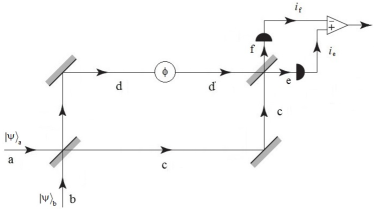
Figure 2: Schematic diagram of a Mach-Zehnder interferometer.

Two modes of the radiation field enters the interferometer through a first beam splitter, then a phase difference $\phi$ is inserted between the beams and, finally, the two fields exit through a second beam splitter. The number of photons in each mode is detected by means of two photodetectors of quantum efficiency $\eta$ that measure the photocurrents $i_{f}$ and $i_{e}$; a differential amplifier eventually determines the difference photocurrent, whose possible values correspond to the eigenvalues of the Hermitian operator

$$\hat{D}(\phi)=\eta\left(\hat{f}^{\dagger}\hat{f}-\hat{e}^{\dagger}\hat{e}\right)\,$$ (13)

which is a normalized version of the integrated photocurrent. It can be expressed in terms of the input fields as follows:

$$\hat{D}(\phi)=\eta\left[\left(\hat{a}^{\dagger}\hat{a}-\hat{b}^{\dagger}\hat{b}\right)\cos\phi+i\left(\hat{b}^{\dagger}\hat{a}-\hat{a}^{\dagger}\hat{b}\right)\sin\phi\right].$$ (14)

From the above equation it is clear that measurements of the difference photocurrent at the output allows one to assess variations of the phase difference $\phi$. In particular, from a linear error propagation theory one obtains the following expression for the sensitivity $\Delta\phi$ of the device:

$$\Delta\phi=\sqrt{\left\langle\hat{D}^{2}(\phi)\right\rangle-\left\langle\hat{D}(\phi)\right\rangle^{2}}\;\left|\frac{\partial}{\partial\phi}\left\langle\hat{D}(\phi)\right\rangle\right|_{\phi=\phi_{0}}^{-1},$$ (15)

which depends from the initial value $\phi_{0}$ and the expectation value $\left\langle\hat{D}(\phi)\right\rangle$. If any perturbations changes the length of the two arms of the interferometer, the optical paths covered by the light beams is altered. As a consequence, the phase difference $\phi$ will vary and so will do the outcomes of measurements of the operator $\hat{D}$: once the system has been set in a proper initial working point $\phi_{0}$ an outcome $\phi\neq\phi_{0}$ shall be associated to a displacement. Hence, the data analysis consists of assessing the probability that an outcome $d$ confirms the null hypothesis $H_{0}$, corresponding to no phase variation, or the alternative hypothesis $H_{1}$ that $\phi\neq\phi_{0}$. In this context, we discuss the possibility of coming across the Lindley paradox, paying particular attention to the conditions in which it can arise.

IV.1 Coherent light interferometry

At first, we consider a classical-like MZ interferometer fed by an input state of the form $\left|\psi\right\rangle=\left|\alpha\right\rangle\left|0\right\rangle$ where $\alpha=\left|\alpha\right|e^{i\theta}\in\mathbb{C}$. In this case, the outcomes $d$ of measurements of the operator $\hat{D}$ are distributed according to a Skellam distribution ske46 :

$$p_{\phi}(d)=e^{-\eta\left|\alpha\right|^{2}}\left(\frac{1+\cos\phi}{1-\cos\phi}\right)^{\frac{d}{2}}I_{\left|d\right|}\left(\eta\left|\alpha\right|^{2}\sin\phi\right),$$ (16)

where $I_{k}(z)$ is the modified Bessel function of the first kind. The mean value $\bar{d}_{\phi}$ and variance $\sigma_{d}^{2}$ of the above distribution are given by

$$\bar{d}_{\phi}=\left\langle\hat{D}(\phi)\right\rangle=\eta\left|\alpha\right|^{2}\cos\phi\,,$$ (17)

$$\sigma_{d}^{2}=\Delta^{2}\hat{D}=\eta\left|\alpha\right|^{2}.$$ (18)

This result may be easily understood recalling that the number of photons contained in a coherent state follows a Poissonian statistics and that the Skellam distribution provides the probability density of the difference between two Poisson variates. It is easy to see that for the given input state $\left|\psi\right\rangle$ the minimum value of $\Delta\phi$ is obtained for $\phi_{0}=\frac{\pi}{2}$. Therefore, we assume the interferometer to be set in this optimal working point (corresponding to a null mean value $\bar{d}_{\frac{\pi}{2}}=0$).

We now suppose that a trial results in the outcome $d$ of the difference photocurrent, that we represent as $d=\bar{d}_{\frac{\pi}{2}}+t\cdot\sigma_{d}=t\cdot\sigma_{d}$, with $t\in\mathbb{R}$. According to a standard sampling-theory test $d$ is to be associated to a displacement induced by a perturbation if its value is several $\sigma_{d}$ from $0$. In this event we shall reject the null hypothesis $H_{0}$. On the other side, in order to give a Bayesian assessment to $H_{0}$ we assign a probability $z_{0}$ to the null hypothesis and distribute the remainder over the interval $I=\left[0,\pi\right]$ where we expect the phase to vary. Assuming to deal with rare events we take $z_{0}=0.99$, i. e. we assume that almost only $1$ event out of $100$ is to be associated to an incoming perturbation rather than to a random error. With respect to the prior distribution for the alternative hypothesis we initially consider a situation where no information about the signal is available so that a flat prior results a proper choice. At this point we can compute the posterior probability $\bar{z}_{0}$ given $\phi=\phi_{0}=\frac{\pi}{2}$ by Eq. (10), where $\beta$ is to be substituted with $\phi$ and the probability densities take the following expressions:

$$p\left(d|\phi=\phi_{0}\right) =\int_{I}d\phi\>p_{\phi}\left(d\right)\delta\left(\phi-\phi_{0}\right)$$

$$=e^{-\eta\left|\alpha\right|^{2}}I_{\left|d\right|}(\eta\left|\alpha\right|^{2}),$$ (19)

$$p\left(d|\phi\neq\phi_{0}\right)=\int_{I}d\phi\>p_{\phi}\left(d\right).$$ (20)

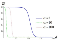
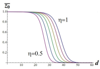
Figure 3: Bayesian posterior probability $\bar{z}_{0}\left(d\right)$ in coherent light interferometry with diffuse prior. Left: we show $\bar{z}_{0}(d)$ as a function of $d$ for different values of $\left|\alpha\right|$ and fixed quantum efficiency $\eta=0.7$. Right: $\bar{z}_{0}(d)$ as a function of $d$ for different values of $\eta$ and fixed photon number $\bar{n}=100$. Given the distance $t=({d-\bar{d}_{\frac{\pi}{2}}})/{\sigma_{d}}$ between the outcome and the expectation value the probability $\bar{z}_{0}\left(d\right)$ varies slowly with $\eta$.

The behavior of $\bar{z}_{0}\left(d\right)$ with respect to the number of photons injected and the quantum efficiency of the detectors is reported in Fig. 3. We note that the trend is the same for different $\bar{n}$ and $\eta$: the presence of non unit quantum efficiency in the detection process does not change the shape of $\bar{z}_{0}\left(d\right)$ and the same goes for the light intensity. In facts, the overall effect is to reduce the posterior probabilities, i. e. given an outcome $d$ and $\eta_{1}<\eta_{2}$ we have $\bar{z}_{0,1}\left(d\right)<\bar{z}_{0,2}\left(d\right)$, i.e. we get a lower value of $\bar{z}_{0}\left(d\right)$ when we lower down the efficiency of the apparatus.

That being said, for a given number of photons impinging on the device and efficiency of the photocounters, we can identify three different regions corresponding to different values of the outcome. In the range $0\leq d\leq 2\sigma_{d}$ the posterior probability is approximately $1$, in agreement with a sampling-theory approach. In this case the phase shift is so little that its origin is much more likely to be a random fluctuation rather than an actual perturbation. If $d\geq 4\sigma_{d}$ the posterior probability is approximately $0$: both the Bayesian and the Frequentist approach affirm that the phase shift has been induced by a perturbation. At last, $\bar{z}_{0}\left(d\right)$ falls from $1$ to $0$ as the value of the outcome increases within the interval $2\sigma_{d}\leq d\leq 4\sigma_{d}$. Since a frequentist analysis shall provide a value of $\bar{z}_{0}$ below $0.05$ we have that in this region we are in presence of the paradox.

On the other hand, one may find uneasy to say that an outcome four times $\sigma_{d}$ far from the mean value is to be associated to statistical fluctuations. In facts, we can describe what is happening for $2\sigma_{d}\leq d\leq 4\sigma_{d}$ as follows. Our measurement $d$ of the difference photocurrent gave a random value that was manifestly inconsistent with the expected value in absence of interaction; however, as a consequence of the prior assumed we are led to conclude that it would be even more improbable to observe that specific outcome were it the result of an interaction. That is, what makes the paradox arise is that the prior asks us to regard at every alternative possibility as an improbable coincidence. For this reason, in a real experiment an outcome in the range $2\sigma_{d}\leq d\leq 4\sigma_{d}$ should be interpreted as evidence of detection.

In approaching the most realistic description, we now discuss the occurrence of the paradox when a less diffuse prior is assumed. Here we consider a Gaussian-like distribution as a prior in order to account for our belief that a perturbation results in a small phase-shift around the expected value. In particular, we consider the so-called wrapped normal distribution, defined as follows:

$$g_{\sigma,\phi_{0}}\left(\phi\right)=\frac{1}{\sqrt{2\pi\sigma^{2}}}\sum_{k=-\infty}^{\infty}\exp\left[-\frac{\left(\phi-\phi_{0}+k\pi\right)^{2}}{2\sigma^{2}}\right],$$ (21)

The wrapped distribution is normalized on the interval $I$ and is characterized by two parameters, $\phi_{0}$ and $\sigma^{2}$, which correspond to the expectation value and variance of a normal distribution. In recalling that the mean value of the outcomes is $\bar{d}_{\frac{\pi}{2}}=0$ we impose $\phi_{0}=\frac{\pi}{2}$ but we let the variance of the prior free to vary in order to assess the relevance of our knowledge about the system with respect to the statistics. Note that since $\bar{z}_{0}$ is inversely proportional to the ratio $p\left(d|\phi\neq\phi_{0}\right)/p\left(d|\phi=\phi_{0}\right)$, which increases as the variance of the prior assumed for the alternative hypothesis decreases, we expect that the sharper is the the prior considered the higher will be the value of $\bar{z}_{0}$. For this reason we may expect the Lindley paradox not to occur when the variance $\sigma$ of $g_{\sigma,\phi_{0}}\left(\phi\right)$ is taken to be little with respect to the one of the Skellam distribution, given by Eq. (17). We report in Fig. 4 the results obtained substituting equation (16) with the proper expression for the prior (21), so that:

$$p\left(d|\phi\neq\phi_{0}\right)=\int_{I}d\phi\>p_{\phi}\left(d\right)g_{\sigma,\frac{\pi}{2}}\left(\phi\right).$$ (22)

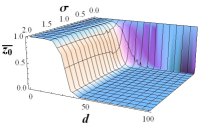
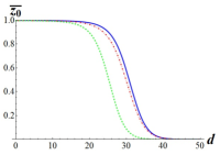
Figure 4: Posterior probability $\bar{z}_{0}$ in coherent light interferometry with wrapped normal prior. Left: $\bar{z}_{0}(d)$ as function of $d$ and $\sigma$ with $\eta=0.7$. The coherent amplitude is $\alpha=10$ so that $\bar{n}=100$ and $\sigma_{d}^{2}=70$. An actual disagreement with respect to a frequentist approach occurs for $0.2\leq\sigma\cap 2\sigma_{d}\leq d\leq 4\sigma_{d}$. Right: $\bar{z}_{0}(d)$ as a function of $d$. The continuous blue line and the dot-dashed red line are obtained for $\eta=0.7$ and $\sigma=1;\sigma=0,5$ respectively. The dashed green line refers to the case $\eta=0.5$ and $\sigma=0,5$.

At first, we see that if the variance of the prior is taken too small then the posterior probability does not evolve (with reference to the plotted range for d): we get $\bar{z}_{0}=z_{0}$ independently from the outcome $d$. From a mathematical perspective, this is due to the fact that the ratio $p\left(d|\phi=\phi_{0}\right)/p\left(d|\phi\neq\phi_{0}\right)$ appearing in the expression of $\bar{z}_{0}$ tends to unity as $p\left(d|\phi\neq\phi_{0}\right)$ tends to a delta $\delta\left(\phi-\phi_{0}\right)$. In facts, we are assuming a sharp prior centered in the mean value both for the null hypothesis and the alternative hypothesis. That is, we are somehow stating that $H_{0}$ and $H_{1}$ are equivalent as both of them, according to our prior models, lead to a measurement of $d$ to be associated to the outcome $d=\bar{d}_{\frac{\pi}{2}}$. Therefore, after a trial we cannot conclude anything else but that it is to be associated to a measurement of the mean value. Similarly, an evaluation of the posterior probability for the alternative hypothesis $p\left(d|\phi\neq\phi_{0}\right)$ yields $\overline{{1-z}_{0}}=1-z_{0}$. This last remark makes it clear that we are providing too much prior information and Bayesian inference can only confirm what we already know, without the possibility of improving our knowledge about the system. Conversely, if the prior distribution is diffuse, i. e. $\sigma>1$, we recover the case of flat prior examined above, where our knowledge is poor and, in turn, for $2\sigma_{d}\leq d\leq 4\sigma_{d}$ the paradox is again observed.

The most interesting region is $0.2\leq\sigma\leq 1$. A comparison between the values of $\bar{z}_{0}$ obtained employing a widespread prior and a sharper one, see the right panel of Fig. 4, shows that the latter distribution awards less probability to the null hypothesis, as we were expected to. However, the weight of the prior is not sufficient to avoid the paradox, which still occurs if $2\sigma_{d}\leq d\leq 4\sigma_{d}$ even for small values of the variance of the wrapped normal distribution. Fig. 4 also suggests that if the interferometer has poor detectors then the odds in favor of the alternative hypothesis will be lower. Nevertheless, in recalling that $\sigma_{d}$ decreases with $\eta$ it is possible to see that the net effect remains unchanged.

IV.2 Squeezed light interferometry

Let us now consider an input state of the form $\left|\psi\right\rangle=\left|\alpha\right\rangle\left|\lambda\right\rangle$, where $\alpha=\left|\alpha\right|e^{i\theta},\lambda=re^{i\varphi}\in\mathbb{C}$. That is, we replace the vacuum state $\left|0\right\rangle$ in mode $b$ with a squeezed-vacuum state $\left|\lambda\right\rangle$, containing $\bar{n}=\sinh^{2}(r)$ photons. The advantages gained by squeezing enhancement have been widely studied in literature. Here, our aim is to assess the convenience of employing squeezed light from a statistical perspective. That is, we address the possibility of getting by the Lindley paradox when the injected beam is previously squeezed.

Similarly to the previous case we will evaluate the posterior probability using a flat prior, at first, and then a peaked distribution. At the same time, we will pay attention to the contribution of the quantum efficiency. The difference with respect to the classical scheme seats in the distribution of the outcomes $p_{\alpha,\lambda,\phi}(d)$, which turns out to be difficult to be computed. However, since the expectation value $\bar{d}_{\phi}$ and the variance $\sigma_{d}^{2}$ may be calculated exactly we employ a Gaussian distribution for the outcomes as a first-order approximation:

$$p_{\alpha,\lambda,\phi}(d)=\frac{1}{\sqrt{2\pi\sigma_{d}^{2}}}\,e^{-[d-\eta\cos\phi(|\alpha|^{2}-\sinh^{2}r)]^{2}/2\sigma_{d}^{2}}\,,$$ (23)

where the variance is a function of the initial working point $\phi_{0}$ and of the measured phase shift $\phi$. Similarly to what happened in the previous case, $\sigma_{d}^{2}$ takes the minimum value at $\phi_{0}=\pi/2$, namely:

$$\sigma_{d}^{2}= \frac{1}{2}\eta\,(1-\eta)(|\alpha|^{2}+\sinh^{2}r)$$

$$+\eta^{2}\Bigg{\{}|\alpha|^{2}+2\sinh^{2}r\cosh^{2}r\cos^{2}\phi$$ (24)

$$+\sin^{2}\phi\left[\sinh^{2}r(1+2\alpha^{2})-2\alpha^{2}\sinh r\cosh r\right]\Bigg{\}}$$

whereas the expectation value results $\bar{d}_{\frac{\pi}{2}}=0$.

In order to test the consistency of an outcome $d=\bar{d}_{\frac{\pi}{2}}+t\cdot\sigma_{d}=t\cdot\sigma_{d}$ with the null hypothesis $H_{0}$ we pose $z_{0}=0.99$ and assume that the remainder probability $1-z_{0}$ is uniformly distributed over the interval $I=\left[0,\pi\right]$. Before computing the posterior probability we point out that the best sensitivity $\Delta\phi$ is achieved for $\varphi=\pi$ and $\left|\alpha\right|^{2}\gg\sinh^{2}\left(r\right)$. The posterior probability $\bar{z}_{0}$ that $\phi=\phi_{0}$ is, then, obtained by means of equation (10), with $\beta$ equal to $\phi$, leading to

$$p\left(d|\phi=\phi_{0}\right) =\int_{I}d\phi\>p_{\alpha,\lambda,\phi}\left(d\right)\delta\left(\phi-\phi_{0}\right)$$ (25)

$$p\left(d|\phi\neq\phi_{0}\right) =\int_{I}d\phi\>p_{\alpha,\lambda,\phi}\left(d\right).$$ (26)

The behavior obtained for $\bar{z}_{0}$ is very close to that observed for its classical counterpart, i.e. the dashed green line in Fig. 3. Indeed, we can identify a region where $\bar{z}_{0}$ tends to unity (for small values of $d$), a region where it is approximately zero (to the right) and a ”transition area”, where the posterior probability varies between these two limits. What matters most is that we are again in presence of the Lindley paradox: if we test the hypothesis concerning the detection of a perturbation by means of the Bayes’ theorem we will end up in a misleading analysis. It is possible to see from the plot of Fig. 5 that the situation does not change in presence of non ideal photodetectors. In the same vein, when we consider input states containing a higher number of photons and such that the optimal conditions mentioned above are still satisfied (i. e. $\varphi=\pi$ and $\left|\alpha\right|^{2}\gg\sinh^{2}r$), the posterior probability approaches zero for lower values of $d/\sigma_{d}$. However, the contribution gained from the use of higher intensity light is not sufficient to make it disappear.

At last, we take into account the most actual case with squeezed input light and a Gaussian-like prior distribution wherein the statistical description. The change in the shape of $p\left(d|\phi\neq\phi_{0}\right)$ has the usual effect of decreasing the value of $\bar{z}_{0}$, as it is illustrated in Fig. 5. Nevertheless, we have to say that neither in this conditions we can have a consistent Bayesian statistical inference. That is, the value of the posterior probability does not decrease, not even taking an appreciably peaked prior, until the outcome is more than several $\sigma_{d}$ far from the expectation value.

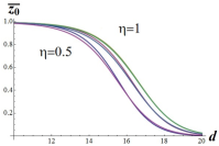
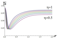
Figure 5: Bayesian posterior probability $\bar{z}_{0}(d)$ in squeezed light interferometry. Left: $\bar{z}_{0}(d)$ as a function of $d$ for efficiency $\eta$ from $0.5$ to $1.0$ and for $\alpha=10$, $r=1$, $\varphi=\pi$. Right: the posterior probability for given distance $|d-\bar{d}_{\phi}|=3\sigma_{d}$ and the same values of the state parameters (while $\phi_{0}=\pi/2,\phi=0$ in $\sigma_{d}$).

V Conclusions

We have addressed the occurrence of the so-called Lindley paradox in the analysis of data coming from homodyne detection and optical interferometry. We found that the Lindley paradox may indeed occur. In particular, we have shown that the Bayesian approach is somehow misleading if a scarce information about the prior distributions is available, as it happens in the evaluation of the effect of an external perturbation, and sampling-theory should be preferred. Concerning MZ interferometers, we have shown that Lindley paradox appears both for coherent and squeezed signals and is present for any value of the quantum efficiency of the involved detectors. On the other hand, the disagreement between Bayesian and frequentist approach is less pronounced for increasing noise and may be softened by using a suitable, more localized, priors.

Our results, besides being of fundamental interest for interferometry, are of practical significance for quantum state reconstruction, where calibration of homodyne detectors represents a crucial step for the implementation of quantum tomography reh04 .

Appendix A Posterior probabilities

Consider a physical system where the quantity $X$ may be measured and assume that the outcomes from the measurement of $X$ are distributed according to a normal distribution with an unknown mean value $\phi$ and a known variance $\sigma^{2}$. We perform a measurement of $X$ and on the basis of the outcome $x$ we want to test which of the two following hypothesis is true

$$H_{0}:\hbox{the mean value is equal to a given value}\,\,\phi=\phi_{0}$$ (27)

$$H_{1}:\hbox{the mean value is not the value above}\,\,\phi\neq\phi_{0}\,.$$ (28)

We assume to have some prior knowledge on the system, which may be expressed in form of some a priori probabilities $p(H_{0})$ and $p(H_{1})=1-p(H_{0})$ for the two hypothesis. The measurement of $X$ is, in turn, intended to upgrade our knowledge of the system. Given the result $x$, Bayes theorem says that

$$p(H_{k}|x)p(x)=p(x|H_{k})p(H_{k})\,,$$

for $k=0,1$, where $p(H_{k})$ is the a priori probability introduced above, $p(x|H_{k})$ is the conditional distribution of the outcomes given a hypothesis, $p(x)=p(x|H_{0})p(H_{0})+p(x|H_{1})p(H_{1})$ is the overall distribution of the outcomes, independently which hypothesis is actually true, and $p(H_{k}|x)$ is the a posteriori probability of the hypothesis $H_{k}$, i.e. the quantity of interest here. Using the Bayes theorem we may evaluate the a posteriori probabilities, e.g. $p(H_{0}|x)$ is given by

$$p(H_{0}|x) =\frac{p(x|H_{0})p(H_{0})}{p(x)}$$

$$=\frac{p(x|H_{0})p(H_{0})}{p(x|H_{0})p(H_{0})+p(x|H_{1})p(H_{1})}$$

$$=\left[1+\frac{p(x|H_{1})p(H_{1})}{p(x|H_{0})p(H_{0})}\right]^{-1}$$

$$=\left[1+\frac{1-p(H_{0})}{p(H_{0})}\frac{p(x|H_{1})}{p(x|H_{0})}\right]^{-1}\,,$$ (29)

which, upon the substitutions $p(H_{0})\rightarrow z_{0}$ and $p(H_{0}|x)\rightarrow\bar{z}_{0}$, coincides with Eq. (1).

Now, in order to evaluate explicitly the posterior distribution we assign some prior distribution $\pi_{k}(\phi)\equiv p(\phi|H_{k})$ to the mean value under the two hypothesis. According to (27) and (28) we write

$$\pi_{0}(\phi)=\delta(\phi-\phi_{0})\,$$

and assign the rest of the prior probability as a normal distribution with variance $\tau$, i.e.

$$\pi_{1}(\phi)=(2\pi\tau^{2})^{-1/2}\exp\{-(\phi-\phi_{0})^{2}/2\tau^{2}\}\,.$$

It is now straightforward to evaluate the conditional probabilities as

$$p(x|H_{k})=\int\!d\phi\,\pi_{k}(\phi)\,p(x|\phi)\,,$$

which leads to

$$p(x|H_{0}) =(2\pi\sigma^{2})^{-1/2}\,e^{-(\phi-\phi_{0})^{2}/2\sigma^{2}}$$ (30)

$$p(x|H_{1}) =[2\pi(\sigma^{2}+\tau^{2})]^{-1/2}\,e^{-(\phi-\phi_{0})^{2}/2(\sigma^{2}+\tau^{2})}\,.$$ (31)

Overall, Eq. (29) rewrites as

$$p(H_{0}|x)=\Bigg{[}1+ \frac{1-p(H_{0})}{p(H_{0})}\sqrt{\frac{\sigma^{2}}{\sigma^{2}+\tau^{2}}}$$

$$\times \exp\left(\frac{\tau^{2}}{2\sigma^{2}}\frac{(x-\phi_{0})^{2}}{\sigma^{2}+\tau^{2}}\right)\Bigg{]}^{-1}\,.$$ (32)

Upon substituting $\phi_{0}=0$ and $\sigma=1$ we arrive at Eq. (2).

References

- (1) K. S. Thorne, Rev. Mod. Phys. 52, 285 (1980).
- (2) R. X. Adhikari, Rev. Mod. Phys. 86, 121 (2014).
- (3) V. B. Braginsky, Astron. Lett. 34, 558 (2008).
- (4) V. B. Braginsky, F. Ya. Khalili, F. Ya., Quantum Measurement (Cambridge University Press, Cambridge, 1992).
- (5) C. M. Caves, Phys. Rev. D 23, 1693 (1981).
- (6) R. S. Bondurant and J. H. Shapiro, Phys. Rev. A 30, 2548 (1984).
- (7) B. Yurke, S. L. McCall and J. R. Klauder, Phys. Rev. A 33, 4033 (1986).
- (8) M. J. Holland and K. Burnett, Phys. Rev. Lett. 71, 1355 (1993).
- (9) F. W. Sun, B. H. Liu, Y. X. Gong, Y. F. Huang, Z.Y. Ou, G. C. Guo, EPL 82, 24001 (2008).
- (10) M. G. A. Paris, Phys. Lett. A 201, 132 (1995).
- (11) The LIGO Scientific Collaboration, Nature Phot. 7, 613 (2013).
- (12) A. A. Berni,T. Gehring, B. M. Nielsen, V. Handchen, M. G. A. Paris, U.L. Andersen, Nature Phot. 9, 577 (2015).
- (13) M. G. A. Paris, Phys. Lett. A 225, 23 (1997).
- (14) L. Pezzé, A. Smerzi, G. Khoury, J. F. Hodelin, and D. Bouwmeester, Phys. Rev. Lett. 99, 223602 (2007).
- (15) L. Pezzé, A. Smerzi, Phys. Rev. Lett. 100, 073601 (2008).
- (16) S. Olivares, M. G. A. Paris, J. Phys. B 42, 055506 (2009)
- (17) B. Teklu, S Olivares, M. G. A. Paris, J. Phys. B 42, 035502 (2009).
- (18) M. G. Genoni, S. Olivares, M. G. A. Paris, Phys. Rev. Lett. 106, 153603 (2011).
- (19) M. G. Genoni, S. Olivares, D. Brivio, S. Cialdi, D. Cipriani, A. Santamato, S. Vezzoli, M. G. A. Paris, Phys. Rev. A 85, 043817 (2012).
- (20) S. Olivares, S. Cialdi, F. Castelli, M. G. A. Paris, Phys. Rev. A 87, 050303(R) (2013).
- (21) H. Jeffrey, Theory of probability (Oxford Univ. Press, 1948).
- (22) D. V. Lindley, Biometrika 44, 187 (1957).
- (23) Z. Hradil, R. Myska, J. Perina, M. Zawisky, Y. Hasegawa, and H. Rauch Phys. Rev. Lett. 76, 4295 (1996).
- (24) J. P. Dowling, Phys. Rev. A 57, 4736 (1998).
- (25) G. M. D’Ariano, M. G. A. Paris, R. Seno, Phys. Rev. A 54, 4495 (1996).
- (26) D. V. Lindley, Biometrika 64, 207 (1977).
- (27) G. Shafer, J. Am. Stat. Ass. 77, 325 (1982).
- (28) H. M. Wiseman, D. W. Berry, S. D. Bartlett, B. L. Higgins, G. J. Pryde, IEEE J. Sel. Top. Quantum Electron. 15, 1661 (2009).
- (29) A. Kumar De, D. Roy, D. Goswami, Phys. Rev. A 83, 015402 (2011).
- (30) T. Reisinger, G. Bracco, B. Holst, New. J. Phys. 13, 065016 (2011).
- (31) B. T. Kirby and J. D. Franson, Phys. Rev. A 89, 033861 (2014).
- (32) X. M. Feng, G. R. Jin, W. Yang, Phys. Rev. A 90, 013807 (2014).
- (33) M. G. A. Paris and J. Rehacek (Eds.) Quantum state estimation, Lect. Notes Phys. 649, (Springer, Berlin, 2004).
- (34) J. G. Skellam, J. Roy. Stat. Soc. 109, 296 (1946).