LAPTH-058/15 Chern-Simons dilaton black holes in 2+1 dimensions

We construct rotating magnetic solutions to the three-dimensional Einstein-Maxwell-Chern-Simons-dilaton theory with a Liouville potential. These include a class of black hole solutions which generalize the warped AdS black holes. The regular black holes belong to two disjoint sectors. The first sector includes black holes which have a positive mass and are co-rotating, while the black holes of the second sector have a negative mass and are counter-rotating. We also show that a particular, non-black hole, subfamily of our three-dimensional solutions may be uplifted to new regular non-asymptotically flat solutions of five-dimensional Einstein-Maxwell-Chern-Simons theory.

1 Introduction

Lower dimensional gravity provides an arena for constructing exact analytical black hole solutions in a wide variety of gravitating field theories. Most of the known black hole solutions are static. The celebrated BTZ black hole in $2+1$ dimensions [2] can be either static or rotating, but the rotating solutions can be transformed to the static one by a local coordinate transformation. The first intrisincally rotating black holes, now known as warped AdS₃ black holes [3], were constructed as solutions to topologically massive gravity [4] in [5], and then generalized to solutions of cosmological topologically massive gravity in [6], of topologically massive gravitoelectrodynamics (TMGE) [7] in [8], of new massive gravity [9] in [10], of $R^{3}$ extended new massive gravity [11] in [12], and of generalized massive gravity [9] in [13].

In this paper, we shall extend the warped AdS black hole class to a more general class of intrinsincally rotating black holes. The warped AdS black holes of [8] were solutions of three-dimensional Einstein-Maxwell theory augmented by both gravitational and electromagnetic Chern-Simons terms [7], which reduces to Einstein-Maxwell-Chern-Simons theory when the gravitational Chern-Simons term is absent. In [14], a class of rotating electric solutions to the cosmological Einstein-Maxwell-Chern-Simons-dilaton theory were obtained for a special relation between the model parameters. From these solutions, a class of rotating magnetic solutions to the same theory were generated in [15]. Considering this theory, we discuss in the next section the reduction of the field equations along the lines followed in [8]. We then show in Sect. 3 that a simple ansatz generalizing that of [8] leads to rotating magnetic solutions more general than those of [15]. The global structure of these solutions is analyzed in Sect. 4, where a subclass of regular black hole solutions is found in a certain parameter range. The mass, angular momentum and other observables of these black holes are computed in Sect. 5. In Sect. 6 we show that another subclass of our solutions may be uplifted to new regular non-asymptotically flat solutions of five-dimensional Einstein-Maxwell-Chern-Simons theory. Our results are summarized in the final section.

2 Reduction of the field equations

Self-gravitating dilatonic topologically massive electrodynamics is defined by [14]

$$I_{E} = \int d^{3}x\sqrt{|g|}\left[\frac{1}{2\kappa}R-2g^{\mu\nu}\partial_{\mu}\phi\partial_{\nu}\phi-\frac{\Lambda}{\kappa}e^{b\phi}-\frac{1}{4}e^{c\phi}g^{\mu\nu}g^{\rho\sigma}F_{\mu\rho}F_{\nu\sigma}\right]$$ (2.1)

$$+\frac{\mu}{2}\int d^{3}x\epsilon^{\mu\nu\rho}A_{\mu}\partial_{\nu}A_{\rho}\,,$$

with $\kappa=8\pi G$ the Einstein gravitational constant (which in $2+1$ dimensions can be either positive or negative), $b$ and $c$ the coupling constants of the dilatonic field $\phi$ to the cosmological constant $\Lambda$ and to the Maxwell field $F=dA$, and $\mu$ the Chern-Simons coupling constant ($\epsilon^{\mu\nu\rho}$ is the antisymmetric symbol).

Assuming the existence of two commuting Killing vectors, we choose the parametrisation [16, 7]

$$ds^{2} = \lambda_{ab}\left(\rho\right)dx^{a}dx^{b}+\zeta^{-2}\left(\rho\right)R^{-2}\left(\rho\right)d\rho^{2}\quad(a,b=0,1),$$

$$A = \psi_{a}\left(\rho\right)dx^{a}$$ (2.2)

($x^{0}=t,$ $x^{1}=\varphi$), where $\lambda$ is the $2\times 2$ matrix

$$\lambda=\left(\begin{array}[]{cc}T+X&Y\\ Y&T-X\end{array}\right)\,,$$ (2.3)

$R^{2}\equiv\mathbf{X}^{2}$ is the Minkowski pseudo-norm of the vector $\mathbf{X}\left(\rho\right)=\left(T,X,Y\right)$

$$\mathbf{X}^{2}=\eta_{ij}X^{i}X^{j}=-T^{2}+X^{2}+Y^{2}\,,$$ (2.4)

and $\zeta$ a scale factor. The stationary sector of the spacetime of metric (2.2) corresponds to the spacelike sector $R^{2}>0$ of (2.4), with the same signature $(-++)$.

This parametrisation reduces the action (2.1) to the form

$$I=\int d^{2}x\int d\rho\,L$$ (2.5)

where $L$ is the effective Lagrangian

$$L=\frac{1}{2}\left[\frac{\zeta}{2\kappa}\mathbf{X}^{\prime 2}-4\zeta R^{2}\phi^{\prime 2}-\frac{2\Lambda}{\kappa\zeta}e^{b\phi}+\zeta e^{c\phi}\overline{\psi}^{\prime}\left(\mathbf{\Sigma}.\mathbf{X}\right)\psi^{\prime}+\mu\overline{\psi}\psi^{\prime}\right]\,,$$ (2.6)

where ${}^{\prime}=\partial/\partial\rho$, the ”Dirac” matrices $\Sigma^{i}$ are defined by

$$\Sigma^{0}=\left(\begin{array}[]{cc}0&1\\ -1&0\end{array}\right)\ ,\ \Sigma^{1}=\left(\begin{array}[]{cc}0&-1\\ -1&0\end{array}\right)\ ,\ \Sigma^{2}=\left(\begin{array}[]{cc}1&0\\ 0&-1\end{array}\right)\,,$$ (2.7)

and $\overline{\psi}\equiv\psi^{T}\Sigma^{0}$ is the Dirac adjoint of the ”spinor” $\psi$. In passing from (2.1) to (2.6), we have set the sign convention for the antisymmetric symbol to $\epsilon^{012}=-1$ (corresponding to $\epsilon_{012}=+1$).

Variation of the Lagrangian $L$ with respect to $\psi$ gives the equation

$$\partial_{\rho}\left[\mu\psi-\zeta e^{c\phi}\left(\mathbf{\Sigma.X}\right)\psi^{\prime}\right]=0\,,$$ (2.8)

which is integrated, up to a gauge transformation, by

$$\zeta\psi^{\prime}=\frac{\mu}{R^{2}}e^{-c\phi}(\mathbf{\Sigma.X})\psi\,.$$ (2.9)

Defining the wedge product of two vectors $\mathbf{X}$ and $\mathbf{Y}$ by

$$\left(\mathbf{X\wedge Y}\right)^{i}=\eta^{ij}\epsilon_{jkl}X^{k}Y^{l}$$ (2.10)

with $\epsilon_{012}=+1$, the spinor equation (2.9) can be shown [7] to be equivalent to the vector dynamical equation

$$\zeta\mathbf{S}^{\prime}=\frac{2\mu}{R^{2}}e^{-c\phi}\mathbf{X}\wedge\mathbf{S}$$ (2.11)

for the “spin” vector

$$\mathbf{S}=-\frac{\kappa}{2}\overline{\psi}\mathbf{\Sigma}\psi$$ (2.12)

of components

$$S^{0}=\frac{\kappa}{2}\left[\psi_{0}^{2}+\psi_{1}^{2}\right]\,,\quad S^{1}=\frac{\kappa}{2}\left[\psi_{0}^{2}-\psi_{1}^{2}\right]\,,\quad S^{2}=\kappa\psi_{0}\psi_{1}\,.$$ (2.13)

Note that our trading of a spinor equation (2.9) for a vector equation (2.11) is possible only because the spin vector is null,

$$\mathbf{S}^{2}=0.$$ (2.14)

Next, vary $L$ with respect to $\mathbf{X}$, leading to the equation

$$\mathbf{V}\equiv\mathbf{X}^{\prime\prime}+8\kappa\mathbf{X}\phi^{\prime 2}=\kappa e^{c\phi}\overline{\psi}^{\prime}\mathbf{\Sigma}\psi^{\prime}=\frac{2\mu^{2}}{\zeta^{2}R^{2}}e^{-c\phi}\left[\frac{2}{R^{2}}\left(\mathbf{S}.\mathbf{X}\right)\mathbf{X}-\mathbf{S}\right]\,,$$ (2.15)

where we have used Eq. (2.9) and the definition (2.12). Similarly, variation of $L$ with respect to $\phi$ leads to

$$\left(R^{2}\phi^{\prime}\right)^{\prime}=\frac{b\Lambda}{4\kappa\zeta^{2}}e^{b\phi}-\frac{c\mu^{2}}{4\kappa\zeta^{2}R^{2}}e^{-c\phi}\left(\mathbf{S}.\mathbf{X}\right)\,.$$ (2.16)

Finally, variation of the Lagrangian with respect to the Lagrange multiplier $\zeta$ leads to the Hamiltonian constraint

$$H\equiv\frac{1}{4\kappa}\left[\mathbf{X}^{\prime 2}-8\kappa R^{2}\phi^{\prime 2}+\frac{4\Lambda}{\zeta^{2}}e^{b\phi}+\frac{4\mu^{2}}{\zeta^{2}R^{2}}e^{-c\phi}\left(\mathbf{S}.\mathbf{X}\right)\right]=0\,.$$ (2.17)

Equations (2.16) and (2.17) involve the scalar $\mathbf{S}.\mathbf{X}$ which can be evaluated by taking the scalar product of Eq. (2.15) with $\mathbf{X}$ as

$$\left(\mathbf{S}.\mathbf{X}\right)=\frac{R^{2}\zeta^{2}}{2\mu^{2}}e^{c\phi}\left(\mathbf{X.X}^{{}^{\prime\prime}}+8\kappa R^{2}\phi^{\prime 2}\right)\,.$$ (2.18)

Inserting this in Eqs. (2.16) and (2.17) we obtain the simplified equations

$$\left(R^{2}\phi^{\prime}\right)^{\prime}+\frac{c}{8\kappa}\left(\mathbf{X.X}^{{}^{\prime\prime}}+8\kappa R^{2}\phi^{\prime 2}\right)-\frac{b\Lambda}{4\kappa\zeta^{2}}e^{b\phi}=0$$ (2.19)

and

$$\mathbf{X}^{\prime 2}+2\mathbf{X.X}^{{}^{\prime\prime}}+8\kappa R^{2}\phi^{\prime 2}+\frac{4\Lambda}{\zeta^{2}}e^{b\phi}=0\,.$$ (2.20)

These last two equations may be combined to yield

$$\left(R^{2}\phi^{\prime}-\frac{c}{8\kappa}\left(\mathbf{X.X}^{\prime}\right)\right)^{\prime}=\frac{\Lambda}{2\kappa\zeta^{2}}\left(c+\frac{b}{2}\right)e^{b\phi}\,.$$ (2.21)

This last equation can be easily integrated only if the dilaton coupling constants are related by

$$b+2c=0\,,$$

which we assume henceforth. This integration leads to

$$R^{2}\phi^{\prime}=\frac{c}{8\kappa}\left(RR^{\prime}+d\right)\,,$$ (2.22)

where $d$ is an integration constant.

Finally, the independent reduced field equations can be taken to be (2.22), (2.20) and (2.11) (where the spin vector $\mathbf{S}$ is given in terms of $\mathbf{X}$ and $\phi$ by (2.15)), supplemented by the conditions, following from (2.14) and (2.13), that the vector $\kappa^{-1}\mathbf{S}$ is future null,

$$\mathbf{S}^{2}=0\,,\quad\kappa^{-1}S^{0}>0\,.$$ (2.23)

3 Black Hole Solutions

3.1 Power-law ansatz

Black hole solutions were found in TMGE by making the ansatz [8]

$$\mathbf{X}=\boldsymbol{\alpha}\rho^{2}+\boldsymbol{\beta}\rho+\boldsymbol{\gamma}\,,$$ (3.1)

where $\boldsymbol{\alpha}$, $\boldsymbol{\beta}$ and $\boldsymbol{\gamma}$ are three linearly independent constant vectors, and the vector $\boldsymbol{\alpha}$ is null and orthogonal to the vector $\boldsymbol{\beta}$,

$$\boldsymbol{\alpha}^{2}=0\,,\quad\boldsymbol{\alpha}.\boldsymbol{\beta}=0\,.$$ (3.2)

In the present dilatonic context, we shall generalize this ansatz by assuming

$$\mathbf{X}=\boldsymbol{\alpha}\rho^{q+p}+\boldsymbol{\beta}\rho^{q}+\boldsymbol{\gamma}\rho^{q-p}\,,$$ (3.3)

where $q$ and $p\neq 0$ are real numbers (the ansatz (3.3) degenerates for $p=0$) which should reduce to $q=p=1$ in the limit $c=0$ of vanishing dilaton coupling, and the constant vectors $\boldsymbol{\alpha}$, $\boldsymbol{\beta}$ and $\boldsymbol{\gamma}$ are again constrained by (3.2). It follows from these assumptions that

$$R^{2}=m\rho^{2q}+n\rho^{2q-p}+l\rho^{2q-2p}\,,$$ (3.4)

with

$$m=2\boldsymbol{\alpha}.\boldsymbol{\gamma}+\boldsymbol{\beta}^{2}\,,\quad n=2\boldsymbol{\beta}.\boldsymbol{\gamma}\,,\quad l=\boldsymbol{\gamma}^{2}\,.$$ (3.5)

Inserting the functional form (3.4) of $R^{2}(\rho)$ into (2.22), we obtain

$$\phi^{\prime}=\frac{c}{16\kappa}\frac{2qm\rho^{2q-1}+(2q-p)n\rho^{2q-p-1}+(2q-2p)l\rho^{2q-2p-1}+2d}{m\rho^{2q}+n\rho^{2q-p}+l\rho^{2q-2p}}\,.$$ (3.6)

This can be easily integrated to $\phi\propto\ln\rho$ if 1) the constant $2d$ can be grouped with one of the three monomials in the numerator, implying either $2q-1=0$, $2q-p-1=0$, or $2q-2p-1=0$, only the second possibility

$$p=2q-1$$ (3.7)

being consistent with the constraint that $p$ and $q$ reduce to $1$ in the limit of vanishing dilaton coupling; 2) the coefficients in the numerator are matched to those in the denominator so that $\phi^{\prime}\propto\rho^{-1}$:

$$n+2d=2qn\,,\quad 2(1-q)l=2ql\,.$$ (3.8)

(where we have replaced $p$ in terms of $q$ according to (3.7)). The first relation fixes the integration constant $d$ for the dilaton field equation (2.19) in terms of the metric parameters. The second relation is solved either by $q=1/2$, leading to $p=0$, which we have excluded, or by $l=0$. We are thus led to add to the ansatz (3.3), (3.2) the complementary assumption

$$\boldsymbol{\gamma}^{2}=0\,,$$ (3.9)

leading to the solution of (3.6)

$$\phi=\frac{cq}{8\kappa}\,\ln\left(\frac{\rho}{\rho_{1}}\right)\,,$$ (3.10)

with $\rho_{1}>0$ a new integration constant.

Next, fixing without loss of generality the scale parameter $\zeta$ to

$$\zeta=\mu\,,$$ (3.11)

we compute the left-hand side of Eq. (2.15):

$$\mathbf{V}=\left[(3q-1)(3q-2)+\frac{c^{2}q^{2}}{8\kappa}\right]\boldsymbol{\alpha}\rho^{3q-3}+\left[q(q-1)+\frac{c^{2}q^{2}}{8\kappa}\right]\left(\boldsymbol{\beta}\rho^{q-2}+\boldsymbol{\gamma}\rho^{-q-1}\right)\,.$$ (3.12)

Squaring the right-hand side of Eq. (2.15), we find that this vector must be null, as the spin vector $\mathbf{S}$ (Eq. (2.14)). This is ensured if $\mathbf{V}$ is collinear with $\boldsymbol{\alpha}$, which is possible only if

$$q=\frac{1}{1+c^{2}/8\kappa}$$ (3.13)

(the other possibility $q=0$ does not lead to a consistent solution). It follows that $c^{2}q/8\kappa=1-q$, so that

$$e^{c\phi}=\left(\frac{\rho}{\rho_{1}}\right)^{1-q}\,,\quad\mathbf{V}=2(1-2q)^{2}\boldsymbol{\alpha}\,\rho^{3q-3}\,.$$ (3.14)

Computing the spin vector from the inverse of (2.15),

$$\mathbf{S}=\frac{1}{2}\,e^{c\phi}\left[2(\mathbf{V}.\mathbf{X})\mathbf{X}-R^{2}\mathbf{V}\right]\,,$$ (3.15)

we obtain

$$\mathbf{S} = (1-2q)^{2}\rho_{1}^{q-1}\left[2(\boldsymbol{\alpha}.\boldsymbol{\gamma})\mathbf{X}\rho^{q-1}-R^{2}\boldsymbol{\alpha}\rho^{2q-2}\right]$$ (3.16)

$$= (1-2q)^{2}\rho_{1}^{q-1}\left[k\boldsymbol{\alpha}\wedge\boldsymbol{\beta}\,\rho^{4q-2}+2k\boldsymbol{\alpha}\wedge\boldsymbol{\gamma}\,\rho^{2q-1}+2(\boldsymbol{\alpha}.\boldsymbol{\gamma})\boldsymbol{\gamma}\right]\,.$$

To obtain the second form of $\mathbf{S}$, we have used (3.4), and the vector relations, which follow from (3.2)

$$\boldsymbol{\alpha}\wedge\boldsymbol{\beta}=-k\boldsymbol{\alpha}\,,\quad\boldsymbol{\beta}^{2}=k^{2}\,,$$ (3.17)

where $k$ is some constant. We then see that the dynamical equation (2.11) is satisfied provided

$$k=\frac{\rho_{1}^{1-q}}{2q-1}\,.$$ (3.18)

Finally, the Hamiltonian constraint in the form (2.20) is also satisfied provided

$$\boldsymbol{\alpha}.\boldsymbol{\gamma}=\frac{q+4(2q-1)\Lambda/\mu^{2}}{2(1-3q)}\,k^{2}\,,$$ (3.19)

for $q\neq 1/3$. For $q=1/3$ ($c^{2}=16\kappa$) and $\Lambda=\mu^{2}/4$, the value of the scalar product $\boldsymbol{\alpha}.\boldsymbol{\gamma}$ remains arbitrary.

We choose for the basis vectors $\boldsymbol{\alpha}$, $\boldsymbol{\beta}$ and $\boldsymbol{\gamma}$ the parametrisation, which generalizes that made in [8],

$$\boldsymbol{\alpha}=k^{3}\left(\epsilon/2,-\epsilon/2,0\right)\,,\quad\boldsymbol{\beta}=k\left(\omega,-\omega,-1\right)\,,\quad\boldsymbol{\gamma}=k^{-1}\left(z+u,z-u,v\right)$$ (3.20)

($\epsilon^{2}=1$). These automatically satisfy (3.2) and (3.17), while the constraint (3.9) implies the relation

$$u=v^{2}/4z\,.$$ (3.21)

The value of the parameter $z$ may be computed from $\boldsymbol{\alpha}.\boldsymbol{\gamma}=-\epsilon k^{2}z$, where the scalar product $\boldsymbol{\alpha}.\boldsymbol{\gamma}$ is given by (3.19). The scalar function $R^{2}$ is, from (3.4),

$$R^{2}=k^{2}\beta^{2}\rho\left(\rho^{2q-1}-\rho_{0}^{2q-1}\right)\,,$$ (3.22)

where the parameters $\beta^{2}$ (real) and $\rho_{0}^{2q-1}$ ($\rho_{0}>0$) are defined by

$$k^{2}\beta^{2} = k^{2}(1-2\epsilon z)=\boldsymbol{\beta}^{2}+2\boldsymbol{\alpha}.\boldsymbol{\gamma}\,,$$

$$k^{2}\beta^{2}\rho_{0}^{2q-1} = 2(v+2\omega z)=-2\boldsymbol{\beta}.\boldsymbol{\gamma}\,,$$ (3.23)

leading to

$$\omega=\frac{\epsilon}{2(1-\beta^{2})}\left(k^{2}\beta^{2}\rho_{0}^{2q-1}-2v\right)\,.$$ (3.24)

The resulting metric may be written in terms of the three parameters $k$, $\rho_{0}$ and $v$ as

$$ds^{2} = \frac{\epsilon(1-\beta^{2})}{k}\,\rho^{1-q}\left[dt-\frac{\epsilon(k^{2}\rho^{2q-1}-v)}{1-\beta^{2}}d\varphi\right]^{2}$$ (3.25)

$$-\frac{\epsilon k^{3}\beta^{2}\rho^{q}(\rho^{2q-1}-\rho_{0}^{2q-1})}{1-\beta^{2}}d\varphi^{2}+\frac{d\rho^{2}}{k^{2}\mu^{2}\beta^{2}\rho\left[\rho^{2q-1}-\rho_{0}^{2q-1}\right]}\,,$$

with $\beta^{2}$ a real parameter given in terms of the model parameters by

$$\beta^{2}=\frac{1-2q}{1-3q}\left(1-\frac{4\Lambda}{\mu^{2}}\right)\,,$$ (3.26)

when $q\neq 1/3$, $\beta^{2}$ remaining arbitrary when $q=1/3$ with $\Lambda=\mu^{2}/4$. Solving Eq. (2.13) for $\psi$, we obtain the electromagnetic field generating this gravitational field:

$$A=\pm\sqrt{\frac{\epsilon(1-2q)}{\kappa}}\left[\epsilon(1-\beta^{2})dt-(k^{2}\rho^{2q-1}-v)d\varphi\right]\,.$$ (3.27)

The constant electric potential is irrelevant and may be gauged away, the magnetic potential $A_{\varphi}$ leading both to a magnetic field and to an electric field $F^{t\rho}$ because the metric (3.25) is non-diagonal. This electromagnetic field is real provided

$$\epsilon={\rm sign}[\kappa(1-2q)]\,.$$ (3.28)

For $q=1$ ($c=0$), the solution (3.25), (3.27) reduces to the non-dilatonic solution obtained in [8] for $\lambda=0$ (no gravitational Chern-Simons term). Note however that the black holes of [8] are regular for $0<\beta^{2}<1$, while as we shall see in the next section the present dilatonic solution can correspond to regular black holes only if $\beta^{2}<0$.

The form of the metric (3.25) breaks down for $\beta^{2}=1$ and $\beta^{2}=0$. For $\beta^{2}=1$ ($\Lambda=(q/(1-2q))\mu^{2}/4$), $z=0$ implying $v=0$ from (3.21), so also $\rho_{0}=0$. The metric, depending on the two independent parameters $\omega$ and $u$, may be written in the ADM form (4.1) with $v^{2}/(1-\beta^{2})$ replaced with $2\epsilon u$. For $\beta^{2}=0$ ($\Lambda=\mu^{2}/4$ with $q\neq 1/3$), the metric is obtained from (3.25) by replacing $-k^{2}\beta^{2}\rho_{0}^{2q-1}$ with $2\nu\equiv-2(v+\epsilon\omega)\neq 0$.

To conclude this part, we comment on the relation of our magnetic power-law solution with that of Castelo Ferreira [15] (similar comments can be made concerning the electric solution of [14]). The space-metric metric of [15] is parametrized by

$$ds^{2}=-f^{2}(dt+A\,d\varphi)^{2}+dr^{2}+h^{2}\,d\varphi^{2}\,,$$ (3.29)

with $f^{2}\propto r$, $h^{2}\propto r^{2p_{CF}-1}$, $p_{CF}=4\kappa/c^{2}$. This metric can be transformed to the form (2.2) by the radial coordinate transformation $d\rho=\mu Rdr$, with $R^{2}=f^{2}h^{2}\propto r^{2p_{CF}}$, leading to $\rho\propto r^{p_{CF}+1}$. The resulting vector $\mathbf{X}(\rho)$ is of the form (3.3) with $p=(p_{CF}-1)/(p_{CF}+1)$ and $q=p_{CF}/(p_{CF}+1)$, different from our exponents (3.7) and (3.13), the basis vectors $\boldsymbol{\alpha}$, $\boldsymbol{\beta}$ and $\boldsymbol{\gamma}$ obeying the constraints (3.2) and (3.9), together with the additional constraint

$$\boldsymbol{\beta}.\boldsymbol{\gamma}=0\,,$$ (3.30)

accounting for the fact that $R^{2}\propto\rho^{2q}$ is a monomial. The price to pay for this additional constraint is that the Hamiltonian constraint (2.17) can only be satisfied if there is a specific relation between the dimensionless coupling constants $c^{2}/\kappa$ and $\Lambda/\mu^{2}$, Eq. (3.6) of [15].

3.2 Case $c^{2}=8\kappa$

For $c^{2}=8\kappa$, (3.13) leads to $q=1/2$, corresponding to $p=0$ from (3.7), so that the power-law ansatz (3.3) is degenerate. In this case, we replace this ansatz by the logarithmic ansatz

$$\mathbf{X}=\boldsymbol{\alpha}\rho^{1/2}\ln(\rho/\rho_{0})+\boldsymbol{\beta}\rho^{1/2}\,,$$ (3.31)

with only two linearly independant constant vectors $\boldsymbol{\alpha}$ and $\boldsymbol{\beta}$ obeying the constraints (3.2). This leads to $R^{2}=m\rho$, so that from (2.22),

$$\phi^{\prime}=\frac{m+2d}{2cm\rho}\,.$$ (3.32)

The computation of $\mathbf{V}$ then leads to

$$\mathbf{V}=\frac{d(m+d)}{m^{2}}\,\rho^{-2}\mathbf{X}\,,$$ (3.33)

which is null, $\mathbf{V}^{2}=0$, only if $d(m+d)=0$, leading to

$$\phi^{\prime}=\pm\frac{1}{2c\rho}\,,\quad\mathbf{V}=0\,,$$ (3.34)

implying also $\mathbf{S}=0$, which in turn means $\psi=0$, and

$$\phi=\pm\frac{1}{2c}\ln(4\rho/a)\,,$$ (3.35)

with $a>0$ an integration constant. Finally, insertion into the Hamiltonian constraint (2.17) shows that it can be satisfied only if the cosmological constant vanishes, $\Lambda=0$.

Choosing the parametrisation

$$\boldsymbol{\alpha}=a^{-1/2}(1/2,\;1/2,\;0)\,,\quad\boldsymbol{\beta}=a^{-1/2}(0,\;0,\;1)\,,$$ (3.36)

and taking in (2.2) $x^{0}=v$, $x^{1}=u$, $\zeta=1$, we obtain the metric

$$ds^{2}=-2\left(\frac{\rho}{a}\right)^{1/2}dudv+\left(\frac{\rho}{a}\right)^{1/2}\ln(\rho/\rho_{0})\,du^{2}+\frac{ad\rho^{2}}{\rho}\,.$$ (3.37)

This may be simplified by the radial coordinate transformation $\rho=ax^{2}/4$ ($x>0$), leading to the solution

$$ds^{2} = -x\,dudv+x\ln(x/x_{0})\,du^{2}+a^{2}\,dx^{2}\,,$$

$$e^{c\phi} = x^{\pm 1}\,,\qquad A=0\,.$$ (3.38)

This is a solution of three-dimensional gravity without cosmological constant minimally coupled to a scalar field. It can be related to known solutions of four-dimensional vacuum gravity in the following manner. Assuming the existence of a spacelike Killing vector $\partial_{y}$, the Kaluza-Klein reduction ansatz

$$ds_{(4)}^{2}=e^{c\phi}dy^{2}+e^{-c\phi}ds_{(3)}^{2}$$ (3.39)

reduces the four-dimensional Einstein-Hilbert action to the three-dimensional action (2.1) with $A=0$, $\Lambda=0$ and $2\kappa=c^{2}/4$. Conversely, the lift of the three-dimensional solution (3.2) to four dimensions yields the two solutions

$$ds_{(4)+}^{2}=xdy^{2}-dudv+\ln(x/x_{0})\,du^{2}+a^{2}x^{-1}\,dx^{2}\,,$$ (3.40)

$$ds_{(4)-}^{2}=x^{-1}dy^{2}-x^{2}\,dudv+x^{2}\ln(x/x_{0})\,du^{2}+a^{2}x\,dx^{2}\,.$$ (3.41)

The metric (3.40) can be transformed into the special $pp$-wave solution [18]

$$ds_{(4)+}^{2}=d\zeta d\overline{\zeta}-dudv-2{\rm Re}\,f(\zeta)\,du^{2}\,$$ (3.42)

with

$$\zeta=2ax^{1/2}e^{iy/2a}\,,\quad f(\zeta)=-\ln(\zeta/2ax_{0}^{1/2})\,,$$ (3.43)

while the transformation $x=(\xi/a)^{1/2}$ puts the metric (3.41) into the form

$$ds_{(4)-}^{2}=\left(\frac{\xi}{a}\right)^{-1/2}(d\xi^{2}+dy^{2})-\frac{\xi}{a}\,dudv+\frac{\xi}{2a}\ln(\xi/ax_{0}^{2})\,du^{2}$$ (3.44)

of a special van Stockum solution [19].

4 Regularity and global structure

In this section, we investigate under which conditions the metric (3.25) is regular. This metric, written in Arnowitt-Deser-Misner (ADM) form as:

$$ds^{2} = -\frac{\beta^{2}\rho(\rho^{2q-1}-\rho_{0}^{2q-1})}{r^{2}}\,dt^{2}+r^{2}\bigg{[}d\varphi-\epsilon\epsilon^{\prime}\,\frac{\rho^{q}-v\rho^{1-q}}{r^{2}}\,dt\bigg{]}^{2}$$ (4.1)

$$\qquad+\frac{d\rho^{2}}{\mu^{2}\beta^{2}\rho(\rho^{2q-1}-\rho_{0}^{2q-1})}\,,$$

with

$$r^{2}=\epsilon^{\prime}\left[\rho^{3q-1}+2\epsilon\omega\rho^{q}+\frac{v^{2}}{1-\beta^{2}}\,\rho^{1-q}\right]\,,$$ (4.2)

depends on two arbitrary parameters $\rho_{0}$ and $v$, to which $\omega$ is related by (3.1). In (4.1), the real parameters $\beta^{2}$ and $q$ are related to the model parameters by (3.26) and (3.13), and we have normalized the arbitrary scale $k$ defined in (3.18) so that $k^{2}=1$. From Eq. (3.18), the sign of $k$ is that of $(2q-1)$, so that the condition (3.28) for the reality of the electromagnetic field leads to $k=\epsilon\epsilon^{\prime}$, with

$$\epsilon^{\prime}=-{\rm sign}(\kappa)\,,\quad\epsilon\epsilon^{\prime}={\rm sign}(2q-1)\,.$$ (4.3)

The associated Ricci scalar is

$${\cal R}=\frac{\mu^{2}}{2}\left\{[(2q-1)^{2}-(11q^{2}-8q+1)\beta^{2}]\,\rho^{2q-2}+q(q-1)\beta^{2}\rho_{0}^{2q-1}\rho^{-1}\right\}\,.$$ (4.4)

For $\beta^{2}\neq 0$ this diverges, whatever the value of $q$, for $\rho\to 0$ if $\rho_{0}^{2q-1}\neq 0$. The corresponding curvature singularity is safely hidden behind the horizon if $\rho_{0}^{2q-1}>0$ and if $\rho\to\infty$ corresponds to spacelike infinity. For $\beta^{2}=0$, the constant $\beta^{2}\rho_{0}^{2q-1}$ is replaced with $-2\nu\neq 0$, so that there is always a naked curvature singularity at $\rho=0$. Eq. (4.4) shows that there is also generically a curvature singularity at $\rho\to\infty$ if $q>1$, so we must restrain $q$ to the range $q<1$ for regularity (we exclude the value $q=1$, which corresponds to the case of TMGE treated in [8]).

We now determine the parameter ranges for which the metric has the Lorentzian signature $(-++)$, implying $r^{2}=T-X>0$ and $g_{\rho\rho}=\mu^{-2}R^{-2}>0$, outside the horizon $\rho=\rho_{0}$. This signature depends on the signs of $\epsilon$ and $\epsilon^{\prime}$, which depend on the sign of $\kappa$ and the value of $q$ through (4.3). It also follows from the relation (3.13) defining the exponent $q$ that

$${\rm for} \kappa>0\quad(\epsilon^{\prime}=-1)\,, \quad 0<q<1\,,$$

$${\rm for} \kappa<0\quad(\epsilon^{\prime}=+1)\,, \quad q<0\,.$$ (4.5)

We first consider the case $\kappa>0$ ($\epsilon^{\prime}=-1$). If $q>1/2$ ($\epsilon=-1$), $r^{2}$ is dominated for large $\rho$ by the first term of (4.2), $\epsilon^{\prime}\rho^{3q-1}$, which is negative, so that there are closed timelike curves (CTC) at infinity. If $q<1/2$ ($\epsilon=+1$), $R^{2}$ is positive for large $\rho$ provided $\beta^{2}<0$, while if $v\neq 0$, $r^{2}$ is now dominated for large $\rho$ by the last term of (4.2), $\epsilon^{\prime}v^{2}\rho^{1-q}/(1-\beta^{2})$, which is again negative, leading again to CTC at infinity. On the other hand, if $q<1/2$ and $v=0$, $r^{2}$ is dominated for large $\rho$ by the middle term

$$2\epsilon\epsilon^{\prime}\omega\rho^{q}=\frac{-\beta^{2}\rho_{0}^{2q-1}}{1-\beta^{2}}\rho^{q}\,,$$ (4.6)

which is positive. But the negative first term gains importance when $\rho$ decreases, so that $r^{2}=T-X$ vanishes at some value $\rho_{c}$. It then follows from (2.4) that $R^{2}(\rho_{c})=Y^{2}(\rho_{c})\geq 0$, so that $\rho_{c}\geq\rho_{0}$, i.e. the causal singularity $\rho=\rho_{c}$ is naked. The conclusion is that there are no regular black holes for $\kappa>0$.

Now we consider the case $\kappa<0$ ($q<0$, $\epsilon^{\prime}=1$, $\epsilon=-1$). Again, $R^{2}$ is positive provided $\beta^{2}<0$ but, for $v\neq 0$, the last term (dominant for large $\rho$) of $r^{2}$ is now positive. We show in Appendix A that $r^{2}$ is everywhere positive if $v<v_{-}(\rho_{0})$ or $v>v_{+}(\rho_{0})$, where

$$v_{\pm}(\rho_{0})=\displaystyle\frac{1\pm\sqrt{1-\beta^{2}}}{2}\,\rho_{0}^{2q-1}\,,$$ (4.7)

leading to two disjoint sectors of regular black holes. In the third parameter sector $v_{-}(\rho_{0})<v<v_{+}(\rho_{0})$, there are CTC which, according to the above argument, are naked.

However, the absence of naked curvature and causal singularities are not enough to guarantee a regular black hole. One must also check that geodesics do not terminate at spatial infinity. The first integral for the geodesics in the metric (3.3) is [17]

$$\left(\frac{d\rho}{d\tau}\right)\!^{2}+\mathbf{P}.\mathbf{X}+\varepsilon R^{2}=0\,,$$ (4.8)

where $\tau$ is an affine parameter, $\mathbf{P}$ a constant future null vector, and $\varepsilon=+1,0$ or $-1$ for timelike, null, or spacelike geodesics, respectively. For $q<0$, Eq. (4.8) can be approximated for large $\rho$ by

$$\left(\frac{d\rho}{d\tau}\right)\!^{2}\simeq-\mathbf{P}.\boldsymbol{\gamma}\,\rho^{1-q}\,.$$ (4.9)

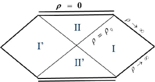
Figure 1: Penrose diagram of the black holes with $-1\leq q<0$.

Using the fact that the null vector $\boldsymbol{\gamma}$ is, from ${\rm sign}[k^{-1}(z+u)]=\epsilon^{\prime}{\rm sign}(1-\beta^{2})$, future in the present case, the right-hand side of (4.9) is generically positive. It follows that for $-1\leq q<0$, geodesics extend to infinity and the black hole metric is regular. The Penrose diagram is similar to that of the Schwarzschild black hole (Fig. 1).

On the other hand, for $q<-1$ almost all geodesics terminate at $\rho\to+\infty$. This is not a curvature singularity (the Ricci scalar (4.4) is finite), but a second horizon through which the metric cannot be generically be extended. However, as in the case of other “cold black hole” solutions of gravitating field theories with negative gravitational constant in three [20] or four [21, 22] dimensions, characterized by an infinite horizon area and vanishing Hawking temperature, the metric and the geodesics can be analytically continued across the horizon for discrete values of the model parameters. In the present case, Eq. (4.9) suggests transforming to the radial coordinate $x=\rho^{(1+q)/2}$, in terms of which the geodesic equation (4.8) can be written

$$\frac{4}{(q+1)^{2}}\left(\frac{dx}{d\tau}\right)\!^{2}+\mathbf{P}.\left(\boldsymbol{\gamma}+\boldsymbol{\beta}\,x^{m}+\boldsymbol{\alpha}\,x^{2m}\right)-\varepsilon\beta^{2}\,x^{n}\left(\rho_{0}^{2q-1}-x^{m}\right)=0\,,$$ (4.10)

where we have put

$$n=\frac{2q}{q+1}\,,\quad m=\frac{2(2q-1)}{q+1}=3n-2\,.$$ (4.11)

It is clear that Eq. (4.10) is analytic, and therefore geodesics can be extended from $x>0$ to $x<0$, if $n$ is an integer, $n>2$, corresponding to the quantization condition

$$q=-\frac{n}{n-2}\,.$$ (4.12)

Near the cold horizon $x=0$, the lapse function in (4.1) is proportional to $x^{n}$, showing that this is a multiple horizon (hence its vanishing Hawking temperature) of multiplicity $n$.

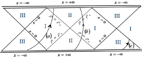
Figure 2: Penrose diagram of the cold black holes with $n$ odd; ($a$) is a normal geodesic, ($b$) and ($c$) are exceptional geodesics.

For $n$ odd, $\rho=x^{2-n}$ and $\rho^{2q-1}=x^{3n-2}$ change sign when the cold horizon is crossed from the Lorentzian region $I$ ($0<x<\rho_{0}^{-1/(n-2)}$) to the inner region $III$ ($x<0$) bounded by the spacelike singularity $x=-\infty$ ($\rho=0$). The resulting Penrose diagram is an infinite spacelike strip (Fig. 2). Using the fact that $\boldsymbol{\alpha}$ and $\boldsymbol{\gamma}$ are both future null, one can show that almost all timelike or null geodesics originate from the past spacelike singularity, cross successively the two horizons, and end at the future spacelike singularity. Exceptional timelike or null geodesics (those fine-tuned so that $\mathbf{P}=c\boldsymbol{\gamma}$ with $c>0$) do not cross the cold horizon. Exceptional geodesics with $x>0$ are time-symmetric, originating from the past singularity and ending at the future singularity after crossing twice the horizon $\rho=\rho_{0}$. Exceptional geodesics with $x<0$ either originate from the past singularity and asymptote the cold horizon, or follow the time-reversed history.

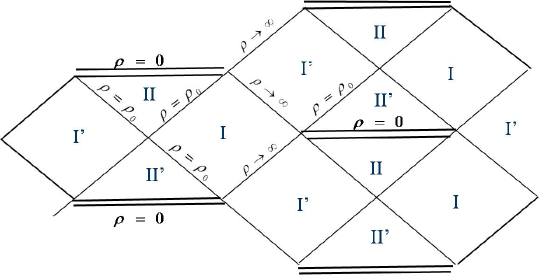
Figure 3: Penrose diagram of the cold black holes with $n$ even.

For $n$ even, analytic extension from $x>0$ to $x<0$ leads from the Lorentzian region $I$ to an isometric Lorentzian region $I^{\prime}$, so that the corresponding Penrose diagram paves the whole plane (Fig. 3). The effective potential in (4.10) is now symmetrical in $x$. Typical timelike or null geodesics either join a past singularity to a future singularity, without crossing, or crossing only once the cold horizon $x=0$, or cross periodically the cold horizon and extend to infinity.

To summarize, the solution (3.25) or (4.1) (with $k=\epsilon=-1$ and $\epsilon^{\prime}=+1$) and (3.27) corresponds to two disjoint sectors of regular black holes if the model parameters are such that $\kappa<0$, $\Lambda>\mu^{2}/4$ (ensuring from (3.26) that $\beta^{2}<0$ for $q<0$), $b=-2c$, and either $c^{2}\geq-16\kappa$ (ensuring from (3.18) that $-1\leq q<0$), or $c^{2}=-16\kappa(n-1)/n$ ($q=-n/(n-2)$) with $n>2$.

5 Mass, angular momentum and thermodynamics

The metric (4.1) is neither asymptotically flat nor asymptotically AdS, so that neither the ADM approach [23] nor the Abbott-Deser-Tekin (ADT) approach [24, 25], which involve linearization around a flat or constant curvature background, can be used to compute the conserved black hole charges, which are its mass and angular momentum. In [6] the ADT approach was extended to compute the conserved charges of a solution of topologically massive gravity linearized around an arbitrary background. This approach was further generalized in [8] to the case of TMGE, and in [26] to that of new massive gravity. However, the authors of [26] pointed out that for warped AdS₃ black holes the angular momentum obtained in these approaches was quadratic rather than linear in the black hole parameters, so that, while the mass and angular momentum obtained satisfied the first law of black hole thermodynamics and so appeared to be correct, there was a problem with the self-consistency of their derivation.

The solution to this problem was given recently in [28], generalizing an approach proposed in [27]. Warped AdS₃ black holes — and this is also true for the dilatonic black holes considered here — depend on two arbitrary parameters (integration constants). Their asymptotics are such that their metric cannot be considered to match at spacelike infinity that of any arbitrarily given background solution, except one which is infinitesimally near in parameter space to the solution under consideration. Following the generalized ADT approach of [6], one can compute the corresponding differential conserved charges, from which the finite conserved charges can be obtained as line integrals in parameter space.

The differential mass and angular momentum of our dilatonic black hole solutions are the Killing charges, defined as integrals over the boundary $\partial M$ of a spacelike hypersurface $M$

$$\delta Q(\boldsymbol{\xi})=\frac{1}{\kappa}\int_{\partial M}\sqrt{|g|}\delta{\cal F}^{0i}(\boldsymbol{\xi})dS_{i}\,,$$ (5.1)

of the superpotentials

$$\delta{\cal F}^{\mu\nu}(\boldsymbol{\xi})=\delta{\cal F}^{\mu\nu}_{g}(\boldsymbol{\xi})+\delta{\cal F}^{\mu\nu}_{e}(\boldsymbol{\xi})$$ (5.2)

associated with the Killing vectors $\boldsymbol{\xi}=\partial_{t}$ and $\boldsymbol{\xi}=\partial_{\varphi}$. In (5.2) the gravitational contribution is the Einstein superpotential given in [6] (Eq. (2.14)), and the electromagnetic contribution is obtained from that of [29] by replacing the fields canonically conjugate to the vector potential $A$ by $e^{c\phi}F$,

$$\delta{\cal F}^{\mu\nu}_{e}(\boldsymbol{\xi}) = \frac{\kappa}{\sqrt{|g|}}\delta\bigg{[}\sqrt{|g|}e^{c\phi}F^{\mu\nu}-\mu\epsilon^{\mu\nu\lambda}A_{\lambda}\bigg{]}\xi^{\rho}A_{\rho}$$ (5.3)

$$+\kappa e^{c\phi}\bigg{[}F^{\mu\nu}\xi^{\rho}+F^{\nu\rho}\xi^{\mu}+F^{\rho\mu}\xi^{\nu}\bigg{]}\delta A_{\rho}\,.$$

For a rotationally symmetric configuration, the relevant component is $\delta{\cal F}^{02}_{e}(\xi)$. The first bracket of (5.3) vanishes by virtue of (2.9), and there remains

$$\delta{\cal F}^{02}_{e}(\boldsymbol{\xi})=-\kappa F^{2a}\epsilon_{ab}\xi^{b}\delta\psi_{1}=-\kappa\zeta^{2}(\xi^{T}\psi)\delta\overline{\psi}^{0}=\frac{\zeta^{2}}{2}\bigg{[}\xi^{T}\mathbf{\Sigma}.\delta\mathbf{S}-\kappa(\delta\overline{\psi}\psi)\xi^{T}\bigg{]}^{0}\,,$$ (5.4)

as in [8]. Therefore, the Killing charges are obtained from those given there by omitting the gravitational Chern-Simons term:

$$\delta Q(\boldsymbol{\xi})=\frac{\pi\zeta}{\kappa}\left[\xi^{T}\left(\mathbf{\Sigma}.\delta\mathbf{J}+\Delta\right)\right]^{0}\,,$$ (5.5)

where $\mathbf{J}$ is the super angular momentum [7],

$$\mathbf{J}=\mathbf{X}\wedge\mathbf{X}^{\prime}+\mathbf{S}\,,$$ (5.6)

which is constant by virtue of (2.15) and (2.11), and $\Delta$ is the scalar

$$\Delta=\mathbf{X}.\delta\mathbf{X}^{\prime}-\kappa\left(\delta\overline{\psi}\psi\right)\,.$$ (5.7)

For our black hole solutions we obtain, from (3.3), (3.16) and (3.18) with $k=-1$,

$$\mathbf{J}=(1-2q)[\boldsymbol{\beta}\wedge\boldsymbol{\gamma}+2(\boldsymbol{\alpha}.\boldsymbol{\gamma})\boldsymbol{\gamma}]\,,$$ (5.8)

and,

$$\Delta=(1-2q)(2-\beta^{2})\,(\boldsymbol{\beta}.\delta\boldsymbol{\gamma})+q\delta(\boldsymbol{\beta}.\boldsymbol{\gamma})=-\beta^{2}\,\delta\left[(1-2q)v+\frac{q}{2}\rho_{0}^{2q-1}\right]\,.$$ (5.9)

We note here that, had we defined $\delta\mathbf{X}^{\prime}$ not as a differential, but as the finite (linearized) difference $\mathbf{X}^{\prime}-\mathbf{X}^{\prime}_{0}$, with $\mathbf{X}_{0}$ a given background solution, $\Delta$ would have contained in addition a non-constant contribution proportional to $(\boldsymbol{\gamma}.(\boldsymbol{\gamma}-\boldsymbol{\gamma}_{0}))\rho^{1-2q}$, which is absent here because $(\boldsymbol{\gamma}.\delta\boldsymbol{\gamma})=0$ by virtue of the constraint (3.9). So in the present case the definition of the Killing charges as differentials is essential to guarantee their conservation.

The black-hole mass and angular momentum are respectively the Killing charges for the vectors $\boldsymbol{\xi}=(-1,0)$ and $\boldsymbol{\xi}=(0,1)$,

$$M = -\frac{\pi\mu}{\kappa}\left(\delta J^{Y}+\int\Delta\right)\,,$$

$$J = \frac{\pi\mu}{\kappa}\left(\delta J^{T}-\delta J^{X}\right)\,,$$ (5.10)

where the integral over $\Delta$ is a line integral from the “vacuum” solution $v=\rho_{0}^{2q-1}=0$ to the solution under consideration. We obtain from (5.8) and (5.9):

$$M = \frac{\pi\mu\beta^{2}}{\kappa}\left[2(1-2q)v-\frac{1-3q}{2}\rho_{0}^{2q-1}\right]\,,$$ (5.11)

$$J = \frac{\pi\mu\beta^{2}}{\kappa}\frac{1-2q}{1-\beta^{2}}\,v\left(v-\rho_{0}^{2q-1}\right)\,.$$ (5.12)

Noting that for our black holes $\kappa<0$ and $\beta^{2}<0$, we find that the mass $M$ is positive in the black-hole sector $v>v_{+}$ ($>\rho_{0}^{2q-1}$), and negative in the black-hole sector $v<v_{-}$ ($<0$), while the angular momentum $J$ is positive in both sectors.

A third black-hole observable is its entropy, proportional to its horizon areal radius $r_{h}$ (computed in Appendix A),

$$S=\frac{4\pi^{2}}{\kappa}r_{h}=\frac{4\pi^{2}}{\kappa\sqrt{1-\beta^{2}}}\,\rho_{0}^{(1-q)/2}|v-\rho_{0}^{2q-1}|\,,$$ (5.13)

which is negative. The other thermodynamical observable is the Hawking temperature,

$$T=\frac{\mu(R^{2})^{\prime}(\rho_{0})}{4\pi r_{h}}=-\frac{\mu\beta^{2}\sqrt{1-\beta^{2}}(1-2q)}{4\pi}\,\frac{\rho_{0}^{(5q-3)/2}}{|v-\rho_{0}^{2q-1}|}\,.$$ (5.14)

Finally, the horizon angular velocity is

$$\Omega_{h}=-\frac{Y(\rho_{0})}{r_{h}^{2}}=\frac{1-\beta^{2}}{v-\rho_{0}^{2q-1}}\,.$$ (5.15)

This is positive in the sector $v>v_{+}$ (co-rotating black holes) and negative in the sector $v<v_{-}$ (counter-rotating black holes). Let us recall that counter-rotating black holes (whose horizon rotates in the opposite sense to the angular momentum) have previously been numerically constructed in four-dimensional Einstein-Maxwell-dilaton theory (with dilaton coupling constant larger than $\sqrt{3}$) [30], and in five-dimensional Einstein-Maxwell-Chern-Simons theory (with Chern-Simons coefficient larger than $1$) [31].

These values can be checked to be consistent with the first law of black hole thermodynamics for independent variations of the black hole parameters $v$ and $\rho_{0}$,

$$dM=TdS+\Omega_{h}dJ\,.$$ (5.16)

We also note that the Chern-Simons dilaton black holes satisfy the integral Smarr-like relation

$$M=\frac{1-3q}{2(1-2q)}TS+2\Omega_{h}J\,,$$ (5.17)

which generalizes that given in [8] for Chern-Simons black holes ($q=1$).

6 Solution of five-dimensional Einstein-Maxwell-Chern-Simons theory

Dimensional reduction of higher-dimensional field theories generically leads to the appearance of dilaton fields, so one can surmise that, at least in a domain of parameter space, the theory (2.1) results from the reduction of some higher-dimensional field theory. In [32], five-dimensional Einstein-Maxwell-Chern-Simons theory was reduced, by monopole compactification on a constant curvature two-surface, to three-dimensional Einstein-Maxwell-Chern-Simons theory with an additional constraint. This “hard” reduction led to five-dimensional solutions which included a class generated from the three-dimensional warped AdS black holes. We now show that a special “soft” reduction, where the constraint is avoided by introducing a dilaton field, leads to a subclass of the theory (2.1). Conversely, oxidation of a subclass of the solutions derived in the present paper therefore leads to non-asymptotically flat solutions of the five-dimensional theory.

Five-dimensional Einstein-Maxwell-Chern-Simons theory is defined by the action

$$S_{5}=\frac{1}{16\pi G_{5}}\int d^{5}x\bigg{[}\sqrt{|g_{(5)}|}\bigg{(}R_{(5)}-\frac{1}{4}F_{(5)}^{\mu\nu}F_{(5)\mu\nu}\bigg{)}-\frac{\gamma}{12\sqrt{3}}\epsilon^{\mu\nu\rho\sigma\lambda}F_{(5)\mu\nu}F_{(5)\rho\sigma}A_{(5)\lambda}\bigg{]}\,,$$ (6.1)

where $F_{(5)}=dA_{(5)}$, $\mu,\nu,\cdots=1,\cdots,5$, and $\gamma$ is the Chern-Simons coupling constant, the value $\gamma=1$ corresponding to minimal five-dimensional supergravity. Let us assume for the five-dimensional metric and the vector potential the warped product ansätze

$$ds_{(5)}^{2} = e^{-c\phi(x^{\gamma})}g_{\alpha\beta}(x^{\gamma})dx^{\alpha}dx^{\beta}+e^{c\phi(x^{\gamma})/2}\,a^{2}(dx^{2}+dy^{2})\,,$$

$$A_{(5)} = \sqrt{2\kappa}\,A_{\alpha}(x^{\gamma})dx^{\alpha}+\frac{e}{2}\,(xdy-ydx)\,,$$ (6.2)

where $\alpha,\beta,\gamma=1,2,3$, $x^{4}=x$, $x^{5}=y$ are the transverse space coordinates, and $a>0$ is an arbitrary scale. The constant transverse magnetic field $F_{xy}=e$ solves identically the corresponding Maxwell equations, and its contribution to the five-dimensional energy-momentum tensor is proportional to the flat transverse space metric. The remaining five-dimensional field equations reduce to three-dimensional equations deriving from the action (2.1), with $b=-2c$ and the identifications

$$\Lambda=\frac{e^{2}}{4a^{4}}\,,\quad c=4\sqrt{\frac{2\kappa}{3}}\,,\quad\mu=\frac{2\gamma e}{\sqrt{3}a^{2}}\,.$$ (6.3)

These equations are solved by (3.14), (3.25) and (3.27) with

$$q=\frac{3}{7}\,,\quad\beta^{2}=-\frac{1}{2}\left(1-\frac{3}{4\gamma^{2}}\right)\,,\quad k=-7\rho_{1}^{-4/7}\,,$$ (6.4)

Because in the present case $\kappa$ is positive and $q<1/2$, it follows from the analysis of Sect. 4 that this is a stationary solution ($g_{\rho\rho}$ is positive for $\rho>\rho_{0}$) if $\beta^{2}<0$, i.e. $\gamma>\sqrt{3}/2$. Carrying out the coordinate transformation

$$t = \sqrt{\displaystyle\frac{7}{1-\beta^{2}}}\,\tau\,,\quad\rho=(\alpha r)^{7}\,,$$

$$\varphi = \displaystyle\frac{3\alpha}{7(4\gamma^{2}-3)}\sqrt{\displaystyle\frac{8(4\gamma^{2}-1)}{7}}\displaystyle\frac{\rho_{1}^{8/7}r_{0}^{3}}{e}\,\psi\,,$$ (6.5)

with $\alpha>0$ arbitrary, and fixing $r_{1}=a$, we find that this three-dimensional solution oxidizes according to (6) to the solution of the five-dimensional theory (6.1)

$$ds_{(5)}^{2} = -\left[d\tau+\left(w-\frac{br_{0}}{r}\right)d\psi\right]^{2}+r^{2}(dx^{2}+dy^{2})$$

$$+\frac{\overline{\beta}^{2}b^{2}}{r_{0}}\left[\frac{r^{2}dr^{2}}{4r_{0}^{2}(r-r_{0})}+\frac{r_{0}^{2}(r-r_{0})}{r^{2}}\,d\psi^{2}\right]\quad\left(b=\frac{\sqrt{3}r_{0}^{2}}{\gamma e\overline{\beta}^{2}}\right)\,,$$

$$A_{(5)} = \pm\sqrt{2(1+\overline{\beta}^{2})}\left[d\tau+\left(w-\frac{br_{0}}{r}\right)d\psi\right]+\frac{e}{2}\,(xdy-ydx)$$ (6.6)

(with $\overline{\beta}^{2}=-\beta^{2}$) depending on three parameters $e$, $r_{0}$ and $w$. This solution has a bolt singularity at $r=r_{0}$, but becomes regular if $\psi$ is an angle (with period $2\pi$). Then the range of $r$ is $r>r_{0}>0$, so that the singularity at $r=0$ becomes irrelevant.

One could expect the “soft” solution (6) to reduce to the “hard” Gödel class solution of [32] in the near-bolt limit $r\to r_{0}$, where the dilaton field can be replaced by a constant. This turns out not to be possible because, for $\beta^{2}<0$ ($\gamma>\sqrt{3}/2$), the constant curvature transverse two-spaces of the Gödel class solutions are not flat but hyperbolic (with negative curvature). However we show in Appendix B that there is indeed a connection, the “double near-bolt” limit of the hard solution coinciding with the near-bolt limit of the soft solution.

7 Conclusion

We have constructed rotating magnetic solutions to the three-dimensional Einstein-Maxwell-Chern-Simons-dilaton theory defined by the action (2.1) with $b=-2c$. These include for $\kappa<0$ and $\Lambda>\mu^{2}/4$ a class of black hole solutions, which generalize the warped AdS black holes of [8]. In the range $c^{2}>-16\kappa$ of the dilaton coupling constant $c$, the regular black holes are Schwarzschild-like, with a horizon shielding a spacelike singularity. For the discrete values $c^{2}=-16\kappa(n-1)/n$ (with $n>2$), null infinity is replaced by a second multiple horizon with vanishing Hawking temperature. We have also computed the mass, angular momentum and other thermodynamic observables for these solutions. The regular black holes belong to two disjoint sectors. The black holes of the first sector have a positive mass and are co-rotating, while the black holes of the second sector have a negative mass and are counter-rotating.

We have also shown that a particular, non-black hole, subfamily of our three-dimensional solutions may be uplifted to new regular non-asymptotically flat solutions of five-dimensional Einstein-Maxwell-Chern-Simons theory. We conjecture that it might be possible to generalize such a construction, both by taking into account a five-dimensional cosmological constant, and by extending the reduction ansatz (6) to a constant curvature transverse two-space, provided that the solution-generation technique of the present paper could be extended to the case of a dilaton potential more general than the Liouville potential in (2.6).

Returning to the three-dimensional theory (2.1), we comment on our apparently arbitrary choice of the relation $b+2c=0$ between the dilaton couplings. We would not expect non-trivial closed-form solutions for dilaton couplings not satisfying this constraint, which might lead to a symmetry enhancenent of the theory. In this respect, the situation might be similar to that of four-dimensional Einstein-Maxwell-dilaton theory, which admits closed form rotating solutions only for specific values of the dilaton coupling constant $\alpha$ ($\alpha=0$ or $\alpha=\sqrt{3}$), which are precisely the values for which the symmetries of the theory are enhanced [33]. Whether this is indeed the case for our three-dimensional theory remains to be investigated.

Acknowledgments

We acknowledge discussions with Adel Bouchareb at an early stage of this work. KAM and HG would like to thank LAPTh Annecy-le-Vieux for hospitality at different stages of this work. KAM acknowledges the support of the Ministry of Higher Education and Scientific Research of Algeria (MESRS) under grant D00920140043.

Appendix A

From (2.4),

$$r^{2}=g_{\varphi\varphi}=\left[-g_{tt}\right]^{-1}(Y^{2}-R^{2})\,,$$ (A.1)

where, for the metric (4.1) with $\kappa<0$ ($q<0$, $\epsilon^{\prime}=1$, $\epsilon=-1$) and $\beta^{2}<0$,

$$g_{tt}=(1-\beta^{2})\rho^{1-q}>0\;,Y=\rho^{1-q}\left(\rho^{2q-1}-v\right)\;,R^{2}=-\beta^{2}\rho\left(\rho_{0}^{2q-1}-\rho^{2q-1}\right)\,.$$ (A.2)

Putting $x=\rho^{2q-1}$, this leads to

$$r^{2}=\frac{\rho^{1-q}}{1-\beta^{2}}\left[(1-\beta^{2})x^{2}-(2v-\beta^{2}x_{0})x+v^{2}\right]\,.$$ (A.3)

The discriminant of the quadratic polynomial in brackets

$$\Delta=-4\beta^{2}\left[-v^{2}+vx_{0}-\beta^{2}x_{0}^{2}\right]$$ (A.4)

has two roots

$$v_{\pm}(x_{0})=\left[1\pm\sqrt{1-\beta^{2}}\right]\frac{x_{0}}{2}\,.$$ (A.5)

For $v_{-}<v<v_{+}$, the discriminant is positive, so that $r^{2}$ has two roots $r_{\pm}$ which are both of the same sign as

$$2v-\beta^{2}x_{0}>2v_{-}-\beta^{2}x_{0}=\left[\sqrt{1-\beta^{2}}-1\right]x_{0}>0.$$ (A.6)

These two roots correspond to two causal singularities of the metric (4.1), which are naked because $R^{2}(x_{\pm})=Y^{2}(x_{\pm})>0$. Thus, this metric leads to regular black holes only if either $v>v_{+}$, or $v<v_{-}$. From (A.1) the corresponding horizon radii are

$$\begin{array}[]{lccc}v>v_{+}\,:&r_{h}=\displaystyle\frac{\rho_{0}^{(1-q)/2}}{\sqrt{1-\beta^{2}}}\,(v-x_{0})&>&\displaystyle\frac{\rho_{0}^{(3q-1)/2}}{\sqrt{1-\beta^{2}}}\,(\sqrt{1-\beta^{2}}-1)\,,\\ v<v_{-}\,:&r_{h}=\displaystyle\frac{\rho_{0}^{(1-q)/2}}{\sqrt{1-\beta^{2}}}\,(x_{0}-v)&>&\displaystyle\frac{\rho_{0}^{(3q-1)/2}}{\sqrt{1-\beta^{2}}}\,(\sqrt{1-\beta^{2}}+1)\,,\end{array}$$ (A.7)

where we have used $v_{+}>x_{0}>0$ and $v_{-}<0<x_{0}$.

Appendix B

The “Gödel class” solution (3.22) of [32] for $\beta^{2}<0$, with $k=-1$ (negative constant curvature transverse two-space) and vanishing five-dimensional cosmological constant ($\overline{g}=g=a\overline{\beta}^{-1}$) is

$$ds_{(5)}^{2} = -\left(dt-g\cos\chi\,d\psi\right)^{2}+g^{2}\overline{\beta}^{2}\left[d\chi^{2}+\sin^{2}\chi\,d\psi^{2}+d\theta^{2}+\sinh^{2}\theta\,d\varphi^{2}\right]\,,$$

$$A_{(5)} = \pm\sqrt{2(1+\overline{\beta}^{2})}\left(dt-g\cos\chi\,d\psi\right)+\overline{e}\,\cosh\theta\,d\varphi\quad(g=2\gamma\overline{e}/\sqrt{3})\,.$$ (B.1)

In the double near-bolt limit $\chi\to 0$, $\theta\to 0$, this goes to

$$ds_{(5)}^{2} \simeq -\left(d\overline{t}+\frac{g}{2}\chi^{2}\,d\psi\right)^{2}+g^{2}\overline{\beta}^{2}\left[d\chi^{2}+\chi^{2}\,d\psi^{2}+d\theta^{2}+\theta^{2}\,d\varphi^{2}\right]\,,$$

$$A_{(5)} \simeq \pm\sqrt{2(1+\overline{\beta}^{2})}\left(d\overline{t}+\frac{g}{2}\chi^{2}\,d\psi\right)+\frac{\overline{e}}{2}\,\theta^{2}\,d\varphi\,,$$ (B.2)

with $\overline{t}=t-g\psi$.

On the other hand, the near-bolt limit $r\to r_{0}$ of the solution (6) yields

$$ds_{(5)}^{2} \simeq -\left(d\overline{t}+\frac{b}{4}\chi^{2}\,d\psi\right)^{2}+\frac{b^{2}\overline{\beta}^{2}}{4}\left[d\chi^{2}+\chi^{2}\,d\psi^{2}+d\theta^{2}+\theta^{2}\,d\varphi^{2}\right]\,,$$

$$A_{(5)} \simeq \pm\sqrt{2(1+\overline{\beta}^{2})}\left(d\overline{t}+\frac{b}{4}\chi^{2}\,d\psi\right)+\frac{eb^{2}\overline{\beta}^{2}}{8r_{0}^{2}}\,\theta^{2}\,d\varphi\,,$$ (B.3)

where we have put $\overline{t}=\tau+(w-b)\psi$, and

$$r\simeq r_{0}(1+\chi^{2}/4)\;\;(\chi\to 0)\,,\quad x=\frac{b\overline{\beta}}{2r_{0}}\theta\cos\varphi\,,\quad y=\frac{b\overline{\beta}}{2r_{0}}\theta\sin\varphi\,.$$

The two limits (Appendix B) and (Appendix B) coincide if $g=b/2$, leading from the definitions of $g$ in (Appendix B) and of $b$ in (6) to $\overline{e}=(b^{2}\overline{\beta}^{2}/4r_{0}^{2})e$.

References

- [1]
- [2] M. Bañados, C. Teitelboim and J. Zanelli, Phys. Rev. Lett. 69 (1992) 1849; M. Bañados, M. Henneaux, C. Teitelboim and J. Zanelli, Phys. Rev. D 48 (1993) 1506 [arXiv:gr-qc/9302012].
- [3] D. Anninos, W. Li, M. Padi, W. Song and A. Strominger, JHEP 0903 (2009) 130 [arXiv:0807.3040].
- [4] S. Deser, R. Jackiw and S. Templeton, Phys. Rev. Lett. 48 (1982) 975; Ann. Phys. (NY) 140 (1982) 372.
- [5] K. Ait Moussa, G. Clément and C. Leygnac, Class. Quantum Grav. 20 (2003) L277 [arXiv:gr-qc/0303042].
- [6] A. Bouchareb and G. Clément, Class. Quantum Grav. 24 (2007) 5581 [arXiv:0706.0263].
- [7] K. Ait Moussa and G. Clément, Class. Quantum Grav. 13 (1996) 2319 [arXiv:gr-qc/9602034].
- [8] K. Ait Moussa, G. Clément, H. Guennoune and C. Leygnac, Phys. Rev. D 78 (2008) 064065 [arXiv:0807.4241].
- [9] E.A. Bergshoeff, O. Hohm and P.K. Townsend, Phys. Rev. Lett. 102 (2009) 201301 [arXiv:0901.1766].
- [10] G. Clément, Class. Quantum Grav. 26 (2009) 105015 [arXiv:0902.4634].
- [11] A. Sinha, JHEP 1006 (2010) 061 [arXiv:1003.0683].
- [12] S. Nam, J.D. Park and S.H. Yi, JHEP 1007 (2010) 058 [arXiv:1005.1619].
- [13] E. Tonni, JHEP 1008 (2010) 070 [arXiv:1006.3489].
- [14] P. Castelo Ferreira, Class. Quantum Grav. 23 (2006) 3679 [arXiv:hep-th/0506244].
- [15] P. Castelo Ferreira, “Rotating magnetic solutions for 2+1 Einstein Maxwell Chern-Simons from space-time duality”, arXiv:1107.0422 (2011).
- [16] G. Clément, Class. Quantum. Grav. 10 (1993) L49.
- [17] G. Clément, Class. Quantum. Grav. 11 (1994) L115 [arXiv:gr-qc/9404004].
- [18] J. Ehlers and W. Kundt, “Exact solutions of the gravitational field equations”, in “Gravitation, an introduction to current research”, ed. L. Witten, Wiley (New York 1962), 49.
- [19] W.J. van Stockum, Proc. Roy. Soc. Edinburgh A 57 (1937) 135.
- [20] G. Clément and A. Fabbri, Class. Quantum Grav. 16 (1999) 323 [arXiv:gr-qc/9804050].
- [21] K.A. Bronnikov, G. Clément, C.P. Constantinidis and J.C. Fabris, Phys. Lett. A 243 (1998) 121 [arXiv:gr-qc/9801050]; Grav.&Cosm. 4 (1998) 128 [arXiv:gr-qc/9804064].
- [22] G. Clément, J. Fabris and M. Rodrigues, Phys. Rev. D 79 (2009) 064021 [arXiv:0901.4543].
- [23] R. Arnowitt, S. Deser and C.W. Misner, The dynamics of general relativity, in “Gravitation: An Introduction to Current Research”, ed. L. Witten (Wiley, New York, 1962).
- [24] L.F. Abbott and S. Deser, Nucl. Phys. B 195 (1982) 76.
- [25] S. Deser and B. Tekin, Phys. Rev. Lett. 89 (2002) 101101 [arXiv:hep-th/0205318]; Phys. Rev. D 67 (2003) 084009 [arXiv:hep-th/0212292].
- [26] S. Nam, J.D. Park and S.H. Yi, Phys. Rev. D 82 (2010) 124049 [arXiv:1009.1962].
- [27] G. Barnich, Class. Quantum Grav. 20 (2003) 685 [arXiv:hep-th/0301039].
- [28] W. Kim, S. Kulkarni and S.H. Yi, Phys. Rev. Lett. 111 (2013) 081101 [arXiv:1306.2138]; Phys. Rev. D 88 (2013) 124004 [arXiv:1310.1739].
- [29] M. Bañados, G. Barnich, G. Compère and A. Gomberoff, Phys. Rev. D 73 (2006) 044006 [arXiv:hep-th/0512105].
- [30] B. Kleihaus, J. Kunz and F. Navarro-Lerida, Phys. Rev. D 69 (2004) 064028 [arXiv:gr-qc/0306058].
- [31] J. Kunz and F. Navarro-Lerida, Mod. Phys. Lett. A 21 (2006) 2621.
- [32] A. Bouchareb, C. -M. Chen, G. Clément and D. V. Gal’tsov, Phys. Rev. D 88 (2013) 084048 [arXiv:1308.6461].
- [33] D.V. Gal’tsov, A. Garcia and O. Kechkin, Class. Quantum Grav. 12 (1995) 2887 [arXiv:hep-th/9504155].