Fast Parameter Estimation in Loss Tomography for Networks of General Topology

Abstract

As a technique to investigate link-level loss rates of a computer network with low operational cost, loss tomography has received considerable attentions in recent years. A number of parameter estimation methods have been proposed for loss tomography of networks with a tree structure as well as a general topological structure. However, these methods suffer from either high computational cost or insufficient use of information in the data. In this paper, we provide both theoretical results and practical algorithms for parameter estimation in loss tomography. By introducing a group of novel statistics and alternative parameter systems, we find that the likelihood function of the observed data from loss tomography keeps exactly the same mathematical formulation for tree and general topologies, revealing that networks with different topologies share the same mathematical nature for loss tomography. More importantly, we discover that a re-parametrization of the likelihood function belongs to the standard exponential family, which is convex and has a unique mode under regularity conditions. Based on these theoretical results, novel algorithms to find the MLE are developed. Compared to existing methods in the literature, the proposed methods enjoy great computational advantages.

T1This study is partially supported by National Science Foundation of USA grant DMS-1208771, National Science Foundation of China grant 11401338, Shenzhen Fund for Basic Science grant JC201005280651A and grant JC201105201150A.

, , and

1 Introduction

Network characteristics such as loss rate, delay, available bandwidth, and their distributions are critical to various network operations and important for understanding network behaviors. Although considerable attention has been given to network measurements, due to various reasons (e.g., security, commercial interest and administrative boundary) some characteristics of the network cannot be obtained directly from a large network. To overcome this difficulty, network tomography was proposed in [1], suggesting the use of end-to-end measurement and statistical inference to estimate characteristics of a large network. In an end-to-end measurement, a number of sources are attached to the network of interest to send probes to receivers attached to the other side of the network, and paths from sources to receivers cover links of interest. Arrival orders and arrival times of the probes carry the information of the network, from which many network characteristics can be inferred statistically. Characteristics that have been estimated in this manner include link-level loss rates [2, 3, 4, 5, 6, 7, 8, 9, 10, 11, 12, 13], delay distributions [14, 15, 16, 17, 18, 19, 20, 21, 22, 23], origin-destination traffic [1, 16, 24, 25, 26, 27, 28, 29, 30, 31, 32, 33, 34, 35, 36, 37, 38], loss patterns [39], and the network topology [40]. In this paper, we focus on the problem of estimating loss rates.

Network topologies connecting sources to receivers can be divided into two classes: tree and general. A tree topology, as named, has a single source attached to the root of a multicast tree to send probes to receivers attached to the leaf nodes of the tree. A network with a general topology, however, requires a number of trees to cover all links of the network. Each tree has one source sending probes to receivers in it. Because of the use of multiple sources to send probes in a network with general topology, those nodes and receivers located at intersections of multiple trees can receive probes from multiple sources. In this case, we must consider impacts of probes sent by all sources simultaneously in order to get a good estimate. This task is much more challenging than the tree topology case.

Numerous methods have been proposed for loss tomography in a tree topology. C$\acute{a}$ceres et al. [2] used a Bernoulli model to describe the loss behavior of a link, and derived the MLE for the pass rate of a path connecting the source to a node, which was expressed as the solution of a polynomial equation [2, 3, 4]. To ease the concern of using numerical methods to solve a high degree polynomial, several papers have been published to accelerate the calculation at the price of a little accuracy loss: Zhu and Geng proposed a recursively defined estimator based on a bottom-up strategy in [11, 12]; Duffield et al. proposed a closed-form estimator in [13], which has the same asymptotic variance as the MLE to the first order. Considering the unavailability of multicast in some networks, Harfoush et al. [5] and Coates et al. [6] independently proposed the use of the unicast-based multicast to send probes to receivers, where Coates et al. also suggested the use of the EM algorithm [41] to estimate link-level loss rates.

For networks beyond a tree, however, little research has been done, although a majority of networks in practice fall into this category. Conceptually, the topology of a general network can be arbitrarily complicated. However, no matter how complicated a general topology is, it can always be covered by a group of carefully selected trees, in each of which an end-to-end experiment can be carried out independently to study the properties of the subnetwork covered by the tree. If these trees do not overlap with each other, the problem of studying the whole general network can be decomposed into a group of smaller subproblems, each for one tree. However, due to the complexity of the network topology and practical constraints, it is more than often that the selected trees overlaps significantly, i.e., some links are shared by two or more trees (see Figure 2 for example). The shared links of two selected trees induce dependence between the two trees. Simply ignoring the dependence leads to a loss of information. How to effectively integrate the information from multiple trees to achieve a joint analysis is a major challenge in network tomography of general topology.

The first effort on network tomography of general topology is due to Bu et al. [8], who attempted to extend the method in [2] to networks with general topology. Unfortunately, the authors failed to derive an explicit expression for the MLE like the one presented in [2] for this more general case. They then resorted to an iterative procedure (i.e., the EM algorithm) to search for the MLE. In addition, a heuristic method, called minimum variance weighted average (MVWA) algorithm, was also proposed in [8], which deals with each tree in a general topology separately and averages the results. The MVWA algorithm is less efficient than the EM algorithm, especially when the sample size is small. Rabbat et al. in [40] considered the tomography problem for networks with an unknown but general topology, mainly focusing on network topology identification, which is beyond the scope of our current paper.

In this paper, we provide a new perspective for the study of loss tomography, which is applicable to both tree and general topologies. Our theoretical contributions are: 1) introducing a set of novel statistics, which are complete and minimal sufficient; 2) deriving two alternative parameter systems and the corresponding re-parameterized likelihood functions, which benefit us both theoretically and computationally; 3) discovering that the loss tomography for a general topology shares the same mathematical formulation as that of a tree topology; and, 4) showing that the likelihood function belongs to the exponential family and has a unique mode (which is the MLE) under regularity conditions. Based on these theoretical results, we propose two new algorithms (a likelihood-equation-based algorithm called LE-$\xi$ and an EM-based algorithm called PCEM) to find MLE. Compared to existing methods in the literature, the proposed methods are computationally much more efficient.

The rest of the paper is organized as follows. Section 2 introduces notations for tree topologies and the stochastic model for loss rate inference. Section 3 describes a set of novel statistics and two alternative parameter systems for loss rate analysis in tree topologies. New forms of the likelihood function are established based on the novel statistics and re-parametrization. Section 4 extends the above results to general topologies. Section 5 and 6 propose two new algorithms for finding MLE of $\theta$, which enjoy great computational advantages over existing methods. Section 7 evaluates performances of the proposed methods by simulations. We conclude the article in Section 8.

2 Notations and Assumptions

2.1 Notations for Tree Topologies

We use $T=(V,E)$ to denote the multicast tree of interest, where $V=\{v_{0},v_{1},...v_{m}\}$ is a set of nodes representing the routers and switches in the network, and $E=\{e_{1},...,e_{m}\}$ is a set of directed links connecting the nodes. Two nodes connected by a directed link are called the parent node and the child node, respectively, and the direction of the arrow indicates that the parent forwards received probes to the child. Figure 1 shows a typical multicast tree. Note that the root node of a multicast tree has only one child, which is slightly different from an ordinary tree, and each non-root node has exactly one parent.

Figure 1: A multicast tree.

Each link is assigned a unique ID number ranging from $1$ to $m$, based on which each node obtains its unique ID number ranging from $0$ to $m$ correspondingly so that link $i$ connects node $i$ with its parent node. Number $0$ is reserved for the source node. In contrast to [2] and [13], whose methods are node-centric, our methods here focus on links instead. For a network with tree topology, the two reference systems are equivalent as there exists an one-to-one mapping between nodes and links: every node in the network (except for the source) has a unique parent link. For a network with general topology, however, the link-centric system is more convenient, as a node in the network may have multiple parent links.

We let $f_{i}$ denote the unique parent link, $B_{i}$ the brother links, and $C_{i}$ the child links, respectively, of link $i$. To be precise, $B_{i}$ contains all links that share the same parent node with link $i$, including link $i$ itself. A subtree $T_{i}=\{V_{i},E_{i}\}$ is defined as the subnetwork composed of link $i$ and all its descendant links. We let $R$ and $R_{i}$ denote the set of receivers (i.e., leaf nodes) in $T$ and $T_{i}$, respectively. Sometimes, we also use $R$ or $R_{i}$ to denote the leaf links of $T$ or $T_{i}$. The concrete meaning of $R$ and $R_{i}$ can be determined based on the context.

Taking the multicast tree displayed in Figure 1 as an example, we have $V=\{0,1,\cdots,7\}$, $E=\{1,2,\cdots,7\}$ and $R=\{4,5,6,7\}$. For the subtree $T_{2}$, however, we have $V_{2}=\{1,2,4,5\}$, $E_{2}=\{2,4,5\}$ and $R_{2}=\{4,5\}$. For link 2, its parent link is $f_{2}=\{1\}$, its brother links are $B_{2}=\{2,3\}$, and its child links are $C_{2}=\{4,5\}$.

2.2 Stochastic Model

In a multicast experiment, $n$ probe packages are sent from the root node $0$ to all the receivers. Let $X_{i}^{(t)}=1$ if the $t$-th probe package reached node $i$, and $0$ otherwise. The status of probes at receivers $\{X_{r}^{(t)}\}_{r\in R,1\leq t\leq n}$ can be directly observed from the multicast experiment; but, the status of probes at internal links cannot be directly observed. In the following, we use $\textbf{X}_{R}=\{X^{(t)}_{R}\}_{1\leq t\leq n}$, where $X^{(t)}_{R}=\{X^{(t)}_{r}\}_{r\in R}$, to denote the data collected in a multicast experiment in tree $T$.

In this paper, we model the loss behavior of links by the Bernoulli distribution and assume the spatial-temporal independence and temporal homogeneity for the network, i.e. the event $\{X_{i}^{(t)}=0\mid X_{f_{i}}^{(t)}=1\}$ are independent across $i$ and $t$, and

$$P(X_{i}^{(t)}=0\mid X_{f_{i}}^{(t)}=0)=1,\ P(X_{i}^{(t)}=0\mid X_{f_{i}}^{(t)}=1)=\theta_{i}.$$

We call $\theta=\{\theta_{i}\}_{i\in E}$ the link-level loss rates, and the goal of loss tomography is to estimate $\theta$ from $\textbf{X}_{R}$.

2.3 Parameter Space

In principle, $\theta_{i}$ can be any value in $[0,1]$. Thus, the natural parameter space of $\theta$ is $\Theta^{*}=[0,1]^{m}$, an $m$-dimensional closed unit cube. In this paper, however, we assume that $\theta_{i}\in(0,1)$ for every $i\in E$, and thus constrain the parameter space to $\Theta=(0,1)^{m}$, to simplify the problem. If $\theta_{i}=1$ for some $i\in E$, then the subtree $T_{i}$ is actually disconnected from the other part of the network, since no probes can go through link $i$. In this case, the loss rate of other links in $T_{i}$ are not estimable due to the lack of information. On the other hand, if $\theta_{i}=0$ for some $i\in E$, the original network of interest degenerates to an equivalent network where node $i$ is removed and all its child nodes are connected directly to node $i$’s parent node. By constraining the parameter space of $\theta$ into $\Theta$, we exclude these degenerate cases from consideration.

3 Statistics and Likelihood Function

3.1 The likelihood function and the MLE

Given the loss model for each link, we can write down the likelihood function and use the maximum likelihood principle to determine unknown parameters. That is, we aim to find the parameter value that maximizes the log-likelihood function:

$$\arg\max_{\theta\in\Theta}L(\theta)=\arg\max_{\theta\in\Theta}\sum_{x\in\Omega}n(x)\log P(x;\theta),$$ (3.1)

where $x$ stands for the observation at receivers (i.e., a realization of $X_{R}$), $\Omega=\{0,1\}^{|R|}$ is the space of all possible observations with $|R|$ denoting the size of set $R$, $n(x)$ is the number of occurrences of observation $x$, and $P(x;\theta)$ is the probability of observing $x$ given parameter value $\theta$. However, the log-likelihood function (3.1) is more symbolic than practical because of the following reasons: (1) evaluating the log-likelihood function (3.1) is an expensive operation as it needs to scan through all possible $x\in\Omega$; and, (2) the likelihood equation derived from (3.1) cannot be solved analytically, and it is often computationally expensive to pursue a numerical solution.

3.2 Internal State and Internal View

Instead of using the log-likelihood function (3.1) directly, we consider to rewrite it in a different form. Under the posited probabilistic model, the overall likelihood $P(\textbf{X}_{R}\mid\theta)$ is the product of the likelihood from each probe, i.e.,

$$P(\textbf{X}_{R}\mid\theta)=\prod_{t=1}^{n}P(X_{R}^{(t)}\mid\theta).$$

Thus, an alternative form of the overall likelihood can be obtained by explicating the likelihood of each single probe and accumulating them. Two concepts called internal state and internal view can be generated from this process.

3.2.1 Internal State

For a link $i\in E$, given the observation of probe $t$ at $R_{i}$ and $R_{f_{i}}$, we are able to partially confirm whether the probe passes link $i$. Formally, for observation $\{X_{j}^{(t)}\}_{j\in R_{i}}$, we define $Y_{i}^{(t)}=\max_{j\in R_{i}}X_{j}^{(t)}$ as the internal state of link $i$ for probe $t$. If $Y_{i}^{(t)}=1$, probe $t$ reaches at least one receiver attached to $T_{i}$, which implies that the probe passes link $i$. Furthermore, by considering $Y_{f_{i}}^{(t)}$ and $Y_{i}^{(t)}$ simultaneously, we have three possible scenarios for each internal node $i$:

• $Y_{f_{i}}^{(t)}=Y_{i}^{(t)}=1$, i.e., we observed that probe $t$ passed link $i$; or

• $Y_{f_{i}}^{(t)}=1$ and $Y_{i}^{(t)}=0$, i.e., we observed that probe $t$ reached node $f_{i}$, but we did not know whether it reached node $i$ or not; or

• $Y_{f_{i}}^{(t)}=Y_{i}^{(t)}=0$, i.e., we did not know whether probe $t$ reached node $f_{i}$ or not at all;

as $Y_{f_{i}}^{(t)}=0$ and $Y_{i}^{(t)}=1$ can never happen by definition of $Y$.

The three scenarios have different impacts on the likelihood function. Formally, define

$$E_{t,1} = \{i\in E:Y_{i}^{(t)}=1\},$$

$$E_{t,2} = \{i\in E:Y_{f_{i}}^{(t)}=1,Y_{i}^{(t)}=0\},$$

$$E_{t,3} = \{i\in E:Y_{f_{i}}^{(t)}=Y_{i}^{(t)}=0\}.$$

We have

$$P(X_{R}^{(t)}\mid\theta)=\prod_{i\in E_{t,1}}(1-\theta_{i})\prod_{i\in E_{t,2}}\xi_{i}(\theta),$$ (3.2)

where

$$\xi_{i}(\theta)=P(X_{j}=0,\ \forall\ j\in R_{i}\mid X_{f_{i}}=1;\theta)$$

represents the probability that a probe sending out from the root node of $T_{i}$ fails to reach any leaf node in $T_{i}$.

3.2.2 Internal View

Accumulating the internal states of each link in the experiment, we have

$$n_{i}(1)=\sum_{t=1}^{n}Y_{i}^{(t)},$$ (3.3)

which counts the number of probes whose pass through link $i$ can be confirmed from observations. Specifically, we define $n_{0}(1)=n$. Moreover, define

$$n_{i}(0)=n_{f_{i}}(1)-n_{i}(1),$$ (3.4)

for $\forall\ i\in E$. We call the statistics $\{n_{i}(1),n_{i}(0)\}$ the internal view of link $i$. Based on internal views, we can write the log-likelihood of $\textbf{X}_{R}$ in a more convenient form:

$$L(\theta)=\sum_{i\in E}\Big{[}n_{i}(1)\log(1-\theta_{i})+n_{i}(0)\log\xi_{i}(\theta)\Big{]}.$$

3.3 Re-parametrization

Two alternative parameter systems can be introduced to re-parameterize the above log-likelihood function. First, based on the definition of $\xi_{i}(\theta)$, we have

$$\xi_{i}(\theta)=\theta_{i}+(1-\theta_{i})\prod_{j\in C_{i}}\xi_{j}(\theta),\ \ i\in E.$$ (3.5)

Note that if $i\in R$, we have $C_{i}=\emptyset$, and (3.5) degenerates to $\xi_{i}(\theta)=\theta_{i}$. Let $\xi_{i}\triangleq\xi_{i}(\theta)$ for $i\in E$. Equation (3.5) defines a one-to-one mapping between two parameter systems $\theta=\{\theta_{i}\}_{i\in E}$ and $\xi=\{\xi_{i}\}_{i\in E}$, i.e.,

$$\Gamma:\ \Theta\mapsto\Xi,\ \xi=\Gamma(\theta)\triangleq\big{(}\xi_{1}(\theta),\cdots,\xi_{m}(\theta)\big{)},$$

where $\Theta$ and $\Xi$ are the domain and image, respectively. The inverse mapping of $\Gamma$ is

$$\Gamma^{-1}:\ \Xi\mapsto\Theta,\ \theta=\Gamma^{-1}(\xi)\triangleq\big{(}\theta_{1}(\xi),\cdots,\theta_{m}(\xi)\big{)},\ \mbox{where}$$

$$\theta_{i}(\xi)=\frac{\xi_{i}-\prod_{j\in C_{i}}\xi_{j}}{1-\prod_{j\in C_{i}}\xi_{j}},\ \ i\in E.$$ (3.6)

Using $\xi$ to replace $\theta$ in $L(\theta)$, we have the following alternative log-likelihood function with $\xi$ as parameters:

$$L(\xi)=\sum_{i\in E}\Big{[}{n_{i}(1)}\log(\frac{1-\xi_{i}}{1-\prod_{j\in C_{i}}\xi_{j}})+{n_{i}(0)\log\xi_{i}}\Big{]}.$$

Second, $L(\xi)$ can be further re-organized into

$$L(\xi) = \sum_{i\in E}n_{i}(1)\log(\frac{1-\theta_{i}(\xi)}{\xi_{i}})+\sum_{i\in E}n_{f_{i}}(1)\log\xi_{i}$$

$$= n\log\xi_{1}+\sum_{i\in E}n_{i}(1)\log\psi_{i}(\xi),$$

where $\psi_{i}(\xi)$ is defined as

$$\psi_{i}(\xi)=\left\{\begin{array}[]{ll}\log\frac{1-\theta_{i}(\xi)}{\xi_{i}},&i\in R,\\ \log\frac{\xi_{i}-\theta_{i}(\xi)}{\xi_{i}},&i\notin R.\end{array}\right.$$ (3.7)

Similarly, let $\psi_{i}\triangleq\psi(\xi)$ for $i\in E$. Equation (3.7) defines a one-to-one mapping between parameter system $\xi=\{\xi_{i}\}_{i\in E}$ and $\psi=\{\psi_{i}\}_{i\in E}$, i.e.,

$$\Lambda:\ \Xi\mapsto\Psi,\ \psi=\Lambda(\xi)\triangleq\big{(}\psi_{1}(\xi),\cdots,\psi_{m}(\xi)\big{)},$$

where $\Psi\triangleq\Lambda(\Xi)$ is the image of $\psi$. The inverse mapping of $\Lambda$ is

$$\Lambda^{-1}:\ \Psi\mapsto\Xi,\ \xi=\Lambda^{-1}(\psi)\triangleq\big{(}\xi_{1}(\psi),\cdots,\xi_{m}(\psi)\big{)}.$$

It can be shown that

$$\psi_{i}=\log P\big{(}X_{i}=1\mid X_{f_{i}}=1;\ X_{j}=0,\ \forall\ j\in R_{i}\big{)}\ \mbox{for}\ i\notin R,$$

from which the physical meaning of $\psi_{i}$ can be better understood. Using $\psi$ to replace $\xi$ in $L(\xi)$, we have the following log-likelihood function with $\psi$ as parameters:

$$L(\psi)=n\log\xi_{1}(\psi)+\sum_{i\in E}n_{i}(1)\psi_{i}.$$

To illustrate the relations of $\theta$, $\xi$ and $\psi$, let’s consider the toy network in Figure 1 with $\theta_{i}=0.1$ for $i=1,\cdots,7$. It is easy to check that:

$$\xi_{4}=\xi_{5}=\xi_{6}=\xi_{7} = 0.1,$$

$$\xi_{2}=\xi_{3} = 0.1+(1-0.1)\times 0.1^{2}=0.109,$$

$$\xi_{1} = 0.1+(1-0.1)\times 0.109^{2}\approx 0.1107;$$

$$\psi_{4}=\psi_{5}=\psi_{6}=\psi_{7} = \log\frac{1-0.1}{0.1}\approx 2.1972,$$

$$\psi_{2}=\psi_{3} = \log\frac{0.109-0.1}{0.109}\approx-2.4941,$$

$$\psi_{1} \approx \log\frac{0.1107-0.1}{0.1107}\approx-2.3366.$$

We list these concrete values in Table 1 for comparison purpose. The notations, statistics and parameter systems are summarized into Table 2 for easy reference.

Table 1: Comparing different parameter systems for the toy network in Figure 1

Link	1	2	3	4	5	6	7
$\theta$	0.1	0.1	0.1	0.1	0.1	0.1	0.1
$\xi$	$0.1092$	$0.109$	$0.109$	0.1	0.1	0.1	0.1
$\psi$	$-2.3366$	$-2.4941$	$-2.4941$	$2.1972$	$2.1972$	$2.1972$	$2.1972$

Table 2: Collection of symbols

Symbol	Meaning
$T$	the multicast tree of interest
$V$	the node set of $T$
$E$	the link set of $T$
$R$	the set of leaf nodes (receivers) or leaf links of $T$
$T_{i}$	the subtree with link $i$ as the root link
$V_{i}$	the node set of subtree $T_{i}$
$R_{i}$	the set of leaf nodes (receivers) or leaf links of $T_{i}$
$f_{i}$	the parent link of link $i$
$B_{i}$	the brother links of link $i$
$C_{i}$	the child links of link $i$
$X_{i}^{(t)}$	$X_{i}^{(t)}=1$ if probe $t$ reached node $i$, and $0$ otherwise
$Y_{i}^{(t)}$	$\max_{j\in R_{i}}X_{j}^{(t)}$
$n_{i}(1)$	$\sum_{t=1}^{n}Y_{i}^{(t)}$, number of probes that passed link $i$ for sure
$n_{i}(0)$	$n_{f_{i}}(1)-n_{i}(1)$
$\theta_{i}$	$P(X_{i}=0\mid X_{f_{i}}=1)$, the loss rate of link $i$
$\xi_{i}$	$P(X_{j}=0,\ \forall\ j\in R_{i}\mid X_{f_{i}}=1)$, the loss rate of $T_{i}$
$\psi_{i}$	$\log P(X_{i}=1\mid X_{f_{i}}=1;X_{j}=0,\ \forall\ j\in R_{i})$

4 Likelihood Function for General Networks

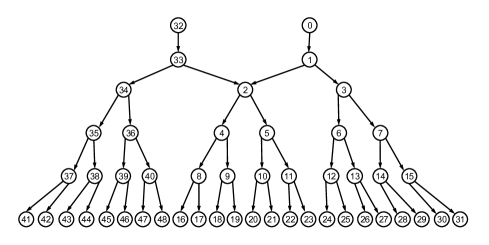
Figure 2: A 5-layer network covered by two trees.

In this section, we will extend the concept of internal view and alternative parameter systems to general networks containing multiple trees. Formally, we use $\mathscr{N}=\{T_{1},\cdots,T_{K}\}$ to denote a general network covered by $K$ multicast trees, where each multicast tree $T_{k}$ covers a subnetwork with $S_{k}$ as the root link. For example, Figure 2 illustrates a network with $K=2$, $S_{1}=0$ and $S_{2}=32$. Let $\mathscr{S}=\{S_{1},\cdots,S_{K}\}$ be the set of root links in $\mathscr{N}$.

For each tree $T_{k}$, let $\{n_{k,i}(1),n_{k,i}(0)\}$ be the internal view of link $i\in E_{k}$ in $T_{k}$ based on the $n_{k}$ probes sent out from $S_{k}$. Specially, define $n_{k,i}(1)=0$ for link $i\notin E_{k}$. The experiment on $T_{k}$ results in the following log-likelihood functions with $\theta$, $\xi$ and $\psi$ as parameters, respectively:

$$L_{k}(\theta) = \sum_{i\in E}\Big{[}n_{k,i}(1)\log(1-\theta_{i})+n_{k,i}(0)\log\xi_{i}(\theta)\Big{]},$$

$$L_{k}(\xi) = \sum_{i\in E}\Big{[}{n_{k,i}(1)}\log(\frac{1-\xi_{i}}{1-\prod_{j\in C_{i}}\xi_{j}})+{n_{k,i}(0)\log\xi_{i}}\Big{]},$$

$$L_{k}(\psi) = n_{k}\log\xi_{S_{k}}(\psi)+\sum_{i\in E}n_{k,i}(1)\psi_{i}.$$

Considering that a multicast experiment in a general network $\mathscr{N}$ is a pool of $K$ independent experiments in the $K$ trees of $\mathscr{N}$, the log-likelihood function of the whole experiment is just the summation of $K$ components, i.e.,

$$L(\theta)=\sum_{k=1}^{K}L_{k}(\theta),\ \ L(\xi)=\sum_{k=1}^{K}L_{k}(\xi)\ \ \mbox{and}\ \ L(\psi)=\sum_{k=1}^{K}L_{k}(\psi).$$

Define the internal view of link $i$ in a general network as:

$$n_{i}(1)=\sum_{k=1}^{K}n_{k,i}(1),\ \ n_{i}(0)=\sum_{k=1}^{K}n_{k,i}(0).$$ (4.1)

It is straightforward to see that

$$L(\theta) = \sum_{i\in E}\Big{[}n_{i}(1)\log(1-\theta_{i})+n_{i}(0)\log\xi_{i}(\theta)\Big{]},$$ (4.2)

$$L(\xi) = \sum_{i\in E}\Big{[}{n_{i}(1)}\log(\frac{1-\xi_{i}}{1-\prod_{j\in C_{i}}\xi_{j}})+n_{i}(0)\log\xi_{i}\Big{]},$$ (4.3)

$$L(\psi) = \sum_{k=1}^{K}n_{k}\log\xi_{S_{k}}(\psi)+\sum_{i\in E}n_{i}(1)\psi_{i}.$$ (4.4)

Note that in this general case, we have:

$$\mbox{for}\ i\in\mathscr{S},\ n_{S_{k}}(1)=n_{k};\ \mbox{and}$$

$$\mbox{for}\ i\notin\mathscr{S},\ n_{i}(0)+n_{i}(1)=\sum_{j\in F_{i}}n_{j}(1).$$

Here, $F_{i}$ stands for the unique or multiple parent links of link $i$ in the general network $\mathscr{N}$.

5 Likelihood Equation

The bijections among the the three parameter systems mean that we can switch among them freely without changing the result of parameter estimation:

    Proposition 1.

The results of likelihood inference based on the three parameter systems are equivalent, i.e.,

$$\Gamma\big{(}\arg\max_{\theta\in\Theta}L(\theta)\big{)}=\arg\max_{\xi\in\Xi}L(\xi)=\Lambda^{-1}\big{(}\arg\max_{\psi\in\Psi}L(\psi)\big{)};$$

and the likelihood equations under different parameters share the same solution, i.e.,

$$\frac{\partial L(\theta)}{\partial\theta}\Big{|}_{\theta=\theta^{*}}=0\Leftrightarrow\frac{\partial L(\xi)}{\partial\xi}\Big{|}_{\xi=\xi^{*}}=0\Leftrightarrow\frac{\partial L(\psi)}{\partial\psi}\Big{|}_{\psi=\psi^{*}}=0,$$

if $\theta^{*}\in\Theta$, or $\xi^{*}\in\Xi$, or $\psi^{*}\in\Psi$, where $\Gamma(\theta^{*})=\xi^{*}=\Lambda^{-1}(\psi^{*})$.

This flexibility provides us great theoretical and computational advantages. On the the theoretical aspect, as $\{n_{k}\}_{k=1}^{K}$ are known constants, $L(\psi)$ falls into the standard exponential family with $\psi$ as the natural parameters. Thus, based on the properties of the exponential family [42], we have the following results immediately:

    Proposition 2.

The following results hold for loss tomography:

1. Statistics $\{n_{i}(1)\}_{i\in E}$ are complete and minimal sufficient;

2. The likelihood equation $\frac{\partial L(\psi)}{\partial\psi}=0$ has at most one solution $\psi^{*}\in\Psi$;

3. If $\psi^{*}$ exists, $\psi^{*}$ (or $\theta^{*}=(\Lambda\circ\Gamma)^{-1}(\psi^{*})$) is the MLE.

On the computational aspect, the parameter system $\xi$ plays a central role. Different from the likelihood equation with $\theta$ as parameters, which is intractable, the likelihood equation with $\xi$ as parameters enjoys unique computational advantages. Let

$$r_{i}=\frac{n_{i}(1)}{n_{i}(1)+n_{i}(0)}.$$

It can be shown that the likelihood equation with $\xi$ as parameters is:

$$\xi_{i}=(1-r_{i})+r_{i}\cdot\prod_{j\in B_{i}}\xi_{j}\cdot I(i\notin\mathscr{S}),$$ (5.1)

for any link $i\in E$.

For link $i\in\mathscr{S}$, (5.1) degenerates to

$$\xi_{i}=1-r_{i}.$$

For link $i\notin\mathscr{S}$, define $\pi_{i}=\prod_{j\in B_{i}}\xi_{j}$. We note that solving $\xi_{i}$ from (5.1) is equivalent to solving the following equation about $\pi_{i}$:

$$\pi_{i}=\prod_{j\in B_{i}}\big{[}(1-r_{j})+r_{j}\cdot\pi_{i}\big{]},$$ (5.2)

which can be solved analytically when $|B_{i}|=2$, and by numerical approaches [43] when $|B_{i}|>2$.

From (5.1) and (5.2), it is transparent that only local statistics $\{r_{j}\}_{j\in B_{i}}$ are involved in estimating $\xi_{i}$. This observation leads to the following fact immediately: if a processor keeps the values of $\{r_{j}\}_{j\in B_{i}}$ in its memory, $\{\xi_{j}\}_{j\in B_{i}}$ can be effectively estimated by the processor independent of estimating the other parameters. Based on this unique property of the likelihood equation with $\xi$ as parameter, we propose a parallel procedure called “LE-$\xi$” algorithm to estimate $\theta$ (see Algorithm 1).

Algorithm 1. The LE-$\xi$ Algorithm

Hardwire requirement:

$\{\mathbb{P}_{i}\}_{i}$: a collection of processors indexed by node ID $i\in V$;

Input:

$\{r_{j}\}_{j\in E}$ with distributed storage where $\mathbb{P}_{i}$ keeps $\{r_{j}\}_{j\in C_{i}}$;

Output:

$\hat{\theta}=\{\hat{\theta}_{j}\}_{j\in E}$.

Procedure:

Operate in parallel for IDs of all non-leaf nodes $\{i\in V:i\notin R\}$

If $i\in\mathscr{S}$,

Get $\hat{\xi}_{j}=1-r_{j}$ for the unique child link $j$ of node $i$ with $\mathbb{P}_{i}$;

If $i\notin\mathscr{S}$,

Get $\hat{x}_{i}$ with $\mathbb{P}_{i}$ from $\{r_{j}\}_{j\in C_{i}}$ by solving equation below about $x$

$x=\prod_{j\in C_{i}}\big{[}(1-r_{j})+r_{j}x\big{]}$,

Get $\hat{\xi}_{j}=(1-r_{j})+r_{j}\hat{x}_{i}$ for every $j\in C_{i}$ with $\mathbb{P}_{i}$;

End parallel operation

Return $\hat{\theta}=\Gamma^{-1}(\hat{\xi})$.

The validity of the LE-$\xi$ algorithm is guaranteed by the following theorem:

    Theorem 1.

When $n_{k}\rightarrow\infty$ for all $1\leq k\leq K$, with probability one, the LE-$\xi$ algorithm has a unique solution in $\Theta=(0,1)^{m}$ that is the MLE.

Proof of Theorem 1. First, we will show that under the following regularity conditions:

$$n_{i}(1)>0,\ n_{i}(0)>0\ \ \mbox{and}\ \ \sum_{j\in F_{i}}n_{j}(1)<\sum_{j\in B_{i}}n_{j}(1)\ \ \mbox{for}\ \forall\ i\in E,$$ (5.3)

the likelihood equation with $\xi$ as parameters has a unique solution in $(0,1)^{m}$.

Note that when (5.3) holds, we have

$$0<r_{i}<1\ \ \mbox{and}\ \ \sum_{j\in B_{i}}r_{j}>1\ \mbox{for}\ \forall\ i\in E.$$

Because the Lemma 1 in [2] has shown that: if $0<c_{j}<1$ and $\sum_{j}c_{j}>1$, equation for $x$

$$x=\prod_{j}\big{[}(1-c_{j})+c_{j}x\big{]}$$

has a unique solution in $(0,1)$. It is transparent that under the regularity conditions in (5.3), equation (5.2) has a unique solution $\hat{\pi}_{i}\in(0,1)$ for every non-root link $i$. Considering that for every link $i\in E$,

$$\xi_{i}=(1-r_{i})+r_{i}\cdot\pi_{i}\cdot I(i\notin\mathscr{S}),$$

it is straightforward to see that the likelihood equation with $\xi$ as parameters has a unique solution $\hat{\xi}\in(0,1)^{m}$.

Moreover, if

$$\hat{\xi}\in\Xi,$$ (5.4)

we have $\hat{\psi}=\Lambda(\hat{\xi})\in\Psi$. Thus, based on Proposition 1 and Proposition 2, we know that if both (5.3) and (5.4) are satisfied, $\hat{\psi}$, which is the solution of the likelihood equation with $\psi$ as parameter, is the MLE. Considering the bijections among $\theta$, $\xi$ and $\psi$, this also means that $\hat{\theta}=\Gamma^{-1}(\hat{\xi})$ is the MLE.

Note that the probability that (5.3) or (5.4) fails goes to zero when $n_{k}\rightarrow\infty$ for $k=1,\cdots,K$, we complete the proof.

The large sample properties of MLE have been well studied by [2] for tree topology, where the asymptotic normality, asymptotic variance and confidence interval are established. Considering that the likelihood function keeps exactly the same form for both tree and general topology, it is natural to extend these theoretical results for MLE established in [2] to a network of general topology.

With a finite sample, there is a chance that (5.3) or (5.4) fails. In this case, the MLE of $\theta$ falls out of $\Theta$, and may be missed by the LE-$\xi$ algorithm. For example,

1. If $n_{i}(1)=0$ and $n_{i}(0)>0$, we have $\hat{\xi}_{i}=1$;

2. If $n_{i}(1)>0$ and $n_{i}(0)=0$, we have $\hat{\xi}_{i}=0$;

3. If $\sum_{j\in F_{i}}n_{j}(1)=\sum_{j\in B_{i}}n_{j}(1)>0$, we have $\hat{\theta}_{i}=0$;

4. If $\hat{\xi}_{i}\leq\hat{\pi}_{i}=\prod_{j\in B_{i}}\hat{\xi}_{j}$ (i.e., $\hat{\xi}\notin\Xi$), we have $\hat{\theta}_{i}\leq 0$.

Moreover, if $n_{i}(1)=n_{i}(0)=0$, the parameters in subtree $T_{i}$ (i.e., $\{\theta_{j}\}_{j\in T_{i}}$) are not estimable due to lack of information.

In all these cases, we cannot guarantee that the estimate from the LE-$\xi$ algorithm $\hat{\theta}$ is the global maximum in $\Theta^{*}=[0,1]^{m}$. In practice, we can increase sample size by sending additional probes to avoid this dilemma. In case that it is not realistic to send additional probes, we can simply replace $\hat{\theta}$ by the point in $\Theta^{*}$ that is the closest to $\hat{\theta}$, or search the boundary of $\Theta^{*}$ to maximize $L(\theta)$.

6 Impacts on the EM Algorithm

The above theoretical results have two major impacts to the EM algorithm widely used in loss tomography. First, as we have shown in Theorem 1, as long as regularity conditions (5.3) and (5.4) hold, likelihood function $L(\theta)$ has a unique mode in $\Theta$. In this case, the EM algorithm always converges to the MLE for any initial value $\theta^{(0)}\in\Theta$. Considering that the chance of violating (5.3) or (5.4) goes to zero with the increase of sample size, we have the following corollary for the EM algorithm immediately:

    Corollary 1.

When $n_{k}\rightarrow\infty$ for all $1\leq k\leq K$, the EM algorithm converges to the MLE with probability one for any initial value $\theta^{(0)}\in\Theta$.

Second, the formulation of the new statistics $\{n_{i}(1)\}_{i\in E}$ naturally leads to a “pattern-collapsed” implementation of the EM algorithm, which is computationally much more efficient than the widely used naive implementation where the samples are processed one by one separately. In the naive implementation of the EM algorithm, one enumerates all possible configurations of the internal links compatible with each sample carrying the information on whether the corresponding probe reached the leaf nodes or not. The complexity of the naive implementation in each E-step can be $O(n2^{m})$ in the worst case. With the pattern-collapsed implementation, however, the complexity of an E-step can be dramatically reduced to $O(m)$.

The first pattern collapsed EM algorithm is proposed by Deng et al. [23] in the context of delay tomography. The basic idea is to reorganize the observed data at receivers in delay tomography into delay patterns, and make use of a delay pattern database to greatly reduce the computational cost in the E-step. We will show below that the spirit of this method can be naturally extended to the study of loss tomography.

Define event $\{Y_{i}=0\mid Y_{f_{i}}=1\}$, or equivalently $\{X_{j}=0,\ \forall\ j\in R_{i}\mid X_{f_{i}}=1\}$, as the loss event in subtree $T_{i}$, denoted as $\mathcal{L}_{i}$. Let $L(\textbf{X}_{V};\theta)$ be the log-likelihood of the complete data where the status of probes at internal nodes are also observed, $\theta^{(r)}$ be the estimation obtained at the $r$-th iteration, the objective function to be maximized in the $(r+1)$-th iteration of the EM algorithm is:

$$Q(\theta,\theta^{(r)}) = E_{\theta^{(r)}}\big{(}L(\textbf{X}_{V};\theta)\mid\textbf{X}_{R}\big{)}=\sum_{t=1}^{n}E_{\theta^{(r)}}\big{(}L(X_{E}^{(t)};\theta)\mid X_{R}^{(t)}\big{)}$$ (6.1)

$$= \sum_{i\in E}\Big{[}n_{i}(1)\log(1-\theta_{i})+n_{i}(0)Q(\theta_{T_{i}},\theta^{(r)})\Big{]},$$

where $Q_{\mathcal{L}_{i}}(\theta_{T_{i}},\theta^{(r)})$, which is called the localized Q-function of loss event $\mathcal{L}_{i}$, is defined as:

$$Q_{\mathcal{L}_{i}}(\theta_{T_{i}},\theta^{(r)})=E_{\theta^{(r)}}\Big{[}logP(X_{T_{i}};\theta_{T_{i}})\mid\mathcal{L}_{i}\Big{]}.$$

Similar to the results for delay patterns shown in the Proposition 1 of [23], $Q_{\mathcal{L}_{i}}(\theta_{T_{i}},\theta^{(r)})$ has the following decomposition:

$$Q_{\mathcal{L}_{i}}(\theta_{T_{i}},\theta^{(r)})=\big{(}1-\psi_{i}(\theta^{(r)})\big{)}\log(\theta_{i})+\psi_{i}(\theta^{(r)})\Big{[}\log(1-\theta_{i})+\sum_{j\in C_{i}}Q_{\mathcal{L}_{j}}(\theta_{T_{j}},\theta^{(r)})\Big{]}.$$ (6.2)

Integrating (6.1) and (6.2), we have

$$Q(\theta,\theta^{(r)})=\sum_{i\in E}\Big{[}\omega_{i}(1)\log(1-\theta_{i})+\omega_{i}(0)\log(\theta_{i})\Big{]},$$

where $\{\omega_{i}(1),\omega_{i}(0)\}_{i\in E}$ are defined recursively as follows:

$\hskip 14.22636pt\bullet$ for $i\in\{S_{1},\cdots,S_{K}\}$, i.e., being one of the root links,

$$\omega_{i}(1) = n_{i}(1)+n_{i}(0)\cdot\psi_{i}(\theta^{(r)}),$$

$$\omega_{i}(0) = n_{i}(0)\cdot\big{(}1-\psi_{i}(\theta^{(r)})\big{)};$$

$\hskip 14.22636pt\bullet$ for $i\notin\{S_{1},\cdots,S_{K}\}$,

$$\omega_{i}(1) = n_{i}(1)+\sum_{j\in F_{i}}\omega_{j}(0)\cdot\psi_{j}(\theta^{(r)}),$$

$$\omega_{i}(0) = \sum_{j\in F_{i}}\omega_{j}(0)\cdot\big{(}1-\psi_{j}(\theta^{(r)})\big{)}.$$

And, the M-step is:

$$\theta_{i}^{(r+1)}=\frac{\omega_{i}(0)}{\omega_{i}(0)+\omega_{i}(1)},\ \forall\ i\in E.$$

In this paper, we refer to the EM with the pattern-collapsed implementation as PCEM to distinguish from the EM with the naive implementation, which is referred to as NEM. We have shown in [23] by simulation and theoretical analysis that PCEM is computationally much more efficient than the naive EM in the context of delay tomography. In context of loss tomography, it is easy to see from the above analysis that PCEM enjoys a complexity of $O(m)$ for each E-step, which is much more efficient than the naive EM, whose complexity can be $O(n2^{m})$ for each E-step in the worst case.

7 Simulation Studies

We verify the following facts via simulations:

1. PCEM obtains exactly same results as the naive EM for both tree topology and general topology, but is much faster;

2. LE-$\xi$ obtains exactly same results as the EM algorithm when regularity conditions (5.3) and (5.4) hold, but is much faster when the speedup from parallel computation is considered.

We carried out simulations on a 5-layer network covered by two trees as showed in Figure 2. The network has 49 nodes labeled from Node 0 to Node 48, and two sources Node 0 and Node 32. We conduct two set of simulations. One is based on the ideal model, and the other is by using network simulator 2 (ns-2, [44]).

7.1 Simulation study with the ideal model

In the first set of simulations, the data is generated from the ideal model where each link has a pre-defined constant loss rate.

To test the performance of methods on different magnitude of loss rates, we draw the link-level loss rates from Beta distributions with different parameters. The link-level loss rates $\theta=\{\theta_{i}\}_{i}$ are randomly sampled from $\text{Beta}(1,99)$, $\text{Beta}(5,995)$, $\text{Beta}(2,998)$ or $\text{Beta}(1,999)$. For example, the mean of $\text{Beta}(1,999)$ is $0.001$, so if we draw loss rates from $\text{Beta}(1,999)$, then on average we expect a $0.1\%$ link-level loss rate in the network. Given the loss rate vector $\theta$ for each network, we generated $100$ independent datasets with sample sizes $50$, $100$, $200$ and $500$, respectively. Thus, a total of $100\times 4\times 4=1600$ datasets were simulated. The sample size is evenly distributed into the two trees, e.g., the source of each tree will send out $100$ probes when sample size $n=200$.

To each of the 1600 simulated data sets, we applied NEM, PCEM, LE-$\xi$ and MVWA, respectively. The stopping rule of the EM algorithms is $\max_{i}|\theta_{i}^{(t+1)}-\theta_{i}^{(t)}|\leq 10^{-6}$, the initial values are $\theta_{i}^{(0)}=0.03$ for all $\ i\in E$. We implement MVWA algorithm by obtaining MLE estimate in each tree with LE-$\xi$ algorithm. Table 3 summarize the average running time and MSEs of these methods under different settings. From the tables, we can see that:

1. The performances of all four methods in term of MSE improve with the increase of sample size $n$ in both networks.

2. NEM and PCEM always get exactly same results.

3. The result from LE-$\xi$ is slightly different from these of the EM algorithms when sample size $n$ is as small as $100$ or $200$ due to the violation of the regularity conditions (5.3) and (5.4). When $n=500$, the results of LE-$\xi$ and EM algorithms become identical.

4. LE-$\xi$, PCEM and MVWA algorithm implemented with LE-$\xi$ are dramatically faster than NEM. For example, in simulation configuration with $\text{Beta}(1,1000)$ and sample size $n=500$, the running time of NEM is almost 2,000 times of LE-$\xi$ and PCEM.

5. The MSE of MVWA is always larger than the MSE of the other three methods, which capture the MLE. This is consistent with the result in [8].

Table 3: Performance of different methods on simulated data from ideal model on the 5-layer network in Figure 2.

		Beta(1,100)		Beta(5,1000)		Beta(2,1000)		Beta(1,1000)
$n$	Method	Time (ms)	MSE (1e-5)	Time (ms)	MSE (1e-5)	Time (ms)	MSE (1e-5)	Time (ms)	MSE (1e-5)
50	NEM	5065.50	764.49	4444.10	364.88	3396.20	188.78	2778.15	91.10
	PCEM	2.25	764.49	2.55	364.88	2.55	188.78	2.60	91.10
	LE-$\xi$	2.15	768.14	2.25	365.44	2.15	189.12	2.20	91.22
	MVWA	2.35	772.01	2.05	368.78	2.35	189.70	2.60	91.34
100	NEM	12102.90	434.39	9109.65	245.08	7323.90	89.64	7112.55	36.69
	PCEM	3.85	434.39	3.90	245.08	3.90	89.64	4.85	36.69
	LE-$\xi$	3.70	436.41	3.50	247.29	3.80	90.02	4.30	36.74
	MVWA	4.70	439.50	4.40	247.36	4.90	90.08	5.00	36.80
200	NEM	31368.95	212.79	23558.50	109.03	19184.65	44.79	16249.45	18.52
	PCEM	12.10	212.79	11.05	109.03	10.20	44.79	11.20	18.52
	LE-$\xi$	11.65	212.87	10.65	109.69	10.70	44.91	10.75	18.54
	MVWA	13.90	213.90	11.05	109.75	11.80	44.90	10.20	18.55
500	NEM	90221.95	85.17	49625.15	43.88	45402.80	14.35	43475.15	6.98
	PCEM	25.05	85.17	22.25	43.88	22.70	14.35	22.35	6.98
	LE-$\xi$	28.05	85.17	21.75	43.88	21.30	14.35	23.10	6.98
	MVWA	27.00	85.45	22.50	44.02	28.10	14.38	24.25	6.98

7.2 Simulation study by network simulator 2

We also conduct the simulation study using ns-2. We use the network topology shown in Figure 2, where the two sources located at Node 0 and Node 32 multicast probes to the attached receivers. Besides the network traffic created by multicast probing, a number of TCP sources with various window sizes and a number of UDP sources with different burst rates and periods are added at several nodes to produce cross-traffic. The TCP and UDP cross-traffic takes about $80\%$ of the total network traffic. We generated $100$ independent datasets by running the ns-2 simulation for 1, 2, 5 or 10 simulation seconds. The longer experiments generate more multicast probes samples. We record all pass and loss events for each link during the simulation, and the actual loss rates are calculated and considered as the true loss rates for calculating MSEs. Table 4 shows the average number of packets (sample size), running time of methods and MSEs for different ns-2 simulation times.

In Table 4, we observe similar results as shown in Table 3. The performances of all four methods in term of MSE improve with the increase of sample size $n$ in both networks. The result from LE-$\xi$ is slightly different from these of the EM algorithms when sample size $n$ is as small. More importantly, LE-$\xi$ and PCEM are dramatically faster than NEM.

Table 4: Performance of different methods on simulated data from network simulator 2.

Sim time ($n$)	Method	Time (ms)	MSE (1e-5)
1s (528)	NEM	54675.20	581.29
	PCEM	21.80	581.29
	LE-$\xi$	22.00	581.29
	MVWA	22.80	584.50
2s (2038)	NEM	256270.60	232.49
	PCEM	21.80	232.49
	LE-$\xi$	22.00	232.49
	MVWA	22.80	233.63
5s (5648)	NEM	745393.40	122.23
	PCEM	329.40	122.23
	LE-$\xi$	315.00	122.23
	MVWA	299.10	122.86
10s (13355)	NEM	1334478.90	75.24
	PCEM	612.90	75.24
	LE-$\xi$	612.10	75.24
	MVWA	657.00	76.59

8 Conclusion

We proposed a set of sufficient statistics called internal view and two alternative parameter systems $\xi$ and $\psi$ for loss tomography. We found that the likelihood function keeps the exactly same formulation for both tree and general topologies under all three types of parametrization ($\theta$, $\xi$ and $\psi$), and we can switch among the three parameter systems freely without changing the result of parameter estimation. We also discovered that the parameterization of the likelihood function based on $\psi$ falls into the standard exponential family, which has a unique mode in parameter space $\Psi$ under regularity conditions, and the parametrization based on $\xi$ leads to an efficient algorithm called LE-$\xi$ to calculate the MLE, which can be carried out in a parallel fashion. These results indicate that loss tomography for general topologies enjoys the same mathematical nature as that for tree topologies, and can be resolved effectively. The proposed statistics and alternative parameter systems also lead to a more efficient pattern-collapsed implementation of the EM algorithm for finding MLE, and a theoretical promise that the EM algorithm converges to the MLE with probability one when sample size is large enough. Simulation studies confirmed our theoretical analysis as well as the superiority of the proposed methods over existing methods.

References

- [1] Y. Vardi. Network Tomography: Estimating Source-Destination Traffic Intensities from Link Data. Journal of the American Statistical Association, 91(433): 365-377, 1996.
- [2] R. Cceres, N.G. Duffield, J. Horowitz, and D. Towsley. Multicastbased inference of network-internal loss characteristics. IEEE Transactions on Information Theory, 45(7): 2462-2480, 1999.
- [3] R. Cceres, N.G. Duffield, S.B. Moon, and D. Towsley. Inference of Internal Loss Rates in the MBone. In IEEE/ISOC Global Internet’99, Vol. 3, 1853-1858, 1999.
- [4] R. Cceres, N.G. Duffield, S.B. Moon, and D. Towsley. Inferring linklevel performance from end-to-end multicast measurements. Technical report, University of Massachusetts, 1999.
- [5] K. Harfoush, A. Bestavros, and J. Byers. Robust identification of shared losses using end-to-end unicast probes. In Technical Report BUCS-2000-013, Boston University, 2000.
- [6] M. Coates and R. Nowak. Unicast network tomography using EM algorthms. Technical Report TR-0004, Rice University, September 2000.
- [7] M. Coates and R. Nowak. Network loss inference using unicast end-to-end measurement. In the ITC Specialist Seminar on IP Traffic Measurement, Modeling and Management, 28-1. 2000.
- [8] T. Bu, N. Duffield, F.L. Presti, and D. Towsley. Network Tomography on General Topologies. In Proc. of ACM SIGMETRICS vol. 30, no. 1, 21-30, 2002.
- [9] F. LoPresti, D.Towsley, N.G. Duffield, and J. Horowitz. Multicast topology inference from measured end-to-end loss. IEEE Transactions on Information Theory, 48(1): 26-45, 2002.
- [10] N. Duffield, J. Horowitz, D. Towsley, W. Wei, and T. Friedman. Multicast-based loss inference with missing data. IEEE Journal of Selected Areas of Communication, 20(4): 700-713. 2002.
- [11] W. Zhu and Z. Geng. A fast method to estimate loss rates. Information Networking. Networking Technologies for Broadband and Mobile Networks, 473-482, 2004.
- [12] W. Zhu and Z. Geng. A bottom up inference of loss rate. Computer Communications, 28: 351-365, 2005.
- [13] N. Duffield, J. Horowitz, F. Presti, and D. Towsley. Explicit loss inference in multicast tomography. IEEE Transactions on Information Theory, 52(8): 3852-3855, 2006.
- [14] N.G. Duffield, J. Horowitz, F.L. Presti, and D. Towsley. Network delay tomography from end-to-end unicast measurements. Lecture Notes in Computer Science, 2170: 576-595, 2001.
- [15] F.L. Presti, N.G. Duffield, J. Horwitz, and D. Towsley. Multicast-based inference of network-internal delay distribution. IEEE/ACM Transactions on Networking, 10(6): 761-775, 2002.
- [16] G. Liang and B. Yu. Maximum pseudo likelihood estimation in network tomography. IEEE Transactionson on Signal Processing, 51(8): 2043-2053, 2003.
- [17] Y. Tsang, M. Coates, and R. Nowak. Network delay tomography. IEEE Transactionson on Signal Processing, 51(8): 2125-2136, 2003.
- [18] M.F. Shih and A.O. Hero III. Unicast-based inference of network link delay distributions with finite mixture models. IEEE Transactionson on Signal Processing, 51(8): 2219-2228, 2003.
- [19] E. Lawrence, G. Michailidis, and V. Nair. Network delay tomography using flexicast experiments. Journal of the Royal Statistical Society, Series B, 68(5): 785-813, 2006.
- [20] V. Arya, N.G. Duffield, and D. Veitch. Temporal delay tomography. The 27th Conference on Computer Communications. IEEE. 2008: 276-280, 2008.
- [21] I.H. Dinwoodie and E.A. Vance. Moment estimation in delay tomography with spatial dependence. Performance Evaluation Archive, Volume 64, Issue 7-8, 613-628, 2007.
- [22] A. Chen, J. Cao, and T. Bu. Network Tomography: Identifiability and Fourier Domain Estimation. IEEE Transcation on Signal Processing, 58(12): 6029-6039, 2010.
- [23] K. Deng, Y. Li, W. Zhu, Z. Geng, and J.S. Liu. On Delay Tomography: Fast Algorithms and Spatially Dependent Models. IEEE Transactions on Signal Processing, 60(11): 5685-5697, 2012.
- [24] M.G.H. Bell. The estimation of origin-destination matrices by constrained generalized least squares. Transportation Research, Series B 25B(1): 13-22, 1991.
- [25] D.D Ortuzar and L.G. Willumsen. Modelling transport. John Wiley and Sons, 2011.
- [26] E. Cascetta and S. Nguyen. A unified framework for estimating or updating origin/destination matrices from traffic counts. Transportation Research Part B: Methodological, 22(6): 437-455, 1988.
- [27] H. Yang, T. Sasaki, Y. Iida and Y. Asakura. Estimation of origin-destination matrices from link traffic counts on congested networks. Transportation Research Part B: Methodological, 26(6): 417-434, 1992.
- [28] H.P. Lo, N. Zhang and W.H.K. Lam. Estimation of an origin-destination matrix with random link choice proportions: a statistical approach. Transportation Research Part B: Methodological, 30(4): 309-324, 1996.
- [29] L. Bianco, G. Confessore, and P. Reverberi. A network based model for traffic sensor location with implications on O/D matrix estimates. Transportation Science, 35(1): 50-60, 2001.
- [30] C. Tebaldi and M. West. Bayesian inference on network traffic using link count data. Journal of the American Statistical Association, 93(442): 557-573, 1998.
- [31] J. Cao, D. Davis, S. Van Der Viel, B. Yu, and Z. Zu. A scalable method for estimating network traffic matrices from link counts. Technical report, Bell Labs, 41, 2001.
- [32] J. Cao, W. S. Cleveland, D. Lin, and D. X. Sun. The effect of statistical multiplexing on the long range dependence of internet packet traffic. Technical report, Bell Labs. 2002.
- [33] A. Medina, N. Taft, K. Salamatian, S. Bhattacharyya, and C. Diot. Traffic matrix estimation: existing techniques and new directions. SIGCOMM Computer Communication Review, 32(4): 161-174, 2002.
- [34] Y. Zhang, M. Roughan, C. Lund, and D. Donoho. An information-theoretic approach to traffic matrix estimation. In Proceedings of SIGCOMM, 301-312, 2003.
- [35] R. Castro, M. Coates, G. Liang, R. Nowak, and B. Yu. Network tomography: Recent developments. Statistical Science, 19(3): 499-517, 2004.
- [36] G. Liang, N. Taft, and B. Yu. A fast lightweight approach to origin-destination IP traffic estimation using partial measurements. IEEE Transactions on Information Theory, 52(6): 2634-2648, 2006.
- [37] J. Fang, Y. Vardi, and C. Zhang. An iterative tomogravity algorithm for the estimation of network traffic. In R. Liu, W. Strawderman, and C. Zhang (Eds.), Complex Datasets and Inverse Problems: Tomography, Networks and Beyond, Volume 54 of Lecture Notes-Monograph Series. IMS. 12-23, 2007.
- [38] E. M. Airoldi, and A. W. Blocker, Estimating latent processes on a network from indirect measurements. Journal of the American Statistical Association, 108(501): 149-164, 2013.
- [39] V. Arya, N.G. Duffield, and D. Veitch. Multicast inference of temporal loss characteristics. Performance Evaluation, 64(9): 1169-1180, 2007.
- [40] M. Rabbat, R. Nowak, and M. Coates. Multiple Source, Multiple Destination Network Tomography. In Proc. of IEEE Infocom 04, 1628-1639, 2004.
- [41] A. Dempster, N. Laird, and D. Rubin. Maximum likelihood from incomplete data via the EM algorithm. Journal of the Royal Statistical Society, Series B, Volume 34, 1-38, 1977.
- [42] E.L. Lehmann and G Casella. Theory of Point Estimation. Springer, 2nd edition, 1998.
- [43] M.J. Todd. The computation of fixed points and applications. Springer-Verlag, New York, 1976.
- [44] The network simulator 2 (ns-2). www.isi.edu/nsnam/ns2