High-order lattice Boltzmann models for wall-bounded flows at finite Knudsen numbers

Abstract

We analyze a large number of high-order discrete velocity models for solving the Boltzmann–BGK equation for finite Knudsen number flows. Using the Chapman–Enskog formalism, we prove for isothermal flows a relation identifying the resolved flow regimes for low Mach numbers. Although high-order lattice Boltzmann models recover flow regimes beyond the Navier–Stokes level we observe for several models significant deviations from reference results. We found this to be caused by their inability to recover the Maxwell boundary condition exactly. By using supplementary conditions for the gas-surface interaction it is shown how to systematically generate discrete velocity models of any order with the inherent ability to fulfill the diffuse Maxwell boundary condition accurately. Both high-order quadratures and an exact representation of the boundary condition turn out to be crucial for achieving reliable results. For Poiseuille flow, we can reproduce the mass flow and slip velocity up to the Knudsen number of $1$. Moreover, for small Knudsen numbers, the Knudsen layer behavior is recovered.

I Introduction

Fluid flow at very small scales has gained an increasing amount of attention recently due to its relevance for engineering applications in micro- and nanotechnologies HoTai ; Karni , e.g. microelectromechanical systems (MEMS) and porous media. The characteristic length scale $l_{0}$ of the corresponding geometries is in the range of the mean free path length $\lambda$ of the gas molecules. Such flows are often isothermal and characterized by extremely small Mach numbers. Nevertheless, these flows can become compressible because of considerable pressure gradients caused by viscous effects Arki . Based on the Chapman–Enskog (CE) expansion Chapman , the Knudsen number, defined as $K\hskip-1.49994ptn=\lambda/l_{0}$, can be considered a measure for the deviation of the flow behavior from thermodynamic equilibrium. For sufficiently large $K\hskip-1.49994ptn$ non-equilibrium effects become important and the validity of the Navier–Stokes equation breaks down. In particular, the gas-surface interaction is very complex and cannot be described by the usual no-slip boundary condition. Within the Knudsen layer Hadji the notion of the fluid as a continuum is no longer valid.

A fundamental description of hydrodynamics beyond the Navier–Stokes equation is provided by the Boltzmann equation valid for all values of $K\hskip-1.49994ptn$ and all flow regimes ref1.3 . Accurate simulations of finite $K\hskip-1.49994ptn$ flows are achieved by low-level methods solving the Boltzmann equation numerically, e.g. Direct Simulation Monte Carlo (DSMC) which is traditionally used for high Mach number flows Bird . However, the application of the DSMC method to low Mach number microflows requires a large number of samples to reduce statistical errors and is computationally very time consuming.

Therefore, reduced-order models of the Boltzmann equation, such as the Lattice–Boltzmann (LB) approach, have become attractive alternatives QianLallemand ; ChenDoolen ; ShanHe ; HeLuo . The LB method is based on a reduction of the molecular velocities to a discrete velocity set in configuration space. Standard LB models, e.g. the $D3Q19$ model with 19 discrete velocities, were developed to describe the Navier–Stokes fluid dynamics. Nowadays, they provide a well-established methodology for the computational modeling of various flow phenomena Succi . Furthermore, the LB method achieves promising results for microflow simulations Lim ; NieDoolen ; Toschi ; Ansumali ; Verhaeghe ; Reis . In particular the diffuse Maxwell boundary condition for the gas-surface interaction can be implemented at a kinetic level Gatignol ; Inamuro ; AnsumaliKarlin ; SofoneaSekerka ; Sofonea ; Meng .

A systematic extension of the LB method to high-order hydrodynamics beyond the Navier–Stokes equation has been derived by Shan et al. ShaYuaChe06 . These models are based on an expansion of the velocity space using Hermite polynomials in combination with appropriate Gauss–Hermite quadratures. First analytical solutions of the high-order LB model $D2Q16$ were presented by Ansumali et al. AnsumaliKarlinArcidiacono for Couette flow and by Kim et al. KimPitsch for Poiseuille flow. The collection of LB models in the literature has grown successively, see e.g. Refs. Shan ; ChiKar09 , but makes no claim to be complete in any sense. It was shown AnsumaliKarlinArcidiacono ; KimPitsch that a higher Gauss–Hermite quadrature order significantly improves the simulation accuracy for finite $K\hskip-1.49994ptn$ flows compared to standard LB models. However, several studies 1.10 ; Izarra ; MengZhang1 ; MengZhang2 of high-order LB methods indicate that the accuracy for finite $K\hskip-1.49994ptn$ flows does not monotonically increase with a higher Gauss–Hermite order and sensitively depends on the chosen discrete velocity set. Generally, it was observed that discrete velocity sets with an even number of velocities perform better than sets with the same Gauss–Hermite order but an odd number of velocities. Moreover there are some LB models which show considerable deviations from DSMC results for finite $K\hskip-1.49994ptn$ despite a high Gauss–Hermite quadrature order. It has been suggested that this is caused by gas-surface interactions MengZhang2 ; Brookes . The implementation of the diffuse Maxwell boundary condition using Gauss–Laguerre off-lattice quadrature models in Ref. Ambrus shows good results for Couette flow up to $Kn=0.5$. By using an alternative framework, a high-order LB model with only $27$ discrete velocities has been developed by Yudistiawan et al. Yudi10 and it was shown that the corresponding moment system is quite similar to Grad’s $26$-moment system. This off-lattice $D3Q27$ model is able to represent both, Knudsen layer effects and the Knudsen minimum for Poiseuille flow.

As an introductory example, we consider the most commonly used LB model $D3Q19$ accompanied by the diffuse Maxwell boundary condition for unknown distribution functions at solid walls. It is well-known that the $D3Q19$ model shows deviations from reference results (e.g. DSMC) for increasing $K\hskip-1.49994ptn$. As shown in Fig. 1, the normalized mass flow rate for Poiseuille flow becomes inaccurate for $K\hskip-1.49994ptn\gtrsim 0.05$. One reason for this deficiency is the inability of the $D3Q19$ velocity set to represent the diffuse Maxwell boundary condition accurately. This drawback can be measured by half-space integrals at the wall Brookes . At a solid wall any velocity moment of the distribution function can be decomposed into two parts, a half-space integral over distributions coming from the bulk region and another half-space integral (wall moment) which is given by distributions defined by the Maxwell boundary condition. For instance, the $D3Q19$ model evaluates the third wall moment $W_{zxx}$ (defined in Eq. (70)), numerically yielding an error of $28\%$. In order to achieve a better representation of the Maxwell boundary condition, however, it is mandatory that this wall moment is captured with a higher accuracy. An alternative LB model $S_{Q5E24}^{D3V15}$, see Appendix A, with $15$ velocities and the same quadrature order of $5$ yields an error of only $2\%$ for the wall moment $W_{zxx}$. Obviously, its result for the mass flow rate shown in Fig. 1 is much more accurate compared to $D3Q19$. This indicates that the LB model’s representation of the diffuse Maxwell boundary condition requires high precision. Furthermore, due to the strong restriction of the configuration space, the standard LB velocity models capture only the first order of the CE expansion and therefore the applicability for describing finite $K\hskip-1.49994ptn$ flows is limited Guo . Both models shown in Fig. 1 are not able to reproduce the Knudsen layer at solid walls where strong non-equilibrium effects are relevant. The description of finite Knudsen number flows must incorporate high-order flow regimes. It is therefore desirable to obtain high-order LB models which additionally are capable of representing the diffuse Maxwell boundary condition accurately.

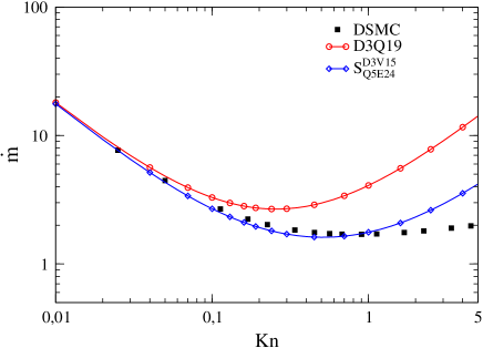
Figure 1: Normalized mass flow rate for Poiseuille flow. Both LB models $D3Q19$ and $S_{Q5E24}^{D3V15}$ are of quadrature order $5$ but differ in the accuracy of the wall moment $W_{zxx}$ and, consequently, in their capability to recover the diffuse Maxwell boundary condition.

In this work we systematically develop and investigate a large number of new high-order Gauss–Hermite LB models (on-lattice) which fulfill a constraint guaranteeing an accurate implementation of the diffuse Maxwell boundary condition. Consequently these models ensure vanishing errors of the relevant half-space integrals. We prove a theorem using the Chapman–Enskog expansion which specifies for low Mach number flows the recovered flow regimes beyond the Navier–Stokes regime depending on the Gauss–Hermite quadrature order. First simulation results for Poiseuille flow at finite $K\hskip-1.49994ptn$ show that those high-order LB models which recover the diffuse Maxwell boundary condition exactly achieve excellent agreement with DSMC results. In particular these models are able to describe Knudsen layer effects at solid walls. We emphasize that we do not resort to slip-boundary models in order to achieve these results. Finally, we recommend a preferred LB model with $96$ discrete velocities and a $7$th order Gauss-Hermite quadrature order.

The paper is organized as follows. In Sect. II, a brief review of LB models and the generation of high-order discrete velocity models is presented. In Sect. III, we derive the low Mach number theorem mentioned above. In Sect. IV, we present the systematic generation of high-order LB models with the inherent ability to capture the diffuse Maxwell boundary condition accurately. In Sect. V, we discuss the numerical implementation. In Sect. VI, we compare first simulation results for Poiseuille flow at finite $K\hskip-1.49994ptn$ with DSMC data and discuss the ability of the new LB models to describe the Knudsen layer behavior at solid walls. In Sect. VII, a summary of the major conclusions is given.

II Definition of Lattice–Boltzmann models

We consider the one-particle velocity distribution function $f(\boldsymbol{\mathbf{\xi}})$ governed by the Boltzmann equation with the Bhatnagar–Gross–Krook (BGK) collision operator,

$$\left(\partial_{t}+\boldsymbol{\mathbf{\xi}}\cdot\boldsymbol{\mathbf{\nabla}}\right)f(\boldsymbol{\mathbf{\xi}})=-\frac{1}{\tau}\left(f(\boldsymbol{\mathbf{\xi}})-f^{(0)}(\boldsymbol{\mathbf{\xi}},\rho,\boldsymbol{\mathbf{u}})\right)\;.$$ (1)

The distribution function $f(\boldsymbol{\mathbf{\xi}})$ relaxes to the equilibrium function

$$f^{(0)}(\boldsymbol{\mathbf{\xi}},\rho,\boldsymbol{\mathbf{u}})=\frac{\rho}{(2\pi\theta)^{D/2}}\exp\left(-\frac{(\boldsymbol{\mathbf{u}}-\boldsymbol{\mathbf{\xi}})^{2}}{2\theta}\right)$$ (2)

on the time scale $\tau$. At each point in space and time the macroscopic quantities are defined as velocity moments in $D$-dimensional space,

$$M_{i_{1}\ldots i_{n}}=\int d^{D}\xi\>f(\boldsymbol{\mathbf{\xi}})\>\xi_{i_{1}}\ldots\xi_{i_{n}}\;,$$ (3)

such as the density $\rho$, the velocity $\boldsymbol{\mathbf{u}}$ and the temperature $\theta$,

$$\rho = M\;,$$ (4a)

$$\rho u_{i} = M_{i}\;,$$ (4b)

$$\rho\left(D\theta+u_{i}u_{i}\right) = M_{\text{ii}}\;.$$ (4c)

Repeated indices are summed over. All quantities are dimensionless and expressed in units of characteristic scales, i.e. the length scale $l_{0}$, the reference density $\rho_{0}$, and the isothermal speed of sound $c_{0}=\sqrt{R\theta_{0}}$ with the specific gas constant $R$ and the reference temperature $\theta_{0}$. Since we focus on flows with a low Mach number $M\hskip-1.49994pta=|\boldsymbol{\mathbf{u}}|$, we assume constant temperature and set $\theta=1$ henceforth. The time $t$ as well as the relaxation time $\tau$ is expressed in units of $t_{0}=l_{0}/c_{0}$.

Following the work of Grad Grad1 ; Grad2 , Shan and He ShanHe and Shan et al. ShaYuaChe06 we discretize the velocity space by expanding the distribution function in the Hilbert space of tensorial Hermite polynomials up to an arbitrary order $N$,

$$f(\boldsymbol{\mathbf{\xi}}) \approx f^{N}(\boldsymbol{\mathbf{\xi}})=\omega(\boldsymbol{\mathbf{\xi}})\sum_{n=0}^{N}\frac{1}{n!}\>a_{i_{1}\dots i_{n}}\mathcal{H}^{(n)}_{i_{1}\dots i_{n}}(\boldsymbol{\mathbf{\xi}})\;,$$ (5)

where the Hermite polynomials $\mathcal{H}^{(n)}_{i_{1}\dots i_{n}}(\boldsymbol{\mathbf{\xi}})$ are introduced by the recurrence relation

$$\mathcal{H}^{(n+1)}_{i_{1}\dots i_{n+1}}(\boldsymbol{\mathbf{\xi}}) = \left(\xi_{i_{n+1}}-\partial_{i_{n+1}}^{(\xi)}\right)\mathcal{H}^{(n)}_{i_{1}\dots i_{n}}(\boldsymbol{\mathbf{\xi}})\;,$$ (6a)

$$\mathcal{H}^{(0)}(\boldsymbol{\mathbf{\xi}}) = 1\;.$$ (6b)

The lowest-order term of the expansion (5) is given by the weight function $\omega$,

$$\omega(\boldsymbol{\mathbf{\xi}})=\frac{1}{(2\pi)^{D/2}\text{}}e^{\left.-\boldsymbol{\mathbf{\xi}}^{2}\right/2}\;,$$ (7)

and the expansion coefficients

$$a_{i_{1}\dots i_{n}} = \int d^{D}\xi\>f^{N}(\boldsymbol{\mathbf{\xi}})\>\mathcal{H}^{(n)}_{i_{1}\dots i_{n}}(\boldsymbol{\mathbf{\xi}})\;$$ (8)

correspond to the moments of the distribution function.

II.1 Quadratures on Cartesian lattices

In the configuration space of a discrete velocity model the molecular velocities $\boldsymbol{\mathbf{\xi}}_{\alpha}$ are restricted to a Cartesian lattice $X$ with uniform spacing $c$, called lattice speed, such that the components $\xi_{\alpha i}/c$ are integer-valued. A subset of $X$ containing a number $V$ of these velocities, the stencil $S\subset X$

$$S=\left\{\left.\boldsymbol{\mathbf{\xi}}_{\alpha}\right|\alpha=1,\ldots,V\right\}\;,$$ (9)

is used with the corresponding weights $\mathrm{w}_{\alpha}$ to compute the integral in Eq. (3) by quadrature,

$$M_{i_{1}\ldots i_{n}} = \int d^{D}\xi\>\omega(\boldsymbol{\mathbf{\xi}})\>P_{i_{1}\ldots i_{n}}(\boldsymbol{\mathbf{\xi}})$$ (10)

$$= \sum_{\alpha}\mathrm{w}_{\alpha}P_{i_{1}\ldots i_{n}}(\boldsymbol{\mathbf{\xi}}_{\alpha})\;,$$

with the function $P_{i_{1}\ldots i_{n}}(\boldsymbol{\mathbf{\xi}})=f(\boldsymbol{\mathbf{\xi}})\xi_{i_{1}}\ldots\xi_{i_{n}}/\omega(\boldsymbol{\mathbf{\xi}})$. For a polynomial $P_{i_{1}\ldots i_{n}}(\boldsymbol{\mathbf{\xi}})$ of degree $Q$ the quadrature (10) is exact as long as it satisfies the orthogonality relation

$$\int d^{D}\xi\>\omega(\boldsymbol{\mathbf{\xi}})\>\mathcal{H}^{(n)}_{i_{1}\dots i_{n}}({\boldsymbol{\mathbf{\xi}}})\mathcal{H}^{(m)}_{j_{1}\dots j_{m}}({\boldsymbol{\mathbf{\xi}}})$$

$$\quad=\sum_{\alpha=1}^{V}\mathrm{w}_{\alpha}\mathcal{H}^{(n)}_{i_{1}\dots i_{n}}({\boldsymbol{\mathbf{\xi}}}_{\alpha})\mathcal{H}^{(m)}_{j_{1}\dots j_{m}}({\boldsymbol{\mathbf{\xi}}}_{\alpha})$$

$$\quad=\begin{cases}1&\textrm{if }(i_{1},\dots,i_{n})=\mathrm{perm}((j_{1},\dots,j_{m}))\\ 0&\mathrm{else}\\ \end{cases}\;,$$

$$\qquad n+m\leq Q$$ (11)

up to the $Q$th order, where perm($\boldsymbol{j}$) denotes a (odd or even) permutation of the vector $\boldsymbol{j}=(j_{1},\ldots,j_{m})$. This can be readily seen by expanding $P_{i_{1}\ldots i_{n}}(\boldsymbol{\mathbf{\xi}})$ using Hermite polynomials

$$M_{i_{1}\ldots i_{n}}=\sum_{m=0}^{Q}p_{i_{1}\dots i_{n},j_{1}\dots j_{m}}\int d^{D}\xi\>\omega(\boldsymbol{\mathbf{\xi}})\mathcal{H}^{(m)}_{j_{1}\dots j_{m}}(\boldsymbol{\mathbf{\xi}})$$ (12)

with some coefficients $p_{i_{1}\dots i_{n},j_{1}\dots j_{m}}$. If Eq. (II.1) holds, the $Q$th-order polynomial in Eq. (12) is evaluated exactly by the quadrature and hence Eq. (10) holds as well. We then refer to the stencil $S$ along with its weights $\mathrm{w}_{\alpha}$ as a discrete velocity model (DVM) with quadrature order $Q$. Note that we write the moments (10) as sums on discrete velocities, implicitly assuming a sufficiently high quadrature order, unless indicated.

A Lattice–Boltzmann (LB) model solves for the variables

$$f_{\alpha}=\mathrm{w}_{\alpha}\frac{f(\boldsymbol{\mathbf{\xi}}_{\alpha})}{\omega(\boldsymbol{\mathbf{\xi}}_{\alpha})}$$ (13)

in the LB–BGK equation

$$\left(\partial_{t}+\xi_{\alpha i}\partial_{i}\right)f_{\alpha}=-\frac{1}{\tau}\left(f_{\alpha}-f_{\alpha}^{(0)}\right)\>,$$ (14)

using a DVM for the evaluation of the macroscopic variables

$$\rho = \sum_{\alpha}f_{\alpha}\;,$$ (15a)

$$\rho u_{i} = \sum_{\alpha}f_{\alpha}\xi_{\alpha i}\;,$$ (15b)

$$\rho\left(D\theta+u_{i}u_{i}\right) = \sum_{\alpha}f_{\alpha}\xi_{\alpha i}\xi_{\alpha i}\;.$$ (15c)

The latter serve the LB model to determine the equilibrium function

$$f_{\alpha}^{(0)}(\rho,\boldsymbol{\mathbf{u}}) = \mathrm{w}_{\alpha}\frac{f^{(0)}(\boldsymbol{\mathbf{\xi}}_{\alpha},\rho,\boldsymbol{\mathbf{u}})}{\omega(\boldsymbol{\mathbf{\xi}}_{\alpha})}$$ (16)

$$= \mathrm{w}_{\alpha}\sum^{N}_{n=0}\frac{1}{n!}a^{(0)}_{i_{1}\dots i_{n}}\mathcal{H}^{(n)}_{i_{1}\dots i_{n}}({\boldsymbol{\mathbf{\xi}}}_{\alpha})\;,$$

expanded to a Hermite order $N$ where the Hermite coefficients for isothermal flows are given by

$$a^{(0)}_{i_{1}\dots i_{n}}=\rho\>u_{i_{1}}\dots u_{i_{n}}\;.$$ (17)

For any stencil $S$, the weights $\mathrm{w}_{\alpha}$ are obtained by solving the set (II.1) of linear equations. We decompose the stencil $S=\cup_{g=1}^{G}S_{g}$ into a number $G$ of velocity sets (groups), each group $S_{g}$ containing $V_{g}$ velocities (s.t. $V=\sum_{g}V_{g}$) generated by the symmetries of the lattice. These groups $S_{g}$ can be obtained by reflecting a single $\boldsymbol{\mathbf{\xi}}^{(g)}\in S_{g}$ on those hyperplanes of the lattice which reproduce the lattice itself upon reflection. Hence, the velocity weights must be identical in each group,

$$\mathrm{w}_{\alpha}=\overline{\mathrm{w}}_{g}\;\forall\left\{\alpha\left|\>\boldsymbol{\mathbf{\xi}}_{\alpha}\in S_{g}\right.\right\}\;.$$ (18)

It is efficient to rewrite Eq. (II.1) into the form

$$K_{\alpha\beta}(S)\mathrm{w}_{\beta}=0\quad\forall\alpha\;,\qquad\sum_{\alpha=1}^{V}\mathrm{w}_{\alpha}=1\;,$$ (19)

where $K$ is a symmetric matrix with elements

$$K_{\alpha\beta}(S)=\sum_{m=1}^{Q}H_{i_{1}\ldots i_{m}}^{(m)}(\boldsymbol{\mathbf{\xi}}_{\alpha})H_{i_{1}\ldots i_{m}}^{(m)}(\boldsymbol{\mathbf{\xi}}_{\beta})$$ (20)

and where the Hermite tensor indices are contracted. In view of Eq. (12), it is sufficient to solve Eq. (II.1) for $n=0$ and $m\leq Q$. Obviously, Eq. (19) then follows from Eq. (II.1) by multiplication of $\mathcal{H}^{(m)}_{i_{1}\ldots i_{m}}(\boldsymbol{\mathbf{\xi}}_{\beta})$ and summing on $m$. The reverse is true because Eq. (19) can be written, after multiplication by $\mathrm{w}_{\alpha}$, as

$$0=\mathrm{w}_{\alpha}K_{\alpha\beta}(S)\mathrm{w}_{\beta}=\sum_{m=1}^{Q}\left(\sum_{\alpha}\mathcal{H}^{(m)}_{i_{1}\ldots i_{m}}(\boldsymbol{\mathbf{\xi}}_{\alpha})\mathrm{w}_{\alpha}\right)^{2}$$

which requires that each part of the sum be zero. To obtain the matrix $K(S)$, the scalar product of two Hermite tensor polynomials is obtained by the recurrence formula (no sum on $m$)

$$\mathcal{H}^{(m+1)}_{i_{1}\dots i_{m+1}}(\boldsymbol{\mathbf{\xi}})\mathcal{H}^{(m+1)}_{i_{1}\dots i_{m+1}}(\boldsymbol{\mathbf{\eta}})=\left(\xi_{i_{m+1}}\eta_{i_{m+1}}-\xi_{i_{m+1}}\partial_{i_{m+1}}^{(\eta)}\right.$$

$$\quad\left.-\eta_{i_{m+1}}\partial_{i_{m+1}}^{(\xi)}+\partial_{i_{m+1}}^{(\xi)}\partial_{i_{m+1}}^{(\eta)}\right)\mathcal{H}^{(m)}_{i_{1}\dots i_{m}}(\boldsymbol{\mathbf{\xi}})\mathcal{H}^{(m)}_{i_{1}\dots i_{m}}(\boldsymbol{\mathbf{\eta}})\;,$$ (21)

which follows from Eq. (6).

Finding the weights $\mathrm{w}_{\alpha}$ for a stencil reduces to the task of finding the null space of the symmetric matrix $K(S)$ and normalizing according to Eq. (19). As a special feature, the matrix $K(S)$ has a parametric dependence on $c$ (through $S$) such that for some discrete values $c^{*}\in{\mathbb{R}}$ its nullity is increased. This means that by populating the stencil with sufficiently many velocity groups, we find for each quadrature order $Q$ a minimal number $G$ of velocity groups such that for $c=c^{*}$

$$\dim\ker K(S)=1\>$$ (22)

while for $c\neq c^{*}$ the matrix $K(S)$ is regular and no solution of Eq. (19) can be found. The solutions of Eq. (19) which obey Eq. (22) with $c=c^{*}$ are referred to as minimal DVMs. We only consider DVMs with positive weights. Fixing the quadrature order $Q$ and the number $V$ of velocities, there is a countable infinity of minimal DVMs, since $S$ can be chosen from the (virtually) unbounded lattice $X$. However, by introducing the integer-valued energy $E$ of a stencil and limiting it from above,

$$E=\frac{1}{2c^{2}}\sum_{\alpha=1}^{V}\boldsymbol{\mathbf{\xi}}_{\alpha}\cdot\boldsymbol{\mathbf{\xi}}_{\alpha}\leq E_{\max}$$ (23)

the number of available $Q$th-order minimal DVMs becomes finite. We are thus able to determine the complete set of minimal DVMs inside the energy sphere defined by $E\leq E_{max}$. The notation

$$S_{Q\langle Q\rangle E\langle E\rangle}^{D\langle D\rangle V\langle V\rangle}\;,\quad\textrm{e.g.\ }D3Q19\rightarrow S_{Q5E15}^{D3V19}$$ (24)

is introduced for the DVMs. As a reminder, we refer to the spatial dimension as $D$, the quadrature order as $Q$, the stencil’s energy as $E$ and the number of velocities as $V$.

	$D$	$Q$	$E_{max}$	$\#$	$V_{min}$	$\Lambda_{\mathrm{index}}$
${\cal S}_{1}$	3	7	500	4677	38	0
${\cal S}_{2}$	3	9	625	618	79	0
${\cal S}_{3}$	3	7	-	500	-	16
${\cal S}_{4}$	3	7	2500	45863	80	6245
${\cal S}_{5}$	2	7	250	1188	16	0
${\cal S}_{6}$	2	9	300	592	33	0
${\cal S}_{7}$	2	7	1000	21952	20	549

Table 1: Overview of DVM sets ${\cal S}_{n}$ which comprise a number $\#$ of minimal DVMs with dimension $D$, quadrature order $Q$, and upper limit $E_{max}$ for the stencil energy. For each set ${\cal S}_{n}$, the minimal velocity count $V_{min}$ as well as the wall accuracy index $\Lambda_{\mathrm{index}}$ (for details, see Sect. IV) is shown. The symbol ‘-’ is used where a quantity was not considered.

II.2 Discrete velocity models for bulk flow

Several sets of DVMs, denoted by ${\cal S}_{n}$, $n=1,2,\dots$, are introduced in this paper to alleviate the discussion on efficiency and accuracy of the DVMs. An overview of these sets is given in Tab. 1. Each set is defined by its dimension $D$, its quadrature order $Q$, the upper limit $E_{max}$ of the stencil’s energy and the wall accuracy index $\Lambda_{\mathrm{index}}$, see Sect.  IV.3. The wall accuracy index has the value $\Lambda_{\mathrm{index}}=0$ for the DVMs for bulk flow considered here. A set ${\cal S}_{n}$ contains a number $\#$ of minimal DVMs with $V_{min}$ being the minimal velocity count. While in one spatial dimension, it is well-known how to find $V_{min}$ for Gauss-Hermite quadratures, in higher dimensions this is not obvious. For most common quadratures in three dimensions, $V>V_{min}$. Although small values of $V$ are desirable for a high computational performance, it is unclear which choice of the stencil is the most accurate for finite $K\hskip-1.49994ptn$ number flows. It is shown in the next sections what are the essential features of a DVM for the resolution of high-order hydrodynamic regimes.

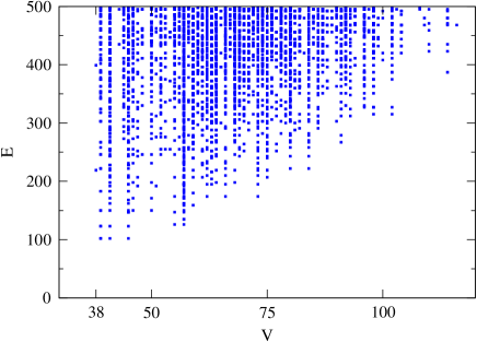
Figure 2: Complete set ${\cal S}_{1}$ of DVMs for $D=3$, $Q=7$ and $E\leq 500$, shown in the diagram of velocity count $V$ and energy $E$. Each dot represents a DVM.

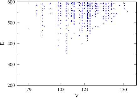
Figure 3: Complete set ${\cal S}_{2}$ of DVMs for $D=3$, $Q=9$ and $E\leq 625$, shown in the diagram of velocity count $V$ and energy $E$. Each dot represents a DVM. Within this energy range one model with a minimal number of $79$ velocities exists.

In Fig. 2, the $4677$ three-dimensional, $7$th-order DVMs of the set ${\cal S}_{1}$ are depicted. Each dot represents a DVM. Evidently, the sets of DVMs can only be complete if an upper bound on the stencil energy is provided. Here, we arbitrarily chose $E_{max}=500$ but of course this number may be increased. The lowest velocity count within ${\cal S}_{1}$ yields $V_{\min}=38$. There are two models of this kind, displayed in Tabs. 6-7. All tables of DVMs are deferred to the Appendix. In Fig. 3, we show the $618$ three-dimensional, $9$th-order DVMs of the set ${\cal S}_{2}$. The lowest velocity count yields $V_{\min}=79$. This DVM which is noted in Tab. 11 complements previously known DVMs with minimal velocities Shan . A widely used $9$th-order DVM is the one shown in Tab. 12, also known as $D3Q121$ Meng .

The so-called DVMs for wall-bounded flows of the sets ${\cal S}_{3}$ and ${\cal S}_{4}$ ($\Lambda_{\mathrm{index}}>0$) will be discussed in Sect. IV.3. Candidates of the sets ${\cal S}_{5}$, ${\cal S}_{6}$, and ${\cal S}_{7}$, which concern the popular research area of LB models in $2$ spatial dimensions, are given in Appendix B. In the sequel, we consider three spatial dimensions, $D=3$.

III Lattice–Boltzmann hydrodynamics

In this Section we study the capability of LB models with Gauss–Hermite quadrature order $Q$ and Hermite order $N$ to capture isothermal ($\theta=1$) microflows beyond the Navier–Stokes flow regime by using the Chapman–Enskog (CE) expansion. We restrict our analysis to low $M\hskip-1.49994pta$ flows. The flow phenomena thus described bear fixed values of the Reynolds number $Re$, $K\hskip-1.49994ptn$ and $M\hskip-1.49994pta$ where $M\hskip-1.49994pta\ll 1$ is a small number allowing an expansion.

By taking moments of the discrete LB–BGK equation (14) with respect to the discrete particle velocities ${\boldsymbol{\mathbf{\xi}}}_{\alpha}$ macroscopic moment equations can be derived. For the density $\rho$ and the momentum $\rho{\bf u}$, we obtain the evolution equations

$$\partial_{t}\rho+\partial_{i}\left(\rho u_{i}\right) =0$$ (25a)

$$\partial_{t}\left(\rho u_{i}\right)+\partial_{j}\Pi_{ij} =0$$ (25b)

with the momentum flux tensor

$$\Pi_{ij} =\sum_{\alpha}f_{\alpha}\xi_{\alpha i}\xi_{\alpha j}\;.$$ (26)

Equations (25a) and (25b) represent mass and momentum conservation, respectively, guaranteed by invariants of the BGK collision operator. Corresponding equations for higher moments, e.g. $\Pi_{ij}$, are derived by taking moments of Eq. (14) with more than one particle velocity $\boldsymbol{\mathbf{\xi}}_{\alpha}$.

III.1 Chapman–Enskog analysis

The CE analysis Chapman is a perturbative method to solve the Boltzmann equation and is based on the assumption that the distribution function $f_{\alpha}$ deviates only slightly from the equilibrium $f^{(0)}_{\alpha}$. The CE expansion introduces a small parameter $\epsilon$ into the collision time $\tau\to\epsilon\tau$ which controls the perturbative analysis and is absorbed into $\tau$ after finishing the analysis. Physically, the parameter $\epsilon$ may be identified with the Knudsen number, which measures the deviation from equilibrium. The first, second, and third orders correspond to the Navier–Stokes, the Burnett, and Super–Burnett flow regimes, respectively. Consequently the LB–BGK equation (14) becomes

$$\left(\partial_{t}+\xi_{\alpha i}\partial_{i}\right)f_{\alpha} =-\frac{1}{\epsilon\tau}\left(f_{\alpha}-f^{(0)}_{\alpha}\right)$$ (27)

and the distribution function is expanded in powers of $\epsilon$

$$f_{\alpha} =f^{(0)}_{\alpha}+\epsilon f^{(1)}_{\alpha}+\epsilon^{2}f^{(2)}_{\alpha}+\dots\text{ .}$$ (28)

The CE expansion is a multiple-scale expansion of both $f$ and $t$

$$\partial_{t}=\partial^{(0)}_{t}+\epsilon\partial^{(1)}_{t}+\epsilon^{2}\partial^{(2)}_{t}+\dots$$ (29)

with the solvability conditions

$$\sum_{\alpha}f^{(n)}_{\alpha} =0\;,\quad n\geq 1\;,$$ (30a)

$$\sum_{\alpha}f^{(n)}_{\alpha}\xi_{\alpha i} =0\;,\quad n\geq 1\;.$$ (30b)

Therefore, high-order contributions $f^{(n)}_{\alpha}(n\geq 1)$ of the CE expansion do not contribute to the macroscopic density and flow velocity. By inserting the CE ansatz (28) and (29) into the Boltzmann equation (27) we find the general solution for $n\geq 1$

$$f^{(n)}_{\alpha} =-\tau\left[\left(\partial^{(0)}_{t}+\xi_{\alpha i}\partial_{i}\right)f^{(n-1)}_{\alpha}+\partial^{(1)}_{t}f^{(n-2)}_{\alpha}\right.$$

$$\qquad\qquad\left.+\dots+\partial^{(n-1)}_{t}f^{(0)}_{\alpha}\right]$$ (31)

$$=-\tau\left[\partial_{i}\xi_{\alpha i}f^{(n-1)}_{\alpha}+\sum_{m=0}^{n-1}\partial^{(m)}_{t}f^{(n-m-1)}_{\alpha}\right].$$

Furthermore, the solvability conditions (30) are equivalent to the relations

$$\partial^{(0)}_{t}\begin{bmatrix}\rho\\ u_{i}\end{bmatrix} = \begin{bmatrix}-\partial_{i}\left(\rho u_{i}\right)\\ -u_{j}\partial_{j}u_{i}-\frac{1}{\rho}\partial_{i}\rho\end{bmatrix}$$ (32a)

$$\partial^{(n)}_{t}\begin{bmatrix}\rho\\ u_{i}\end{bmatrix} = \begin{bmatrix}0\\ -\frac{1}{\rho}\partial_{j}\Pi^{(n)}_{ij}\end{bmatrix}\;,\quad n\geq 1\;,$$ (32b)

where

$$\Pi^{(n)}_{ij} =\sum_{\alpha}f^{(n)}_{\alpha}\xi_{\alpha i}\xi_{\alpha j}\;.$$ (33)

The CE analysis is expected to be valid for flow regimes where the system is not too far from equilibrium Harris .

III.2 Navier-Stokes and Burnett flow regimes

The Navier–Stokes momentum flux tensor $\Pi^{(1)}_{ij}$ can be calculated by taking the second moment of Eq. (III.1) for $n=1$

$$\Pi^{(1)}_{ij} =-\tau\left(\partial^{(0)}_{t}\Pi^{(0)}_{ij}+\partial_{k}Q^{(0)}_{ijk}\right)$$ (34)

with

$$Q^{(n)}_{ijk} =\sum_{\alpha}f^{(n)}_{\alpha}\xi_{\alpha i}\xi_{\alpha j}\xi_{\alpha k}\;.$$ (35)

Using Hermite polynomials and the orthogonality relation (II.1) we obtain

$$\Pi^{(0)}_{ij} =\rho\delta_{ij}+\rho u_{i}u_{j}$$ (36)

and

$$Q^{(0)}_{ijk} =\sum_{\alpha}f^{(0)}_{\alpha}\xi_{\alpha i}\xi_{\alpha j}\xi_{\alpha k}$$ (37)

$$=\sum_{\alpha}\mathrm{w}_{\alpha}\sum^{N}_{n=0}\frac{1}{n!}a^{(0)}_{i_{1}i_{2}\dots i_{n}}\mathcal{H}^{(n)}_{i_{1}i_{2}\dots i_{n}}({\boldsymbol{\mathbf{\xi}}}_{\alpha})$$

$$\qquad\times\left[\mathcal{H}^{(3)}_{ijk}({\boldsymbol{\mathbf{\xi}}}_{\alpha})+\mathcal{H}^{(1)}_{i}({\boldsymbol{\mathbf{\xi}}}_{\alpha})\delta_{jk}\right.$$

$$\left.\qquad\qquad+\mathcal{H}^{(1)}_{j}({\boldsymbol{\mathbf{\xi}}}_{\alpha})\delta_{ik}+\mathcal{H}^{(1)}_{k}({\boldsymbol{\mathbf{\xi}}}_{\alpha})\delta_{ij}\right]$$

$$=\rho\left[u_{i}\delta_{jk}+u_{j}\delta_{ik}+u_{k}\delta_{ij}\right]+\rho u_{i}u_{j}u_{k}\;.$$ (38)

Inserting these results into Eq. (34) and evaluating the time derivative with respect to Eq. (32a) yields the Navier–Stokes momentum flux tensor $\Pi^{(1)}_{ij}$ for isothermal flows,

$$\Pi^{(1)}_{ij} =-\tau\rho\left(\partial_{i}u_{j}+\partial_{j}u_{i}\right).$$ (39)

The standard LB models with accuracy order $Q=5$ (e.g. D3Q19) do not capture the last term in Eq. (38) and thus cause an error $|\Delta\Pi^{(1)}_{ij}|=\tau\left|\partial_{k}\left(\rho u_{i}u_{j}u_{k}\right)\right|=\mathcal{O}\left(M\hskip-1.49994pta^{3}\right)$ Qian . On the other hand, if a DVM with quadrature order $Q\geq 6$ and Hermite order $N=3$ is used, we exactly recover the Navier–Stokes momentum flux tensor $\Pi^{(1)}_{ij}$. Evidently, the momentum flux tensor is $\mathcal{O}\left(M\hskip-1.49994pta\right)$ and higher-order $M\hskip-1.49994pta$ terms do not contribute when considering low $M\hskip-1.49994pta$ values.

The Burnett momentum flux tensor $\Pi^{(2)}_{ij}$ can be calculated by taking the second moment of Eq. (III.1) for $n=2$

$$\Pi^{(2)}_{ij} =-\tau\left(\partial^{(0)}_{t}\Pi^{(1)}_{ij}+\partial^{(1)}_{t}\Pi^{(0)}_{ij}+\partial_{k}Q^{(1)}_{ijk}\right).$$ (40)

The third moment of Eq. (III.1) for $n=1$ yields

$$Q^{(1)}_{ijk} =-\tau\left(\partial^{(0)}_{t}Q^{(0)}_{ijk}+\partial_{n}R^{(0)}_{ijkn}\right)$$ (41)

with

$$R^{(0)}_{ijkn} =\sum_{\alpha}f^{(0)}_{\alpha}\xi_{\alpha i}\xi_{\alpha j}\xi_{\alpha k}\xi_{\alpha n}\;.$$ (42)

By applying the Hermite polynomial the tensor $R^{(0)}_{ijkn}$ can be expressed as

$$R^{(0)}_{ijkn} =\rho\left(\delta_{ij}\delta_{kn}+\delta_{ik}\delta_{jn}+\delta_{in}\delta_{jk}\right)$$

$$\quad+\rho(u_{i}u_{j}\delta_{kn}+u_{i}u_{k}\delta_{jn}+u_{i}u_{n}\delta_{jk}+u_{j}u_{k}\delta_{in}$$

$$\quad+u_{j}u_{n}\delta_{ik}+u_{k}u_{n}\delta_{ij})+\rho u_{i}u_{j}u_{k}u_{n}\;.$$ (43)

Inserting this result together with relation (38) into Eq. (41) we can compute the tensor $Q^{(1)}_{ijk}$, which is required for the evaluation of $\Pi^{(2)}_{ij}$. After an extensive calculation of all terms in Eq. (40) by considering the multiple-scale time derivatives $\partial^{(0)}_{t}$ and $\partial^{(1)}_{t}$ we obtain the Burnett momentum flux tensor for isothermal flows,

$$\Pi^{(2)}_{ij} =2\rho\tau^{2}\bigg{[}\left(\partial_{k}u_{i}\right)\left(\partial_{k}u_{j}\right)$$

$$\quad\quad+\left.\frac{1}{\rho^{2}}\left(\partial_{i}\rho\right)\left(\partial_{j}\rho\right)-\frac{1}{\rho}\partial_{i}\partial_{j}\rho\right].$$ (44)

The Burnett tensor for an incompressible flow field is $\Pi^{(2)}_{ij}={\cal O}(M\hskip-1.49994pta^{2})$ and thus does not contribute to the momentum dynamics in the low $M\hskip-1.49994pta$ regime. However, for finite $K\hskip-1.49994ptn$ the flow behavior can become compressible even for low $M\hskip-1.49994pta$ Arki and in that case we obtain contributions from the last term of Eq. (III.2). We will show in the following Section that these low $M\hskip-1.49994pta$ terms are recovered even for LB models with accuracy order $Q=5$.

III.3 Low–Mach truncation error

Depending on the quadrature accuracy order $Q$ a LB model is able to recover different flow regimes. In this Section we analyze the quadrature error with respect to the power of $M\hskip-1.49994pta$ and discuss the ability to capture high-order flow regimes especially for low $M\hskip-1.49994pta$ flows. For this purpose we consider the $k$th moment of the $n$th CE level, which is defined by

$$M^{(n)}_{i_{1}\dots i_{k}} =\sum_{\alpha}f^{(n)}_{\alpha}\xi_{\alpha i_{1}}\dots\xi_{\alpha i_{k}}\;,$$ (45)

where $k\geq 2$ because of the solvability conditions (30). An equation for this moment can be derived by taking the $k$th moment of Eq. (III.1) with respect to the discrete particle velocities ${\boldsymbol{\mathbf{\xi}}}_{\alpha}$

$$M^{(n)}_{i_{1}\dots i_{k}} =-\tau\left[\partial^{(0)}_{t}M^{(n-1)}_{i_{1}\dots i_{k}}+\partial^{(1)}_{t}M^{(n-2)}_{i_{1}\dots i_{k}}+\dots\right.$$

$$\left.\quad\quad+\partial^{(n-1)}_{t}M^{(0)}_{i_{1}\dots i_{k}}+\partial_{j}M^{(n-1)}_{i_{1}\dots i_{k}j}\right].$$ (46)

Based on this relation it can be easily shown by induction that the moment $M^{(n)}_{i_{1}\dots i_{k}}$ is completely determined by moments of the equilibrium distribution. We assume that the moment $M^{(n)}_{i_{1}\dots i_{k}}(\partial^{(0)}\rho,\partial_{j_{1}}^{(1)}\rho,\partial_{j_{1}j_{2}}^{(2)}\rho,...,\partial^{(0)}u_{i},\partial_{j_{1}}^{(1)}u_{i},\partial_{j_{1}j_{2}}^{(2)}u_{i},...)$ is an algebraic expression of $\rho$, $u_{i}$ and their spatial derivatives, where $\partial^{(0)}=1$ and $\partial_{j_{1}\dots j_{q}}^{(q)}=\partial_{j_{1}}\dots\partial_{j_{q}}$. By using the relations (32) for the multiple-scale time derivatives the equation for $M^{(n)}_{i_{1}\dots i_{k}}$ can be written as

$$M^{(n)}_{i_{1}\dots i_{k}}= -\tau\bigg{[}\partial^{(0)}_{t}M^{(n-1)}_{i_{1}\dots i_{k}}$$

$$-\frac{1}{\rho}\sum_{m=1}^{n-1}\sum_{q}\frac{\partial M^{(n-m-1)}_{i_{1}\dots i_{k}}}{\partial(\partial_{j_{1}\dots j_{q}}^{(q)}u_{s})}\partial_{j_{1}\dots j_{q}}^{(q)}\left(\partial_{r}\Pi^{(m)}_{rs}\right)$$

$$+\partial_{j}M^{(n-1)}_{i_{1}\dots i_{k}j}\bigg{]}.$$ (49)

The sum on $q\geq 0$ in Eq. (III.3) accounts for all derivatives of $\rho$ and $u_{i}$ the moment $M^{(n)}_{i_{1}...i_{k}}$ depends on. Because of a finite accuracy order of the Gauss–Hermite quadrature higher moments of the CE expansion are only approximately captured and therefore high-order flow regimes are not accurately recovered. In order to discuss such a truncation error for a moment $M^{(n)}_{i_{1}\dots i_{k}}$ we define the quadrature error

$$\Delta M^{(n)}_{i_{1}\dots i_{k}} =M^{(n)}_{i_{1}\dots i_{k}}-M^{(n)\mathrm{DVM}}_{i_{1}\dots i_{k}},$$ (50)

where $M^{(n)\mathrm{DVM}}_{i_{1}\dots i_{k}}$ is a possibly inaccurate moment, calculated by a $\mathrm{DVM}$.

Due to the fact that a general CE moment $M^{(n)}_{i_{1}\dots i_{k}}$ can be expressed by equilibrium moments it is important to consider, in a first step, the quadrature error for equilibrium moments

$$M^{(0)}_{i_{1}\dots i_{k}} =\sum_{\alpha}f^{(0)}_{\alpha}\xi_{\alpha i_{1}}\dots\xi_{\alpha i_{k}},$$ (51)

with the equilibrium function given by Eq. (16). Note that the Hermite coefficients, see Eq. (17), yield

$$a^{(0)}_{i_{1}\dots i_{n}}=\mathcal{O}\left(M\hskip-1.49994pta^{n}\right)\;.$$ (52)

The product $\xi_{\alpha i_{1}}\dots\xi_{\alpha i_{k}}$ in (51) can be expressed by the Hermite polynomial $\mathcal{H}^{(k)}_{i_{1}\dots i_{k}}(\boldsymbol{\mathbf{\xi}}_{\alpha})$, by $\mathcal{H}^{(k-2)}_{i_{1}\dots i_{k-2}}(\boldsymbol{\mathbf{\xi}}_{\alpha})$, and terms with lower-order Hermite polynomials

$$\xi_{\alpha i_{1}}\dots\xi_{\alpha i_{k}}=\mathcal{H}^{(k)}_{i_{1}\dots i_{k}}(\boldsymbol{\mathbf{\xi}}_{\alpha})$$

$$\quad+\sum_{r<s}\mathcal{H}^{(k-2)}_{i_{1}\dots i_{r-1}i_{r+1}\dots i_{s-1}i_{s+1}\dots i_{k}}(\boldsymbol{\mathbf{\xi}}_{\alpha})\>\delta_{i_{r}i_{s}}+\dots\;.$$ (53)

Therefore we obtain

$$M^{(0)}_{i_{1}\dots i_{k}}=\sum^{N}_{n=0}\frac{1}{n!}a^{(0)}_{j_{1}\dots j_{n}}\sum_{\alpha}\mathrm{w}_{\alpha}\left[\mathcal{H}^{(n)}_{j_{1}\dots j_{n}}(\boldsymbol{\mathbf{\xi}}_{\alpha})\mathcal{H}^{(k)}_{i_{1}\dots i_{k}}(\boldsymbol{\mathbf{\xi}}_{\alpha})+\sum_{r<s}\delta_{i_{r}i_{s}}\mathcal{H}^{(n)}_{j_{1}\dots j_{n}}(\boldsymbol{\mathbf{\xi}}_{\alpha})\mathcal{H}^{(k-2)}_{i_{1}\dots i_{r-1}i_{r+1}\dots i_{s-1}i_{s+1}\dots i_{k}}(\boldsymbol{\mathbf{\xi}}_{\alpha})+\dots\right].$$ (54)

An exact evaluation of the moment $M^{(0)}_{i_{1}\dots i_{k}}$ requires a sufficiently high Hermite order $N\geq k$ of the equilibrium (16) to ensure that the contributions of all Hermite polynomials in the brackets are included Shan . Due to the orthogonality relation (II.1) higher Hermite polynomials in the equilibrium, $\mathcal{H}^{(n)}_{i_{1}\dots i_{n}}$ with $n>k$, do not contribute to the moment $M^{(0)}_{i_{1}\dots i_{k}}$. In addition, we need an adequate Gauss–Hermite quadrature with an accuracy order $Q\geq k+N$ to guarantee the correct evaluation of all Hermite contractions in Eq. (54). Otherwise we obtain quadrature errors, which are analyzed in detail in Appendix C. The result of this error estimate for equilibrium moments $M^{(0)}_{i_{1}\dots i_{k}}$ is given by

$$\Delta M^{(0)}_{i_{1}\dots i_{k}}=\begin{cases}0&\text{for }k+N\leq Q\text{ and }k\leq N\\ \mathcal{O}\left(M\hskip-1.49994pta^{N+1}\right)&\text{for }k+N\leq Q\text{ and }k>N\\ \mathcal{O}\left(M\hskip-1.49994pta^{Q-k+1}\right)&\text{for }k-1\leq Q<k+N\\ \mathcal{O}\left(M\hskip-1.49994pta^{0}\right)&\text{for }Q<k-1\;.\end{cases}$$ (55)

At this point, it is important to discuss the optimal choice of the Hermite order $N$ of the equilibrium function (16) in order to ensure an exact evaluation of all $M^{(0)}_{i_{1}\dots i_{k}}$ with maximal $k$. Using Eq. (55) this is achieved for $N=\frac{1}{2}Q$. Usually $Q$ is an odd number and $N$ is an integer, which allows either $N=\frac{1}{2}\left(Q+1\right)$ or $N=\frac{1}{2}\left(Q-1\right)$.

For an odd Gauss–Hermite quadrature order $Q$ we fix in the following the Hermite order of the equilibrium (16) to $N=\frac{1}{2}\left(Q-1\right)$. For this particular choice we obtain for the quadrature error (55) the relation

$$\Delta M^{(0)}_{i_{1}\dots i_{k}} =\begin{cases}0&\text{for }2k+1\leq Q\\ \mathcal{O}\left(M\hskip-1.49994pta^{Q-k+1}\right)&\text{for }k-1\leq Q<2k+1\\ \mathcal{O}\left(M\hskip-1.49994pta^{0}\right)&\text{for }Q<k-1\end{cases}$$

$$=\Theta\left(2k-Q+\frac{1}{2}\right)\;\mathcal{O}\left(M\hskip-1.49994pta^{\max(Q-k+1,0)}\right)\;,$$ (56)

where $\Theta$ is the Heaviside step function. If we choose the other possibility, $N=\frac{1}{2}\left(Q+1\right)$, we get for the estimate of the quadrature error the same result (III.3). But we want to point out that the quadrature error for $N=\frac{1}{2}\left(Q-1\right)$ is different from the choice $N=\frac{1}{2}\left(Q+1\right)$, however, the leading power of $M\hskip-1.49994pta$ in the error term is the same.

The dominant quadrature error (with respect to $M\hskip-1.49994pta$) of a quantity consisting of several equilibrium moments is determined by the highest equilibrium moment $M^{(0)}_{i_{1}\dots i_{k}}$. In order to discuss the relevant truncation error for a CE moment $M^{(n)}_{i_{1}\dots i_{k}}$ we show in the following that the multiple-scale time derivative $\partial_{t}^{(0)}$ in Eq. (III.3) does not alter the $M\hskip-1.49994pta$ power of the truncation error of an inaccurate CE moment. For this purpose, we consider a CE moment $M^{(n)}_{i_{1}\dots i_{k}}$ which is recovered by a Gauss–Hermite quadrature up to an error

$$\Delta M^{(n)}_{i_{1}\dots i_{k}} =\mathcal{O}\left(M\hskip-1.49994pta^{m}\right)$$ (57)

with $M\hskip-1.49994pta$ power $m$. The time derivative $\partial^{(0)}_{t}$ of $M^{(n)}_{i_{1}\dots i_{k}}$ is given by

$$\partial^{(0)}_{t} M^{(n)}_{i_{1}\dots i_{k}}=\partial^{(0)}_{t}\left(M^{(n)\mathrm{DVM}}_{i_{1}\dots i_{k}}+\Delta M^{(n)}_{i_{1}\dots i_{k}}\right)$$

$$=\partial^{(0)}_{t}M^{(n)\mathrm{DVM}}_{i_{1}\dots i_{k}}-\sum_{q}\frac{\partial\Delta M^{(n)}_{i_{1}\dots i_{k}}}{\partial(\partial_{j_{1}\dots j_{q}}^{(q)}\rho)}\partial_{j_{1}\dots j_{q}}^{(q)}\left(\partial_{j}\rho u_{j}\right)$$

$$-\sum_{q}\frac{\partial\Delta M^{(n)}_{i_{1}\dots i_{k}}}{\partial(\partial_{j_{1}\dots j_{q}}^{(q)}u_{j})}\partial_{j_{1}\dots j_{q}}^{(q)}\left(u_{s}\partial_{s}u_{j}+\frac{1}{\rho}\partial_{j}\rho\right)$$ (58)

which implies

$$\Delta\partial^{(0)}_{t} M^{(n)}_{i_{1}\dots i_{k}}=-\sum_{q}\underbrace{\frac{\partial\Delta M^{(n)}_{i_{1}\dots i_{k}}}{\partial(\partial_{j_{1}\dots j_{q}}^{(q)}\rho)}}_{\mathcal{O}\left(M\hskip-1.04996pta^{m}\right)}\partial_{j_{1}\dots j_{q}}^{(q)}\partial_{j}\left(\rho u_{j}\right)$$

$$\quad-\sum_{q}\underbrace{\frac{\partial\Delta M^{(n)}_{i_{1}\dots i_{k}}}{\partial(\partial_{j_{1}\dots j_{q}}^{(q)}u_{j})}}_{\mathcal{O}\left(M\hskip-1.04996pta^{m-1}\right)}\partial_{j_{1}\dots j_{q}}^{(q)}\left(\underbrace{u_{s}\partial_{s}u_{j}}_{\mathcal{O}\left(M\hskip-1.04996pta^{2}\right)}+\frac{1}{\rho}\underbrace{\partial_{j}\rho}_{\mathcal{O}\left(M\hskip-1.04996pta\right)}\right).$$ (59)

For finite $K\hskip-1.49994ptn$ flows density gradients $\partial_{j}\rho$ can be of order $\mathcal{O}\left(M\hskip-1.49994pta\right)$, even in the low $M\hskip-1.49994pta$ flow regime. Consequently, we find that the time derivative $\partial^{(0)}_{t}$ does not lower the order in $M\hskip-1.49994pta$ number of the error term (57)

$$\Delta\partial^{(0)}_{t}M^{(n)}_{i_{1}\dots i_{k}}=\partial^{(0)}_{t}\Delta M^{(n)}_{i_{1}\dots i_{k}}=\mathcal{O}\left(M\hskip-1.49994pta^{m}\right).$$ (60)

The error of the time derivatve of a moment equals the time derivative of the moment error. Based on the recurrence relation (III.3) for a CE moment $M^{(n)}_{i_{1}\dots i_{k}}$, the error estimate (III.3) for equilibrium moments and relation (60) for the multiple-scale derivative $\partial^{(0)}_{t}$, we are able to prove the following theorem: Theorem : For any LB model with an odd Gauss–Hermite quadrature order $Q$ and a Hermite order $N=\left(Q-1\right)/2$ of the equilibrium (16) the truncation error of the $k$th velocity moment $M^{(n)}_{i_{1}\dots i_{k}}$ in the $n$th CE level is given, for low $M\hskip-1.49994pta$ values, by

$$\Delta M^{(n)}_{i_{1}\dots i_{k}} =\left(-\tau\right)^{n}\partial_{j_{1}}\dots\partial_{j_{n}}\Delta M^{(0)}_{i_{1}\dots i_{k}j_{1}\dots j_{n}}+\textit{subleading terms}$$ (61)

and can be estimated by

$$\Delta M^{(n)}_{i_{1}\dots i_{k}} =\Theta\left(2(k+n)-Q+\frac{1}{2}\right)\;\mathcal{O}\left(M\hskip-1.49994pta^{\max(Q-k-n+1,0)}\right)\;,$$ (62)

where $k\geq 2$. The theorem is proved by induction in Appendix D. It is in agreement with the accuracy determinations of LB models given by Shan et al. ShaYuaChe06 . Moreover, the theorem presented here enables to identify the recovered flow regimes for low $M\hskip-1.49994pta$ values by analyzing the truncation error.

In the following we discuss the macroscopic momentum dynamics

$$\partial_{t}\left(\rho u_{i}\right)+\partial_{j}\Pi_{ij} =0$$ (63)

with the momentum flux tensor

$$\Pi_{ij} =\sum_{n}\Pi^{(n)}_{ij}$$ (64)

and analyze the recovered flow regime of a LB model with Gauss–Hermite accuracy order $Q$ by using the theorem. Based on the error estimate (62) the relevant error of the momentum flux tensor of the $n$th flow regime $\Pi^{(n)}_{ij}$ with respect to the $M\hskip-1.49994pta$ power is given by

$$\Delta\Pi^{(n)}_{ij} =\Theta\left(2n+4-Q+\frac{1}{2}\right)\;\mathcal{O}\left(M\hskip-1.49994pta^{\max(Q-n-1,0)}\right).$$ (65)

For LB models with quadrature order $Q=5$ the Navier-Stokes momentum flux tensor $\Pi^{(1)}_{ij}$ is not evaluated exactly for all $M\hskip-1.49994pta$ numbers, because the highest equilibrium moment $Q^{(0)}_{ijk}$ is only recovered up to an error $\sim M\hskip-1.49994pta^{3}$ in accordance with relation (62). The leading momentum flux error is given by $\Delta\Pi^{(1)}_{ij}=-\tau\partial_{k}\Delta Q^{(0)}_{ijk}=\mathcal{O}(M\hskip-1.49994pta^{3})$. It is interesting to notice that even LB models with accuracy $Q=5$ recover the Burnett momentum flux tensor for low $M\hskip-1.49994pta$ values. Because of relation (65) we obtain $\Delta\Pi^{(2)}_{ij}=\mathcal{O}(M\hskip-1.49994pta^{2})$, which indicates that low $M\hskip-1.49994pta$ contributions are recovered. Considering the isothermal Burnett tensor we observe that only the last term on the right-hand side of Eq. (III.2) includes low $M\hskip-1.49994pta$ contributions for compressible finite $K\hskip-1.49994ptn$ flows.

LB models with $Q=7$ recover the Navier-Stokes momentum flux tensor (39) exactly whereas the Burnett tensor includes an error of $\Delta\Pi^{(2)}_{ij}=\mathcal{O}(M\hskip-1.49994pta^{4})$ according to relation (65). This is caused by an inaccurate evaluation of the equilibrium moment $R^{(0)}_{ijkn}$. Furthermore, the momentum flux tensor $\Pi^{(3)}_{ij}$ is captured up to an $\mathcal{O}(M\hskip-1.49994pta^{3})$ error and $\Pi^{(4)}_{ij}$ up to an $\mathcal{O}(M\hskip-1.49994pta^{2})$ error. Therefore, LB models with quadrature accuracy order $Q=7$ recover the momentum dynamics up to the $4$th flow regime ($\Pi^{(4)}_{ij}$) for low $M\hskip-1.49994pta$ flows.

In general the error estimate (65) states that for a low $M\hskip-1.49994pta$ flow LB models with Gauss–Hermite quadrature order $Q$ capture the correct momentum dynamics up to the $(Q-3)$th flow regime, because of $\Delta\Pi^{(Q-3)}_{ij}=\mathcal{O}(M\hskip-1.49994pta^{2})$. On the other hand, flow regimes higher than $Q-2$ are not described correctly. For example, the error of $\Delta\Pi^{(Q-2)}=\mathcal{O}(M\hskip-1.49994pta)$ corrupts the leading order terms of the momentum dynamics. Fortunately, such effects are suppressed by a term $~{}K\hskip-1.49994ptn^{Q-2}$ which is sufficiently small for $K\hskip-1.49994ptn<1$.

IV Gas–surface interaction

For wall-bounded flows at finite $K\hskip-1.49994ptn$ the gas-surface interaction is of crucial importance because of the influence of the Knudsen layer. It is known that the diffuse Maxwell reflection model ref1.3 is sufficiently accurate to describe flows for a wide range of $K\hskip-1.49994ptn$. Its numerical implementation in the LB framework has been reported in Refs. AnsumaliKarlin ; SofoneaSekerka ; Sofonea ; Meng ; Sbragaglia . Although high-order LB models recover flow regimes beyond the Navier–Stokes level, there are some models, e.g. $D3Q121$, which show significant deviations to reference results for wall-bounded flows at finite $K\hskip-1.49994ptn$ (see Sect.  VI). The reason for this failure will be shown to be caused by the inability of these models to recover the diffuse Maxwell boundary condition accurately. We define wall moments and introduce a wall accuracy order and thus assess the capability of a LB model to capture the diffuse Maxwell boundary condition.

In this Section we discuss a systematic way to generate DVMs which inherently exhibit the diffuse Maxwell boundary condition.

IV.1 Diffuse Maxwell boundary condition

The diffuse Maxwell reflection model suggests that particles emitted from the solid surface do not depend on anything prior to their surface impact and their velocities are normalized by the equilibrium distribution. This notion infers that the scattering kernel only depends on the emitted velocities. We can then write AnsumaliKarlin the distribution function particles emitted by the wall as

$$f(\boldsymbol{\mathbf{\xi}})=\Psi f^{(0)}(\boldsymbol{\mathbf{\xi}},\rho_{w},0)\hskip 14.22636pt\text{for}\hskip 14.22636pt{\bf n}\cdot\boldsymbol{\mathbf{\xi}}>0$$ (66)

where ${\bf n}={\bf e}_{z}$ is the inward wall normal vector and the scalar $\Psi$ ensures mass conservation across the (impermeable and stationary) surface,

$$\Psi=\frac{\int_{{\bf n}\cdot\boldsymbol{\mathbf{\xi}}^{\prime}<0}d^{3}\xi^{\prime}f(\boldsymbol{\mathbf{\xi}}^{\prime})\left|{\bf n}\cdot\boldsymbol{\mathbf{\xi}}^{\prime}\right|}{\int_{{\bf n}\cdot\boldsymbol{\mathbf{\xi}}>0}d^{3}\xi f^{(0)}(\boldsymbol{\mathbf{\xi}},\rho_{w},0)\left|{\bf n}\cdot\boldsymbol{\mathbf{\xi}}\right|}\quad.$$ (67)

The equilibrium function $f^{(0)}(\boldsymbol{\mathbf{\xi}},\rho_{w},0)$ is evaluated for the density $\rho_{w}$ and the macroscopic velocity $\boldsymbol{\mathbf{u}}=0$ at the wall. It was shown in Ref. 1.10 that for steady unidirectional flows $\Psi=1$. The discussion of this Section allows $\Psi$ to be arbitrary.

IV.2 Equilibrium wall moments

At the wall, the velocity moments (3) are decomposed into a part connected to the fluid domain and a part which is influenced by the wall

$$M_{i_{1}\dots i_{n}} =\int_{{\bf n}\cdot\boldsymbol{\mathbf{\xi}}<0}d^{3}\xi\>f(\boldsymbol{\mathbf{\xi}})\>\xi_{i_{1}}\dots\xi_{i_{n}}$$

$$\quad+\int_{{\bf n}\cdot\boldsymbol{\mathbf{\xi}}>0}d^{3}\xi\>f(\boldsymbol{\mathbf{\xi}})\>\xi_{i_{1}}\dots\xi_{i_{n}}\;.$$ (68)

The second integral is completely determined by distributions coming from the wall representing the gas–surface interaction. Using Eqs. (66) and (67), we can write

$$M_{i_{1}\dots i_{n}}= \int_{{\bf n}\cdot\boldsymbol{\mathbf{\xi}}<0}d^{3}\xi\>f(\boldsymbol{\mathbf{\xi}})\>\xi_{i_{1}}\dots\xi_{i_{n}}+\Psi\rho_{w}W_{i_{1}\dots i_{n}}$$ (69)

where the equilibrium wall moments $W_{i_{1}\dots i_{n}}$ were introduced as

$$W_{i_{1}\dots i_{n}}=\int d^{3}\xi\>\Theta({\bf n}\cdot\boldsymbol{\mathbf{\xi}})\>\omega(\boldsymbol{\mathbf{\xi}})\>\xi_{i_{1}}\dots\xi_{i_{n}}\;.$$ (70)

The capability of a DVM to capture the Maxwell boundary condition can now be investigated by analyzing the equilibrium wall moments. It is straightforward to obtain exact solutions for $W_{i_{1}\dots i_{n}}$, expressing them by the scalar integrals

$$\int_{-\infty}^{\infty}d\xi_{x}\int_{-\infty}^{\infty}d\xi_{y}\int_{0}^{\infty}d\xi_{z}\>\omega(\boldsymbol{\mathbf{\xi}})\xi_{z}^{m_{z}}\xi_{y}^{m_{y}}\xi_{x}^{m_{x}}$$

$$\quad=\frac{\sqrt{2}^{\>m_{x}+m_{y}+m_{z}}}{8\sqrt{\pi}^{3}}\left(1+(-1)^{m_{x}}\right)\left(1+(-1)^{m_{y}}\right)$$

$$\quad\quad\times\Gamma\left(\frac{m_{x}+1}{2}\right)\Gamma\left(\frac{m_{y}+1}{2}\right)\Gamma\left(\frac{m_{z}+1}{2}\right)\>,$$ (71)

with the Euler Gamma function $\Gamma$. We will now show how to evaluate the equilibrium wall moments (70) numerically with a discrete velocity model.

IV.3 Discrete velocity models for wall-bounded flows

In the discrete velocity space the wall moments (70) are computed by quadrature. Note, however, that the evaluation of $n$th wall moments $W_{i_{1}\dots i_{n}}$ cannot be performed in an exact manner by Gauss-Hermite quadratures with order $Q=n$. This is due to the non-analyticity of the Heaviside function at the wall where an expansion of the integrand does not exist. Although alternative quadratures can be introduced using functions orthogonal in the half-space FreGibFra09 ; Ambrus , we would like to cope with this difficulty within the conventional framework of Gauss-Hermite quadratures. We employ the quadrature prescription

$$W^{\mathrm{DVM}}_{i_{1}\dots i_{n}}=\sum_{{\bf n}\cdot\boldsymbol{\mathbf{\xi}}_{\alpha}>0}\mathrm{w}_{\alpha}\xi_{\alpha i_{1}}\dots\xi_{\alpha i_{n}}\quad,$$ (72)

and demand that—while defining the stencil—the supplementary conditions

$$W^{\mathrm{DVM}}_{i_{1}\dots i_{n}}=W_{i_{1}\dots i_{n}}.$$ (73)

be fulfilled, aside from the orthogonality condition (II.1). We thus ensure that the wall moments (70) are computed exactly. To this end the kernel of the matrix $K$, see Eq. (20), is augmented by adding groups of velocities, yielding $\{\mathrm{w}_{\alpha}^{(1)},\mathrm{w}_{\alpha}^{(2)},\dots,\mathrm{w}_{\alpha}^{(J)}\}$ as an orthogonal basis of the $J$-dimensional null space. Any weight vector

$$\mathrm{w}_{\alpha}=x_{j}\mathrm{w}_{\alpha}^{(j)}$$ (74)

in this null space then defines a quadrature where the freedom in the coefficients $x_{j}$ is used to implement the wall conditions (73). We achieve this by solving the set of linear equations

$$A_{kj}x_{j}=b_{k}$$ (75)

with the matrix $A\in\mathbb{R}^{L\times J}$ given by

$$A_{kj}=\sum_{{\bf n}\cdot\boldsymbol{\mathbf{\xi}}_{\alpha}>0}T^{\alpha}_{k}\mathrm{w}_{\alpha}^{(j)}\>,$$ (76)

where the symbols $T^{\alpha}_{k}$ are explained below. The index $k$ in Eq. (75) counts the $L$ non-trivial equilibrium wall moments of Eq. (73). These moments are determined for $n\leq Q$, i.e. the quadrature’s accuracy at the wall is not required to exceed the accuracy in the bulk. Note that the integrals in Eq. (IV.2) vanish by symmetry if $m_{x}$ or $m_{y}$ are odd. Since this symmetry is preserved by the stencils, the quadrature then automatically yields correct results. For even $m_{x}$ and $m_{y}$, the equilibrium wall moments (70) are automatically exact for even $m_{z}=2,4,\dots$ since the contribution of wall-parallel velocities in Eq. (88) is suppressed and the invariance of $P(\boldsymbol{\mathbf{\xi}})$ for the transformation (87) applies. We thus find non-trivial equilibrium wall moments to be imposed as constraints for the following integer values of $m_{x}$, $m_{y}$, and $m_{z}$ in Eq. (IV.2),

$$m_{x}\in\{0,2,4,\dots\}$$

$$m_{y}\in\{0,2,4,\dots|\>m_{y}\leq m_{x}\}$$

$$m_{z}\in\{0,1,3,5,\dots\}$$

$$m_{x}+m_{y}+m_{z}\leq Q\;.$$ (77)

For $Q=7$, there are $L=19$ components $T^{\alpha}_{k}$ of the vector ${\bf T}^{\alpha}$ (no sum on $\alpha$),

$${\bf T}^{\alpha} = (1,\>\xi_{\alpha z},\>\xi_{\alpha x}^{2},\>\xi_{\alpha z}^{3},\>\xi_{\alpha z}\xi_{\alpha x}^{2},\>\xi_{\alpha x}^{4},\>\xi_{\alpha x}^{2}\xi_{\alpha y}^{2},\>$$ (78)

$$\>\xi_{\alpha z}^{5},\>\xi_{\alpha z}^{3}\xi_{\alpha x}^{2},\>\xi_{\alpha z}\xi_{\alpha x}^{4},\>\xi_{\alpha z}\xi_{\alpha x}^{2}\xi_{\alpha y}^{2},\>\xi_{\alpha x}^{6},\>$$

$$\>\xi_{\alpha x}^{4}\xi_{\alpha y}^{2},\>\xi_{\alpha z}^{7},\>\xi_{\alpha z}^{5}\xi_{\alpha x}^{2},\>\xi_{\alpha z}^{3}\xi_{\alpha x}^{4},$$

$$\xi_{\alpha z}^{3}\xi_{\alpha x}^{2}\xi_{\alpha y}^{2},\>\xi_{\alpha z}\xi_{\alpha x}^{6},\>\xi_{\alpha z}\xi_{\alpha x}^{4}\xi_{\alpha y}^{2})\;,$$

whereas $b_{k}$ are the components of the vector

$${\bf b} = (W,\>W_{z},\>W_{xx},\>W_{zzz},\>W_{zxx},\>W_{xxxx},\>W_{xxyy},\>$$ (79)

$$\>W_{zzzzz},\>W_{zzzxx},\>W_{zxxxx},\>W_{zxxyy},\>W_{xxxxxx},\>$$

$$\>W_{xxxxyy},\>W_{zzzzzzz},\>W_{zzzzzxx},\>W_{zzzxxxx},\>$$

$$\>W_{zzzxxyy},\>W_{zxxxxxx},\>W_{zxxxxyy})\;.$$

For $Q>7$, additional components are appended to the latter vectors, in the nested order of increasing $n$, decreasing $m_{z}$ and decreasing $m_{x}$, see Eq. (IV.3).

By solving the supplementary Eq. (75) we obtain stencils suitable as $Q$th-order quadratures for the gas-surface interaction as well as the bulk flow. As shown in Sect. VI, LB models of a given quadrature order $Q$ show strongly different behavior depending on the quantities

$$\sigma_{i_{1}\dots i_{n}}=\left.\left(W_{i_{1}\dots i_{n}}-W^{\mathrm{DVM}}_{i_{1}\dots i_{n}}\right)\right/W_{i_{1}\dots i_{n}}$$ (80)

which measure the numerical error of the gas-surface interaction. It is convenient to use the expression

$$\sigma_{\Sigma}=\frac{\sum_{n=0}^{Q}\sum_{i_{1}\dots i_{n}}|\sigma_{i_{1}\dots i_{n}}|\text{e}^{-n}}{\sum_{n=0}^{Q}\sum_{i_{1}\dots i_{n}}\text{e}^{-n}}$$ (81)

assessing the net effect of non-trivial wall errors.

The two DVM sets ${\cal S}_{3}$ and ${\cal S}_{4}$ shown in Tab. 1 are designed for wall-bounded flows, taking into account some of the equilibrium wall moments (73). In particular, the DVM set ${\cal S}_{3}$ comprises $500$ stencils for $D=3$ and $Q=7$ with the supplementary condition

$$\sigma_{zxx}=0\>.$$ (82)

As shown in Sec. VI, a minimal equilibrium wall moment error $|\sigma_{zxx}|$ is crucial to the resolution of correct mass flow and slip velocity in finite $K\hskip-1.49994ptn$ flows. Further optimization (see below) yields the stencils $S_{Q7E672}^{D3V77}$ and $S_{Q7E1023}^{D3V107}$ shown in Tables 13 and 14. Note that these are augmented DVMs: they are based on DVMs for minimal DVMs and the last two velocity groups are added to account for the wall constraint (82).

We put forward the so-called wall accuracy index $\Lambda_{\mathrm{index}}$ for indicating a DVM’s ability to evaluate the wall integrals (70). The wall accuracy index is defined as the binary number

$$\Lambda_{\mathrm{index}}=(\lambda_{L}\dots\lambda_{2}\lambda_{1})_{2}$$ (83)

where the $\lambda_{k}$ are numerical booleans which determine whether the $k$th wall constraints in Eq. (75) is satisfied,

$$\lambda_{k}=\begin{cases}0&\text{for }A_{kj}x_{j}\neq b_{k}\\ 1&\text{for }A_{kj}x_{j}=b_{k}\end{cases}$$ (84)

For instance, the DVM set ${\cal S}_{3}$ with the wall constraint (82) can be characterized by the wall accuracy index

$$\Lambda_{\mathrm{index}}=0000000000000010000_{2}=16\;.$$ (85)

In Eq. (85), it is shown that the wall accuracy index can be given by a decimal number as well. We thus use $\Lambda_{\mathrm{index}}$ as an abbreviation bearing lots of information on the validity of the wall constraints (73).

Furthermore, we define the wall accuracy order $\Lambda$ by the highest rank of equilibrium wall moments (70) up which the quadrature is exact,

$$\sigma_{i_{1}\dots i_{n}}=0\quad\forall\>\left\{n,i_{1}\dots i_{n}\>|\>n=0,1,\dots,\Lambda\right\}\>.$$ (86)

If Eq. (86) is false for any $\Lambda\geq 0$, we set $\Lambda=-1$ which applies for all DVMs for bulk flow. Note that for ${\cal S}_{3}$ we get $\Lambda=-1$ as well.

For the DVM set ${\cal S}_{4}$, where $D=3$ and $Q=7$, we split the domain of numerical integration across the wall, i.e. the stencils do not contain velocities parallel to the wall, ${\bf n}\cdot\boldsymbol{\mathbf{\xi}}_{\alpha}\neq 0\>\forall\alpha$. A noteworthy property of these models is that they enforce wall interaction of the stencil nearest to the wall. The occurrence of ballistic particles as described in Ref. Toschi is thus avoided. We refer to the stencils without wall-parallel velocities as scattering stencils.

Considering $Q$th order polynomials $P(\boldsymbol{\mathbf{\xi}})$ invariant for

$${\bf n}\cdot\boldsymbol{\mathbf{\xi}}\longrightarrow-{\bf n}\cdot\boldsymbol{\mathbf{\xi}}$$ (87)

(even functions included) the relation

$$\int d^{3}\xi\>\Theta({\bf n}\cdot\boldsymbol{\mathbf{\xi}})\omega(\boldsymbol{\mathbf{\xi}})P(\boldsymbol{\mathbf{\xi}})=\frac{1}{2}\int d^{3}\xi\>\omega(\boldsymbol{\mathbf{\xi}})P(\boldsymbol{\mathbf{\xi}})$$

$$\qquad=\frac{1}{2}\sum_{\alpha}\mathrm{w}_{\alpha}P(\boldsymbol{\mathbf{\xi}}_{\alpha})$$

$$\qquad=\frac{1}{2}\sum_{{\bf n}\cdot\boldsymbol{\mathbf{\xi}}_{\alpha}=0}\mathrm{w}_{\alpha}P(\boldsymbol{\mathbf{\xi}}_{\alpha})+\sum_{{\bf n}\cdot\boldsymbol{\mathbf{\xi}}_{\alpha}>0}\mathrm{w}_{\alpha}P(\boldsymbol{\mathbf{\xi}}_{\alpha})$$ (88)

is exact for quadratures with order $Q$. For scattering stencils, the first sum in Eq. (88) is absent by definition (${\bf n}\cdot\boldsymbol{\mathbf{\xi}}_{\alpha}\neq 0$) and therefore the customary wall quadrature prescription (72) yields exact results for even wall moments,

$$\sigma_{i_{1}\dots i_{2n}}=0\quad\forall\>\left\{n,i_{1}\dots i_{2n}\>|\>0\leq 2n\leq Q\right\}\>.$$ (89)

On the other hand, wall-parallel and zero velocities infer a quadrature error using Eq. (72) because their contribution to Eq. (88) is neglected. This circumstance is an advantage of scattering stencils such as $D2Q16$ and it also explains why DVMs with an even number of velocities are superior to others in the context of wall-bounded flows. Such stencils necessarily lack the rest velocity $\boldsymbol{\mathbf{\xi}}=0$ which typically comes with a relatively large weight $\mathrm{w}_{0}$ in the quadrature. The rest velocity causes a considerable error neglecting the term $\frac{1}{2}\mathrm{w}_{0}P(0)$ in Eq. (88) whilst using the wall quadrature prescription (72). This error is suppressed by stencils with an even number of velocities.

The wall accuracy order of ${\cal S}_{4}$ is found, according to Eq. (86) as $\Lambda=0$. On the other hand, the wall accuracy index yields

$$\Lambda_{\mathrm{index}}=0000001100001100101_{2}=6245\;.$$ (90)

The energies of the stencils in ${\cal S}_{4}$ are limited by $E_{max}=2500$ which yields 45863 DVMs with the property (89). Among those, we picked out the DVMs $S_{Q7E1932}^{D3A96}$ and $S_{Q7E1764}^{D3A112}$, for reasons explained in Sec. VI, and we present them in Tables 15 and 16.

IV.4 Maxwell boundary factor $\Psi$

We now turn to the evaluation of the factor $\Psi$, see Eq. (67), of the diffuse Maxwell boundary condition. Assuming that the CE expansion, cf. Eq. (28), is applicable we write

$$\Psi=\sum_{n=0}\Psi^{(n)}$$ (91)

with

$$\Psi^{(n)}=\frac{\sum_{{\bf n}\cdot{\boldsymbol{\mathbf{\xi}}}_{\alpha}<0}f^{(n)}_{\alpha}\left|{\bf n}\cdot{\boldsymbol{\mathbf{\xi}}}_{\alpha}\right|}{\sum_{{\bf n}\cdot{\boldsymbol{\mathbf{\xi}}}_{\beta}>0}f^{(0)}_{\beta}(\rho_{w},0)\left|{\bf n}\cdot{\boldsymbol{\mathbf{\xi}}}_{\beta}\right|}$$ (92)

where we have set the expansion parameter $\epsilon=1$. The denominator in Eq. (92),

$$Z=\sum_{{\bf n}\cdot{\boldsymbol{\mathbf{\xi}}}_{\beta}>0}f^{(0)}_{\beta}(\rho_{w},0)\left|{\bf n}\cdot{\boldsymbol{\mathbf{\xi}}}_{\beta}\right|=\rho_{w}n_{i}W^{\mathrm{DVM}}_{i}\;,$$ (93)

is captured exactly by the DVM if the wall accuracy order yields $\Lambda\geq 1$. The numerator in Eq. (92) can be analyzed by using Eq. (III.1),

$$\Psi^{(0)}= -\frac{n_{i}}{Z}Y^{(0)}_{i}$$ (94a)

$$\Psi^{(1)}= -\frac{n_{i}}{Z}(-\tau)\left[\partial^{(0)}_{t}Y^{(0)}_{i}+\partial_{j}Y^{(0)}_{ij}\right]$$ (94b)

$$\Psi^{(2)}= -\frac{n_{i}}{Z}\Big{[}(-\tau)^{2}\Big{(}\partial^{(0)}_{t}\partial^{(0)}_{t}Y^{(0)}_{i}+2\partial^{(0)}_{t}\partial_{j}Y^{(0)}_{ij}$$

$$+\partial_{j}\partial_{k}Y^{(0)}_{ijk}\Big{)}+(-\tau)\partial^{(1)}_{t}Y^{(0)}_{i}\Big{]}$$ (94c)

$$\cdots$$

$$\Psi^{(n)}= \>\Psi^{(n)}\left(Y^{(0)}_{i_{1}}\dots Y^{(0)}_{i_{1}\dots i_{n+1}}\right)$$ (94d)

where we have introduced the moments

$$Y^{(0)}_{i_{1}\dots i_{k}}=\sum_{{\bf n}\cdot{\boldsymbol{\mathbf{\xi}}}_{\alpha}<0}f^{(0)}_{\alpha}(\rho_{w},\boldsymbol{\mathbf{u}})\>{\xi}_{\alpha i_{1}}\dots\xi_{\alpha i_{k}}\;.$$ (95)

The equilibrium (16) expanded up to the Hermite order $N$ can be expressed by

$$f_{\alpha}^{(0)}(\rho_{w},\boldsymbol{\mathbf{u}}) =\mathrm{w}_{\alpha}\sum^{N}_{n=0}\frac{1}{n!}a^{(0)}_{i_{1}\dots i_{n}}\mathcal{H}^{(n)}_{i_{1}\dots i_{n}}({\boldsymbol{\mathbf{\xi}}}_{\alpha})$$

$$=\mathrm{w}_{\alpha}\sum^{N}_{n=0}b_{i_{1}\dots i_{n}}{\xi}_{\alpha i_{1}}\dots\xi_{\alpha i_{n}}$$ (96)

with some coefficients $b_{i_{1}\dots i_{n}}$. Thus, the moments $Y^{(0)}_{i_{1}\dots i_{k}}$ are determined by the equilibrium wall moments

$$Y^{(0)}_{i_{1}\dots i_{k}}=\sum^{N}_{n=0}(-1)^{n+k}b_{j_{1}\dots j_{n}}W^{\mathrm{DVM}}_{j_{1}\dots j_{n}i_{1}\dots i_{k}}\;.$$ (97)

In general, the $n$th CE contribution of $\Psi$ is a function of the moments $Y^{(0)}_{i_{1}\dots i_{k}}$ with $k\leq n+1$, see Eq. (94), which can be directly expressed by the equilibrium wall moments $W^{\mathrm{DVM}}_{i_{1}\dots i_{m}}$ with $m\leq N+n+1$. As a consequence, a sufficiently high accuracy of the equilibrium wall moments, characterized by the wall accuracy order $\Lambda$, guarantees an exact evaluation of the Maxwell boundary factor $\Psi$ up to the $n$th CE level with

$$n=\Lambda-N-1\;.$$ (98)

V Numerical method

For the numerical solution of our test case shown below, we include an external force $F_{\alpha}$ in the LB–BGK equation (14) by writing

$$\left(\partial_{t}+\xi_{\alpha i}\partial_{i}\right)f_{\alpha}=-\frac{1}{\tau}\left(f_{\alpha}-f^{eq}_{\alpha}\right)$$ (99)

where we introduced the generalized equilibrium function

$$f^{eq}_{\alpha}=f^{(0)}_{\alpha}+\tau F_{\alpha}$$ (100)

which must be expanded using Hermite polynomials ShaYuaChe06 . Using the Hermite order $N=3$, this yields for the equilibrium

$$f^{(0)}_{\alpha}(\rho,{\bf u}) =\rho\mathrm{w}_{\alpha}\left[1+\left(u_{i}\xi_{\alpha i}\right)+\frac{1}{2}\left(\left(u_{i}\xi_{\alpha i}\right)^{2}-u_{i}u_{i}\right)\right.$$

$$\left.\quad+\frac{1}{6}\left(u_{i}\xi_{\alpha i}\right)\left(\left(u_{j}\xi_{\alpha j}\right)^{2}-3u_{j}u_{j}\right)\right]$$ (101)

and for the body force term

$$F_{\alpha}=\rho\mathrm{w}_{\alpha}\left[\left(g_{i}\xi_{\alpha i}\right)+\left(\left(g_{i}\xi_{\alpha i}\right)\left(u_{j}\xi_{\alpha j}\right)-u_{i}g_{i}\right)\right.$$

$$\quad+\left.\frac{1}{2\rho}\left(\Pi_{ij}-\rho\delta_{ij}\right)\left(\left(g_{k}\xi_{\alpha k}\right)\mathcal{H}^{(2)}_{ij}(\boldsymbol{\mathbf{\xi}}_{\alpha})-2g_{i}\xi_{\alpha j}\right)\right]\;.$$ (102)

Here, ${\bf g}$ denotes the acceleration of an external body force field. The numerical solution of Eq. (99) in space ${\bf x}$ and time $t$ can be achieved by integrating along a characteristic for a time interval $\Delta t$ using the trapezium rule

$$f_{\alpha}({\bf x}+{\boldsymbol{\mathbf{\xi}}}_{\alpha}\Delta t,t+\Delta t)-f_{\alpha}({\bf x},t)$$

$$=-\frac{1}{\tau}\int_{0}^{\Delta t}dt^{\prime}\>\left[f_{\alpha}({\bf x}+{\boldsymbol{\mathbf{\xi}}}_{\alpha}t^{\prime},t+t^{\prime})\right.$$

$$\quad\quad\quad\quad\left.-f^{eq}_{\alpha}({\bf x}+{\boldsymbol{\mathbf{\xi}}}_{\alpha}t^{\prime},t+t^{\prime})\right]$$

$$=-\frac{1}{\tau}\frac{\Delta t}{2}\left[\left(f_{\alpha}({\bf x},t)-f^{eq}_{\alpha}({\bf x},t)\right)\right.$$

$$\quad+\left.\left(f_{\alpha}({\bf x}+{\boldsymbol{\mathbf{\xi}}}_{\alpha}\Delta t,t+\Delta t)-f^{eq}_{\alpha}({\bf x}+{\boldsymbol{\mathbf{\xi}}}_{\alpha}\Delta t,t+\Delta t)\right)\right]$$

$$\quad+\mathcal{O}\left(\Delta t^{3}\right)\;,$$ (103)

resulting in a second-order implicit differencing scheme. By introducing a modified distribution function HeShanDoolen

$$\bar{f}_{\alpha}=f_{\alpha}+\frac{\Delta t}{2\tau}\left(f_{\alpha}-f^{eq}_{\alpha}\right)$$ (104)

the scheme (V) is transformed into a fully explicit scheme of second order accuracy

$$\bar{f}_{\alpha}({\bf x}+{\boldsymbol{\mathbf{\xi}}}_{\alpha}\Delta t,t+\Delta t)=\bar{f}_{\alpha}({\bf x},t)$$

$$\quad\quad-\frac{\Delta t}{\tau+\frac{\Delta t}{2}}\left(\bar{f}_{\alpha}({\bf x},t)-f^{eq}_{\alpha}({\bf x},t)\right)\;.$$ (105)

The macroscopic density $\rho$ and velocity $\boldsymbol{\mathbf{u}}$ are given by

$$\rho =\sum_{\alpha}f_{\alpha}=\sum_{\alpha}\bar{f}_{\alpha}$$ (106a)

$$\rho u_{i} =\sum_{\alpha}f_{\alpha}\xi_{\alpha i}=\sum_{\alpha}\bar{f}_{\alpha}\xi_{\alpha i}+\frac{\Delta t}{2}\rho g_{i}$$ (106b)

where we have used $\sum_{\alpha}F_{\alpha}\xi_{\alpha i}=\rho g_{i}$.

The relaxation time $\tau$ in the LB–BGK equation (14) is chosen to adjust the viscosity of the bulk flow. Based on the Navier-Stokes momentum flux tensor (39) $\tau$ is determined by

$$\tau=\nu=\frac{\tilde{\nu}}{c_{0}l_{0}}$$ (107)

where $\tilde{\nu}$ is the kinematic viscosity in physical units. We write the quantities $\nu$, $\lambda$ with tildes if they are expressed in physical units.

Because of the nature of intermolecular collisions there is no well-defined definition of the mean free path. The conventional solution to this problem is to consider a model gas with hard sphere molecules, where the mean free path can be expressed exactly Chapman ; ref1.3 ; ref1.4 . For the present study we use Cercignani’s definition of the mean free path based on the viscosity ref1.3 ; ref1.4

$$\tilde{\lambda}=\sqrt{\frac{\pi}{2}}\frac{\tilde{\nu}}{c_{0}}$$ (108)

which is very close to the analytical result of a hard sphere gas. Thus, $K\hskip-1.49994ptn$ is given by

$$K\hskip-1.49994ptn=\frac{\tilde{\lambda}}{l_{0}}=\sqrt{\frac{\pi}{2}}\frac{\tilde{\nu}}{c_{0}l_{0}}=\sqrt{\frac{\pi}{2}}\tau$$ (109)

which is—up to a factor—identical to the relaxation time $\tau$.

For the interaction of gas molecules with a solid wall surface we implement the diffuse Maxwell boundary condition (66) for a non-moving rigid wall using the expanded equilibrium function (V)

$$f_{\alpha}({\bf x}_{w},t)=\Psi f^{(0)}_{\alpha}(\rho_{w},{\bf u}=0)$$ (110)

with

$$\Psi=\frac{\sum_{{\bf n}\cdot{\boldsymbol{\mathbf{\xi}}}_{\alpha}<0}f_{\alpha}\left|{\bf n}\cdot{\boldsymbol{\mathbf{\xi}}}_{\alpha}\right|}{\sum_{{\bf n}\cdot{\boldsymbol{\mathbf{\xi}}}_{\beta}>0}f^{(0)}_{\beta}(\rho_{w},0)\left|{\bf n}\cdot{\boldsymbol{\mathbf{\xi}}}_{\beta}\right|}$$ (111)

Unknown distribution functions near solid walls which cannot be calculated by the standard propagation step are set to the distribution function of the diffusive Maxwell boundary condition (110). For the test case investigated here, the density is uniform and the flow behavior is steady and unidirectional which implies $\Psi=1$ 1.10 . As for the half-way bounce-back scheme, the wall is located at a distance of half a lattice spacing from the first fluid collision center SofoneaSekerka ; Sbragaglia . For a numerical calculation the boundary condition (110) needs to be transformed with Eqs. (100) and (104) into a corresponding form for the modified distribution function $\bar{f}_{\alpha}$.

VI Poiseuille flow

In this section, we check DVMs for their capability of describing Poiseuille flow for various values of $K\hskip-1.49994ptn$. The DVMs considered here are organized in the sets ${\cal S}_{1}$, ${\cal S}_{3}$, and ${\cal S}_{4}$ shown in Tab. 1, to be discussed in Sect. VI.1, VI.2, and VI.3, respectively. This order is chosen with increasing value of the wall accuracy index $\Lambda_{\mathrm{index}}$. It should be possible to find a DVM with all wall moments evaluated exactly, i.e. wall accuracy order $\Lambda=Q$, following the procedure given in Sect. IV.3 and solving the wall equation (75) as a constraint. However, since the stencil would then become prohibitively large, we relax some of these constraints and minimize the remaining wall errors instead.

Two parallel plates are located at $z=\pm l_{0}/2$ and the flow is driven by a constant pressure gradient, $\rho g$, in $x$-direction. We use periodic boundary conditions in the $x$- and $y$-directions. The body force is small enough so that we can assume low $M\hskip-1.49994pta$ flow. Due to symmetry, the only non-trivial velocity component is $u(z)=u_{x}(\boldsymbol{x})$. Below, we will discuss the slip velocity at the wall,

$$u_{s}=\frac{u\left(\frac{l_{0}}{2}\right)}{u(0)}\;,$$ (112)

as well as the normalized mass flow rate

$$\dot{m}=\frac{1}{4u_{c}K\hskip-1.49994ptn}\frac{1}{B}\int^{B}_{0}dy\;\frac{1}{l_{0}}\int^{l_{0}/2}_{-l_{0}/2}dz\>u(z)\;,$$ (113)

where $B$ is the extension of the flow domain in y-direction. The Navier–Stokes equation with no-slip boundary condition, $u_{s}=0$, yields the centerline velocity $u_{c}=u(0)=gl_{0}^{2}/(8\tilde{\nu})$ and the mass flow rate

$$\dot{m}=\frac{1}{6K\hskip-1.49994ptn}\;.$$ (114)

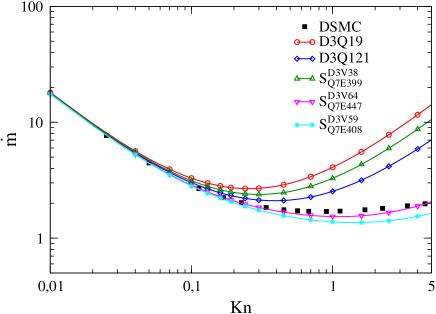
Figure 4: (Color online) Mass flow rate for common LB models and some exclusive ${\cal S}_{1}$ bulk flow models ($\Lambda_{\mathrm{index}}=0$).

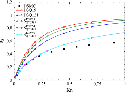
Figure 5: (Color online) Slip velocity for common LB models and some exclusive ${\cal S}_{1}$ bulk flow models ($\Lambda_{\mathrm{index}}=0$).

VI.1 Using discrete velocity models for bulk flow with $\Lambda_{\mathrm{index}}=0$

Figures 4 and 5 show the mass flow rate and the slip velocity at the wall for two known LB models, $D3Q19$ and $D3Q121$, and some new models of set ${\cal S}_{1}$ compared with DSMC data. For small $K\hskip-1.49994ptn$ the $D3Q19$ model (accuracy order $Q=5$) and the $D3Q121$ model (accuracy order $Q=9$) agree very well with the reference data. However, for higher $K\hskip-1.49994ptn$ both models exhibit strong deviations from the DSMC results. Similarly, the new model $S^{D3V38}_{Q7E399}$ with an accuracy order $Q=7$ and a minimal number of $38$ velocities fails for higher $K\hskip-1.49994ptn$. Although the high-order models $D3Q121$ and $S^{D3V38}_{Q7E399}$ recover flow regimes beyond the Navier-Stokes level (for a detailed discussion see Sect. III) the results remain unsatisfactory for finite $K\hskip-1.49994ptn$.

The new LB models of set ${\cal S}_{1}$ are of Gaussian quadrature order $Q=7$ and thus able to recover the momentum dynamics for small $M\hskip-1.49994pta$ up to the $4$th flow regime ($\Delta\Pi^{(4)}_{ij}=\mathcal{O}(M\hskip-1.49994pta^{2})$). If we analyze these models we observe for finite $K\hskip-1.49994ptn$, nevertheless, quite different results and considerable deviations from the DSMC results for both the mass flow rate and the slip velocity. The Gaussian quadrature order $Q$ is very important to recover high-order flow regimes, but not sufficient to guarantee accurate results of a LB model for finite $K\hskip-1.49994ptn$. This is also found for high-order LB models in $D=2$ dimensions 1.10 .

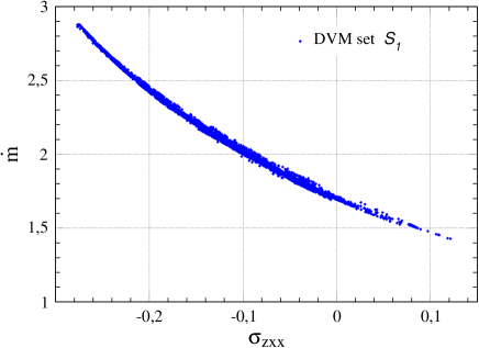
Figure 6: (Color online) Correlation between $\sigma_{zxx}$ and $\dot{m}$ for $K\hskip-1.49994ptn=0.4514$. Every dot represents a DVM within ${\cal S}_{1}$.

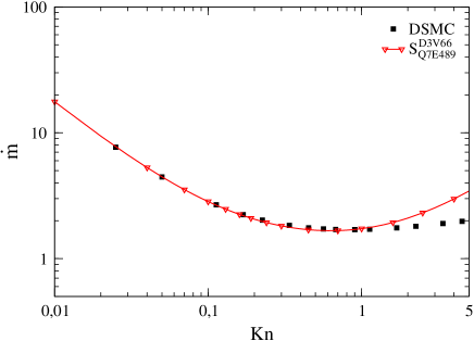
Figure 7: (Color online) Mass flow of the model $S^{D3V66}_{Q7E489}$ with the smallest error $|\sigma_{zxx}|$ within the set ${\cal S}_{1}$.

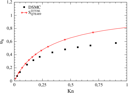
Figure 8: (Color online) Slip velocity of the model $S^{D3V66}_{Q7E489}$ with the smallest error $|\sigma_{zxx}|$ within the set ${\cal S}_{1}$.

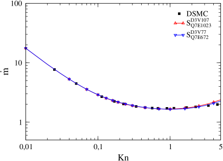
Figure 9: (Color online) Mass flow rate of selected ${\cal S}_{3}$ models ($\Lambda_{\mathrm{index}}=16$).

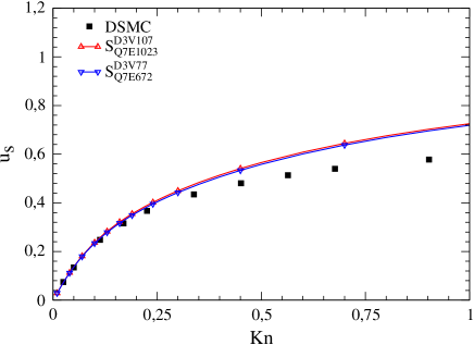
Figure 10: (Color online) Slip velocity of selected ${\cal S}_{3}$ models ($\Lambda_{\mathrm{index}}=16$).

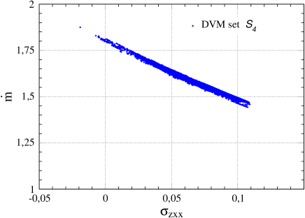
Figure 11: (Color online) Correlation between $\sigma_{zxx}$ and $\dot{m}$ for $K\hskip-1.49994ptn=0.4514$. Every dot represents a DVM within ${\cal S}_{4}$.

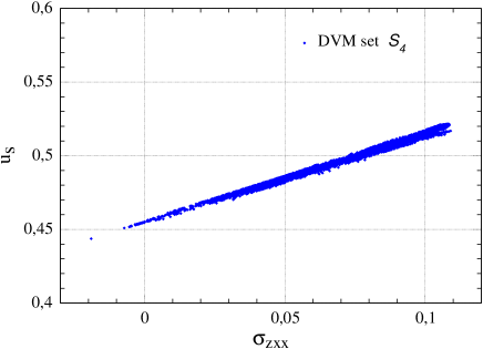
Figure 12: (Color online) Correlation between $\sigma_{zxx}$ and $u_{s}$ for $K\hskip-1.49994ptn=0.4514$. Every dot represents a DVM within ${\cal S}_{4}$.

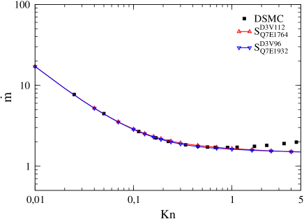
Figure 13: (Color online) Mass flow rate of selected ${\cal S}_{4}$ models ($\Lambda_{\mathrm{index}}=6245$).

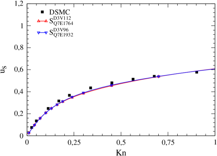
Figure 14: (Color online) Slip velocity of selected ${\cal S}_{4}$ models ($\Lambda_{\mathrm{index}}=6245$).

The reason for the failure of many high-order LB models for finite $K\hskip-1.49994ptn$ is their weak ability to recover the diffuse Maxwell boundary condition exactly. We assess this ability by considering the errors of the wall moments in Table 2. The exact definition of the models listed here can be found in Appendix 5. We here identified DVMs of the set ${\cal S}_{1}$ with wall moment errors as small as possible which thus ensure a good realization of the diffuse Maxwell boundary condition. For the two different models $S^{D3V64}_{Q7E447}$ and $S^{D3V59}_{Q7E408}$ some wall moment errors are given in Table 2 and the flow results are shown in Figs. 4 and 5. Due to smaller wall moment errors we observe for both models a significantly higher accuracy for finite $K\hskip-1.49994ptn$. The errors in the slip velocity are nearly the same whereas the predicted mass flow rate of the model $S^{D3V64}_{Q7E447}$ is more accurate. By using the CE analysis (see Sect. III) one can show that the relevant low $M\hskip-1.49994pta$ contributions to the momentum dynamics up to the Super-Burnett flow regime are affected by the third and fifth equilibrium moments. Therefore the higher accuracy of model $S^{D3V64}_{Q7E447}$ in the mass flow prediction is caused by a more accurate representation of the third wall moment $W_{zxx}$ (see Table 2).

DVM	Q	$\sigma$	$\sigma_{z}$	$\sigma_{xx}$	$\sigma_{zxx}$	$\sigma_{\Sigma}$
$D3Q19$	5	$-0.6667$	$-0.2764$	$-0.6667$	$-0.2764$	$0.5506$
$D3Q121$	9	$-0.4767$	$-0.1292$	$-0.4767$	$-0.1292$	$0.3685$
$S^{D3V38}_{Q7E399}$	7	$-0.4902$	$-0.1505$	$-0.5926$	$-0.2109$	$0.4042$
$S^{D3V64}_{Q7E447}$	7	$-0.0443$	$-0.0750$	$-0.1212$	$-0.0258$	$0.0621$
$S^{D3V59}_{Q7E408}$	7	$-0.0367$	$0.0932$	$-0.0794$	$0.0658$	$0.0576$
$S^{D3V66}_{Q7E489}$	7	$-0.3757$	$-0.0805$	$-0.2681$	$-0.0001$	$0.2720$

Table 2: Wall moment errors of standard LB model $D3Q19$, the common DVM $S_{Q9E594}^{D3V121}$ also known as $D3Q121$, as well as some exclusive ${\cal S}_{1}$ bulk flow models. $Q$ is the quadrature order.

If we consider the influence of the wall moment error $\sigma_{zxx}$ on the mass flow rate within all ${\cal S}_{1}$ models we observe a strong correlation between $\sigma_{zxx}$ and $\dot{m}$. This is shown in Fig. 6 for a Knudsen number of $K\hskip-1.49994ptn=0.4514$. Pearson’s linear correlation coefficient yields the value $-0.98$, exceeding in magnitude all other correlations of $\dot{m}$. It is interesting to notice that all models with a nearly vanishing wall moment error $\sigma_{zxx}$ predict a mass flow rate which is very close to the DSMC results of $\dot{m}_{DSMC}=1.76$ for $K\hskip-1.49994ptn=0.4514$. The LB model with the smallest error $|\sigma_{zxx}|$ within the set ${\cal S}_{1}$ is the $S^{D3V66}_{Q7E489}$ model. The wall moment errors are specified in Table 2. As a consequence of the minimal $|\sigma_{zxx}|$ error the mass flow rate is in excellent agreement with the DSMC results up to a Knudsen number of $K\hskip-1.49994ptn\approx 1$ (see Fig. 7). On the other hand the slip velocity, shown in Fig. 8, is less accurate compared to the other selected models ($S^{D3V64}_{Q7E447}$, $S^{D3V59}_{Q7E408}$) due to remaining inaccuracies of other wall moments.

These results confirm that a reliable LB model for finite $K\hskip-1.49994ptn$ flows requires both a high quadrature order $Q$ and small wall moment errors which guarantees a precise realization of the diffuse Maxwell boundary condition.

VI.2 Using discrete velocity models for wall-bounded flow with $\Lambda_{\mathrm{index}}=16$

In this section we discuss the set ${\cal S}_{3}$ of DVMs. These models are of Gaussian order $Q=7$ and include a wall moment constraint which ensures that the $\sigma_{zxx}$ error vanishes. Consequently, the wall accuracy index has the value $\Lambda_{\mathrm{index}}=16$, see Eq. (85). From this set of models we select the $S^{D3V107}_{Q7E1023}$ and $S^{D3V77}_{Q7E672}$ models which additionally have a small overall wall moment error $\sigma_{\Sigma}$ (see Table 3). The results for the mass flow rate, shown in Fig. 9, are in excellent agreement with the DSMC results due to the wall constraint $\sigma_{zxx}=0$. Additionally, the Knudsen minimum at $K\hskip-1.49994ptn\approx 1$ is very well reproduced. For the slip velocity (Fig. 10) we observe slight differences to the reference data which may be caused by remaining inaccuracies of other wall moments.

LB model	Q	$\sigma$	$\sigma_{z}$	$\sigma_{xx}$	$\sigma_{zxx}$	$\sigma_{zzzxx}$	$\sigma_{xxzzzzz}$	$\sigma_{\Sigma}$
$S^{D3V107}_{Q7E1023}$	7	$-0.0998$	$0.0247$	$-0.1482$	$0.0$	$0.0027$	$-0.0083$	$0.0849$
$S^{D3V77}_{Q7E672}$	7	$-0.0816$	$0.0343$	$-0.1339$	$0.0$	$0.0132$	$-0.0710$	$0.0765$

Table 3: Wall moment errors of some exclusive ${\cal S}_{3}$ models, where $Q$ is the quadrature order.

VI.3 Using discrete velocity models for wall-bounded flow with $\Lambda_{\mathrm{index}}=6245$

Another set of wall moment LB models, ${\cal S}_{4}$, is characterized by a Gaussian quadrature order $Q=7$ and scattering stencils which guarantee that all even wall moments up to the quadrature order $Q=7$ are represented exactly,

$$\sigma=\sigma_{i_{1}i_{2}}=\sigma_{i_{1}\dots i_{4}}=\sigma_{i_{1}\dots i_{6}}=0.$$ (115)

Consequently, the wall accuracy index has the value $\Lambda_{\mathrm{index}}=6245$, see Eq. (90). Similar to the model sets ${\cal S}_{1}$ and ${\cal S}_{3}$ discussed previously, we observe for ${\cal S}_{4}$ models a strong correlation between the wall moment $W_{zxx}$ and the flow results as well. Figure 11 shows the correlation between $\sigma_{zxx}$ and the mass flow and Fig. 12 shows the correlation between $\sigma_{zxx}$ and the slip velocity. Because of the strengths of these correlations we select the models $S^{D3V112}_{Q7E1764}$ and $S^{D3V96}_{Q7E1932}$ with small errors $|\sigma_{zxx}|$ (see Table 4). The Poiseuille flow results for these models are shown in Figs. 13 and 14. Both the mass flow rate and the slip velocity at the wall are in excellent agreement with the DSMC results up to $K\hskip-1.49994ptn=1$. The crucial point for the success of these models are very low errors for all wall moments up to the quadrature order ($Q=7$). However these models cannot predict the Knudsen minimum which was reproduced by models of groups ${\cal S}_{1}$ and ${\cal S}_{3}$.

LB model	Q	$\sigma$	$\sigma_{z}$	$\sigma_{xx}$	$\sigma_{zxx}$	$\sigma_{\Sigma}$
$S^{D3V112}_{Q7E1764}$	7	$0.0$	$0.0373$	$0.0$	$0.000005$	$0.0090$
$S^{D3V96}_{Q7E1932}$	7	$0.0$	$0.0386$	$0.0$	$0.0114$	$0.0101$

Table 4: Wall moment errors of some exclusive ${\cal S}_{4}$ models, where $Q$ is the quadrature order.

VI.4 Velocity profiles

Figs. 15 - 25 show the streamwise velocities of the considered LB models for several Knudsen numbers. At $K\hskip-1.49994ptn=0.05$ all models agree well with the DSMC results, however $D3Q19$ and $S^{D3V38}_{Q7E399}$ slightly over-predict the slip velocity at the walls. For higher $K\hskip-1.49994ptn$ the models $D3Q19$, $D3Q121$ and $S^{D3V38}_{Q7E399}$ no longer perform well due to errors of the wall moments. On the other hand, the models $S^{D3V64}_{Q7E447}$, $S^{D3V77}_{Q7E672}$ and $S^{D3V96}_{Q7E1932}$ show a significantly better prediction of the velocity field because of more accurate wall moments yielding a more precise realization of the diffuse Maxwell boundary condition.

In particular, the $S^{D3V96}_{Q7E1932}$ model guarantees a high accuracy for all wall moments up to the Gaussian quadrature order $Q=7$ and therefore remains quantitatively accurate at least up to $K\hskip-1.49994ptn\approx 1$. Only for Knudsen numbers higher than $K\hskip-1.49994ptn=2$ we observe a slight overestimation of the slip velocity.

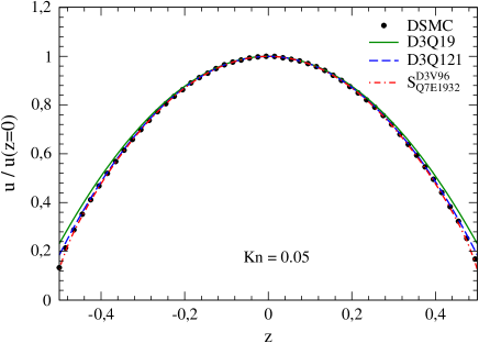
Figure 15: (Color online) Streamwise velocity profile for $K\hskip-1.49994ptn=0.05$.

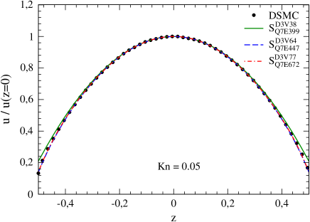
Figure 16: (Color online) Streamwise velocity profile for $K\hskip-1.49994ptn=0.05$.

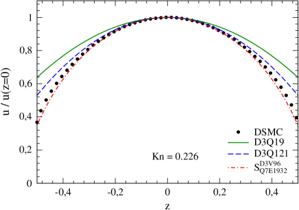
Figure 17: (Color online) Streamwise velocity profile for $K\hskip-1.49994ptn=0.226$.

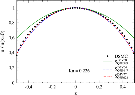
Figure 18: (Color online) Streamwise velocity profile for $K\hskip-1.49994ptn=0.226$.

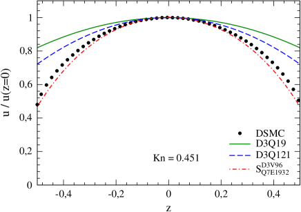
Figure 19: (Color online) Streamwise velocity profile for $K\hskip-1.49994ptn=0.451$.

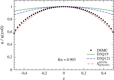
Figure 20: (Color online) Streamwise velocity profile for $K\hskip-1.49994ptn=0.903$.

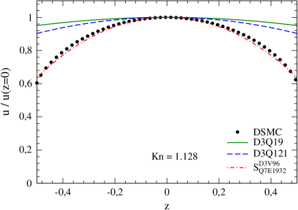
Figure 21: (Color online) Streamwise velocity profile for $K\hskip-1.49994ptn=1.128$.

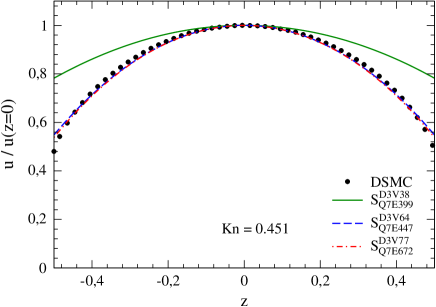
Figure 22: (Color online) Streamwise velocity profile for $K\hskip-1.49994ptn=0.451$.

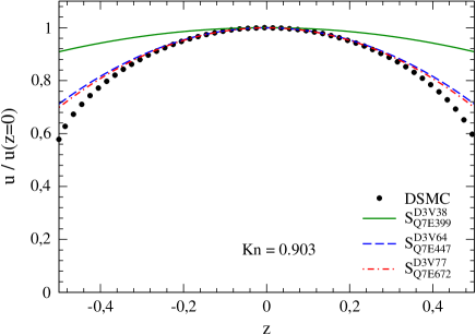
Figure 23: (Color online) Streamwise velocity profile for $K\hskip-1.49994ptn=0.903$.

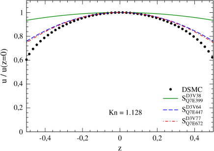
Figure 24: (Color online) Streamwise velocity profile for $K\hskip-1.49994ptn=1.128$.

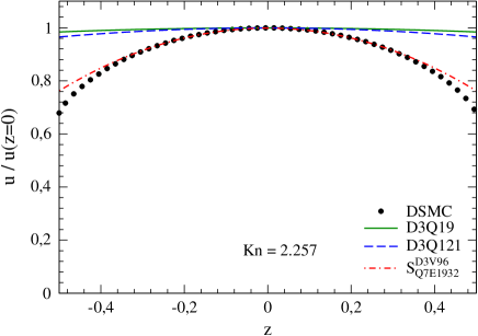
Figure 25: (Color online) Streamwise velocity profile for $K\hskip-1.49994ptn=2.257$.

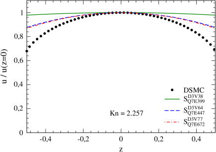
Figure 26: (Color online) Streamwise velocity profile for $K\hskip-1.49994ptn=2.257$.

VI.5 Knudsen layer

An even stronger requirement for the DVMs than correct evaluation of mass flow and slip velocity is to yield the correct velocity profile beyond the Navier–Stokes flow regime. For this purpose, we define for each solution $u(z)$ a quadratic velocity profile by

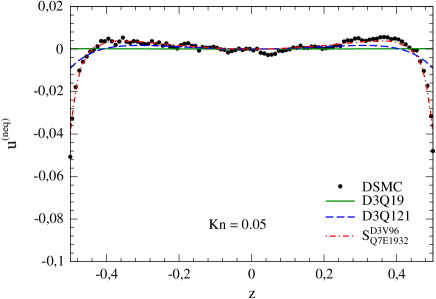
Figure 27: (Color online) Non-equilibrium velocity profile for $K\hskip-1.49994ptn=0.05$.

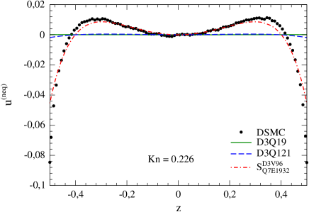
Figure 28: (Color online) Non-equilibrium velocity profile for $K\hskip-1.49994ptn=0.226$.

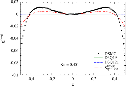
Figure 29: (Color online) Non-equilibrium velocity profile for $K\hskip-1.49994ptn=0.451$.

$$u^{(NS)}(z)=u(0)$$

$$\qquad\times\left(1-3\left(1-\frac{1}{l_{0}}\int_{-l_{0}/2}^{l_{0}/2}dz^{\prime}\>\frac{u(z^{\prime})}{u(0)}\right)\left(\frac{z}{l_{0}/2}\right)^{2}\right)$$ (116)

which gives the same mass flow as $u(z)$. The non-equilibrium content of $u(z)$ is measured by its deviation from the quadratic profile (VI.5),

$$u^{(neq)}(z)=u(z)-u^{(NS)}(z)\;.$$ (117)

Using the DSMC data for $u(z)$, we find a reference function $u^{(neq)}(z)$ for each $K\hskip-1.49994ptn$ number the DVMs compete with. As shown for $K\hskip-1.49994ptn=0.05$ in Fig. 27, the DSMC data show a small velocity defect at the vicinity of the wall—the Knudsen layer—such that $u^{(neq)}<0$. In turn, there is an exceed of non-equilibrium velocity in the bulk, $u^{(neq)}>0$, by definition of Eq. (VI.5). The standard model $D3Q19$ is not able to show a Knudsen layer, due to its low quadrature order, $Q=5$. It yields a strictly quadratic profile with $u^{(neq)}(z)=0$. The model $D3Q121$ with higher quadrature order, $Q=9$, shows some velocity defect, however, it does not quite match the DSMC result for its wall moments are inaccurate. On the other hand, the DVM $S_{Q7E1932}^{D3V96}$, which has both a high quadrature order and (almost) correct wall moments, shows excellent agreement with DSMC data in the Knudsen layer for $K\hskip-1.49994ptn=0.05$.

This hierarchy of DVMs remains for higher $K\hskip-1.49994ptn$ numbers. For $K\hskip-1.49994ptn=0.226$, the Knudsen layer is more pronounced, see Fig. 28. While the models $D3Q19$ and $D3Q121$ are unsatisfactory, the model $S_{Q7E1932}^{D3V96}$ is able to describe the Knudsen layer. Increasing the $K\hskip-1.49994ptn$ number further high-order flow regimes gain more importance, causing the DVMs presented here to cease to be valid for evaluating the non-equilibrium velocity profile. This is exemplified for $K\hskip-1.49994ptn=0.451$ in Fig. 29.

VII Conclusion

In this paper we presented high-order Lattice–Boltzmann (LB) models for solving the Boltzmann–BGK equation for finite $K\hskip-1.49994ptn$ number flows.

It was shown how to derive new discrete velocity models (DVMs) for any quadrature order using an efficient algorithm. The energy of a stencil was bounded from above in order to be able to define complete sets of minimal DVMs. These sets comprise more than $50000$ models with $7$th quadrature order in $D=3$ spatial dimensions. In future investigations, the collection of minimal discrete velocity models for high-order LB simulations can be systematically extended.

We analytically derived a theorem via the Chapman–Enskog expansion which enables us to identify the recovered flow regimes of any LB model, i.e. Navier–Stokes, Burnett, Super–Burnett, and so on. For isothermal flows, this theorem rigorously relates the velocity space discretization error of a velocity moment for low $M\hskip-1.49994pta$ values with the quadrature order $Q$ of a LB model. Thus, one can tell from the quadrature order $Q$ which flow regime is exactly recovered by the LB model for $M\hskip-1.49994pta\to 0$. In particular, it was shown for isothermal flows that even the standard models with $Q=5$ recover the Burnett momentum dynamics for $M\hskip-1.49994pta\to 0$. The $7$th order LB models we focused on here recover the momentum flux tensor of non-equilibrium gas flows up to the $4$th flow regime for $M\hskip-1.49994pta\to 0$.

Aside from non-equilibrium effects in the bulk, wall-bounded high $K\hskip-1.49994ptn$ number flows require a LB model to correctly describe the gas-surface interaction. We observed that several high-order LB models show significant deviations from reference results because of their poor ability to recover the diffuse Maxwell boundary condition accurately. In order to characterize this capability we defined an analytical criterion for a DVM for the exact implementation of the diffuse Maxwell boundary condition. It was shown how to generate in a systematic way high-order DVMs with the inherent ability to fulfill the diffuse Maxwell boundary condition. Alternatively, it is possible to arrive at discrete velocity models which obey the criterion for even velocity moments at the wall by simply using scattering stencils. The wall accuracy index $\Lambda_{\mathrm{index}}$ was put forward to label the velocity moments at the wall evaluated correctly by a discrete velocity model. The $7$th order model $S_{Q7E1932}^{D3V96}$, e.g., was found with a wall accuracy index $\Lambda_{\mathrm{index}}=6245$ and an almost exact representation of the wall moments up to the $7$th order. The circumstance that models with even numbers of discrete velocities perform better than for odd numbers can be due to the low net weight of erroneous wall-parallel (and zero) velocities in half-space quadratures. For an exact integration of particle velocities emitted by the wall, we derived a sufficient condition on the wall accuracy order $\Lambda$.

At finite $K\hskip-1.49994ptn$, we compared our Poiseuille flow LB results with those of DSMC. We found the agreement is strongly correlated with the wall criterion on the one hand and requires the use of high-order DVMs ($Q\geq 7$) on the other. Therefore, the correct evaluation of high $K\hskip-1.49994ptn$ number Poiseuille flow requires both, a sufficiently high quadrature order and an exact representation of the diffuse Maxwell boundary condition. Consequently, the model $S_{Q7E1932}^{D3V96}$ yields an excellent agreement with DSMC for both the mass flow and the slip velocity, using $K\hskip-1.49994ptn$ numbers up to $K\hskip-1.49994ptn\simeq 1$. In the velocity profiles one can clearly recognize that the discrete velocity model $S_{Q7E1932}^{D3V96}$ recovers the Knudsen layer in the vicinity of the wall for $K\hskip-1.49994ptn\lesssim 0.3$, while standard discrete velocity models utterly fail. Thus we recommend using $S_{Q7E1932}^{D3V96}$ for finite $K\hskip-1.49994ptn$ number flows.

For $K\hskip-1.49994ptn\gtrsim 0.3$, the results for the non-equilibrium velocity profile departs from the DSMC results, because the flow regimes are only recovered up to the $4$th Chapman–Enskog level and there are remaining errors in high-order wall moments. However, we expect that for LB models with a sufficiently high quadrature order and wall accuracy order, a more precise representation of the Knudsen layer phenomenon can be obtained. This will be part of our future investigations. Moreover, it remains to be seen whether the Knudsen layer turns out to be a nonperturbative phenomenon in the sense of the Chapman–Enskog expansion.

Appendix A Three-dimensional DVMs

Here we present DVMs generated by the algorithm shown in Sect. II and used in the introductory example and the numerical test case in Sect. VI. The stencil’s symbol is explained in Eq. (24), $c$ is the lattice speed, $g$ counts the stencil groups $S_{g}$ generated by the symmetries of the lattice from a single velocity $\boldsymbol{\mathbf{\xi}}^{(g)}$ yielding $V_{g}$ velocities. Each velocity in $S_{g}$ is weighted by $\overline{\mathrm{w}}_{g}$, see Eq. (18), when using the quadrature prescription (10).

$\boldsymbol{S_{Q5E24}^{D3V15}}$		$c=1.2247448713915890$
g	$\boldsymbol{\mathbf{\xi}}^{(g)}/c$	$V_{g}$	$\overline{\mathrm{w}}_{g}$
1	(0,0,0)	1	3.8888888888888889e-1
2	(2,0,0)	6	2.7777777777777778e-2
3	(1,1,-1)	8	5.5555555555555556e-2

Table 5: DVM used for the introductory example.

$\boldsymbol{S_{Q7E399}^{D3V38}}$		$c=0.75000000000000000$
g	$\boldsymbol{\mathbf{\xi}}^{(g)}/c$	$V_{g}$	$\overline{\mathrm{w}}_{g}$
1	(1,0,0)	6	7.2239858906525573e-2
2	(4,0,0)	6	6.3648834019204390e-3
3	(2,2,0)	12	4.3895747599451303e-2
4	(6,0,0)	6	4.1805473904239336e-5
5	(4,4,4)	8	1.7146776406035665e-4

Table 6: DVM with minimal velocity count within the set ${\cal S}_{1}$.

$\boldsymbol{S_{Q7E219}^{D3V38}}$		$c=0.86602540378443865$
g	$\boldsymbol{\mathbf{\xi}}^{(g)}/c$	$V_{g}$	$\overline{\mathrm{w}}_{g}$
1	(1,0,0)	6	6.7724867724867725e-2
2	(2,0,0)	6	5.5555555555555556e-2
3	(2,2,2)	8	4.6296296296296296e-3
4	(2,2,0)	12	1.8518518518518519e-2
5	(6,0,0)	6	1.7636684303350970e-4

Table 7: DVM with minimal velocity count within the set ${\cal S}_{1}$.

$\boldsymbol{S_{Q7E408}^{D3V59}}$		$c=0.74685634388439233$
g	$\boldsymbol{\mathbf{\xi}}^{(g)}/c$	$V_{g}$	$\overline{\mathrm{w}}_{g}$
1	(0,0,0)	1	2.0080700829205231e-2
2	(1,1,1)	8	8.9344539381631413e-2
3	(4,0,0)	6	1.8287317703258027e-3
4	(3,3,3)	8	5.2273139486813077e-4
5	(3,3,0)	12	2.3272910797607214e-3
6	(3,1,1)	24	9.2533853908214560e-3

Table 8: Selection of DVMs within the set ${\cal S}_{1}$. See Sect. VI for a discussion.

$\boldsymbol{S_{Q7E447}^{D3V64}}$		$c=0.69965342816864754$
g	$\boldsymbol{\mathbf{\xi}}^{(g)}/c$	$V_{g}$	$\overline{\mathrm{w}}_{g}$
1	(2,0,0)	6	5.9646397884737016e-3
2	(1,1,1)	8	8.0827437008387392e-2
3	(5,0,0)	6	1.1345266793939999e-3
4	(3,3,3)	8	9.5680047874015889e-4
5	(3,3,0)	12	3.9787631334632013e-3
6	(3,1,1)	24	1.0641080987258957e-2

Table 9: Selection of DVMs within the set ${\cal S}_{1}$. See Sect. VI for a discussion.

$\boldsymbol{S_{Q7E489}^{D3V66}}$		$c=0.91181414856781201$
g	$\boldsymbol{\mathbf{\xi}}^{(g)}/c$	$V_{g}$	$\overline{\mathrm{w}}_{g}$
1	(1,0,0)	6	8.5874589554625067e-2
2	(3,0,0)	6	7.7875559017476937e-3
3	(2,2,0)	12	1.1890500729870710e-4
4	(2,1,1)	24	1.8125533818334885e-2
5	(7,0,0)	6	2.7809545430205753e-6
6	(4,4,0)	12	1.3089748390696516e-4

Table 10: Selection of DVMs within the set ${\cal S}_{1}$. See Sect. VI for a discussion.

$\boldsymbol{S_{Q9E471}^{D3V79}}$		$c=1.0000000000000000$
g	$\boldsymbol{\mathbf{\xi}}^{(g)}/c$	$V_{g}$	$\overline{\mathrm{w}}_{g}$
1	(0,0,0)	1	1.0570987654320988e-1
2	(1,0,0)	6	3.8095238095238095e-2
3	(2,0,0)	6	2.8645833333333333e-2
4	(1,1,1)	8	4.9479166666666667e-2
5	(2,2,2)	8	5.2083333333333333e-4
6	(2,2,0)	12	5.2083333333333333e-3
7	(6,0,0)	6	2.7557319223985891e-6
8	(3,3,3)	8	9.6450617283950617e-6
9	(3,1,1)	24	1.3020833333333333e-3

Table 11: DVM with minimal velocity count within the set ${\cal S}_{2}$. For a description of the symbols, see Tab. 6.

$\boldsymbol{S_{Q9E594}^{D3V121}}$		$c=1.1969797703930744$
g	$\boldsymbol{\mathbf{\xi}}^{(g)}/c$	$V_{g}$	$\overline{\mathrm{w}}_{g}$
1	(0,0,0)	1	3.0591622029486006e-2
2	(0,0,-1)	6	9.8515951037263392e-2
3	(1,1,-1)	8	2.7525005325638124e-2
4	(0,0,-3)	6	3.2474752708807381e-4
5	(2,2,-2)	8	1.8102175157637424e-4
6	(2,0,-2)	12	4.2818359368108407e-4
7	(1,0,-2)	24	6.1110233668334243e-3
8	(3,3,-3)	8	6.9287508963860285e-7
9	(1,1,-3)	24	1.0683400245939109e-4
10	(2,0,-3)	24	1.4318624115480294e-5

Table 12: Common DVM ($D3Q121$ Meng ) within the set ${\cal S}_{2}$. For a description of the symbols, see Tab. 6.

$\boldsymbol{S_{Q7E672}^{D3V77}}$		$c=0.62590566441325041$
g	$\boldsymbol{\mathbf{\xi}}^{(g)}/c$	$V_{g}$	$\overline{\mathrm{w}}_{g}$
1	(2,0,0)	6	6.5178619315224175e-3
2	(1,1,1)	8	5.8638132347907334e-2
3	(6,0,0)	6	1.0066312290789269e-3
4	(3,3,3)	8	2.1962967289288607e-3
5	(3,3,0)	12	4.8042518606023833e-3
6	(3,1,1)	24	1.5528601406828448e-2
7	(0,0,0)	1	2.9560614762917757e-2
8	(4,4,0)	12	6.8996146397277359e-4

Table 13: Selection of DVMs within the set ${\cal S}_{3}$. See Sect. IV.3 for a discussion.

$\boldsymbol{S_{Q7E1023}^{D3V107}}$		$c=0.61887631323925978$
g	$\boldsymbol{\mathbf{\xi}}^{(g)}/c$	$V_{g}$	$\overline{\mathrm{w}}_{g}$
1	(1,1,1)	8	5.4242093013777495e-2
2	(2,1,0)	24	2.4637212114133877e-3
3	(5,0,0)	6	1.5469959015615954e-3
4	(3,3,3)	8	1.9425678925800591e-3
5	(3,3,0)	12	7.2337497640759286e-3
6	(3,1,1)	24	1.4384326790070621e-2
7	(0,0,0)	1	4.4998866720663948e-2
8	(6,2,2)	24	2.1182172560744541e-4

Table 14: Selection of DVMs within the set ${\cal S}_{3}$. See Sect. IV.3 for a discussion.

$\boldsymbol{S_{Q7E1932}^{D3V96}}$		$c=0.37787639086813054$
g	$\boldsymbol{\mathbf{\xi}}^{(g)}/c$	$V_{g}$	$\overline{\mathrm{w}}_{g}$
1	(1,1,1)	8	1.2655649299880090e-3
2	(3,3,3)	8	2.0050978770655310e-2
3	(3,1,1)	24	2.7543347614356814e-2
4	(4,4,4)	8	4.9712543563172566e-3
5	(7,1,1)	24	3.6439016726158895e-3
6	(6,6,1)	24	1.7168180273737716e-3

Table 15: Selection of DVMs within the set ${\cal S}_{4}$. See Sect. IV.3 for a discussion.

$\boldsymbol{S_{Q7E1764}^{D3V112}}$		$c=0.40531852273291520$
g	$\boldsymbol{\mathbf{\xi}}^{(g)}/c$	$V_{g}$	$\overline{\mathrm{w}}_{g}$
1	(1,1,1)	8	3.3503407500643648e-3
2	(3,1,1)	24	2.8894128958152456e-2
3	(4,4,4)	8	4.5930345162087793e-3
4	(3,2,2)	24	4.4163148398082762e-3
5	(7,1,1)	24	2.3237070220062610e-3
6	(5,5,1)	24	3.3847240912752922e-3

Table 16: Selection of DVMs within the set ${\cal S}_{4}$. See Sect. IV.3 for a discussion.

Appendix B Two-dimensional DVMs

In this Appendix, we present minimal DVMs for $D=2$. As shown in Tab. 1 above, there are three sets of DVMs concerned with $D=2$. The $y$ component is absent. For all but the wall accuracy index $\Lambda_{\mathrm{index}}$, the definitions are the same as for $D=3$. Since there are no $y$ components of wall moments, we have to set $m_{y}=0$ in Eq. (IV.3). The wall accuracy index is then defined as before, see Eq. (83), but there are only $L=14$ components in the vector

$${\bf T}^{\alpha} = (1,\>\xi_{\alpha z},\>\xi_{\alpha x}^{2},\>\xi_{\alpha z}^{3},\>\xi_{\alpha z}\xi_{\alpha x}^{2},\>\xi_{\alpha x}^{4},\>$$ (118)

$$\>\xi_{\alpha z}^{5},\>\xi_{\alpha z}^{3}\xi_{\alpha x}^{2},\>\xi_{\alpha z}\xi_{\alpha x}^{4},\>\xi_{\alpha x}^{6},\>$$

$$\>\xi_{\alpha z}^{7},\>\xi_{\alpha z}^{5}\xi_{\alpha x}^{2},\>\xi_{\alpha z}^{3}\xi_{\alpha x}^{4},\xi_{\alpha z}\xi_{\alpha x}^{6})\;,$$

whereas $b_{k}$ are the components of the vector

$${\bf b} = (W,\>W_{z},\>W_{xx},\>W_{zzz},\>W_{zxx},\>W_{xxxx},\>W_{zzzzz},\>$$ (119)

$$\>W_{zzzxx},\>W_{zxxxx},\>W_{xxxxxx},\>W_{zzzzzzz},\>$$

$$\>W_{zzzzzxx},\>W_{zzzxxxx},\>W_{zxxxxxx})\;,$$

cf. Eqs. (78) and (79).

The set ${\cal S}_{5}$ comprises all $1188$ minimal DVMs with quadrature order $Q=7$ in the energy sphere given by $E\leq 250$. These are discrete velocity models for bulk flow, i.e. the wall accuracy index $\Lambda_{\mathrm{index}}$ is zero. The DVM with lowest velocity count $V_{min}=16$ is $S_{Q7E58}^{D2V16}$ and it is shown in Tab. 17. Increasing the quadrature order to $Q=9$, we find $592$ DVMs in the set ${\cal S}_{6}$ where $E_{max}=300$. The DVM with the lowest velocity count in ${\cal S}_{6}$ is $S_{Q7E944}^{D2V32}$, see Tab. 18, and it yields $V=33$. Finally, we identified $21952$ DVMs with quadrature order $Q=7$ which have scattering stencils, i.e. their wall accuracy index is $\Lambda_{\mathrm{index}}=549$. The stencil energy is bounded for these models by $E_{max}=1000$ to define the set ${\cal S}_{7}$. The DVM with the lowest velocity count gives $V_{min}=20$. Optimizing for both $\sigma_{zx}$ and $\sigma_{\Sigma}$ yields the DVM $S_{Q7E944}^{D2V32}$ shown in Tab. 19. The latter is expected to give back excellent results for planar Poiseuille flow.

$\boldsymbol{S_{Q7E58}^{D2V16}}$		$c=0.86602540378443865$
g	$\boldsymbol{\mathbf{\xi}}^{(g)}/c$	$V_{g}$	$\overline{\mathrm{w}}_{g}$
1	(1,0)	4	1.5802469135802469e-1
2	(2,0)	4	6.1728395061728395e-2
3	(2,2)	4	2.7777777777777778e-2
4	(4,0)	4	2.4691358024691358e-3

Table 17: DVM with the lowest velocity count $V_{min}=16$ in the set ${\cal S}_{5}$ where $D=2$, $Q=7$, and $E\leq 250$ (see Tab. 1).

$\boldsymbol{S_{Q9E132}^{D2V33}}$		$c=1.1587791906520175$
g	$\boldsymbol{\mathbf{\xi}}^{(g)}/c$	$V_{g}$	$\overline{\mathrm{w}}_{g}$
1	(0,0)	1	1.6198651186147246e-1
2	(1,0)	4	1.4320396528198750e-1
3	(1,1)	4	3.3883996404301766e-2
4	(2,0)	4	5.5611157082744134e-3
5	(2,2)	4	8.4479885070276616e-5
6	(3,0)	4	1.1325437650467775e-3
7	(2,1)	8	1.2816907733721003e-2
8	(4,4)	4	3.4555225091487045e-6

Table 18: DVM with the lowest velocity count $V_{min}=33$ in the set ${\cal S}_{6}$ where $D=2$, $Q=9$, and $E\leq 300$ (see Tab. 1).

$\boldsymbol{S_{Q7E944}^{D2V32}}$		$c=0.34040702226615838$
g	$\boldsymbol{\mathbf{\xi}}^{(g)}/c$	$V_{g}$	$\overline{\mathrm{w}}_{g}$
1	(1,1)	4	8.4201053650845727e-2
2	(2,2)	4	5.0708714918479963e-2
3	(5,1)	8	4.4541157350549509e-2
4	(6,4)	8	1.2646044225450934e-2
5	(12,3)	8	3.5791413933671213e-4

Table 19: DVM with optimal values for the wall errors in the set ${\cal S}_{7}$ where $D=2$, $Q=7$, $E\leq 1000$, and $\sigma_{i_{1}\dots i_{2n}}=0$. (see Tab. 1).

Appendix C Error estimate of equilibrium moments

For a detailed analysis of the quadrature error of an equilibrium moment $\Delta M^{(0)}_{i_{1}\dots i_{k}}$ we distinguish four different cases.

Case 1: $k\leq N$ and $k+N\leq Q$

The Hermite order $N$ is high enough to capture all contributions of the Hermite polynomials $\mathcal{H}^{(k)}_{i_{1}\dots i_{k}},\mathcal{H}^{(k-2)}_{i_{1}\dots i_{k-2}},\dots$ and the quadrature order guarantees an exact evaluation of all terms in Eq. (54). Thus the moment $M^{(0)}_{i_{1}\dots i_{k}}$ is exactly recovered and

$$\Delta M^{(0)}_{i_{1}\dots i_{k}}=0\;.$$ (120)

Case 2: $k\leq N$ and $k+N>Q$

Although the Hermite order is high enough, the quadrature order $Q=n_{0}+k$, with $n_{0}<N$, is not high enough to evaluate $M^{(0)}_{i_{1}\dots i_{k}}$ exactly. For low $M\hskip-1.49994pta$ values, the leading term of the quadrature error in Eq. (54) is the smallest value of $n$ exceeding $n_{0}$, due to the relation (52). This term is the one with $n=n_{0}+1$ in Eq. (54) and we can write

$$\Delta M^{(0)}_{i_{1}\dots i_{k}} =\frac{1}{(Q-k+1)!}a^{(0)}_{i_{1}\dots i_{Q-k+1}}\sum_{\alpha}\mathrm{w}_{\alpha}\mathcal{H}^{(Q-k+1)}_{i_{1}\dots i_{Q-k+1}}(\boldsymbol{\mathbf{\xi}}_{\alpha})\mathcal{H}^{(k)}_{i_{1}\dots i_{k}}(\boldsymbol{\mathbf{\xi}}_{\alpha})\quad+\textit{subleading terms}$$

$$=\mathcal{O}\left(M\hskip-1.49994pta^{Q-k+1}\right)\;,$$ (121)

where the subleading terms contain errors with a higher $M\hskip-1.49994pta$ power compared to the first term. Obviously, the quadrature error $\Delta M^{(0)}_{i_{1}\dots i_{k}}$ is finite for low $M\hskip-1.49994pta$ values, see Eq. (54). Consequently we obtain $\Delta M^{(0)}_{i_{1}\dots i_{k}}=\mathcal{O}\left(M\hskip-1.49994pta^{0}\right)$ for $Q-k+1<0$.

Case 3: $k>N$ and $k+N\leq Q$

The Hermite order $N$ is not high enough to capture the moment $M^{(0)}_{i_{1}\dots i_{k}}$ completely whereas the quadrature order guarantees the exact evaluation of all terms in Eq. (54). Therefore errors are produced by the absence of terms in the equilibrium function which are beyond the Hermite order $N$. The leading term in the quadrature error is thus $\sim a^{(0)}_{i_{1}\dots i_{N+1}}$ and with Eq. (52) we get

$$\Delta M^{(0)}_{i_{1}\dots i_{k}}=\mathcal{O}\left(M\hskip-1.49994pta^{N+1}\right).$$ (122)

Case 4: $k>N$ and $k+N>Q$

Neither the Hermite order $N$ is high enough to recover $M^{(0)}_{i_{1}\dots i_{k}}$ nor the quadrature order $Q$ guarantees an exact evaluation. The relevant quadrature error in the sense of the $M\hskip-1.49994pta$ expansion of the equilibrium function $f^{(0)}$ is determined analogously to case 2 by

$$\Delta M^{(0)}_{i_{1}\dots i_{k}}=\mathcal{O}\left(M\hskip-1.49994pta^{Q-k+1}\right)$$ (123)

for $Q-k+1\geq 0$ and $\Delta M^{(0)}_{i_{1}\dots i_{k}}=\mathcal{O}\left(M\hskip-1.49994pta^{0}\right)$ otherwise.

These cases can be summarized into a more compact relation

$$\Delta M^{(0)}_{i_{1}\dots i_{k}}=\begin{cases}0&\text{for }k+N\leq Q\text{ and }k\leq N\\ \mathcal{O}\left(M\hskip-1.49994pta^{N+1}\right)&\text{for }k+N\leq Q\text{ and }k>N\\ \mathcal{O}\left(M\hskip-1.49994pta^{Q-k+1}\right)&\text{for }k-1\leq Q<k+N\\ \mathcal{O}\left(M\hskip-1.49994pta^{0}\right)&\text{for }Q<k-1\;.\end{cases}$$ (124)

Appendix D Proof of the quadrature error theorem

The theorem in Sect. III.3 is proved by induction. Based on Eq. (III.3) the truncation error of $M^{(1)}_{i_{1}\dots i_{k}}$ is determined by

$$\Delta M^{(1)}_{i_{1}\dots i_{k}} =-\tau\left[\Delta\partial^{(0)}_{t}M^{(0)}_{i_{1}\dots i_{k}}+\partial_{j_{1}}\Delta M^{(0)}_{i_{1}\dots i_{k}j_{1}}\right].$$ (125)

Because of Eq. (III.3) the relevant error with respect to the $M\hskip-1.49994pta$ power is produced by the highest equilibrium moment which is contained in the second term on the right-hand side. The first term does not contribute to the dominant truncation error, because it consists of a lower equilibrium moment and the multiple-scale derivative $\partial^{(0)}_{t}$ does not change the $M\hskip-1.49994pta$ power of this error term. Consequently we find

$$\Delta M^{(1)}_{i_{1}\dots i_{k}} =-\tau\partial_{j_{1}}\Delta M^{(0)}_{i_{1}\dots i_{k}j_{1}}+\textit{subleading terms}$$ (126)

and with Eq. (III.3) the estimate

$$\Delta M^{(1)}_{i_{1}\dots i_{k}}=\begin{cases}0&\text{for }2(k+1)+1\leq Q\\ \mathcal{O}\left(M\hskip-1.49994pta^{Q-k}\right)&\text{for }k\leq Q<2(k+1)+1\\ \mathcal{O}\left(M\hskip-1.49994pta^{0}\right)&\text{for }Q<k\end{cases}\text{ .}$$ (127)

For the next CE moment we obtain from Eq. (III.3)

$$M^{(2)}_{i_{1}\dots i_{k}} =-\tau\left[\partial^{0}_{t}M^{(1)}_{i_{1}\dots i_{k}}-\frac{1}{\rho}\sum_{q}\frac{\partial M^{(0)}_{i_{1}\dots i_{k}}}{\partial(\partial_{j_{1}\dots j_{q}}^{(q)}u_{s})}\partial_{j_{1}\dots j_{q}}^{(q)}\left(\partial_{r}\Pi^{(1)}_{rs}\right)+\partial_{j}M^{(1)}_{i_{1}\dots i_{k}j}\right].$$ (128)

The error of the first term on the right-hand side is given by Eq. (127) where the time derivative $\partial_{t}^{(0)}$ does not affect the $M\hskip-1.49994pta$ power

$$\Delta\partial_{t}^{(0)}M^{(1)}_{i_{1}\dots i_{k}}=\partial_{t}^{(0)}\Delta M^{(1)}_{i_{1}\dots i_{k}}$$

$$\quad=\begin{cases}0&\text{for }2(k+1)+1\leq Q\\ \mathcal{O}\left(M\hskip-1.49994pta^{Q-k}\right)&\text{for }k\leq Q<2(k+1)+1\\ \mathcal{O}\left(M\hskip-1.49994pta^{0}\right)&\text{for }Q<k\end{cases}\text{ .}$$ (129)

With respect to Eq. (III.3) we get for the error of the next term

$$\Delta\frac{\partial M^{(0)}_{i_{1}\dots i_{k}}}{\partial(\partial_{j_{1}\dots j_{q}}^{(q)}u_{s})}=\begin{cases}0&\text{for }2k+1\leq Q\\ \mathcal{O}\left(M\hskip-1.49994pta^{Q-k}\right)&\text{for }k\leq Q<2k+1\\ \mathcal{O}\left(M\hskip-1.49994pta^{0}\right)&\text{for }Q<k\end{cases}$$ (130)

where we have to take into account that the $M\hskip-1.49994pta$ power of the error term is decreased by one by the derivative $\partial/\partial(\partial_{j_{1}\dots j_{q}}^{(q)}u_{s})$. Based on Eq. (127) we obtain

$$\Delta\Pi^{(1)}_{rs}=\begin{cases}0&\text{for }7\leq Q\\ \mathcal{O}\left(M\hskip-1.49994pta^{Q-2}\right)&\text{for }2\leq Q<7\\ \mathcal{O}\left(M\hskip-1.49994pta^{0}\right)&\text{for }Q<2\end{cases}$$ (131)

and for the last term in Eq. (128)

$$\Delta M^{(1)}_{i_{1}\dots i_{k}j}=\begin{cases}0&\text{for }2(k+2)+1\leq Q\\ \mathcal{O}\left(M\hskip-1.49994pta^{Q-k-1}\right)&\text{for }k+1\leq Q<2(k+2)+1\\ \mathcal{O}\left(M\hskip-1.49994pta^{0}\right)&\text{for }Q<k+1\end{cases}\text{ .}$$ (132)

Due to $k\geq 2$ the error estimate of all terms in Eq. (128) implies that the relevant quadrature error of $M^{(2)}_{i_{1}\dots i_{k}}$ is contained in the last term of Eq. (128) and thus we get

$$\Delta M^{(2)}_{i_{1}\dots i_{k}}=-\tau\partial_{j_{2}}\Delta M^{(1)}_{i_{1}\dots i_{k}j_{2}}+\textit{subleading terms}$$

$$\quad=(-\tau)^{2}\partial_{j_{1}}\partial_{j_{2}}\Delta M^{(0)}_{i_{1}\dots i_{k}j_{1}j_{2}}+\textit{subleading terms}.$$ (133)

In the last step of the proof we have to show the relation (61) for an integer $n$ assuming that the relation is valid for $n-1,n-2,\dots,1$. We analyze the error of all terms on the right-hand side of Eq. (III.3).

$$\Delta M^{(n)}_{i_{1}\dots i_{k}}=-\tau\left[\Delta\partial^{(0)}_{t}M^{(n-1)}_{i_{1}\dots i_{k}}-\Delta\left\{\frac{1}{\rho}\sum_{m=1}^{n-1}\sum_{q}\frac{\partial M^{(n-m-1)}_{i_{1}\dots i_{k}}}{\partial(\partial_{j_{1}\dots j_{q}}^{(q)}u_{s})}\partial_{j_{1}\dots j_{q}}^{(q)}\left(\partial_{r}\Pi^{(m)}_{rs}\right)\right\}+\partial_{j}\Delta M^{(n-1)}_{i_{1}\dots i_{k}j}\right].$$ (134)

Using Eq. (61) for $n-1$ we find

$$\Delta\partial_{t}^{(0)}M^{(n-1)}_{i_{1}\dots i_{k}} =\partial_{t}^{(0)}\Delta M^{(n-1)}_{i_{1}\dots i_{k}}=(-\tau)^{n-1}\partial_{t}^{(0)}\partial_{j_{1}}\dots\partial_{j_{n-1}}\Delta M^{(0)}_{i_{1}\dots i_{k}j_{1}\dots j_{n-1}}+\textit{subleading terms}$$

$$=\begin{cases}0&\text{for }2(k+n-1)+1\leq Q\\ \mathcal{O}\left(M\hskip-1.49994pta^{Q-k-n+2}\right)&\text{for }k+n-2\leq Q<2(k+n-1)+1\\ \mathcal{O}\left(M\hskip-1.49994pta^{0}\right)&\text{for }Q<k+n-2\end{cases}$$ (135)

where $\partial_{t}^{(0)}$ does not affect the $M\hskip-1.49994pta$ power of the error term. Furthermore, we can estimate the error of $\partial M^{(n-m-1)}_{i_{1}\dots i_{k}}/\partial(\partial_{j_{1}\dots j_{q}}^{(q)}u_{s})$ for $m=1,\dots,n-1$ by using Eq. (61) for $n-m-1$ in combination with Eq. (III.3)

$$\Delta\frac{\partial M^{(n-m-1)}_{i_{1}\dots i_{k}}}{\partial(\partial_{j_{1}\dots j_{q}}^{(q)}u_{s})}=\begin{cases}0&\text{for }2(k+n-m-1)+1\leq Q\\ \mathcal{O}\left(M\hskip-1.49994pta^{Q-k-n+m+1}\right)&\text{for }k+n-m-1\leq Q<2(k+n-m-1)+1\\ \mathcal{O}\left(M\hskip-1.49994pta^{0}\right)&\text{for }Q<k+n-m-1\end{cases}$$ (136)

where the derivatives $\partial/\partial(\partial_{j_{1}\dots j_{q}}^{(q)}u_{s})$ reduce the $M\hskip-1.49994pta$ power of the error term by one. The error of the quantity $\Pi^{(m)}_{rs}$ for $m=1,\dots,n-1$ can be determined by applying the theorem (61) for $m$

$$\Delta\Pi^{(m)}_{rs} =(-\tau)^{m+2}\partial_{j_{1}}\dots\partial_{j_{m}}\Delta M^{(0)}_{rsj_{1}\dots j_{m}}+\textit{subleading terms}$$

$$=\begin{cases}0&\text{for }2(m+2)+1\leq Q\\ \mathcal{O}\left(M\hskip-1.49994pta^{Q-m-1}\right)&\text{for }m+1\leq Q<2(m+2)+1\\ \mathcal{O}\left(M\hskip-1.49994pta^{0}\right)&\text{for }Q<m+1\end{cases}$$ (137)

where $m=1,\dots,n-1$. The error of the last term of Eq. (III.3) is given by

$$\Delta M^{(n-1)}_{i_{1}\dots i_{k}j}=(-\tau)^{n-1}\partial_{j_{1}}\dots\partial_{j_{n-1}}\Delta M^{(0)}_{i_{1}\dots i_{k}jj_{1}\dots j_{n-1}}+\textit{subleading terms}$$

$$=\begin{cases}0&\text{for }2(k+n)+1\leq Q\\ \mathcal{O}\left(M\hskip-1.49994pta^{Q-k-n+1}\right)&\text{for }k+n-1\leq Q<2(k+n)+1\\ \mathcal{O}\left(M\hskip-1.49994pta^{0}\right)&\text{for }Q<k+n-1\end{cases}$$ (138)

where we have used Eq. (III.3) and applied Eq. (61) for $n-1$. Because of $k\geq 2$ and $m=1,\dots,n-1$ the estimate of all errors occurring in Eq. (134) implies that the last term on the right-hand side of Eq. (134) contains the relevant error with respect to the $M\hskip-1.49994pta$ power. This yields

$$\Delta M^{(n)}_{i_{1}\dots i_{k}}=-\tau\partial_{j_{n}}\Delta M^{(n-1)}_{i_{1}\dots i_{k}j_{n}}+\textit{subleading terms}$$

$$=(-\tau)^{n}\partial_{j_{1}}\dots\partial_{j_{n}}\Delta M^{(0)}_{i_{1}\dots i_{k}j_{1}\dots j_{n}}+\textit{subleading terms}$$ (139)

and therefore the theorem is proved for any CE level $n$.

References

- (1) C.M. Ho, Y.C. Tai, Micro-electro-mechanical-systems (MEMS) and fluid flows, Annu. Rev. Fluid Mech. 30, 579 (1998).
- (2) G. Karniadakis, A. Beskok, N. Aluru, Microflows and Nanoflows: Fundamentals and Simulation, Springer, New York, 2005.
- (3) E.B. Arkilic, M.A. Schmidt, K.S. Breuer, Gaseous slip flow in long microchannels, J. Microelectromechan. Syst., Vol. 6, No. 2, 1997.
- (4) S. Chapman, T.G. Cowling, The Mathematical Theory of Non-Uniform Gases, Cambridge University Press, Cambridge, 1970.
- (5) N.G. Hadjiconstantinou, The limits of Navier-Stokes theory and kinetic extensions for describing small-scale gaseous hydrodynamics, Phys. Fluids 18, 111301 (2006).
- (6) C. Cercignani, Rarefied gas dynamics: From Basic Concepts to Actual Calculations, Cambridge University Press, Cambridge, 2000.
- (7) C. Cercignani, The Boltzmann Equation and Its Applications, Springer-Verlag, New York, 1988. Cambridge University Press, Cambridge, 1970.
- (8) G.A. Bird, Molecular Gas Dynamics and the Direct Simulation of Gas Flows, Oxford University Press, Oxford, UK, 1994.
- (9) H. Grad, Note on the N-dimensional Hermite polynomials. Commun. Pure Appl. Maths 9, 325, 1949.
- (10) H. Grad, On the kinetic theory of rarefied gases. Commun. Pure Appl. Maths 9, 331, 1949.
- (11) Y.H. Qian, D. d’Humières, P. Lallemand, Lattice BGK models for Navier-Stokes equation, Europhys. Lett. 17 (1992) 479-484.
- (12) S. Chen, G.D. Doolen, Lattice Boltzmann method for fluid flows, Annu. Rev. Fluid Mech. 30 (1998) 329-364.
- (13) X. He, L.S. Luo, A priori derivation of the lattice Boltzmann equation, Phys. Rev. E 55 (1997) R6333.
- (14) X. Shan, X. He, Discretization of the velocity space in the solution of the Boltzmann equation, Phys. Rev. Lett. 80 (1998) 65.
- (15) S. Succi, The Lattice Boltzmann Equation for Fluid Dynamics and Beyond, Oxford University Press, Oxford, 2001.
- (16) C.Y. Lim, C. Shu, X.D. Niu, Y.T. Chew, Application of lattice Boltzmann method to simulate microchannel flows, Phys. Fluids 14 (2002) 2299-2308.
- (17) X. Nie, G.D. Doolen, S. Chen, Lattice-Boltzmann simulations of fluid flows in MEMS, J. Stat. Phys. 107, 279 (2002).
- (18) F. Toschi, S. Succi, Lattice Boltzmann method at finite Knudsen numbers, Europhys. Lett. 69, (2005) 549-555.
- (19) S. Ansumali, I.V. Karlin, C.E. Frouzakis, K.B. Boulouchos, Entropic lattice Boltzmann method for microflows, Physica A 359 (2006) 289-305.
- (20) F. Verhaeghe, L.S. Luo, B. Blanpain, Lattice Boltzmann modeling of microchannel flow in slip flow regime, J. Comput. Phys. 228, 147 (2009).
- (21) T. Reis, P.J. Dellar, Lattice Boltzmann simulations of pressure-driven flows in microchannels using Navier-Maxwell slip boundary conditions, Phys. Fluids 24, 112001 (2012).
- (22) R. Gatignol, Kinetic theory boundary conditions for discrete velocity gases, The Phys. of Fluids, 20, (1977), p. 2022-2030.
- (23) T. Inamuro, M. Yoshino, F. Ogino, A non-slip boundary condition for lattice Boltzmann simulations, Phys. Fluids, 7, 2998, (1995).
- (24) S. Ansumali, I.V. Karlin, Kinetic boundary condition in the lattice Boltzmann method, Phys. Rev. E 66 (2002) 026311.
- (25) V. Sofonea, R.F. Sekerka, Boundary conditions for the upwind finite difference lattice Boltzmann model: Evidence of slip velocity in micro-channel flow, J. Comp. Phys. 207 (2005) 639-659.
- (26) M. Sbragaglia, S. Succi, Analytic calculation of slip flow in lattice Boltzmann models with kinetic boundary conditions, Phys. Fluids 17, 093602 (2005).
- (27) V. Sofonea, Implementation of diffuse reflection boundary conditions in a thermal lattice Boltzmann model with flux limiters, J. Comp. Phys. 228 (2009) 6107-6118.
- (28) J. Meng, Y. Zhang, Diffuse reflection boundary condition for high-order lattice Boltzmann models with streaming-collision mechanism, J. Comp. Phys. 258 (2014) 601-612.
- (29) Z. Guo, T.S. Zhao, Y. Shi, Physical symmetry, spatial accuracy, and relaxation time of the lattice Boltzmann equation for microgas flows, J. Appl. Phys. 99 (2006) 074903.
- (30) X. Shan, X.-F. Yuan, H. Chen, Kinetic theory representation of hydrodynamics: a way beyond Navier–Stokes equation, J. Fluid Mech. 550, (2006) 413-441.
- (31) X. Shan, General solution of lattices for Cartesian lattice Bhatanagar–Gross–Krook models, Phys. Rev. E 81, (2010) 036702.
- (32) S. Chikatamarla, I. Karlin, Lattices for the lattice Boltzmann method, Phys. Rev. E 70, (2009) 046701.
- (33) W.P. Yudistiawan, S.K. Kwak, D.V. Patil, S. Ansumali, Higher-order Galilean-invariant lattice Boltzmann model for microflows: Single-component gas, Phys. Rev. E 82, (2010) 046701.
- (34) S. Ansumali, I.V. Karlin, S. Arcidiacono, A. Abbas, N.I. P¡rasianakis, Hydrodynamics beyond Navier–Stokes: Exact solution to the lattice Boltzmann hierarchy, Phys. Rev. Lett. 98 , (2007) 124502.
- (35) S.H. Kim, H. Pitsch, Analytic solution for a higher-order lattice Boltzmann method: slip velocity and Knudsen layer, Phys. Rev. E 78, (2008) 016702.
- (36) S.H. Kim, H. Pitsch, I.D. Boyd, Accuracy of higher-order lattice Boltzmann methods for microscale flows with finite knudsen numbers, J. Comput. Phys. 227, (2008) 8655-8671.
- (37) L. Izarra, J.L. Rouet, B. Izrar, High-order lattice Boltzmann models for gas flow for a wide range of Knudsen numbers, Phys. Rev. E 84, (2011) 066705.
- (38) J. Meng,Y. Zhang, Accuracy analysis of high-order lattice Boltzmann models for rarefied gas flows, J. Comput. Phys. 230 (2011) 835-849.
- (39) J. Meng,Y. Zhang, Gauss–Hermite quadratures and accuracy of lattice Boltzmann models for nonequilibrium gas flows, Phys. Rev. E 83, (2011) 036704.
- (40) Y. Shi, P.L. Brookes,Y.W. Yap,J.E Sader, Accuracy of the lattice Boltzmann method for low-speed noncontinuum flows. Phys. Rev. E 83, (2011) 045701(R).
- (41) V.E. Ambrus and V. Sofonea Implementation of diffuse-reflection boundary conditions using lattice Boltzmann models based on half-space Gauss-Laguerre quadratures Phys. Rev. E 89, (2014) 041301(R).
- (42) G.A. Bird, Definition of mean free path for real gases, Phys. Fluids 26, 3222 (1983).
- (43) S. Harris, An Introduction to the Theory of the Boltzmann Equation, Dover Publications, New York, 2004.
- (44) Y.H. Qian, S.A. Orszag, Lattice BGK models for the Navier-Stokes equation: nonlinear deviation in compressible regimes. Europhys. Lett. 21, 1993
- (45) X. He, X. Shan, G.D. Doolen, Discrete Boltzmann equation model for nonideal gases, Phys. Rev. E 57, R13 (1998).
- (46) A. Frezzotti, L. Gibelli, and B. Franzelli, A moment method for low speed microflows, Continuum Mech. Thermodyn. (2009) 21:495–509.