Extreme Events of Markov Chains

Abstract

The extremal behaviour of a Markov chain is typically characterized by its tail chain. For asymptotically dependent Markov chains existing formulations fail to capture the full evolution of the extreme event when the chain moves out of the extreme tail region and for asymptotically independent chains recent results fail to cover well-known asymptotically independent processes such as Markov processes with a Gaussian copula between consecutive values. We use more sophisticated limiting mechanisms that cover a broader class of asymptotically independent processes than current methods, including an extension of the canonical Heffernan-Tawn normalization scheme, and reveal features which existing methods reduce to a degenerate form associated with non-extreme states.

Keywords: Asymptotic independence, conditional extremes, extreme value theory, Markov chains, hidden tail chain, tail chain
2010 MSC: Primary 60G70; 60J05
2010 MSC: Secondary 60G10

1 Introduction

Markov chains are natural models for a wide range of applications, such as financial and environmental time series. For example, GARCH models are used to model volatility and market crashes (Mikosch and Starica, 2000; Mikosch, 2003; Davis and Mikosch, 2009) and low order Markov models are used to determine the distributional properties of cold spells and heatwaves (Smith et al., 1997; Reich and Shaby, 2013; Winter and Tawn, 2016) and river levels (Eastoe and Tawn, 2012). It is the extreme events of the Markov chain that are of most practical concern, e.g., for risk assessment. Rootzén (1988) showed that the extreme events of stationary Markov chains that exceed a high threshold converge to a Poisson process and that limiting characteristics of the values within an extreme event can be derived, under certain circumstances, as the threshold converges to the upper endpoint of the marginal distribution. It is critical to understand better the behaviour of a Markov chain within an extreme event under less restrictive conditions through using more sophisticated limiting mechanisms. This is the focus of this paper.

As pointed out by Coles et al. (1999) and Ledford and Tawn (2003), when analysing the extremal behaviour of a stationary process $\{X_{t}\,:\,t=0,1,2,\dots\}$ with marginal distribution $F$, one has to distinguish between two classes of extremal dependence that can be characterized through the quantity

$$\chi_{t}=\lim_{u\to 1}\Pr(F(X_{t})>u\,|\,F(X_{0})>u).$$ (1)

When $\chi_{t}>0$ for some $t>1$ ($\chi_{t}=0$ for all $t>1$) the process is said to be asymptotically dependent (asymptotically independent) respectively. For a first order Markov chain, if $\chi_{1}>0$, then $\chi_{t}>0$ for all $t>1$ (Smith, 1992). For a broad range of first order Markov chains we have considered, it follows that when $\max(\chi_{1},\chi_{2})=0$, the process is asymptotically independent at all lags. Here, the conditions on $\chi_{1}$ and $\chi_{2}$ limit extremal positive and negative dependence respectively. The most established measure of extremal dependence in stationary processes is the extremal index (O’Brien, 1987), denoted by $\theta$, which is important as $\theta^{-1}$ is the mean duration of the extreme event (Leadbetter, 1983). In general $\chi_{t}$, for $t=1,2,\ldots$ does not determine $\theta$, however for first order Markov chains $\theta=1$ if $\max(\chi_{1},\chi_{2})=0$. In contrast when $\max(\chi_{1},\chi_{2})>0$ then we only know that $0<\theta<1$, with the value of $\theta$ determined by other features of the joint extreme behaviour of $(X_{1},X_{2},X_{3})$.

To derive greater detail about within extreme events for Markov chains we need to explore the properties of the tail chain where a tail chain describes the nature of the Markov chain after an extreme observation, expressed in the limit as the observation tends to the upper endpoint of the marginal distribution of $X_{t}$. The study of extremes of asymptotically dependent Markov chains by tail chains was initiated by Smith (1992) and Perfekt (1994) for deriving the value of $\theta$ when $0<\theta<1$. Extensions for asymptotically dependent processes to higher dimensions can be found in Perfekt (1997) and Janßen and Segers (2014) and to higher order Markov chains in Yun (1998) and multivariate Markov chains in Basrak and Segers (2009). Smith et al. (1997), Segers (2007) and Janßen and Segers (2014) also study tail chains that go backwards in time and Perfekt (1994) and Resnick and Zeber (2013) include regularity conditions that prevent jumps from a non-extreme state back to an extreme state, and characterisations of the tail chain when the process can suddenly move to a non-extreme state. Almost all the above mentioned tail chains have been derived under regular variation assumptions on the marginal distribution, rescaling the Markov chain by the extreme observation resulting in the tail chain being a multiplicative random walk. Examples of statistical inference exploiting these results for asymptotically dependent Markov chains are Smith et al. (1997) and Drees et al. (2015).

Tail chains of Markov chains whose dependence structure may exhibit asymptotic independence were first addressed by Butler in the discussion of Heffernan and Tawn (2004) and Butler (2005). More recently, Kulik and Soulier (2015) treat asymptotically independent Markov chains for regularly varying marginal distributions of whose limiting tail chains behaviour can be studied by a scale normalization using a regularly varying function of the extreme observation and under assumptions that prevent both jumps from a extreme state to a non-extreme state and vice versa.

The aim of this article is to further weaken these limitations with an emphasis on the asymptotic independent case. For example, the existing literature fails to cover important cases such as Markov chains whose transition kernel normalizes under the canonical family from Heffernan and Tawn (2004) nor applies to Gaussian copulas. Our new results cover existing results and these important families as well as inverted max-stable copulas (Ledford and Tawn, 1997). Furthermore, we are able to derive additional structure for the tail chain, termed the hidden tail chain, when classical results give that the tail chain suddenly leaves extreme states and also when the tail chain is able to return to extremes states from non-extreme states. One key difference in our approach is that, while previous accounts focus on regularly varying marginal distributions, we assume our marginal distributions to be in the Gumbel domain of attraction, like Smith (1992), as with affine norming this marginal choice helps to reveal structure not apparent through affine norming of regularly varying marginals.

To make this specific consider the distributions of $X^{R}_{t+1}|X^{R}_{t}$ and $X^{G}_{t+1}|X^{G}_{t}$, where $X_{t}^{R}$ has regularly varying tail and $X_{t}^{G}$ is in the domain of attraction of the Gumbel distribution, respectively, and hence crudely $X_{t}^{G}=\log(X_{t}^{R})$. Kulik and Soulier (2015) consider non-degenerate distributions of

$$\lim_{x\rightarrow\infty}\Pr\bigg{(}\frac{X^{R}_{t+1}}{a^{R}(x)}<z\,\bigg{|}\,X^{R}_{t}>x\bigg{)}$$ (2)

with $a^{R}>0$ a regularly varying function. In contrast we consider the non-degenerate limiting distributions of

$$\lim_{x\rightarrow\infty}\Pr\bigg{(}\frac{X^{G}_{t+1}-a(X^{G}_{t})}{b(X^{G}_{t})}<z\,\bigg{|}\,X^{G}_{t}>x\bigg{)}$$ (3)

with affine norming functions $a$ and $b>0$. There are two differences between these limits: the use of random norming, using the previous value $X_{t}^{G}$ instead of a deterministic norming that uses the threshold $x$, and the use of affine norming functions $a$ and $b>0$ after a log-transformation instead of simply a scale norming $a^{R}$. Under the framework of extended regular variation Resnick and Zeber (2014) give mild conditions which leads to limit (2) existing with identical norming functions when either random or deterministic norming is used. Under such conditions, when limit (2) is non-degenerate then limit (3) is also non-degenerate with $a(\cdot)=\log a^{R}(\exp(\cdot))$ and $b(\cdot)=1$, whereas the converse does not hold when $b(x)\nsim 1$ as $x\rightarrow\infty$. In this paper we will illustrate a number of examples of practical importance where $b(x)\nsim 1$ as $x\rightarrow\infty$ for which the approach of Kulik and Soulier (2015) fails but limit (3) reveals interesting structure.

Organization of the paper. In Section 2, we state our main theoretical results deriving tail chains with affine update functions under rather broad assumptions on the extremal behaviour of both asymptotically dependent and asymptotically independent Markov chains. As in previous accounts (Perfekt (1994); Resnick and Zeber (2013); Janßen and Segers (2014) and Kulik and Soulier (2015)), our results only need the homogeneity (and not the stationarity) of the Markov chain and therefore, we state our results in terms of homogeneous Markov chains with initial distribution $F_{0}$ (instead of stationary Markov chains with marginal distribution $F$). We apply our results to stationary Markov chains with marginal distribution $F=F_{0}$ in Section 3 to illustrate tail chains for a range of examples that satisfy the conditions of Section 2 but are not covered by existing results. In Section 4 we derive the hidden tail chain for a range of examples that fail to satisfy the conditions of Section 2. Collectively these reveal the likely structure of Markov chains that depart from the conditions of Section 2. All proofs are postponed to Section 5.

Some notation. Throughout this text, we use the following standard notation. For a topological space $E$ we denote its Borel-$\sigma$-algebra by $\mathcal{B}(E)$ and the set of bounded continuous functions on $E$ by $C_{b}(E)$. If $f_{n},f$ are real-valued functions on $E$, we say that $f_{n}$ (resp. $f_{n}(x)$) converges uniformly on compact sets (in the variable $x\in E$) to $f$ if for any compact $C\subset E$ the convergence $\lim_{n\to\infty}\sup_{x\in C}\lvert f_{n}(x)-f(x)\rvert=0$ holds true. Moreover, $f_{n}$ (resp. $f_{n}(x)$) will be said to converge uniformly on compact sets to $\infty$ (in the variable $x\in E$) if $\inf_{x\in C}f_{n}(x)\to\infty$ for compact sets $C\subset E$. Weak convergence of measures on $E$ will be abbreviated by $\stackrel{{\scriptstyle\mathcal{D}}}{{\rightarrow}}$. When $K$ is a distribution on $\mathbb{R}$, we simply write $K(x)$ instead of $K((-\infty,x])$. If $F$ is a distribution function, we abbreviate its survival function by $\overline{F}=1-F$ and its generalized inverse by $F^{\leftarrow}$. The relation $\sim$ stands for “is distributed like” and the relation $\doteq$ means “is asymptotically equivalent to”.

2 Statement of theoretical results

Let $\{X_{t}\,:\,t=0,1,2,\dots\}$ be a homogeneous real-valued Markov chain with initial distribution $F_{0}(x)=\Pr(X_{0}\leq x)$, $x\in\mathbb{R}$ and transition kernel

$$\pi(x,A)=\Pr(X_{t+1}\in A\mid X_{t}=x),\qquad x\in\mathbb{R},\,A\in\mathcal{B}(\mathbb{R}),\qquad t=0,1,2,\dots.$$

There are many situations, where there exist suitable location and scale norming functions $a(v)\in\mathbb{R}$ and $b(v)>0$, such that the normalized kernel $\pi(v,a(v)+b(v)dx)$ converges weakly to some non-degenerate probability distribution as $v$ becomes large, cf. Heffernan and Tawn (2004); Resnick and Zeber (2014) and Sections 3 and 4 for several important examples. Note that the normalized transition kernel $\pi(v,a(v)+b(v)dx)$ corresponds to the random variable $(X_{t+1}-a(v))/b(v)$ conditioned on $X_{t}=v$. To simplify the notation, we sometimes write

$$\pi(x,y)=\Pr(X_{t+1}\leq y\mid X_{t}=x),\qquad x,y\in\mathbb{R},\qquad t=0,1,2,\dots.$$

Our goal in this section is to formulate general (and practically checkable) conditions that extend the convergence above (which concerns only one step of the Markov chain) to the convergence of the finite-dimensional distributions of the whole normalized Markov chain

$$\left\{\frac{X_{t}-a_{t}(X_{0})}{b_{t}(X_{0})}\,:\,t=1,2,\dots\right\}\,\bigg{|}\,X_{0}>u$$

to a tail chain $\{M_{t}\,:\,t=1,2,\dots\}$ as the threshold $u$ tends to its upper endpoint. Using the actual value $X_{0}$ as the argument in the normalizing functions (instead of the threshold $u$), is usually referred to as random norming (Heffernan and Resnick, 2007) and is motivated by the belief that the actual value $X_{0}$ contains more information than the exceeded threshold $u$. It is furthermore convenient that not only the normalization of the original chain $\{X_{t}\,:\,t=1,2,\dots\}$ can be handled via location-scale normings, but if also the update functions of the tail chain $\{M_{t}\,:\,t=1,2,\dots\}$ are location-scale update functions. That is, they are of the form $M_{t+1}=\psi^{a}_{t}(M_{t})+\psi^{b}_{t}(M_{t})\,\varepsilon_{t}$ for an i.i.d. sequence of innovations $\{\varepsilon_{t}\,:\,t=1,2,\dots\}$ and update functions $\psi^{a}_{t}(x)\in\mathbb{R}$ and $\psi^{b}_{t}(x)>0$.

The following assumptions on the extremal behaviour of the original Markov chain $\{X_{t}\,:\,t=0,1,2,\dots\}$ make the above ideas rigorous and indeed lead to location-scale tail chains in Theorems 1 and 2. Our first assumption concerns the extremal behaviour of the initial distribution and is the same throughout this text.

Assumption F₀

(extremal behaviour of the initial distribution)
$F_{0}$ has upper endpoint $\infty$ and there exist a probability distribution $H_{0}$ on $[0,\infty)$ and a measurable norming function $\sigma(u)>0$, such that

$$\frac{F_{0}(u+\sigma(u)dx)}{\overline{F}_{0}(u)}\stackrel{{\scriptstyle\mathcal{D}}}{{\rightarrow}}H_{0}(dx)\qquad\text{as }u\uparrow\infty.$$

We will usually think of ${H_{0}}(x)=1-\exp(-x)$, $x\geq 0$ being the standard exponential distribution, such that $F_{0}$ lies in the Gumbel domain of attraction. Next, we assume that the transition kernel converges weakly to a non-degenerate limiting distribution under appropriate location and scale normings. We distinguish between two subcases.

First case (A) – Real-valued chains with location and scale norming

Assumption A1

(behaviour of the next state as the previous state becomes extreme)
There exist measurable norming functions $a(v)\in\mathbb{R}$, $b(v)>0$ and a non-degenerate distribution function $K$ on $\mathbb{R}$, such that

$$\pi(v,a(v)+b(v)dx)\stackrel{{\scriptstyle\mathcal{D}}}{{\rightarrow}}K(dx)\qquad\text{as }v\uparrow\infty.$$

Remark 1.

By saying that the distribution $K$ is supported on $\mathbb{R}$, we do not allow $K$ to have mass at $-\infty$ or $+\infty$. The weak convergence is meant to be on $\mathbb{R}$. In Section 4 we will address situations in which this condition is relaxed.

Assumption A2

(norming functions and update functions for the tail chain)

1. Additionally to $a_{1}=a$ and $b_{1}=b$ there exist measurable norming functions $a_{t}(v)\in\mathbb{R}$, $b_{t}(v)>0$ for each time step $t=2,3,\dots$, such that $a_{t}(v)+b_{t}(v)x\rightarrow\infty$ as $v\uparrow\infty$ for all $x\in\mathbb{R}$, $t=1,2,\dots$.

2. Secondly, there exist continuous update functions

   $$\psi_{t}^{a}(x) =\lim_{v\rightarrow\infty}\frac{a\left(a_{t}(v)+b_{t}(v)x\right)-a_{t+1}(v)}{b_{t+1}(v)}\in\mathbb{R},$$

   $$\psi_{t}^{b}(x) =\lim_{v\rightarrow\infty}\frac{b\left(a_{t}(v)+b_{t}(v)x\right)}{b_{t+1}(v)}>0,$$

   defined for $x\in\mathbb{R}$ and $t=1,2,\dots$, such that the remainder terms

   $$r^{a}_{t}(v,x) =\frac{a_{t+1}(v)-a(a_{t}(v)+b_{t}(v)x)+b_{t+1}(v)\psi^{a}_{t}(x)}{b(a_{t}(v)+b_{t}(v)x)},$$

   $$r^{b}_{t}(v,x) =1-\frac{b_{t+1}(v)\psi^{b}_{t}(x)}{b(a_{t}(v)+b_{t}(v)x)}$$

   converge to $0$ as $v\uparrow\infty$ and both convergences hold uniformly on compact sets in the variable $x\in\mathbb{R}$.

Remark 2.

The update functions $\psi^{a}_{t}$, $\psi^{b}_{t}$ are necessarily given as in assumption A2 if the remainder terms $r^{a}_{t}$, $r^{b}_{t}$ therein converge to $0$.

Theorem 1.

Let $\{X_{t}\,:\,t=0,1,2,\dots\}$ be a homogeneous Markov chain satisfying assumptions F₀, A1 and A2. Then, as $u\uparrow\infty$,

$$\left(\frac{X_{0}-u}{\sigma(u)},\frac{X_{1}-a_{1}(X_{0})}{b_{1}(X_{0})},\frac{X_{2}-a_{2}(X_{0})}{b_{2}(X_{0})},\dots,\frac{X_{t}-a_{t}(X_{0})}{b_{t}(X_{0})}\right)\,\bigg{|}\,X_{0}>u$$

converges weakly to $\left(E_{0},M_{1},M_{2},\dots,M_{t}\right)$, where

1. $E_{0}\sim H_{0}$ and $(M_{1},M_{2},\dots,M_{t})$ are independent,

2. $M_{1}\sim K$ and $M_{t+1}=\psi^{a}_{t}(M_{t})+\psi^{b}_{t}(M_{t})\,\varepsilon_{t},\,t=1,2,\dots$ for an i.i.d. sequence of innovations $\varepsilon_{t}\sim K$.

Remark 3.

Let $S_{t}=\{x\in\mathbb{R}\,:\,\Pr(M_{t}\leq x)>0\}$ be the support of $M_{t}$ and $\overline{S}_{t}$ its closure in $\mathbb{R}$. The conditions in assumption A2 may be relaxed by replacing all requirements for “$x\in\mathbb{R}$” by requirements for “$x\in\overline{S}_{t}$” if we assume the kernel convergence in assumption A1 to hold true on $\overline{S}_{1}$, cf. also Remark 9 for modifications in the proof.

Second case (B) – Non-negative chains with only scale norming

  
Considering non-negative Markov chains, where no norming of the location is needed, requires some extra care, as the convergences in assumption A2 will not be satisfied anymore for all $x\in[0,\infty)$, but only for $x\in(0,\infty)$. Therefore, we have to control the mass of the limiting distributions at $0$ in this case.

Assumption B1

(behaviour of the next state as the previous state becomes extreme)
There exists a measurable norming function $b(v)>0$ and a non-degenerate distribution function $K$ on $[0,\infty)$ with no mass at $0$, i.e. $K(\{0\})=0$, such that

$$\pi(v,b(v)dx)\stackrel{{\scriptstyle\mathcal{D}}}{{\rightarrow}}K(dx)\qquad\text{as }v\uparrow\infty.$$

Assumption B2

(norming functions and update functions for the tail chain)

1. Additionally to $b_{1}=b$ there exist measurable norming functions $b_{t}(v)>0$ for $t=2,3,\dots$, such that $b_{t}(v)\rightarrow\infty$ as $v\uparrow\infty$ for all $t=1,2,\dots$.

2. Secondly, there exist continuous update functions

   $$\psi_{t}^{b}(x) =\lim_{v\rightarrow\infty}\frac{b\left(b_{t}(v)x\right)}{b_{t+1}(v)}>0,$$

   defined for $x\in(0,\infty)$ and $t=1,2,\dots$, such that the following remainder term

   $$r^{b}_{t}(v,x) =1-\frac{b_{t+1}(v)\psi^{b}_{t}(x)}{b(b_{t}(v)x)}$$

   converges to $0$ as $v\uparrow\infty$ and the convergence holds uniformly on compact sets in the variable $x\in[\delta,\infty)$ for any $\delta>0$.

3. Finally, we assume that $\sup\{x>0\,:\,\psi^{b}_{t}(x)\leq c\}\to 0$ as $c\downarrow 0$ with the convention that $\sup(\emptyset)=0$.

Theorem 2.

Let $\{X_{t}\,:\,t=0,1,2,\dots\}$ be a non-negative homogeneous Markov chain satisfying assumptions F₀, B1 and B2. Then, as $u\uparrow\infty$,

$$\left(\frac{X_{0}-u}{\sigma(u)},\frac{X_{1}}{b_{1}(X_{0})},\frac{X_{2}}{b_{2}(X_{0})},\dots,\frac{X_{t}}{b_{t}(X_{0})}\right)\,\bigg{|}\,X_{0}>u$$

converges weakly to $\left(E_{0},M_{1},M_{2},\dots,M_{t}\right)$, where

1. $E_{0}\sim H_{0}$ and $(M_{1},M_{2},\dots,M_{t})$ are independent,

2. $M_{1}\sim K$ and $M_{t+1}=\psi^{b}_{t}(M_{t})\,\varepsilon_{t},\,t=1,2,\dots$ for an i.i.d. sequence of innovations $\varepsilon_{t}\sim K$.

Remark 4.

The techniques used in this setup can be used also for a generalisation of Theorem 1 in the sense that the conditions in assumption A2 may be even further relaxed by replacing all requirements for “$x\in\mathbb{R}$” by the respective requirements for “$x\in S_{t}$” (instead of “$x\in\overline{S}_{t}$” as in Remark 3) as long as it is possible to keep control over the mass of $M_{t}$ at the boundary of $S_{t}$ for all $t\geq 1$. Some of the subtleties arising in such situations will be addressed by the examples in Section 4.

Remark 5.

The tail chains in Theorems 1 and 2 are potentially non-homogeneous since the update functions $\psi^{a}_{t}$ and $\psi^{b}_{t}$ are allowed to vary with $t$.

3 Examples

In this section, we collect examples of stationary Markov chains that fall into the framework of Theorems 1 and 2 with an emphasis on situations which go beyond the current theory. To this end, it is important to note that the norming and update functions and limiting distributions in Theorems 1 and 2 may vary with the choice of the marginal scale. The following example illustrates this phenomenon and is a consequence of Theorem 1.

Example 1.

(Gaussian transition kernel with Gaussian vs. exponential margins)
Let $\pi_{G}$ be the transition kernel arising from a bivariate Gaussian distribution with correlation parameter $\rho\in(0,1)$, that is

$$\pi_{G}(x,y)=\Phi\left(\frac{y-\rho x}{(1-\rho^{2})^{1/2}}\right),\qquad\rho\in(0,1),$$

where $\Phi$ denotes the distribution function of the standard normal distribution. Consider a stationary Markov chain with transition kernel $\pi\equiv\pi_{G}$ and Gaussian marginal distribution $F=\Phi$. Then assumption A1 is trivially satisfied with norming functions $a(v)=\rho v$ and $b(v)=1$ and limiting distribution $K_{G}(x)=\Phi((1-\rho^{2})^{-1/2}x)$ on $\mathbb{R}$. The normalization after $t$ steps $a_{t}(v)=\rho^{t}v,\,b_{t}(v)=1$ yields the tail chain $M_{t+1}=\rho M_{t}+\varepsilon_{t}$ with $\varepsilon_{t}\sim K_{G}$.

However, if this Markov chain is transformed to standard exponential margins, which amounts to changing the marginal distribution to $F(x)=1-\exp(-x)$, $x\in(0,\infty)$ and $(X_{t},X_{t+1})$ having a Gaussian copula, then the transition kernel becomes

$$\pi(x,y)=\pi_{G}(\Phi^{\leftarrow}\{1-\exp(-x)\},\Phi^{\leftarrow}\{1-\exp(-y)\}),$$

and assumption A1 is satisfied with different norming functions $a(v)=\rho^{2}v$, $b(v)=v^{1/2}$ and limiting distribution $K(x)=\Phi(x/(2\rho^{2}(1-\rho^{2}))^{1/2})$ on $\mathbb{R}$. (Heffernan and Tawn, 2004). A suitable normalization after $t$ steps is $a_{t}(v)=\rho^{2t}v,\,b_{t}(v)=v^{1/2}$, which leads to the scaled autoregressive tail chain $M_{t+1}=\rho^{2}M_{t}+\rho^{t}\varepsilon_{t}$ with $\varepsilon_{t}\sim K$.

To facilitate comparison between the tail chains obtained from different processes, it is convenient therefore to work on a prespecified marginal scale. This is in a similar vein to the study of copulas (Nelsen, 2006; Joe, 2015). Henceforth, we select this scale to be standard exponential $F(x)=1-\exp(-x)$, $x\in(0,\infty)$, which makes, in particular, the Heffernan-Tawn model class applicable to the tail chain analysis of Markov chains as follows. Theorems 1 and 2 were motivated by this example. It should be noted that the extremal index of any process is invariant to monotone increasing marginal transformations. Hence, our transformations enable assessment of the impact of different copula structure whilst not changing key extremal features.

Example 2.

(Heffernan-Tawn normalization)
Heffernan and Tawn (2004) found that, working on the exponential scale, the weak convergence of the normalized kernel $\pi(v,a(v)+b(v)dx)$ to some non-degenerate probability distribution $K$ is satisfied for transition kernels $\pi$ arising from various bivariate copula models if the normalization functions belong to the canonical family

$$a(v)=\alpha v,\,b(v)=v^{\beta},\qquad(\alpha,\beta)\in[0,1]\times[0,1)\setminus\{(0,0)\}.$$

The second Markov chain from Example 1 with Gaussian transition kernel and exponential margins is an example of this type with $\alpha=\rho^{2}$ and $\beta=1/2$. The general family covers different non-degenerate dependence situations and Theorems 1 and 2 allow us to derive the norming functions after $t$ steps and the respective tail chains as follows.

1. If $\alpha=1$ and $\beta=0$, the normalization by $a_{t}(v)=v,\,b_{t}(v)=1$, yields the random walk tail chain $M_{t+1}=M_{t}+\varepsilon_{t}$.

2. If $\alpha\in(0,1)$ and $\beta\in[0,1)$, the normalization by $a_{t}(v)=\alpha^{t}v,\,b_{t}(v)=v^{\beta}$, gives the scaled autoregressive tail chain $M_{t+1}=\alpha M_{t}+\alpha^{t\beta}\varepsilon_{t}$.

3. If $\alpha=0$ and $\beta\in(0,1)$, the normalization by $a_{t}(v)=0,\,b_{t}(v)=v^{\beta^{t}}$, yields the exponential autoregressive tail chain $M_{t+1}=(M_{t})^{\beta}\varepsilon_{t}$.

In all cases the i.i.d. innovations $\varepsilon_{t}$ stem from the respective limiting distribution $K$ of the normalized kernel $\pi$. Case (i) deals with Markov chains where the consecutive states are asymptotically dependent, cf. (1). It is covered in the literature usually on the Fréchet scale, cf. Perfekt (1994); Resnick and Zeber (2013); Kulik and Soulier (2015). The other two cases are concerned with asymptotically independent consecutive states of the original Markov chain. Results of Kulik and Soulier (2015) cover also the subcase of (ii), but only when $\beta=0$. In cases (i) and (ii), the location norming is dominant and Theorem 1 is applied, whereas, in case (iii), the scale norming takes over and Theorem 2 is applied. Unless $\beta=0$, case (ii) yields a non-homogeneous tail chain and the remainder term related to the scale $r^{b}_{t}(v,x)=O\left(v^{\beta-1}\right)$ in assumption A2 does not vanish already for $v<\infty$. It is worth noting that in all cases $a_{t+1}=a\circ a_{t}$ and in the third case (iii), when the location norming vanishes, also $b_{t+1}=b\circ b_{t}$.

Even though all transition kernels arising from the bivariate copulas as given by Heffernan (2000) and Joe (2015) stabilize under the Heffernan-Tawn normalization, it is possible that more subtle normings are necessary. Papastathopoulos and Tawn (2015) found such situations for the bivariate inverted max-stable distributions. The corresponding transition kernel $\pi_{inv}$ on the exponential scale is given by

$$\pi_{inv}(x,y) =1+V_{1}(1,x/y)\exp\left(x-xV(1,x/y)\right),$$

where the exponent measure $V$ admits

$$V(x,y)=\int_{[0,1]}\max\{w/x,(1-w)/y\}H(dw)$$

with $H$ being a Radon measure on $[0,1]$ with total mass 2 satisfying the moment constraint $\int_{[0,1]}w~{}H(dw)=1$. The function $V$ is assumed differentiable and $V_{1}(s,t)$ denotes the partial derivative $\partial V(s,t)/\partial s$. For our purposes, it will even suffice to assume that the measure $H$ posseses a density $h$ on $[0,1]$. In particular, it does not place mass at $\{0\}$, i.e., $H(\{0\})=0$. Such inverted max-stable distributions form a class of models which help to understand various norming situations. In the following examples, we consider stationary Markov chains with transition kernel $\pi\equiv\pi_{inv}$ and exponential margins. First, we describe two situations, in which the Heffernan-Tawn normalization applies.

Example 3.

(Examples of the Heffernan-Tawn normalization based on inverted max-stable distributions)

1. If the density $h$ satisfies $h(w)\doteq\kappa w^{s}$ as $w\downarrow 0$ for some $s>-1$, the Markov chain with transition kernel $\pi_{inv}$ can be normalized by the Heffernan-Tawn family with $\alpha=0$ and $\beta=(s+1)/(s+2)\in(0,1)$ (Heffernan and Tawn, 2004).

2. If $\ell\in(0,1/2)$ is the lower endpoint of the measure $H$ and its density $h$ satisfies $h(w)\doteq\kappa(w-\ell)^{s}$ as $w\downarrow\ell$ for some $s>-1$, the Markov chain with transition kernel $\pi_{inv}$ can be normalized by the Heffernan-Tawn family with $\alpha=\ell/(1-\ell)\in(0,1)$ and $\beta=(s+1)/(s+2)\in(0,1)$ (Papastathopoulos and Tawn, 2015).

In both cases the temporal location-scale normings and tail chains are as in Example 2.

The next examples require more subtle normings than the Heffernan-Tawn family. We also provide their normalizations after $t$ steps and the respective tail chains. The relations $a_{t+1}(v)\doteq a\circ a_{t}(v)$ and $b_{t+1}(v)\doteq b\circ b_{t}(v)$ hold asymptotically as $v\uparrow\infty$ in these cases. In each case for all $t$, $a_{t}(x)$ is regularly varying with index 1, i.e., $a_{t}(x)=x{\cal L}_{t}(x)$, where ${\cal L}_{t}$ is a slowly varying function and the process is asymptotically independent. This seems contrary to the canonical class of Example 2 (i) where when $a_{t}(x)=x$ the process was asymptotically dependent. The key difference however is that as $x\uparrow\infty$, ${\cal L}_{t}(x)\downarrow 0$, so $a_{t}(x)/x\downarrow 0$ as $x\uparrow\infty$ for all $t$ and hence subsequent values of the process are necessarily of smaller order than the first large value in the chain.

Example 4.

(Examples beyond the Heffernan-Tawn normalization based on inverted max-stable distributions)

1. (Inverted max-stable copula with Hüsler-Reiss resp. Smith dependence)
   If the exponent measure $V$ is the dependence model (cf. Hüsler and Reiss (1989) Eq. (2.7) or Smith (1990) Eq. (3.1))

   $$V(x,y)=\frac{1}{x}\Phi\left(\frac{\gamma}{2}+\frac{1}{\gamma}\log\left(\frac{y}{x}\right)\right)+\frac{1}{y}\Phi\left(\frac{\gamma}{2}+\frac{1}{\gamma}\log\left(\frac{x}{y}\right)\right)$$

   for some $\gamma>0$, then assumption A1 is satisfied with the normalization

   $$a(v)=v\,\exp\left(-\gamma(2\log v)^{1/2}+\gamma\frac{\log\log v}{\log v}+\gamma^{2}/2\right),\,b(v)=a(v)/(\log v)^{1/2}$$

   and limiting distribution $K(x)=1-\exp\left(-(8\pi)^{-1/2}\gamma\exp\left(\sqrt{2}x/\gamma\right)\right)$ (Papastathopoulos and Tawn, 2015). The normalization after $t$ steps

   $$a_{t}(v)=v\,\exp\left(-\gamma t(2\log v)^{1/2}+\gamma t\frac{\log\log v}{\log v}+(\gamma t)^{2}/2\right),\,b_{t}(v)=a_{t}(v)/(\log v)^{1/2}$$

   yields, after considerable manipulation, the random walk tail chain

   $$M_{t+1}=M_{t}+\varepsilon_{t}$$

   with remainder terms $r^{a}_{t}(v,x)=O\left((\log v)^{-1/2}\right),r^{b}_{t}(v,x)=O\left((\log v)^{-1/2}\right)$.

2. (Inverted max-stable copula with different type of decay)
   If the density $h$ satisfies $h(w)\doteq w^{\delta}\exp\left(-\kappa w^{-\gamma}\right)$ as $w\downarrow 0$, where $\kappa,\gamma>0$ and $\delta\in\mathbb{R}$, then assumption A1 is satisfied with the normalization

   $$a(v)=v\left(\frac{\log v}{\kappa}\right)^{-1/\gamma}\left(1+(c/\gamma^{2})\,\frac{\log\log v}{\log v}\right),\,b(v)=a(v)/\log v,$$

   where $c=\delta+2(1+\gamma)$ and limiting distribution $K(x)=1-\exp\left\{-c\exp(\gamma x)\right\}$ (Papastathopoulos and Tawn, 2015). Set $\zeta_{t}=\binom{t}{t-2}+\binom{t}{t-1}\,c$, $t\geq 2$. Then the normalization after $t$ steps

   $$a_{t}(v)=v\left(\frac{\log v}{\kappa}\right)^{-t/\gamma}\left(1+(\zeta_{t}/\gamma^{2})\,\frac{\log\log v}{\log v}\right),\,b_{t}(v)=a_{t}(v)/\log v$$

   yields, after considerable manipulation, the random walk tail chain with drift

   $$M_{t+1}=M_{t}-(t/\gamma^{2})\log\kappa+\varepsilon_{t}$$

   with remainder terms $r^{a}_{t}(v,x)=O\left((\log\log v)^{2}/(\log v)\right)$, $r^{b}_{t}(v,x)=O\left(\log\log v/\log v\right)$.

Note that in Example 4 each of the tail chains is a random walk (with possible drift term), like for the asymptotically dependent case of Example 2 (i). This feature is unlike Examples 2 (ii) and (iii) which though also asymptotically independent processes have autoregressive tail chains. This shows that Example 4 illustrates two cases in a subtle boundary class where the norming functions are consistent with the asymptotic independence class and the tail chain is consistent with the asymptotic dependent class.

To give an impression of the different behaviours of Markov chains in extreme states Figure 1 presents properties of the sample paths of chains for an asymptotically dependent and various asymptotically independent chains. These Markov chains are stationary with unit exponential marginal distribution and are initialised with $X_{0}=10$, the $1-4.54\times 10^{-5}$ quantile. In each case the copula of $(X_{t},X_{t+1})$ for the Markov chain is in the Heffernan-Tawn model class with transition kernels and associated parameters $(\alpha,\beta)$ as follows:

1. Bivariate extreme value (BEV) copula, with logistic dependence and transition kernel $\pi(x,y)=\pi_{F}(T(x),T(y)),$ where $T(x)=-1/\log\left(1-\exp(-x)\right)$ and

   $$\pi_{F}(x,y)=\bigg{\{}1+\Big{(}\frac{y}{x}\Big{)}^{-1/\gamma}\bigg{\}}^{\gamma-1}\exp\left\{-\left(x^{-1/\gamma}+y^{-1/\gamma}\right)^{\gamma}\right\}$$

   with $\gamma=0.152$. The chain is asymptotically dependent, i.e., $(\alpha,\beta)=(1,0)$.

2. Inverted BEV copula with logistic dependence and transition kernel

   $$\pi(x,y)=1-\bigg{\{}1+\Big{(}\frac{y}{x}\Big{)}^{1/\gamma}\bigg{\}}^{\gamma-1}\exp\left\{x-\left(x^{1/\gamma}+y^{1/\gamma}\right)^{\gamma}\right\}$$

   with $\gamma=0.152$. The chain is asymptotically independent with $(\alpha,\beta)=(0,1-\gamma)$.

3. Exponential auto-regressive process with constant slowly varying function (Kulik and Soulier, 2015, p. 285) and transition kernel

   $$\pi(x,y)=\left(1-\exp\left[-\left\{U(y)-\phi U(x)\right\}\right]\right)_{+}$$

   where $U(x)=F^{\leftarrow}_{V}(1-\exp(-x))$ and $F_{V}$ is a distribution function satisfying $F_{V}(y)=1-\int_{-1/(1-\phi)}^{(y+1)/\phi}\exp\left\{-\left(y-\phi x\right)\right\}F_{V}(dx)$ for all $y>-1/(1-\phi)$ with $\phi=0.8$. The chain is asymptotically independent with $(\alpha,\beta)=(\phi,0)$.

4. Gaussian copula with correlation parameter $\rho=0.8$. The chain is asymptotically independent with $(\alpha,\beta)=(\rho^{2},1/2)$.

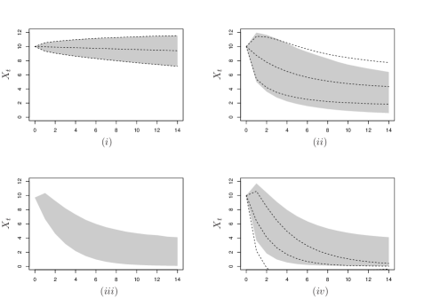
Figure 1: Four Markov chains in exponential margins with different dependence structure and common initial extreme value of $x_{0}=10$. Presented for each chain are: 2.5% and 97.5% quantiles of the actual chain $\{X_{t}\}$ started from $x_{0}=10$ (grey region); 2.5% quantile, mean and 97.5% quantile of the approximating chain $\{X^{TC}_{t}\}$ arising from the tail chain with $x_{0}=10$ (dashed lines, apart from (iii)). The copula of $(X_{t},X_{t+1})$ comes from: (i): BEV copula, with logistic dependence structure, $\gamma=0.152$, (ii): inverted BEV copula with logistic dependence structure, $\gamma=0.152$, (iii): exponential auto-regressive process with $\phi=0.8$, (iv): Gaussian copula with $\rho=0.8$.

The parameters for chains (ii) and (iv) have been chosen such that the coefficient of tail dependence Ledford and Tawn (1997) of the bivariate margins is the same. The plots compare the actual Markov chain $\{X_{t}\}$ started from $X_{0}=10$ with the paths $\{X^{TC}_{t}\}$ arising from the tail chain approximation $X_{t}^{TC}=a_{t}(X_{0})+b_{t}(X_{0})M_{t}$, where $a_{t}$, $b_{t}$ and $M_{t}$ are as defined in Example 2 and determined by the associated value of $(\alpha,\beta)$ and the respective limiting kernel $K$. The figure shows both the effect of the different normalizations on the sample paths and that the limiting tail chains provide a reasonable approximation to the tail chain for this level of $X_{0}$, at least for the first few steps. Unfortunately, we were not able to derive the limiting kernel $K$ from (iii) and so the limiting tail chain approximation $\{X^{TC}_{t}\}$ is not shown in this case. Also note that for the asymptotically independent processes and chain (iv) in particular, there is some discrepancy between the actual and the approximating limiting chains. This difference is due to the slow convergence to the limit here, a feature identified in the multivariate context by Heffernan and Tawn (2004) for chain (iv), but this property can occur similarly for asymptotically dependent processes.

4 Extensions

In this section, we address several phenomena which have not yet been covered by the preceding theory. The information stored in the value $X_{0}$ is often not good enough for assertions on the future due to additional sources of randomness that influence the return to the body of the marginal distribution or switching to a negative extreme state. Let us assume, for instance, that the transition kernel of a Markov chain encapsulates different modes of normalization. If we use our previous normalization scheme matching the dominating mode, the tail chain will usually terminate in a degenerate state. In order to gain non-degenerate limits which allow for a refined analysis in such situations, we will introduce random change-points that can detect the misspecification of the norming and adapt the normings accordingly after change-points. The first of the change-points plays a similar role to the extremal boundary in Resnick and Zeber (2013). We also use this concept to resolve some of the subtleties arising from random negative dependence. The resulting limiting processes $\{M_{t}\,:\,t=1,2,\dots\}$ of

$$\left\{\frac{X_{t}-a_{t}(X_{0})}{b_{t}(X_{0})}\,:\,t=1,2,\dots\right\}\,\bigg{|}\,X_{0}>u$$

as $u\uparrow\infty$ (with limits meant in finite-dimensional distributions) will be termed hidden tail chains if they are based on change-points and adapted normings, even though $\{M_{t}\}$ need not be first order Markov chains anymore due to additional sources of randomness in their update schemes. However, they reveal additional (“hidden”) structure after certain change-points. We present such phenomena in the sequel by means of some examples which successively reveal increasing complex structure. Weak convergence will be meant on the extended real line including $\pm\infty$ if mass escapes to these states.

4.1 Hidden tail chains

Mixtures of different modes of normalization

Example 5.

(Bivariate extreme value copula with asymmetric logistic dependence)
The transition kernel $\pi_{F}$ arising from a bivariate extreme value distribution with asymmetric logistic distribution on Fréchet scale (Tawn, 1988) is given by

$$\pi_{F}(x,y)=-x^{2}\frac{\partial}{\partial x}V(x,y)\exp\bigg{(}\frac{1}{x}-V(x,y)\bigg{)},$$

where $V(x,y)$ is the exponent function

$$V(x,y)=\frac{1-\varphi_{1}}{x}+\frac{1-\varphi_{2}}{y}+\bigg{\{}\Big{(}\frac{\varphi_{1}}{x}\Big{)}^{1/\nu}+\Big{(}\frac{\varphi_{2}}{y}\Big{)}^{1/\nu}\bigg{\}}^{\nu},\qquad\varphi_{1},\varphi_{2},\nu\in(0,1).$$

Changing the marginal scale from standard Fréchet to standard exponential margins yields the transition kernel

$$\pi(x,y)=\pi_{F}(T(x),T(y)),\quad\text{where}\quad T(x)=-1/\log\left(1-\exp(-x)\right).$$

The kernel $\pi$ converges weakly with two distinct normalizations

$$\pi(v,v+dx)\stackrel{{\scriptstyle\mathcal{D}}}{{\rightarrow}}K_{1}(dx)\quad\text{and}\quad\pi(v,dx)\stackrel{{\scriptstyle\mathcal{D}}}{{\rightarrow}}K_{2}(dx)\qquad\text{as $v\uparrow\infty$}$$

to the distributions

$$K_{1} =(1-\varphi_{1})\delta_{-\infty}+\varphi_{1}G_{1},\qquad\,G_{1}(x)=\bigg{[}1+\bigg{\{}\frac{\varphi_{2}}{\varphi_{1}}\exp(-x)\bigg{\}}^{1/\nu}\bigg{]}^{\nu-1}$$

$$K_{2} =(1-\varphi_{1})F_{E}+\varphi_{1}\delta_{+\infty},\qquad F_{E}(x)=\left(1-\exp(-x)\right)_{+}$$

with entire mass on $[-\infty,\infty)$ and $(0,\infty]$, respectively. In the first normalization, mass of the size $1-\varphi_{1}$ escapes to $-\infty$, whereas in the second normalization the complementary mass $\varphi_{1}$ escapes to $+\infty$ instead. The reason for this phenomenon is that both normalizations are related to two different modes of the conditioned distribution of $X_{t+1}\mid X_{t}$ of the Markov chain, cf. Figure 2. However, these two modes can be separated, for instance, by any line of the form $(x_{t},cx_{t})$ for some $c\in(0,1)$ as illustrated in Figure 2 with $c=1/2$. This makes it possible to account for the mis-specification in the two normings above by introducing the change-point

$$T^{X}=\inf\left\{t\geq 1\,:\,X_{t}\leq cX_{t-1}\right\},$$ (4)

i.e., $T^{X}$ is the first time that $c$ times the previous state is not exceeded anymore. Adjusting the above normings to

$$a_{t}(v) =\begin{cases}v&\quad t<T^{X},\\ 0&\quad t\geq T^{X},\end{cases}\quad\text{and}\quad b_{t}(v)=1,$$

yields the following hidden tail chain, which is built on an independent i.i.d. sequence $\{B_{t}\,:\,t=1,2,\dots\}$ of latent Bernoulli random variables $B_{t}\sim\text{Ber}(\varphi_{1})$ and the hitting time $T^{B}=\inf\{t\geq 1\,:\,B_{t}=0\}$. Its initial distribution is given by

$$\Pr(M_{1}\leq x)=\begin{cases}G_{1}(x)&\quad T^{B}>1,\\ F_{E}(x)&\quad T^{B}=1,\end{cases}$$

and its transition mechanism is

$$\Pr(M_{t}\leq y\mid M_{t-1}=x)=\begin{cases}G_{1}(y-x)&\quad t<T^{B},\\ F_{E}(y)&\quad t=T^{B},\\ \pi(x,y)&\quad t>T^{B}.\end{cases}$$

In other words, the tail chain behaves like a random walk with innovations from $K_{1}$ as long as it does not hit the value $-\infty$ and, if it does, the norming changes instead, such that the original transition mechanism of the Markov chain is started again from an independent exponential random variable.

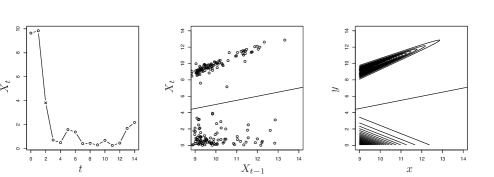
Figure 2: Left: time series plot showing a single realisation from the Markov chain with asymmetric logistic dependence, initialised from the distribution $X_{0}\mid X_{0}>9$. The change-point $T^{X}=2$ with $c=1/2$ (cf. Eq. (4)) is highlighted with a cross. Centre: scatterplot of consecutive states $(X_{t-1},X_{t})$, for $t=1,\ldots,T^{X}$ with $c=1/2$, drawn from 1000 realisations of the Markov chain initialised from $X_{0}\mid X_{0}>9$ and line $X_{t}=X_{t-1}/2$ superposed. Right: Contours of joint density of asymmetric logistic distribution with exponential margins and line $y=x/2$ superposed. The asymmetric logistic parameters used are $\varphi_{1}=\varphi_{2}=0.5$ and $\gamma=0.152$.

In Example 5 the adjusted tail chain starts as a random walk and then permanently terminates in the transition mechanism of the original Markov chain after a certain change-point that can distinguish between two different modes of normalization. These different modes arise as the conditional distribution of $X_{t+1}|X_{t}$ is essentially a mixture distribution when $X_{t}$ is large with one component of the mixture returning the process to a non-extreme state.

The following example extends this mixture structure to the case where both components of the mixture keep the process in an extreme state, but with different Heffernan and Tawn canonical family norming needed for each component. The first component gives the strongest form of extremal dependence. The additional complication that this creates is that there is now a sequence of change-points, as the process switches from one component to the other, and the behaviour of the resulting tail chain subtly changes between these.

Example 6.

(Mixtures from the canonical Heffernan-Tawn model)
For two transition kernels $\pi_{1}$ and $\pi_{2}$ on the standard exponential scale, each stabilizing under the Heffernan-Tawn normalization

$$\pi_{1}(v,\alpha_{1}v+v^{\beta_{1}}dx)\stackrel{{\scriptstyle\mathcal{D}}}{{\rightarrow}}G_{1}(dx)\quad\text{and}\quad\pi_{2}(v,\alpha_{2}v+v^{\beta_{2}}dx)\stackrel{{\scriptstyle\mathcal{D}}}{{\rightarrow}}G_{2}(dx)$$

as in Example 2 (ii) for $v\uparrow\infty$, let us consider the mixed transition kernel

$$\pi=\lambda\,\pi_{1}+(1-\lambda)\,\pi_{2},\qquad\lambda\in(0,1).$$

Assuming that $\alpha_{1}>\alpha_{2}$, the kernel $\pi$ converges weakly on the extended real line with the two distinct normalizations

$$\pi(v,\alpha_{1}v+v^{\beta_{1}}dx)\stackrel{{\scriptstyle\mathcal{D}}}{{\rightarrow}}K_{1}(dx)\quad\text{and}\quad\pi(v,\alpha_{2}v+v^{\beta_{2}}dx)\stackrel{{\scriptstyle\mathcal{D}}}{{\rightarrow}}K_{2}(dx)\qquad\text{as $v\uparrow\infty$}$$

to the distributions $K_{1}=\lambda G_{1}+(1-\lambda)\delta_{-\infty}$ and $K_{2}=(1-\lambda)G_{2}+\lambda\delta_{+\infty}$, with mass $(1-\lambda)$ escaping to $-\infty$ in the first case and complementary mass $\lambda$ to $+\infty$ in the second case. Similarly to Example 5, the different modes of normalization for the consecutive states $(X_{t},X_{t+1})$ are increasingly well separated by any line of the form $(x_{t},{cx_{t}})$ with $c\in(\alpha_{2},\alpha_{1})$. In this situation, the following recursively defined sequence of change-points

$$T_{1}^{X} =\inf\left\{t\geq 1\,:\,X_{t}\leq cX_{t-1}\right\}$$

$$T_{k+1}^{X} =\begin{cases}\inf\left\{t\geq T^{X}_{k}+1\,:\,X_{t}>cX_{t-1}\right\}&\quad k\text{ odd},\\ \inf\left\{t\geq T^{X}_{k}+1\,:\,X_{t}\leq cX_{t-1}\right\}&\quad k\text{ even}\end{cases}$$

and the normings

$$a_{t}(v)=n^{\alpha}_{t}v,\quad b_{t}(v)=\begin{cases}v^{\beta_{1}}&\quad t<T^{X}_{1},\\ v^{\beta_{2}}&\quad T^{X}_{1}=1\text{ and }t<T^{X}_{2},\\ v^{\max\{\beta_{1},\beta_{2}\}}&\quad t\geq T^{X}_{1},\text{ unless }T^{X}_{1}=1\text{ and }t<T^{X}_{2}\end{cases}$$

with

$$n^{\alpha}_{t}=\begin{cases}\alpha^{t}_{1}&t<T^{X}_{1},\\ \alpha_{1}^{(S_{k}^{\text{odd}}-1)-S_{k}^{\text{even}}}\alpha_{2}^{t+S_{k}^{\text{even}}-(S_{k}^{\text{odd}}-1)}&T^{X}_{k}\leq t<T^{X}_{k+1},\,k\text{ odd},\\ \alpha_{1}^{t+S_{k}^{\text{odd}}-S_{k}^{\text{even}}}\alpha_{2}^{S_{k}^{\text{even}}-S_{k}^{\text{odd}}}&T^{X}_{k}\leq t<T^{X}_{k+1},\,k\text{ even},\end{cases}$$

and

$$S_{k}^{\text{odd/even}}=\sum_{\begin{subarray}{c}j=1,\dots,k,\\ j\text{ odd/even}\end{subarray}}T_{j}^{X}$$

leads to a variety of transitions into less extreme states, depending on the ordering of $\beta_{2}$ and $\beta_{1}$. As in Example 5, the hidden tail chain can be based again on a set of latent Bernoulli variables $\{B_{t}\,:\,t=1,2,\dots\}$ with $B_{t}\sim\text{Ber}(\lambda)$. It has the initial distribution

$$M_{1}\sim\begin{cases}G_{1}&\quad T^{B}_{1}>1,\\ G_{2}&\quad T^{B}_{1}=1,\end{cases}$$

and is not a first order Markov chain anymore, as its transition scheme takes the position among the change-points

$$T^{B}_{1} =\inf\{t\geq 1\,:\,B_{t}\neq B_{t-1}\}$$

$$T^{B}_{k+1} =\inf\{t\geq T^{B}_{k}+1\,:\,B_{t}\neq B_{t-1}\},\quad k=1,2,\dots,$$

into account as follows

$$M_{t+1}=\begin{cases}\alpha_{1}M_{t}+(n^{\alpha}_{t})^{\beta_{1}}\varepsilon_{t}^{(1)}&\quad t+1<T^{B}_{1}\text{ or }T^{B}_{k}\leq t+1<T^{B}_{k+1},\,k\text{ even},\,\beta_{1}\geq\beta_{2},\\[-2.84526pt] &\quad\text{unless }T^{B}_{1}=1,\,t+1=T^{B}_{2}\text{ and }\beta_{1}>\beta_{2},\\[-2.84526pt] \alpha_{2}M_{t}+(n^{\alpha}_{t})^{\beta_{2}}\varepsilon_{t}^{(2)}&\quad T^{B}_{1}=1\text{ and }t+1<T^{B}_{2},\,\beta_{1}>\beta_{2},\\[-2.84526pt] &\quad\text{or }T^{B}_{k}\leq t+1<T^{B}_{k+1},\,k\text{ odd},\,\beta_{1}\leq\beta_{2},\\[-2.84526pt] &\quad\text{unless }t+1=T_{1}\text{ and }\beta_{1}<\beta_{2},\\[-2.84526pt] (n^{\alpha}_{t})^{\beta_{1}}\varepsilon_{t}^{(1)}&\quad T^{B}_{1}=1\text{ and }t+1=T^{B}_{2},\,\beta_{1}>\beta_{2},\\[-2.84526pt] (n^{\alpha}_{t})^{\beta_{2}}\varepsilon_{t}^{(2)}&\quad t+1=T^{B}_{1},\,\beta_{1}<\beta_{2},\\[-2.84526pt] \alpha_{1}M_{t}&\quad T^{B}_{k}\leq t+1<T^{B}_{k+1},\,k\text{ even},\,\beta_{1}<\beta_{2},\\[-2.84526pt] \alpha_{2}M_{t}&\quad T^{B}_{k}\leq t+1<T^{B}_{k+1},\,k\text{ odd},\,\beta_{1}>\beta_{2},\\[-2.84526pt] &\quad\text{unless }T^{B}_{1}=1,\,k=1\text{ and }\beta_{1}>\beta_{2}.\end{cases}$$

The independent innovations are drawn from either $\varepsilon_{t}^{(1)}\sim G_{1}$ or $\varepsilon_{t}^{(2)}\sim G_{2}$. The hidden tail chain can transition into a variety of forms depending on the characteristics of the transition kernels $\pi_{1}$ and $\pi_{2}$. According to the ordering of the scaling power parameters $\beta_{1},\beta_{2}$, the tail chain at the transition points can degenerate to a scaled value of the previous state or independent of previous values.

Returning chains

Finally, we consider Markov processes which can return to extreme states. Examples include tail switching processes, i.e., processes that are allowed to jump between the upper and lower tail of the marginal stationary distribution of the process. To facilitate comparison, we use the standard Laplace distribution

$$F_{L}(x)=\left\{\begin{array}[]{ll}\frac{1}{2}\exp(x)&\quad x<0,\\ 1-\frac{1}{2}\exp(-x)&\quad x\geq 0.\end{array}\right.$$ (7)

as a common marginal, so that both lower and upper tail is of the same exponential type.

Example 7.

(Rootzén/Smith tail switching process with Laplace margins)
As in Smith (1992) and adapted to our chosen marginal scale, consider the stationary Markov process that is initialised from the standard Laplace distribution and with transition mechanism built on independent i.i.d. sequences of standard Laplace variables $\{L_{t}\,:\,t=0,1,2,\dots\}$ and Bernoulli variables $\{B_{t}\,:\,t=0,1,2,\dots\}$ with $B_{t}\sim\text{Ber}(0.5)$ as follows

$$X_{t+1}=-B_{t}X_{t}+(1-B_{t})L_{t}=\begin{cases}-X_{t}&\quad B_{t}=1,\\ L_{t}&\quad B_{t}=0.\end{cases}$$

The following convergence situations arise as $X_{0}$ goes to its upper or lower tail

$$X_{1}+X_{0}\mid X_{0}=x_{0} \stackrel{{\scriptstyle\mathcal{D}}}{{\rightarrow}}\begin{cases}0.5\,(\delta_{0}+\delta_{+\infty})&\,\,\quad x_{0}\uparrow+\infty,\\ 0.5\,(\delta_{-\infty}+\delta_{0})&\,\,\quad x_{0}\downarrow-\infty,\end{cases}$$

$$X_{1}\mid X_{0}=x_{0} \stackrel{{\scriptstyle\mathcal{D}}}{{\rightarrow}}\begin{cases}0.5\,(\delta_{-\infty}+F_{L})&\quad x_{0}\uparrow+\infty,\\ 0.5\,(F_{L}+\delta_{\infty})&\quad x_{0}\downarrow-\infty,\end{cases}$$

where, in addition to their finite components $\delta_{0}$ and $F_{L}$, the limiting distributions collect complementary masses at $\pm\infty$. Introducing the change-point

$$T^{X}=\inf\{t\geq 1\,:\,X_{t}\neq X_{t-1}\}$$

and adapted time-dependent normings

$$a_{t}(v)=\begin{cases}(-1)^{t}v&\quad t<T^{X},\\ 0&\quad t\geq T^{X},\end{cases}\quad\text{and}\quad b_{t}(v)=1,$$

leads to the tail chain

$$M_{t}=\begin{cases}0&\quad t<T^{X},\\ X^{\prime}_{t-T^{X}}&\quad t\geq T^{X},\end{cases}$$

where $\{X^{\prime}_{t}\,:\,t=0,1,2,\dots\}$ is a copy of the original Markov chain $\{X_{t}\,:\,t=0,1,2,\dots\}$.

Example 7 illustrates that the Markov chain can return to the extreme states visited before the termination time, it strictly alternates between $X_{0}$ and $-X_{0}$. Similarly with Example 5, the hidden tail chain permanently terminates in finite time and the process jumps to a non-extreme event in the stationary distribution of the process. The next example shows a tail switching process with non-degenerate tail chain that does not suddenly terminate.

Example 8.

(ARCH with Laplace margins)
In its original scale the ARCH(1) process $\{Y_{t}\,:\,t=0,1,2,\dots\}$ follows the transition scheme $Y_{t}=\left(\theta_{0}+\theta_{1}\,Y_{t-1}^{2}\right)^{1/2}W_{t}$ for some $\theta_{0}>0$, $0<\theta_{1}<1$ and an i.i.d. sequence $\{W_{t}\,:\,t=0,1,2,\dots\}$ of standard Gaussian variables. It can be shown that, irrespectively of how the process is initialised, it converges to a stationary distribution $F_{\infty}$, whose lower and upper tail are asymptotically equivalent to a Pareto tail, i.e.,

$$1-F_{\infty}(x)=F_{\infty}(-x)\doteq cx^{-\kappa}\qquad\text{as }x\uparrow\infty,$$

for some $c,\kappa>0$ (de Haan et al., 1989). Initialising the process from $F_{{\infty}}$ yields a stationary Markov chain, whose transition kernel becomes

$$\pi(x,y)=\Phi\left(\frac{F^{\leftarrow}_{\infty}(F_{L}(y))}{(\theta_{0}+\theta_{1}(F_{\infty}^{\leftarrow}(F_{L}(x)))^{2})^{1/2}}\right)$$

if the chain is subsequently transformed to standard Laplace margins. It converges with two distinct normalizations

$$\pi(v,v+dx)\stackrel{{\scriptstyle\mathcal{D}}}{{\rightarrow}}\begin{cases}K_{+}(dx)&\quad v\uparrow+\infty,\\ K_{-}(dx)&\quad v\downarrow-\infty,\end{cases}$$

$$\pi(v,-v+dx)\stackrel{{\scriptstyle\mathcal{D}}}{{\rightarrow}}\begin{cases}K_{-}(dx)&\quad v\uparrow+\infty,\\ K_{+}(dx)&\quad v\downarrow-\infty\end{cases}$$

to the distributions $K_{+}=0.5(\delta_{-\infty}+G_{+})$ and $K_{-}=0.5(G_{-}+\delta_{+\infty})$ with

$$G_{+}(x)=2\Phi\left(\frac{\exp(x/\kappa)}{\sqrt{\theta_{1}}}\right)-1\quad\text{and}\quad G_{-}(x)=2\Phi\left(-\frac{\exp(-x/\kappa)}{\sqrt{\theta_{1}}}\right).$$

Here, the recursively defined sequence of change-points

$$T^{X}_{1} =\inf\{t\geq 1\,:\,\text{sign}(X_{t})\neq\text{sign}(X_{t-1})\}$$

$$T^{X}_{k+1} =\inf\{t\geq T^{X}_{k}+1\,:\,\text{sign}(X_{t})\neq\text{sign}(X_{t-1})\},\quad k=1,2,\dots,$$

which documents the sign change, and adapted normings

$$a_{t}(v)=\begin{cases}v&\quad t<T^{X}_{1}\text{ or }T^{X}_{k}\leq t<T^{X}_{k+1},\,k\text{ even},\\ -v&\quad\phantom{t<T^{X}_{1}\text{ or }}T^{X}_{k}\leq t<T^{X}_{k+1},\,k\text{ odd,}\end{cases}\qquad b_{t}(v)=1,$$

lead to a hidden tail chain (which is not a first order Markov chain anymore) as follows. It is distributed like a sequence $\{M_{t}\,:\,t=1,2,\dots\}$ built on the change-points

$$T^{B}_{1} =\inf\{t\geq 1\,:\,B_{t}\neq B_{t-1}\}$$

$$T^{B}_{k+1} =\inf\{t\geq T^{B}_{k}+1\,:\,B_{t}\neq B_{t-1}\},\quad k=1,2,\dots,$$

of an i.i.d. sequence of Bernoulli variables $\{B_{t}\,:\,t=1,2,\dots\}$ via the initial distribution

$$M_{1}\sim\begin{cases}G_{+}&\quad T^{B}_{1}>1,\\ G_{-}&\quad T^{B}_{1}=1,\end{cases}$$

and transition scheme

$$M_{t+1}=s_{t}M_{t}+\varepsilon_{t},$$

where the sign $s_{t}$ is negative at change-points

$$s_{t}=\begin{cases}-1&\quad t+1=T^{B}_{k}\text{ for some }k=1,2,\dots,\\ 1&\quad\text{else},\end{cases}$$

and the independent innovations $\varepsilon_{t}$ are drawn from either $G_{+}$ or $G_{-}$ according to the position of $t+1$ within the intervals between change-points

$$\varepsilon_{t}\sim\begin{cases}G_{+}&\quad t+1<T^{B}_{1}\text{ or }T^{B}_{k}\leq t+1<T^{B}_{k+1},\,k\text{ even},\\ G_{-}&\quad\phantom{t+1<T^{B}_{1}\text{ or }}T^{B}_{k}\leq t+1<T^{B}_{k+1},\,k\text{ odd}.\end{cases}$$

Remark 6.

An alternative tail chain approach to Example 8 is to square the ARCH process, $Y_{t}^{2}$ instead of $Y_{t}$, which leads to a random walk tail chain as discussed in Resnick and Zeber (2013). An advantage of our approach is that we may condition on an upper (or by symmetry lower) extreme state whereas in the squared process this information is lost and one has to condition on its norm being large.

4.2 Negative dependence

In the previous examples the change from upper to lower extremes and vice versa has been driven by a latent Bernoulli random variable. If the consecutive states of a time series are negatively dependent, such switchings are almost certain. An example is the autoregressive Gaussian Markov chain in Example 1, in which case the tail chain representation there trivially remains true even if the correlation parameter $\rho$ varies in the negatively dependent regime $(-1,0)$. More generally, our previous results may be transferred to Markov chains with negatively dependent consecutive states when interest lies in both upper extreme states and lower extreme states. For instance, the conditions for Theorem 1 may be adapted as follows.

Assumption C1

(behaviour of the next state as the previous state becomes extreme)
There exist measurable norming functions $a_{-}(v),a_{+}(v)\in\mathbb{R}$, $b_{-}(v),b_{+}(v)>0$ and non-degenerate distribution functions $K_{-}$, $K_{+}$ on $\mathbb{R}$, such that

$$\pi(v,a_{-}(v)+b_{-}(v)dx)\stackrel{{\scriptstyle\mathcal{D}}}{{\rightarrow}}K_{-}(dx)\qquad\text{as }v\uparrow\infty,$$

$$\pi(v,a_{+}(v)+b_{+}(v)dx)\stackrel{{\scriptstyle\mathcal{D}}}{{\rightarrow}}K_{+}(dx)\qquad\text{as }v\downarrow-\infty.$$

Assumption C2

(norming functions and update functions for the tail chain)

1. Additionally to $a_{1}=a_{-}$ and $b_{1}=b_{-}$ assume there exist measurable norming functions $a_{t}(v)\in\mathbb{R}$, $b_{t}(v)>0$ for $t=2,3,\dots$, such that, for all $x\in\mathbb{R}$, $t=1,2,\dots$

   $$a_{t}(v)+b_{t}(v)x\rightarrow\left\{\begin{array}[]{ll}-\infty&\quad\text{$t$ odd,}\\ \infty&\quad\text{$t$ even,}\end{array}\right.\qquad\text{as }v\uparrow\infty.$$

2. Set

   $$\widehat{a}_{t}=\begin{cases}a_{+}&\quad t\text{ odd},\\ a_{-}&\quad t\text{ even},\end{cases}\quad\text{and}\quad\widehat{b}_{t}=\begin{cases}b_{+}&\quad t\text{ odd},\\ b_{-}&\quad t\text{ even}.\end{cases}$$

   and assume further that there exist continuous update functions

   $$\psi_{t}^{a}(x) =\lim_{v\rightarrow\infty}\frac{\widehat{a}_{t}\left(a_{t}(v)+b_{t}(v)x\right)-a_{t+1}(v)}{b_{t+1}(v)}\in\mathbb{R},$$

   $$\psi_{t}^{b}(x) =\lim_{v\rightarrow\infty}\frac{\widehat{b}_{t}\left(a_{t}(v)+b_{t}(v)x\right)}{b_{t+1}(v)}>0,$$

   defined for $x\in\mathbb{R}$ and $t=1,2,\dots$, such that the remainder terms

   $$r^{a}_{t}(v,x) =\frac{a_{t+1}(v)-\widehat{a}_{t}(a_{t}(v)+b_{t}(v)x)+b_{t+1}(v)\psi^{a}_{t}(x)}{\widehat{b}_{t}(a_{t}(v)+b_{t}(v)x)},$$

   $$r^{b}_{t}(v,x) =1-\frac{b_{t+1}(v)\psi^{b}_{t}(x)}{\widehat{b}_{t}(a_{t}(v)+b_{t}(v)x)}$$

   converge to $0$ as $v\to\infty$ and both convergences hold uniformly on compact sets in the variable $x\in\mathbb{R}$.

Using the proof of Theorem 1, it is straightforward to check that the following version adapted to negative dependence holds true.

Theorem 3.

Let $\{X_{t}\,:\,t=0,1,2,\dots\}$ be a homogeneous Markov chain satisfying assumption F₀ , C1 and C2. Then, as $u\uparrow\infty$,

$$\left(\frac{X_{0}-u}{\sigma(u)},\frac{X_{1}-a_{1}(X_{0})}{b_{1}(X_{0})},\frac{X_{2}-a_{2}(X_{0})}{b_{2}(X_{0})},\dots,\frac{X_{t}-a_{t}(X_{0})}{b_{t}(X_{0})}\right)\,\bigg{|}\,X_{0}>u$$

converges weakly to $\left(E_{0},M_{1},M_{2},\dots,M_{t}\right)$, where

1. $E_{0}\sim H_{0}$ and $(M_{1},M_{2},\dots,M_{t})$ are independent,

2. $M_{1}\sim K_{-}$ and $M_{t+1}=\psi^{a}_{t}(M_{j})+\psi^{b}_{t}(M_{t})\,\varepsilon_{t},\,t=1,2,\dots$ for an independent sequence of innovations

   $$\varepsilon_{t}\sim\left\{\begin{array}[]{ll}K_{+}&\quad\text{$t$ odd,}\\ K_{-}&\quad\text{$t$ even.}\end{array}\right.$$

Remark 7.

Due to different limiting behaviour of upper and lower tails, the tail chain $\{M_{t}\,:\,t=0,1,2,\dots\}$ from Theorem 3 has a second source of potential non-homogeneity, since the innovations $\varepsilon_{t}$ will be generally not i.i.d. anymore, cf. also Remark 5.

Example 9.

(Heffernan-Tawn normalization in case of negative dependence)
Consider a stationary Markov chain with standard Laplace margins (7) and transition kernel $\pi$ satisfying

$$\pi(v,\alpha_{-}v+|v|^{\beta}dx)\stackrel{{\scriptstyle\mathcal{D}}}{{\rightarrow}}K_{-}(dx)\qquad\text{as }v\uparrow\infty,$$

$$\pi(v,\alpha_{+}v+|v|^{\beta}dx)\stackrel{{\scriptstyle\mathcal{D}}}{{\rightarrow}}K_{+}(dx)\qquad\text{as }v\downarrow-\infty.$$

for some $\alpha_{-},\alpha_{+}\in(-1,0)$ and $\beta\in[0,1)$. Then the normalization after $t$ steps

$$a_{t}(v) =\left\{\begin{array}[]{ll}\alpha_{-}^{(t+1)/2}\alpha_{+}^{(t-1)/2}v&\quad\text{$t$ odd,}\vskip 6.0pt plus 2.0pt minus 2.0pt\\ \alpha_{-}^{t/2}\alpha_{+}^{t/2}v&\quad\text{$t$ even,}\end{array}\right.$$

$$b_{t}(v) =|v|^{\beta}$$

yields the tail chain

$$M_{t+1}=\left\{\begin{array}[]{ll}\alpha_{+}M_{t}+\left\lvert\alpha_{-}^{(t+1)/2}\alpha_{+}^{(t-1)/2}\right\rvert^{\beta}\varepsilon_{t}^{+}&\quad\text{$t$ odd,}\vskip 6.0pt plus 2.0pt minus 2.0pt\\ \alpha_{-}M_{t}+\left\lvert\alpha_{-}^{t/2}\alpha_{+}^{t/2}\right\rvert^{\beta}\varepsilon_{t}^{-}&\quad\text{$t$ even,}\end{array}\right.$$

with independent innovations $\varepsilon_{t}^{+}\sim K_{+}$ and $\varepsilon_{t}^{-}\sim K_{-}$.

Example 10.

(negatively dependent Gaussian transition kernel with Laplace margins)
Consider as in Example 1 a stationary Gaussian Markov chain with standard Laplace margins and $\rho\in(-1,0)$. Assumption C1 is satisfied with $a_{-}(v)=a_{+}(v)=-\rho^{2}v$, $b_{-}(v)=b_{+}(v)=v^{1/2}$ and $K(x)=K_{-}(x)=K_{+}(x)=\Phi\left(x/(2\rho^{2}(1-\rho^{2}))^{1/2}\right)$. Then the normalization after $t$ steps $a_{t}(v)=(-1)^{t}\rho^{2t}v$ and $b_{t}(v)=|v|^{\beta}$ yields the tail chain $M_{t+1}=-\rho^{2}M_{t}+(-\rho)^{t}\varepsilon_{t}$ with independent innovations $\varepsilon_{t}\sim K$.

Remark 8.

If the $\beta$-parameter of the Heffernan-Tawn normalization in Example 9 is different for lower and upper extreme values, one encounters similar varieties of different behaviour as in Example 6.

5 Proofs

5.1 Proofs for Section 2

Some techniques in the followings proofs are analogous to Kulik and Soulier (2015) with adaptions to our situation including the random norming as in Janßen and Segers (2014). By contrast to previous accounts, we have to control additional remainder terms, which make the auxiliary Lemma 8 necessary. The following result is a preparatory lemma and the essential part of the induction step in the proof of Theorem 1.

Lemma 4.

Let $\{X_{t}\,:\,t=0,1,2,\dots\}$ be a homogeneous Markov chain satisfying assumptions A1 and A2. Let $g\in C_{b}(\mathbb{R})$. Then, for $t=1,2,\dots$, as $v\uparrow\infty$,

$$\int_{\mathbb{R}}g(y)\pi(a_{t}(v)+b_{t}(v)x,a_{t+1}(v)+b_{t+1}(v)dy)\rightarrow\int_{\mathbb{R}}g(\psi^{a}_{t}(x)+\psi^{b}_{t}(x)y)K(dy)$$ (8)

and the convergence holds uniformly on compact sets in the variable $x\in\mathbb{R}$.

Proof.

Let us fix $t\in\mathbb{N}$. We start by noticing

$$a_{t+1}(v)+b_{t+1}(v)y$$

$$=a(a_{t}(v)+b_{t}(v)x)+b(b_{t}(v)x+a_{t}(v))\,\left[r^{a}_{t}(v,x)+\left(1-r^{b}_{t}(v,x)\right)\,\frac{y-\psi^{a}_{t}(x)}{\psi^{b}_{t}(x)}\right].$$

Hence the left-hand side of (8) can be rewritten as

$$\int_{\mathbb{R}}g(y)\pi(a_{t}(v)+b_{t}(v)x,a_{t+1}(v)+b_{t+1}(v)dy)$$

$$=\int_{\mathbb{R}}g\left(\psi^{a}_{t}(x)+\psi^{b}_{t}(x)\frac{y-r^{a}_{t}(v,x)}{1-r^{b}_{t}(v,x)}\right)\pi(A_{t}(v,x),a(A_{t}(v,x))+b(A_{t}(v,x))\,dy))$$

$$=\int_{\mathbb{R}}f_{v}(x,y)\,\pi_{v,x}(dy)$$

if we abbreviate

$$A_{t}(v,x) =a_{t}(v)+b_{t}(v)x,$$

$$\pi_{x}(dy) =\pi(x,a(x)+b(x)\,dy),$$

$$\pi_{v,x}(dy) =\pi_{A_{t}(v,x)}(dy),$$

$$f(x,y) =g\left(\psi^{a}_{t}(x)+\psi^{b}_{t}(x)y\right),$$

$$f_{v}(x,y) =f\left(x,\frac{y-r^{a}_{t}(v,x)}{1-r^{b}_{t}(v,x)}\right),$$

and we need to show that for compact $C\subset\mathbb{R}$

$$\sup_{x\in C}\left\lvert\int_{\mathbb{R}}f_{v}(x,y)\pi_{v,x}(dy)-\int_{\mathbb{R}}f(x,y)K(dy)\right\rvert\rightarrow 0\qquad\text{as }v\uparrow\infty.$$

In particular it suffices to show the slightly more general statement that

$$\sup_{c_{1}\in C_{1}}\sup_{c_{2}\in C_{2}}\left\lvert\int_{\mathbb{R}}f_{v}(c_{1},y)\pi_{v,c_{2}}(dy)-\int_{\mathbb{R}}f(c_{1},y)K(dy)\right\rvert\rightarrow 0\qquad\text{as }v\uparrow\infty,$$

for compact sets $C_{1},C_{2}\subset\mathbb{R}$. Using the inequality

$$\left\lvert\int_{\mathbb{R}}f_{v}(c_{1},y)\pi_{v,c_{2}}(dy)-\int_{\mathbb{R}}f(c_{1},y)K(dy)\right\rvert$$

$$\leq\int_{\mathbb{R}}\left\lvert f_{v}(c_{1},y)-f(c_{1},y)\right\rvert\pi_{v,c_{2}}(dy)+\left\lvert\int_{\mathbb{R}}f(c_{1},y)\pi_{v,c_{2}}(dy)-\int_{\mathbb{R}}f(c_{1},y)K(dy)\right\rvert,$$

the preceding statement will follow from the following two steps.
1st step We show

$$\sup_{c_{2}\in C_{2}}\int_{\mathbb{R}}\left(\sup_{c_{1}\in C_{1}}\left\lvert f_{v}(c_{1},y)-f(c_{1},y)\right\rvert\right)\,\pi_{v,c_{2}}(dy)\rightarrow 0\qquad\text{as }v\uparrow\infty.$$

Let $\varepsilon>0$ and let $M$ be an upper bound for $g$, such that $2M$ is an upper bound for $\lvert f_{v}-f\rvert$. Due to assumption A1 and Lemma 7 there exists $L=L_{\varepsilon,M}\in\mathbb{R}$ and a compact set $C=C_{\varepsilon,M}\subset\mathbb{R}$, such that $\pi_{\ell}(C)>1-\varepsilon/(2M)$ for all $\ell\geq L$. Because of assumption A2 (a) there exists $V=V_{L}\in\mathbb{R}$ such that $A_{t}(v,c_{2})\geq A_{t}(v,\min(C_{2}))\geq L$ for all $v\geq V$, $c_{2}\in C_{2}$. Hence

$$\pi_{v,c_{2}}(C)>1-\varepsilon/(2M)\quad\text{ for all }v\geq V,\,c_{2}\in C_{2}.$$

Moreover, by assumption A2 (b) the map

$$\mathbb{R}\times\mathbb{R}\ni(x,y)\mapsto\psi^{a}_{t}(x)+\psi^{b}_{t}(x)\frac{y-r^{a}_{t}(v,x)}{1-r^{b}_{t}(v,x)}\in\mathbb{R}$$

converges uniformly on compact sets to the map

$$\mathbb{R}\times\mathbb{R}\ni(x,y)\mapsto\psi^{a}_{t}(x)+\psi^{b}_{t}(x)y\in\mathbb{R}.$$

Since the latter map is continuous by assumption A2 (b) (in particular it maps compact sets to compact sets) and since $g$ is continuous, Lemma 8 implies that

$$\sup_{y\in C}\varphi_{v}(y)\to 0\quad\text{ for }\quad\varphi_{v}(y)=\sup_{c_{1}\in C_{1}}\left\lvert f_{v}(c_{1},y)-f(c_{1},y)\right\rvert\quad\text{ as }\quad v\uparrow\infty.$$

The hypothesis of the 1st step follows now from

$$\sup_{c_{2}\in C_{2}}\int_{\mathbb{R}}\varphi_{v}(y)\,\pi_{v,c_{2}}(dy) \leq\sup_{c_{2}\in C_{2}}\left(\int_{C}\varphi_{v}(y)\,\pi_{v,c_{2}}(dy)+\int_{\mathbb{R}\setminus C}\varphi_{v}(y)\,\pi_{v,c_{2}}(dy)\right)$$

$$\leq\sup_{y\in C}\varphi_{v}(y)\cdot 1+2M\cdot\varepsilon/(2M).$$

2nd step We show

$$\sup_{c_{2}\in C_{2}}\sup_{c_{1}\in C_{1}}\left\lvert\int_{\mathbb{R}}f(c_{1},y)\pi_{v,c_{2}}(dy)-\int_{\mathbb{R}}f(c_{1},y)K(dy)\right\rvert\rightarrow 0\qquad\text{as }v\uparrow\infty.$$

Let $\varepsilon>0$. Because of assumption A1 and Lemma 6 (ii) there exists $L=L_{\varepsilon}\geq 0$, such that

$$\sup_{c_{1}\in C_{1}}\left\lvert\int_{\mathbb{R}}f(c_{1},y)\pi_{\ell}(dy)-\int_{\mathbb{R}}f(c_{1},y)K(dy)\right\rvert<\varepsilon\quad\text{ for all }\ell\geq L$$

Because of assumption A2 (a) there exists $V=V_{L}\in\mathbb{R}$ such that $A_{t}(v,c_{2})\geq A_{t}(v,\min(C_{2}))\geq L$ for all $v\geq V$, $c_{2}\in C_{2}$. Hence, as desired,

$$\sup_{c_{1}\in C_{1}}\left\lvert\int_{\mathbb{R}}f(c_{1},y)\pi_{v,c_{2}}(dy)-\int_{\mathbb{R}}f(c_{1},y)K(dy)\right\rvert<\varepsilon\quad\text{ for all }v\geq V,\,c_{2}\in C_{2}.$$

∎

Proof of Theorem 1

Proof of Theorem 1.

To simplify the notation, we abbreviate the affine transformations

$$v_{u}(y_{0})=u+\sigma(u)y_{0}\qquad\text{and}\qquad A_{t}(v,y)=a_{t}(v)+b_{t}(v)y,\qquad t=1,2,\dots$$

henceforth. Considering the measures

$$\mu^{(u)}_{t}(dy_{0},\dots,dy_{t})$$

$$=\pi(A_{t-1}(v_{u}(y_{0}),y_{t-1}),A_{t}(v_{u}(y_{0}),dy_{t}))\dots\pi(v_{u}(y_{0}),A_{1}(v_{u}(y_{0}),dy_{1}))\frac{F_{0}(v_{u}(dy_{0}))}{\overline{F}_{0}(u)},$$

$$\mu_{t}(dy_{0},\dots,dy_{t})$$

$$=K\left(\frac{dy_{t}-\psi^{a}_{t-1}(y_{t-1})}{\psi^{b}_{t-1}(y_{t-1})}\right)\dots K\left(\frac{dy_{2}-\psi^{a}_{1}(y_{1})}{\psi^{b}_{1}(y_{1})}\right)K(dy_{1})H_{0}(dy_{0}),$$

on $[0,\infty)\times\mathbb{R}^{t}$, we may rewrite

$$\mathbb{E}\left[f\left(\frac{X_{0}-u}{\sigma(u)},\frac{X_{1}-a_{1}(X_{0})}{b_{1}(X_{0})},\dots,\frac{X_{t}-a_{t}(X_{0})}{b_{t}(X_{0})}\right)\,\bigg{|}\,X_{0}>u\right]$$

$$=\int_{[0,\infty)\times\mathbb{R}^{t}}f\left(y_{0},y_{1},\dots,y_{t}\right)\mu^{(u)}_{t}(dy_{0},\dots,dy_{t})$$

and

$$\mathbb{E}\left[f\left(E_{0},M_{1},\dots,M_{t}\right)\right]=\int_{[0,\infty)\times\mathbb{R}^{t}}f\left(y_{0},y_{1},\dots,y_{t}\right)\mu_{t}(dy_{0},\dots,dy_{t})$$

for $f\in C_{b}([0,\infty)\times\mathbb{R}^{t})$. We need to show that $\mu^{(u)}_{t}(dy_{0},\dots,dy_{t})$ converges weakly to $\mu_{t}(dy_{0},\dots,dy_{t})$. The proof is by induction on $t$.

For $t=1$ it suffices to show that for $f_{0}\in C_{b}([0,\infty))$ and $g\in C_{b}(\mathbb{R})$

$$\int_{[0,\infty)\times\mathbb{R}}f_{0}(y_{0})g(y_{1})\mu^{(u)}_{1}(dy_{0},dy_{1})$$

$$=\int_{[0,\infty)}f_{0}(y_{0})\left[\int_{\mathbb{R}}g(y_{1})\pi(v_{u}(y_{0}),A_{1}(v_{u}(y_{0}),dy_{1}))\right]\frac{F_{0}(v_{u}(dy_{0}))}{\overline{F}_{0}(u)}$$ (9)

converges to $\int_{[0,\infty)\times\mathbb{R}}f_{0}(y_{0})g(y_{1})\mu_{1}(dy_{0},dy_{1})=\mathbb{E}(f_{0}(E_{0}))\mathbb{E}(g(M_{1}))$. The term in the inner brackets $[\dots]$ is bounded and, by assumption A1, it converges to $\mathbb{E}(g(M_{1}))$ for $u\uparrow\infty$, since $v_{u}(y_{0})\to\infty$ for $u\uparrow\infty$. The convergence holds even uniformly in the variable $y_{0}\in[0,\infty)$, since $\sigma(u)>0$. Therefore, Lemma 6 (i) applies, which guarantees convergence of the entire term (5.1) to $\mathbb{E}(f_{0}(E_{0}))\mathbb{E}(g(M_{1}))$ with regard to assumption F₀.

Now, let us assume, the statement is proved for some $t\in\mathbb{N}$. It suffices to show that for $f_{0}\in C_{b}([0,\infty)\times\mathbb{R}^{t})$, $g\in C_{b}(\mathbb{R})$

$$\int_{[0,\infty)\times\mathbb{R}^{t+1}}f_{0}(y_{0},y_{1},\dots,y_{t})g(y_{t+1})\mu^{(u)}_{t+1}(dy_{0},dy_{1},\dots,dy_{t},dy_{t+1})$$

$$=\int_{[0,\infty)\times\mathbb{R}^{t}}f_{0}(y_{0},y_{1},\dots,y_{t})\left[\int_{\mathbb{R}}g(y_{t+1})\pi(A_{t}(v_{u}(y_{0}),y_{t}),A_{t+1}(v_{u}(y_{0}),dy_{t+1}))\right]$$

$$\hskip 270.30118pt\mu^{(u)}_{t}(dy_{0},dy_{1},\dots,dy_{t})$$ (10)

converges to

$$\int_{[0,\infty)\times\mathbb{R}^{t+1}}f_{0}(y_{0},y_{1},\dots,y_{t})g(y_{t+1})\mu_{t+1}(dy_{0},dy_{1},\dots,dy_{t},dy_{t+1})$$

$$=\int_{[0,\infty)\times\mathbb{R}^{t}}f_{0}(y_{0},y_{1},\dots,y_{t})\left[\int_{\mathbb{R}}g(y_{t+1})K\left(\frac{dy_{t+1}-\psi_{t}^{a}(y_{t})}{\psi_{t}^{b}(y_{t})}\right)\right]$$

$$\hskip 270.30118pt\mu_{t}(dy_{0},dy_{1},\dots,dy_{t}).$$ (11)

The term in square brackets of (5.1) is bounded and, by Lemma 4 and assumptions A1 and A2, it converges uniformly on compact sets in the variable $y_{t}$ to the continuous function $\int_{\mathbb{R}}g(\psi^{a}_{t}(y_{t})+\psi_{t}^{b}(y_{t})y_{t+1})K(dy_{t+1})$ (the term in square brackets of (5.1)). This convergence holds uniformly on compact sets in both variables $(y_{0},y_{t})\in[0,\infty)\times\mathbb{R}$ jointly, since $\sigma(u)>0$. Hence, the induction hypothesis and Lemma 6 (i) imply the desired result. ∎

Remark 9.

Under the relaxed assumptions of Remark 3, the proof of Theorem 1 can be modified by replacing the integration area $\mathbb{R}^{t}$ by $\overline{S}_{1}\times\dots\times\overline{S}_{t}$ and by letting $x$ vary in $\overline{S}_{t}$ and $y\in\overline{S}_{t+1}$ in Lemma 4.

The following lemma is a straightforward analogue to Lemma 4 and prepares the induction step for the proof of Theorem 2. We omit its proof, since the only changes compared to the proof of Lemma 4 are the removal of the location normings and the fact that $x$ varies in $[\delta,\infty)$ instead of $\mathbb{R}$ and $y$ in $[0,\infty)$ instead of $\mathbb{R}$.

Lemma 5.

Let $\{X_{t}\,:\,t=0,1,2,\dots\}$ be a non-negative homogeneous Markov chain satisfying assumptions B1 and B2 (a) and (b). Let $g\in C_{b}([0,\infty))$. Then, as $v\uparrow\infty$,

$$\int_{[0,\infty)}g(y)\pi(b_{t}(v)x,b_{t+1}(v)dy)\rightarrow\int_{[0,\infty)}g(\psi^{b}_{t}(x)y)K(dy)$$ (12)

for $t=1,2,\dots$ and the convergence holds uniformly on compact sets in the variable $x\in[\delta,\infty)$ for any $\delta>0$.

Proof of Theorem 2

Even though parts of the following proof resemble the proof of Theorem 1, one has to control the mass at 0 of the limiting measures in this setting. Therefore, a second induction hypothesis (II) enters the proof.

Proof of Theorem 2.

To simplify the notation, we abbreviate the affine transformation $v_{u}(y_{0})=u+\sigma(u)y_{0}$ henceforth. Considering the measures

$$\mu^{(u)}_{t}(dy_{0},\dots,dy_{t})$$

$$=\pi(b_{t-1}(v_{u}(y_{0}))y_{t-1},b_{t}(v_{u}(y_{0}))dy_{t})\dots\pi(v_{u}(y_{0}),b_{1}(v_{u}(y_{0}))dy_{1})\frac{F_{0}(v_{u}(dy_{0}))}{\overline{F}_{0}(u)},$$ (13)

$$\mu_{t}(dy_{0},\dots,dy_{t})$$

$$=K\left(\frac{dy_{t}}{\psi^{b}_{t-1}(y_{t-1})}\right)\dots K\left(\frac{dy_{2}}{\psi^{b}_{1}(y_{1})}\right)K(dy_{1})H_{0}(dy_{0}),$$ (14)

on $[0,\infty)\times[0,\infty)^{t}$, we may rewrite

$$\mathbb{E}\left[f\left(\frac{X_{0}-u}{\sigma(u)},\frac{X_{1}}{b_{1}(X_{0})},\dots,\frac{X_{t}}{b_{t}(X_{0})}\right)\,\bigg{|}\,X_{0}>u\right]$$

$$=\int_{[0,\infty)\times[0,\infty)^{t}}f\left(y_{0},y_{1},\dots,y_{t}\right)\mu^{(u)}_{t}(dy_{0},\dots,dy_{t})$$

and

$$\mathbb{E}\left[f\left(E_{0},M_{1},\dots,M_{t}\right)\right]=\int_{[0,\infty)\times[0,\infty)^{t}}f\left(y_{0},y_{1},\dots,y_{t}\right)\mu_{t}(dy_{0},\dots,dy_{t})$$

for $f\in C_{b}([0,\infty)\times[0,\infty)^{t})$. In particular note that $b_{j}(0)$, $j=1,\dots,t$ need not be defined in (13), since $v_{u}(y_{0})\geq u>0$ for $y_{0}\geq 0$ and sufficiently large $u$, whereas (14) is well-defined, since $K$ puts no mass to $0\in[0,\infty)$. Formally, we may set $\psi^{b}_{j}(0)=1$, $j=1,\dots,t$ in order to emphasize that we consider measures on $[0,\infty)^{t+1}$ here (instead of $[0,\infty)\times(0,\infty)^{t}$). To prove the theorem, we need to show that $\mu^{(u)}_{t}(dy_{0},\dots,dy_{t})$ converges weakly to $\mu_{t}(dy_{0},\dots,dy_{t})$. The proof is by induction on $t$. In fact, we show two statements ((I) and (II)) by induction on $t$:

1. $\mu^{(u)}_{t}(dy_{0},\dots,dy_{t})$ converges weakly to $\mu_{t}(dy_{0},\dots,dy_{t})$ as $u\uparrow\infty$.

2. For all $\varepsilon>0$ there exists $\delta_{t}>0$ such that $\mu_{t}([0,\infty)\times[0,\infty)^{t-1}\times[0,\delta_{t}])<\varepsilon$.

(I) for $t=1$: It suffices to show that for $f_{0}\in C_{b}([0,\infty))$ and $g\in C_{b}([0,\infty))$

$$\int_{[0,\infty)\times[0,\infty)}f_{0}(y_{0})g(y_{1})\mu^{(u)}_{1}(dy_{0},dy_{1})$$

$$=\int_{[0,\infty)}f_{0}(y_{0})\left[\int_{[0,\infty)}g(y_{1})\pi(v_{u}(y_{0}),b_{1}(v_{u}(y_{0}))dy_{1})\right]\frac{F_{0}(v_{u}(dy_{0}))}{\overline{F}_{0}(u)}$$ (15)

converges to $\int_{[0,\infty)\times[0,\infty)}f_{0}(y_{0})g(y_{1})\mu_{1}(dy_{0},dy_{1})=\mathbb{E}(f_{0}(E_{0}))\mathbb{E}(g(M_{1})).$ The term in the inner brackets $[\dots]$ is bounded and, by assumption B1, it converges to $\mathbb{E}(g(M_{1}))$ for $u\uparrow\infty$, since $v_{u}(y_{0})\to\infty$ for $u\uparrow\infty$. The convergence holds even uniformly in the variable $y_{0}\in[0,\infty)$, since $\sigma(u)>0$. Therefore, Lemma 6 (i) applies, which guarantees convergence of the entire term (5.1) to $\mathbb{E}(f_{0}(E_{0}))\mathbb{E}(g(M_{1}))$ with regard to assumption $\mathbf{F_{0}}$.

(II) for $t=1$: Note that $K(\{0\})=0$. Hence, there exists $\delta>0$ such that $K([0,\delta])<\varepsilon$, which immediately entails $\mu_{1}([0,\infty)\times[0,\delta])=H_{0}([0,\infty))K([0,\delta])<\delta$.

Now, let us assume that both statements ((I) and (II)) are proved for some $t\in\mathbb{N}$.

(I) for $t+1$: It suffices to show that for $f_{0}\in C_{b}([0,\infty)\times[0,\infty)^{t})$, $g\in C_{b}([0,\infty))$

$$\int_{[0,\infty)\times[0,\infty)^{t+1}}f_{0}(y_{0},y_{1},\dots,y_{t})g(y_{t+1})\mu^{(u)}_{t+1}(dy_{0},dy_{1},\dots,dy_{t},dy_{t+1})$$

$$=\int_{[0,\infty)\times[0,\infty)^{t}}f_{0}(y_{0},y_{1},\dots,y_{t})\left[\int_{[0,\infty)}g(y_{t+1})\pi(b_{t}(v_{u}(y_{0}))y_{t},b_{t+1}(v_{u}(y_{0}))dy_{t+1})\right]$$

$$\hskip 270.30118pt\mu^{(u)}_{t}(dy_{0},dy_{1},\dots,dy_{t})$$ (16)

converges to

$$\int_{[0,\infty)\times[0,\infty)^{t+1}}f_{0}(y_{0},y_{1},\dots,y_{t})g(y_{t+1})\mu_{t+1}(dy_{0},dy_{1},\dots,dy_{t},dy_{t+1})$$

$$=\int_{[0,\infty)\times[0,\infty)^{t}}f_{0}(y_{0},y_{1},\dots,y_{t})\left[\int_{[0,\infty)}g(y_{t+1})K\left(dy_{t+1}/\psi_{t}^{b}(y_{t})\right)\right]$$

$$\hskip 270.30118pt\mu_{t}(dy_{0},dy_{1},\dots,dy_{t}).$$ (17)

From Lemma 5 and assumptions B1 and B2 (a) and (b) we know that, for any $\delta>0$, the (bounded) term in the brackets $[\dots]$ of (5.1) converges uniformly on compact sets in the variable $y_{t}\in[\delta,\infty)$ to the continuous function $\int_{[0,\infty)}g(\psi_{t}^{b}(y_{t})y_{t+1})K(dy_{t+1})$ (the term in the brackets $[\dots]$ of (5.1)). This convergence holds even uniformly on compact sets in both variables $(y_{0},y_{t})\in[0,\infty)\times[\delta,\infty)$ jointly, since $\sigma(u)>0$. Hence, the induction hypothesis (I) and Lemma 6 (i) imply that for any $\delta>0$ the integral in (5.1) converges to the integral in (5.1) if the integrals with respect to $\mu_{t}$ and $\mu_{t}^{(u)}$ were restricted to $A_{\delta}:=[0,\infty)\times[0,\infty)^{t-1}\times[\delta,\infty)$ (instead of integration over $[0,\infty)\times[0,\infty)^{t-1}\times[0,\infty)$).

Therefore (and since $f_{0}$ and $g$ are bounded) it suffices to control the mass of $\mu_{t}$ and $\mu_{t}^{(u)}$ on the complement $A_{\delta}^{c}=[0,\infty)\times[0,\infty)^{t-1}\times[0,\delta)$. We show that for some prescribed $\varepsilon>0$ it is possible to find some sufficiently small $\delta>0$ and sufficiently large $u$, such that $\mu_{t}(A_{\delta}^{c})<\varepsilon$ and $\mu^{(u)}_{t}(A^{c}_{\delta})<2\varepsilon$. Because of the induction hypothesis (II), we have indeed $\mu_{t}(A_{\delta_{t}})<\varepsilon$ for some $\delta_{t}>0$. Choose $\delta=\delta_{t}/2$ and note that the sets of the form $A_{\delta}$ are nested. Let $C_{\delta}$ be a continuity set of $\mu_{t}$ with $A^{c}_{\delta}\subset C_{\delta}\subset A^{c}_{2\delta}$. Then the value of $\mu_{t}$ on all three sets $A^{c}_{\delta},C_{\delta},A^{c}_{2\delta}$ is smaller than $\varepsilon$ and because of the induction hypothesis (I), the value $\mu^{(u)}_{t}(C_{\delta})$ converges to $\mu_{t}(C_{\delta})<\varepsilon$. Hence, for sufficiently large $u$, we also have $\mu^{(u)}_{t}(A^{c}_{\delta})<\mu^{(u)}_{t}(C_{\delta})<\mu_{t}(C_{\delta})+\varepsilon<2\varepsilon$, as desired.

(II) for $t+1$: We have for any $\delta>0$ and any $c>0$

$$\mu_{t+1}([0,\infty)\times[0,\infty)^{t}\times[0,\delta])=\int_{[0,\infty)\times[0,\infty)^{t}}K\left(\left[0,\delta/\psi_{t}^{b}(y_{t})\right]\right)\mu_{t}(dy_{0},\dots,dy_{t}).$$

Splitting the integral according to $\{\psi_{t}^{b}(y_{t})>c\}$ or $\{\psi_{t}^{b}(y_{t})\leq c\}$ yields

$$\mu_{t+1}([0,\infty)\times[0,\infty)^{t}\times[0,\delta])\leq K\left(\left[0,\delta/c\right]\right)+\mu_{t}([0,\infty)\times[0,\infty)^{t-1}\times(\psi_{t}^{b})^{-1}([0,c])\}).$$

By assumption B2 (c) and the induction hypothesis (II) we may choose $c>0$ sufficiently small, such that the second summand $\mu_{t}([0,\infty)\times[0,\infty)^{t-1}\times(\psi_{t}^{b})^{-1}([0,c])\})$ is smaller than $\varepsilon/2$. Secondly, since $K(\{0\})=0$, it is possible to choose $\delta_{t+1}=\delta>0$, such that the first summand $K\left(\left[0,\frac{\delta}{c}\right]\right)$ is smaller than $\varepsilon/2$, which shows (II) for $t+1$. ∎

5.2 Auxiliary arguments

The following lemma is a slight modification of Lemma 6.1. of Kulik and Soulier (2015). In the first part (i), we only assume the functions $\varphi_{n}$ are measurable (and not necessarily continuous), whereas we require the limiting function $\varphi$ to be continuous. Since its proof is almost verbatim the same as in Kulik and Soulier (2015), we refrain from representing it here. The second part (ii) is a direct consequence of Lemma 6.1. of Kulik and Soulier (2015), cf. also Billingsley (1999), p. 17, Problem 8.

Lemma 6.

Let $(E,d)$ be a complete locally compact separable metric space and $\mu_{n}$ be a sequence of probability measures which converges weakly to a probability measure $\mu$ on $E$.

1. Let $\varphi_{n}$ be a uniformly bounded sequence of measurable functions which converges uniformly on compact sets of $E$ to a continuous function $\varphi$. Then $\varphi$ is bounded on $E$ and $\lim_{n\to\infty}\mu_{n}(\varphi_{n})\rightarrow\mu(\varphi)$.

2. Let $F$ be a topological space. If $\varphi\in C_{b}(F\times E)$, then the sequence of functions $F\ni x\mapsto\int_{E}\varphi(x,y)\mu_{n}(dy)\in\mathbb{R}$ converges uniformly on compact sets of $F$ to the (necessarily continuous) function $F\ni x\mapsto\int_{E}\varphi(x,y)\mu(dy)\in\mathbb{R}$.

Lemma 7.

Let $(E,d)$ be a complete locally compact separable metric space. Let $\mu$ be a probability measure and $(\mu_{x})_{x\in\mathbb{R}}$ a family of probability measures on $E$, such that every subsequence $\mu_{x_{n}}$ with $x_{n}\to\infty$ converges weakly to $\mu$. Then, for any $\varepsilon>0$, there exists $L\in\mathbb{R}$ and a compact set $C\subset E$, such that $\mu_{\ell}(C)>1-\varepsilon$ for all $\ell\geq L$.

Proof.

First note that the topological assumptions on $E$ imply that there exists a sequence of nested compact sets $K_{1}\subset K_{2}\subset K_{3}\subset\dots$, such that $\bigcup_{n\in\mathbb{N}}K_{n}=E$ and each compact subset $K$ of $E$ is contained in some $K_{n}$.

Now assume that there exists $\delta>0$ such that for all $L\in\mathbb{R}$ and for all compact $C\subset E$ there exists an $\ell\geq L$ such that $\mu_{\ell}(C)\leq 1-\delta$. It follows that for all $n\in\mathbb{N}$, there exists an $x_{n}\geq n$, such that $\mu_{x_{n}}(K_{n})\leq 1-\delta$. Apparently $x_{n}\uparrow\infty$ as $n\to\infty$. Hence $\mu_{x_{n}}$ converges weakly to $\mu$ and the set of measures $\{\mu_{x_{n}}\}_{n\in\mathbb{N}}$ is tight, since $E$ was supposed to be complete separable metric. Therefore, there exists a compact set $C$ such that $\mu_{x_{n}}(C)>1-\delta$ for all $n\in\mathbb{N}$. Since $C$ is necessarily contained in some $K_{n^{*}}$ for some $n^{*}\in\mathbb{N}$, the latter contradicts $\mu_{x_{n^{*}}}(K_{n^{*}})\leq 1-\delta$. ∎

Lemma 8.

Let $(E,\tau)$ be a topological space and $(F,d)$ a locally compact metric space. Let $\varphi_{n}:E\rightarrow F$ be a sequence of maps which converges uniformly on compact sets to a map $\varphi:E\rightarrow F$, which satisfies the property that $\varphi(C)$ is relatively compact for any compact $C\subset E$. Then, for any continuous $g:F\rightarrow\mathbb{R}$, the sequence of maps $g\circ\varphi_{n}$ will converge uniformly on compact sets to $g\circ\varphi$.

Proof.

Let $\varepsilon>0$ and $C\subset E$ compact. Since $\varphi(C)$ is relatively compact, there exists an $r=r_{C}>0$ such that $V_{r}(\varphi(C))=\{x\in F\,:\,\exists\,c\in C\,:\,d(\varphi(c),x)<r\}$ is relatively compact (Dieudonné, 1960, (3.18.2)). Since $g$ is continuous, its restriction to $\overline{V_{r}(\varphi(C))}$ (the closure of $V_{r}(\varphi(C))$) is uniformly continuous. Hence, there exists $\delta=\delta_{\varepsilon,C,r}>0$, such that all points $x,y\in V_{r}(\varphi(C))\subset\overline{V_{r}(\varphi(C))}$ with $d(x,y)<\delta$ satisfy $\lvert g(x)-g(y)\rvert\leq\varepsilon$. Without loss of generality, we may assume $\delta<r$.

By the uniform convergence of the maps $\varphi_{n}$ to $\varphi$ when restricted to $C$ there exists $N=N_{C,\delta}\in\mathbb{N}$ such that $\sup_{c\in C}d(\varphi_{n}(c),\varphi(c))<\delta<r$ for all $n\geq N$, which subsequently implies $\sup_{c\in C}\lvert g\circ\varphi_{n}(c)-g\circ\varphi(c)\rvert\leq\varepsilon$ as desired. ∎

5.3 Comment on Section 4

In order to show the stated convergences from Section 4 one can proceed in a similar manner as for Section 2, but with considerable additional notational effort. A key observation is the modified form of Lemma 6 (i) (compared to Lemma 6.1 (i) in Kulik and Soulier (2015)), which allows to involve indicator functions converging uniformly on compact sets to the constant function 1. For instance, for Example 6, it is relevant that for a continuous and bounded function $f$, the expression $f(x)\mathbf{1}_{(\alpha_{1}-c)v+v^{\beta}x>0}$ converges uniformly on compact sets to the continuous function $f(x)$ as $v\uparrow\infty$, which implies that $\int f(x)\mathbf{1}_{(\alpha_{1}-c)v+v^{\beta}x>0}\pi_{1}(v,\alpha_{1}v+v^{\beta_{1}}dx)$ converges to $\int f(x)G_{1}(dx)$. Likewise, the “1st step” in the proof of Lemma 4 can be adapted by replacing $f_{v}$ by its multiplication with an indicator variable converging uniformly on compact sets to 1.

Acknowledgements.

IP acknowledges funding from the SuSTaIn program - Engineering and Physical Sciences Research Council grant EP/D063485/1 - at the School of Mathematics of the University of Bristol and AB from the Rural and Environment Science and Analytical Services (RESAS) Division of the Scottish Government. KS would like to thank Anja Janßen for a fruitful discussion on the topic during the EVA 2015 conference in Ann Arbor.

References

- Basrak and Segers (2009) Bojan Basrak and Johan Segers. Regularly varying multivariate time series. Stoch. Proc. Appl., 119(4):1055–1080, 2009.
- Billingsley (1999) Patrick Billingsley. Convergence of Probability Measures. Wiley Series in Probability and Statistics: Probability and Statistics. John Wiley & Sons, Inc., New York, second edition, 1999.
- Butler (2005) Adam Butler. Statistical Modelling of Synthetic Oceanographic Extremes. Unpublished PhD thesis, Lancaster University, 2005.
- Coles et al. (1999) S. G. Coles, J. E. Heffernan, and J. A. Tawn. Dependence measures for extreme value analyses. Extremes, 2:339–365, 1999.
- Davis and Mikosch (2009) Richard A Davis and Thomas Mikosch. Extreme value theory for GARCH processes. In Handbook of financial time series, pages 187–200. Springer, Berlin, Heidelberg, 2009.
- de Haan et al. (1989) Laurens de Haan, Sidney I. Resnick, Holger Rootzén, and Casper G. de Vries. Extremal behaviour of solutions to a stochastic difference equation with applications to ARCH processes. Stoch. Proc. Appl., 32(2):213–224, 1989.
- Dieudonné (1960) J. Dieudonné. Foundations of Modern Analysis, volume 286. Academic press New York, 1960.
- Drees et al. (2015) H. Drees, J. Segers, and M. Warchoł. Statistics for tail processes of Markov chains. Extremes, 18(3):369–402, 2015.
- Eastoe and Tawn (2012) E. F. Eastoe and J. A. Tawn. The distribution for the cluster maxima of exceedances of sub-asymptotic thresholds. Biometrika, 99:43–55, 2012.
- Heffernan and Resnick (2007) J. E. Heffernan and S. I. Resnick. Limit laws for random vectors with an extreme component. Ann. Appl. Prob., 17:537–571, 2007.