Trapped Modes in Linear Quantum Stochastic Networks with Delays

Abstract

Networks of open quantum systems with feedback have become an active area of research for applications such as quantum control, quantum communication and coherent information processing. A canonical formalism for the interconnection of open quantum systems using quantum stochastic differential equations (QSDEs) has been developed by Gough, James and co-workers and has been used to develop practical modeling approaches for complex quantum optical, microwave and optomechanical circuits/networks. In this paper we fill a significant gap in existing methodology by showing how trapped modes resulting from feedback via coupled channels with finite propagation delays can be identified systematically in a given passive linear network. Our method is based on the Blaschke-Potapov multiplicative factorization theorem for inner matrix-valued functions, which has been applied in the past to analog electronic networks. Our results provide a basis for extending the Quantum Hardware Description Language (QHDL) framework for automated quantum network model construction (Tezak et al. in Philos. Trans. R. Soc. A, Math. Phys. Eng. Sci. 370(1979):5270-5290, [23] to efficiently treat scenarios in which each interconnection of components has an associated signal propagation time delay.

Keywords: Time delay systems, Blaschke-Potapov Factorization, Zero-pole interpolation, Linear Quantum Stochastic Systems, Trapped Modes.

1 Introduction

Just as in classical electrical and light-wave circuit design, there are many quantum network modeling scenarios in which it is necessary to capture the impact of time delays in the propagation of signals between components. For example in large-area communication networks there is an obvious need to analyze synchronization issues; in integrated photonic circuits the high natural bandwidth of nanoscale components may create problems of delay-induced feedback instability, and may support the design of devices (such as oscillators) that exploit finite optical propagation delays.

In considering how best to represent and simulate time delays in quantum networks we would like to strike an expedient balance between the need to minimize additional computational overhead and the desire to derive intuitive approximate models. Our main interest in this paper is to develop a systematic approach to modeling the leading-order effects of signal propagation time delays in a linear passive quantum optical network that can be specified naturally using the so-called SLH formalism of Gough, James and co-workers [4, 5, 6, 7, 24, 25]. Whereas series and feedback interconnections of open quantum systems in the SLH formalism are generally treated as having vanishing signal propagation time delay, we seek to expand the formalism in a natural way that allows each interconnection to have an associated finite delay. Our approach utilizes additional degrees of freedom to capture the behavior of trapped resonant modes created by the system’s internal network of feedback pathways and time delays, targeting a specific frequency range that corresponds to the intrinsic bandwidths of components in the network.

The study of time-delay systems has a long history (see [20] for a thorough overview). In the context of quantum systems, a quantum control scenario incorporating time-delayed coherent feedback has been analyzed recently by Grimsmo [8]. The construction developed by Grimsmo appears most suitable for use in scenarios with very large feedback time delay, requiring a much higher computational overhead than should be necessary when propagation delays are relatively small. Very recently Pichler and Zoller [18] have described an approach to modeling the dynamics of a finite-delay quantum channel that exploits the Matrix Product State formalism for computational efficiency, and demonstrate its use in analyzing quantum feed-forward and feedback dynamics. Our work here is distinguished by showing how networks incorporating feedback via many coupled signal channels can be treated efficiently and by focusing on SLH-compatible modeling at the level of quantum stochastic differential equations (QSDEs). The method we present can straightforwardly be incorporated into the Quantum Hardware Description Language (QHDL) framework [23] for automated model construction for complex quantum networks.

2 Preliminaries

In the spirit of SLH/QHDL we assume that we are given a network of open quantum systems whose input ports, output ports, and static passive linear components are connected over some channels representing the signal propagating in the network. We additionally assume that an end-to-end propagation time delay is specified for each channel. If feedback loops are created by the network topology, trapped modes will be created that may need to be modeled dynamically in order to accurately simulate the overall behavior of the network.

The basic problem lies in choosing a procedure for embedding new stateful dynamics into the ‘space between components’ in an SLH network. Prior work such as [18] has addressed the question of how to model an individual channel with finite time delay efficiently, however, our philosophy here will be to work at the level of more complex sub-networks that mediate interconnections among multiple-input/multiple-output components. Our method is restricted to sub-networks that are linear and passive, and thus may include components such as beam-splitters and phase shifters but not, e.g., gain elements or nonlinear traveling-wave interactions. We nevertheless gain a significant advantage by considering linear passive sub-networks in that we are able to recognize the creation of trapped modes by feedback with finite time delays, and can provide a systematic procedure for adding the stateful dynamics required to simulate the behavior of such modes within a frequency band of interest.

We treat channels as passive linear quantum stochastic systems [13, 14, 16, 17] whose input-output behavior can be characterized by the relationship of the input and output annihilation fields only. The input-output relationship for a linear system must satisfy certain physical realizability conditions. Our systematic method preserves the physical realizability condition while allowing us to simulate the system with only a small number of degrees of freedom. Our resulting approximate system describing the dynamics of a passive linear sub-network can also be combined with other possibly nonlinear components using the standard SLH composition rules. Incorporating nonlinear components embedded within a network whose topology results in trapped modes may need a more delicate treatment. To do this, the interaction Hamiltonian between the trapped modes and the nonlinear components must be found. This is an issue we will write about in more detail in a future publication.

Below, the system studied is a particular sub-network of the kind we discussed above. Essentially our approach introduces an approximation with finitely many state-space variables to a given system (we will refer to such a system as a finite-dimensional system). For a system with $N$ input and output ports and $M$ oscillator modes $a_{1},\ldots,a_{M}$ satisfying the canonical commutation relations

$$\bigl{[}a_{i},a_{j}^{*}\bigr{]}=\delta_{ij},\qquad[a_{i},a_{j}]=0,\qquad\bigl{[}a_{i}^{*},a_{j}^{*}\bigr{]}=0,$$ (1)

a passive linear model can be described by the input-output relation

$$\begin{pmatrix}d\mathbf{a}(t)\\ d\mathbf{B}_{\mathrm{out}}(t)\end{pmatrix}=\begin{pmatrix}A&B\\ C&D\end{pmatrix}\begin{pmatrix}\mathbf{a}(t)\,dt\\ d\mathbf{B}(t)\end{pmatrix}.$$ (2)

The bold font used here denotes vectors. The term $\mathbf{a}(t)$ above represents the oscillator modes in the Heisenberg picture. The $A$, $B$, $C$, $D$ are complex-valued matrices of appropriate size. The $B_{i}$ and $B_{\mathrm{out},i}$ are the forward differentials of adapted quantum stochastic processes satisfying the commutation relations with their respective operator adjoints, in the sense of [10, 15]:

$$\bigl{[}b_{i}(t),b_{j}^{*}(s)\bigr{]}=\delta(s-t)\delta_{ij},\qquad\bigl{[}b_{i}(t),b_{j}(s)\bigr{]}=0,\qquad\bigl{[}b_{i}^{*}(t),b_{j}^{*}(s)\bigr{]}=0,$$ (3)

where formally $\mathbf{b}(t)=d\mathbf{B}(t)/{dt}$ is the white noise operator. We will refer to this formulation as the state-space representation, or the $ABCD$ formulation, of the system.

The matrices in the $ABCD$ formulation here are related to the SLH model by

$$S=D,\qquad L=C\mathbf{a},\qquad H=\mathbf{a}^{\dagger}\Omega\mathbf{a},$$ (4)

where

$$A=-\frac{1}{2}C^{\dagger}C-i\Omega,\qquad B=-C^{\dagger}S.$$ (5)

Here, $\Omega$ is a Hermitian matrix. An introduction for passive linear systems can be found for example in [9].

Our approach seeks to approximate the transfer function within a given frequency range by selecting only a finite subset of the original modes and generating a state-space representation using the information close to the zeros or poles of the modes. The resulting approximation is a passive linear system satisfying the physical realizability condition. We discuss a sufficient condition for our approximation to converge to the true transfer function for a large class of possible transfer functions.

There are other approaches that could be used to obtain a different set of modes that may approximate the system of interest. For example, one approach may involve approximating each delay term in the system using a symmetric Padé approximation, which would result in a physically realizable component (see Appendix D). Although this approach can be simple to use, the Padé approximation will not always introduce the zeros and poles of the transfer function at the correct locations, and may introduce spurious zeros and poles to the approximated transfer function. On the other hand, the zero-pole interpolation by construction adds zeros and poles to the approximated transfer function only when they are present in the original transfer function. This feature of our approach may be important in many physical applications because the locations of the zeros and poles have physically meaningful consequences, including the resonant frequencies and linewidths of the effective trapped cavity modes resulting in the network due to feedback. Nevertheless, as discussed in Section 8, there are passive linear systems for which the zero-pole interpolation is insufficient - in this case, a finite-dimensional state-space representation will necessarily have spurious zeros and poles.

3 Problem Characterization

3.1 Frequency domain

Throughout we work in the frequency domain (specifically in the $s$-domain unless otherwise noted). A function of time $f(t)$ can be mapped to the frequency domain by the Laplace transform, resulting in a function $F(z)$. The Laplace transform is given by

$$F(z)=\int_{-\infty}^{\infty}e^{-zt}f(t)\,dt.$$ (6)

Here, $z=\sigma+i\omega$ for $\sigma,\omega\in\mathbb{R}$. When $\sigma=0$, $z=i\omega\in i\mathbb{R}$ represents a real frequency. The input-output relation of a linear system can be characterized in the frequency domain. This relation between inputs and outputs in the frequency domain is captured by the transfer function $T(z)$. The transfer function is defined by the relation between the inputs $\mathbf{I(z)}$ and outputs $\mathbf{O(z)}$ by $\mathbf{O}(z)=T(z)\mathbf{I}(z)$. For example, we can find the transfer function of the system described by Eq. (2) by taking the Laplace transform of the equation. After some algebra, the transfer function is found to be

$$T(z)=C(zI-A)^{-1}+D.$$ (7)

3.2 Problem characterization in the frequency domain

We consider a linear system with $N$ input and $N$ output ports. We will primarily be interested in a system which is linear, passive, and has a transfer function $T(z)$ that is unitary for all $z\in i\mathbb{R}$. The last condition guarantees that the system conserves energy. We remark that more generally the loss of energy can be considered for example by adding additional ports. We assume throughout the transfer function is a meromorphic matrix-valued function. For simplicity, we assume that each pole has multiplicity one.

We will be particularly interested in a system consisting of time delays and beamsplitters. A delay of length $T$ has transfer function of the form $e^{-zT}$. In general, any system of delays and beamsplitters can be written as

$$\begin{pmatrix}x\\ x_{\mathrm{out}}\end{pmatrix}=\begin{pmatrix}M_{1}&M_{2}\\ M_{3}&M_{4}\end{pmatrix}\begin{pmatrix}E(z)x\\ x_{\mathrm{in}}\end{pmatrix}.$$ (8)

Here $x_{\mathrm{out}}$ and $x_{\mathrm{in}}$ are respectively the $N$-dimensional input and output signals, and $x$ are the internal signals of the system. The values of $x$ are taken along edges corresponding to delays before each signal is delayed. The $M_{i}$ are constant matrices of the appropriate size determined by the specific details of the system. $E(z)$ is a diagonal matrix whose diagonal elements are the transfer functions of the various delays in the system, $e^{-zT_{1}},e^{-zT_{2}},\ldots,e^{-zT_{N}}$. The system is illustrated abstractly in Figure 1.

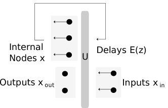
Figure 1: Schematic setup of the system. This network is described by Eq. (9). The $U$ in the figure represents a unitary component.

The transfer function of the given system can be formally solved as

$$x_{\mathrm{out}} =T(z)x_{\mathrm{in}}=\bigl{[}M_{3}E(z)\bigl{(}I-M_{1}E(z)\bigr{)}^{-1}M_{2}+M_{4}\bigr{]}x_{\mathrm{in}}$$ (9)

$$=\bigl{[}M_{3}\bigl{(}E(-z)-M_{1}\bigr{)}^{-1}M_{2}+M_{4}\bigr{]}x_{\mathrm{in}}.$$ (10)

Notice that this transfer function will have poles when

$$\det\bigl{(}I-M_{1}E(z)\bigr{)}=0.$$ (11)

We can define the zeros of this transfer function as $z$ satisfying $\det(T(z))=0$.

Throughout, we will also assume that the system is asymptotically stable. In terms of the network transfer function, all the eigenvalues of $M_{1}$ have norm less than $1$, with the consequence that $T(z)$ is bounded for $\Re(z)\geq 0$.

This transfer function has the important feature of being unitary whenever $z$ is purely imaginary. That is, $T(i\omega)T^{\dagger}(i\omega)=T^{\dagger}(i\omega)T(i\omega)=I$ whenever $\omega\in\mathbb{R}$. This is exactly the physical realizability condition for a passive linear system. We will refer to this constraint throughout the paper as the unitarity constraint. One consequence of this condition that can be obtained by analytic continuation is that $T(z)T^{\dagger}(-\overline{z})=I$ except when a pole is encountered.

Some observations. We see that the poles and zeros occur in pairs $z$, $-\overline{z}$. In this paper we will refer to such a pair as a zero-pole pair. In general, we observe that there may be infinitely many solutions to Eq. (11). If we take $M_{1}$ to be a real matrix, $z$ is a pole whenever $\overline{z}$ is also a pole. Furthermore, applying the maximum modulus principle shows the system is stable (see Appendix B). This implies that the poles appear in the left half-plane.

The solution to Eq. (11) can be found numerically within a bounded subset of $\mathbb{C}$. There are dedicated algorithms that use contour integration to guarantee finding all the roots within a contour, which we briefly discuss in Section 6.1. In the special case when the time delays are commensurate, we can re-write the equation for the poles as a polynomial equation of the variable $w=e^{-zT_{0}}$ for some $T_{0}$. Doing this will make the root finding procedure much more simple.

If the system has passive linear components other than delays and beamsplitters, the transfer function shown above may be modified. It will still have the same important features that the poles appear on the left half-plane (except when the system is marginally stable) and the function restricted to the imaginary axis is unitary.

4 Specific example and approximation procedure: one time delay and one beamsplitter

We will consider the example illustrated in Figure 2, where a single beamsplitter and time delay are combined to form a single-input and single-output (SISO) system. The example here is analogous to the one considered in Section VII B of [7].

Figure 2: A cavity formed by a single time delay $\tau$ and a single beamsplitter with reflectiveness $r$.

In this particular example, we use the convention that a beamsplitter has the transfer function

$$T_{BS}=\begin{pmatrix}t&-r\\ r&t\end{pmatrix},$$

where $r^{2}+t^{2}=1$, and a time delay of length $\tau$ has the transfer function

$$T_{\tau}(z)=e^{-\tau z}.$$

The transfer function of the system drawn in Figure 2 is given by

$$T(z)=\frac{e^{-\tau z}-r}{1-re^{-\tau z}}.$$ (12)

This transfer function is illustrated in Figure 3(a). The poles $p_{n}$ for $n\in\mathbb{Z}$ are found to be

$$p_{n}=\frac{1}{\tau}\bigl{(}\ln(r)+2\pi in\bigr{)}.$$ (13)

Notice that the real part is negative, as it should be for a stable system. Each of the poles in the system here corresponds to a cavity mode. The imaginary part corresponds to the mode frequency and the real part determines the linewidth properties. With this interpretation, we can readily relate the free spectral range to the delay length. In an attempt to approximate the system, we can consider a product of the following form of terms having the same (simple) poles as $T(z)$, satisfying the unitarity condition, and agreeing in value with $T(z)$ at $z=0$

$$\tilde{T}(z)=-\prod_{n\in\mathbb{Z}}c_{n}\biggl{(}\frac{z+\overline{p_{n}}}{z-p_{n}}\biggr{)}.$$ (14)

The factors $c_{n}$ are phases to ensure the convergence of the product. If we evaluate the product as a limit of products $\tilde{T}_{N}(z)$ as $N\to\infty$ such that for a fixed $N$, $\tilde{T}_{N}(z)$ is a product over $n=-N,-N+1,\ldots,N-1,N$, we can drop the $c_{n}$ factors by symmetry considerations.

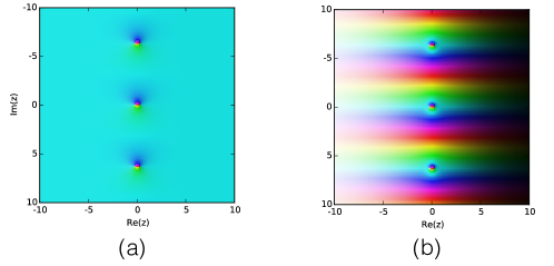
Figure 3: A comparison of two transfer functions as seen in the complex plane. The hue and the brightness correspond to the phase and magnitude, respectively. (a) The transfer function $T(z)=\frac{e^{-z}-r}{1-re^{-z}}$ corresponds to a cavity with $r=0.8$ and $\tau=1$. (b) The transfer function $T(z)=\frac{e^{-z}-r}{1-re^{-z}}e^{-z}$ in addition to a cavity augments a delay of length $\tau$ in sequence with the original cavity system.

One interpretation of each term in the product is the frequency-domain representation of a cavity mode. We can obtain an approximation for $T(z)$ by truncating the product with a finite number of poles. The resulting rational function can then be interpreted as the transfer function of a finite-dimensional system.

Notice that the procedure used to obtain $\tilde{T}(z)$ does not guarantee that $\tilde{T}(z)=T(z)$, although this is indeed the case for the example above. In general the procedure above may not capture some of the properties of the system. For example, if we added another delay with no feedback in sequence, we would obtain an additional phase factor dependent on $z$, while still satisfying the desired properties. For a SISO system satisfying the unitarity constraint with the same root-pole pairs, a phase dependence $T(z)=\tilde{T}(z)e^{-\alpha z}$ ($\alpha\geq 0$) is actually the most general modification we might need. For a system satisfying the same conditions but having $N$ input and output ports, the $e^{-\alpha z}$ term will be replaced by a similar singular function which we will refer to throughout as the singular term (see Section 5.1 for a discussion). An illustration of $T(z)$ and the transfer function resulting when an additional delay is augmented to the system is illustrated in Figure 3.

Notice how the augmented delay substantially changes some of the properties of the transfer function in the complex plane. For instance, when $\Re(z)\to-\infty$, the transfer function in Figure 3(a) approaches a constant, while that in Figure 3(b) diverges. In Section 8 we will be able to utilize the difference in behavior of transfer functions to determine whether they incorporate a nontrivial everywhere analytic term, like the exponential resulting from a time delay.

We can check to see if such a factor is needed in the factorization above. Assuming that $\lim_{\Re(z)\to-\infty}\tilde{T}(z)=C\neq 0$ (see Appendix E), we can take $\lim_{\Re(z)\to-\infty}T(z)$ to check if the additional phase factor is present in $T(z)$. We see $\lim_{\Re(z)\to-\infty}T(z)=-1/r$, which shows in our example that no such additional term is needed, and therefore $\tilde{T}(z)=T(z)$. It can be confirmed numerically that the values of $T(z)$ and $\tilde{T}(z)$ agree.

In the rest of the paper, we will show how a similar procedure can be applied more generally to multiple-input and multiple-output (MIMO) systems.

5 Factorization theorem and implications for passive linear systems

Certain kinds of matrix-valued functions can be factorized using the Potapov factorization theorem. A more general factorization theorem is discussed in Appendix C.2. Here we discuss a special case useful for our application. In Section 5.1 below we show how this special form can be obtained using the theorems in Appendix C.2.

theorem. Let $T(z)$ be a meromorphic matrix-valued function satisfying $T(z)T^{\dagger}(z)=I$ for $z\in i\mathbb{R}$ and bounded on the right half-plane $\mathbb{C}^{+}$. Then we can represent $T$ with the factorization

$$T(z)=UB(z)S(z),$$ (15)

where

$$B(z) =\prod_{k=1}^{\infty}B_{k}(z),\qquad S(z)=\overset{\curvearrowright}{\int_{0}^{\ell}}e^{-zK(t)\,dt}.$$ (16)

In the product, each of the terms $B_{k}$ has the form

$$B_{k}(z)=V_{k}\begin{pmatrix}e^{i\phi_{k}}\frac{z-\lambda_{k}}{z+\overline{\lambda_{k}}}I_{p_{k}^{\prime}{}}&0\\ 0&I\end{pmatrix}V_{k}^{-1}=I-P_{k}+A_{k}(z)P_{k}.$$ (17)

The $B_{k}$ terms are the Blaschke-Potapov factors written in the $s$-plane formalism (see Appendix A), and $U$ and the $V_{k}$’s are some unitary matrices. We use the symbol $\overset{\curvearrowright}{\int}$ to refer to the multiplicative integral, or product integral. The integral above is given by

$$S(z)=\lim_{\max\Delta t_{j}\to 0}e^{-zK(t_{0})(t_{1}-t_{0})}e^{-zK(t_{1})(t_{2}-t_{1})}\cdots e^{-zK(t_{n-1})(t_{n}-t_{n-1})},$$ (18)

where we take $0=t_{0}\leq t_{1}\leq\cdots\leq t_{n}=\ell$. In the integral, $K(t)$ is a summable non-negative family of Hermitian matrices with $\text{tr}[K(t)]=1$ on some interval $[0,\ell]$ for some $\ell$. The $P_{k}$ is an orthogonal projection, $A_{k}(z)=\frac{z-\lambda_{k}}{z+\overline{\lambda_{k}}}e^{i\phi_{k}}$, and $e^{i\phi_{k}}=\frac{|1-\lambda_{k}^{2}|}{1-\lambda_{k}^{2}}$ is a phase factor.

Notice that each Blaschke-Potapov factor has a zero at $\lambda_{k}$ and pole at $-\overline{\lambda_{k}}$. We will refer to the terms $B(z)$ and $S(z)$ above as the Potapov product and the singular term, respectively. Both $B(z)$ and $S(z)$ are inner functions. A function $F(z)$ is said to be inner if it satisfies the unitarity condition $F(z)F(z)^{\dagger}=I$ for $z\in i\mathbb{R}$ and is contractive on the right half-plane (i.e. $F(z)F^{\dagger}(z)\leq I$ for $z\in\mathbb{C}^{+}$). When $B(z)$ is a finite product, the $V_{k}$ terms can be redefined so that the phase factors $\phi_{k}$ can be absorbed into the unitary matrix $U$.

5.1 Obtaining the special case of the factorization theorem for passive systems

In this section, we will show how the theorems in Appendix C.2 are used to obtain the special form we will use.

First, notice we assumed above that $T(z)$ is a meromorphic matrix-valued function unitary for $z\in i\mathbb{R}$ and bounded on $\mathbb{C}^{+}$. These assumptions hold for the system described in Section 3. By Appendix B, it follows that $T(z)$ is an inner function on $\mathbb{C}^{+}$.

We are now in a position to apply the Potapov factorization theorem stated in Appendix C.2. Setting $J=I$ in the theorem and applying the Cayley transformation (discussed in Appendix A) to map the unit disc in the theorem to the right half-plane, the theorem implies that $T(z)$ has the form

$$\bar{B}_{\infty}(z)\bar{B}_{0}(z)S(z),$$ (19)

where $\bar{B}_{i}(z)=B_{i}(\frac{z-1}{z+1})$ for $i=0,\infty$ and $S(z)$ results from a similar transformation on the multiplicative integral in Eq. (48). We will only need to write the expression for $\bar{B}_{0}(z)$ explicitly. After some algebra due to changing the domain from $\mathbb{D}$ to $\mathbb{C}^{+}$, one obtains the form in Eq. (17).

Because $T(z)$ has no poles on $\mathbb{C}^{+}$, the term $\bar{B}_{\infty}(z)$ is trivial. Notice that $S(z)$ resulting in our discussion may only have poles only for $z\in i\mathbb{R}$, because of the form of the integrand of the multiplicative integral of the Potapov factorization.

$T(z)$ has no poles for $z\in i\mathbb{R}$. Therefore $S(z)$ is analytic everywhere. The term $S(z)$ is unitary for $z\in i\mathbb{R}$ since $\bar{B}_{0}(z)$ and $T(z)$ are also unitary for $z\in i\mathbb{R}$. We also note that $S(z)$ is contractive on $\mathbb{C}^{+}$, and refer the reader to Potapov’s paper [19] for details (in particular, notice detaching single Blaschke-Potapov term from a contractive function with the same zero results in a contractive function). Since $S(z)$ is an entire contractive function unitary on $i\mathbb{R}$, we can apply the second theorem from Appendix C.2, giving the expression in Eq. (51),

$$S(z)=S(0)\overset{\curvearrowright}{\int_{0}^{\ell}}e^{-zK(t)\,dt}.$$ (20)

If we wish, we can re-define the $V_{k}$ terms in $\bar{B}_{0}(z)$ so that $\bar{B}_{0}(z)S(0)S(z)=U\tilde{B}_{0}(z)S(z)$ (the convergence criterion depends only on the zeros of the product). Finally, we drop the tilde to obtain the form $T(z)=UB(z)S(z)$ in Eq. (15).

5.2 Interpretation as cascaded passive linear network

We remark that the Blaschke-Potapov factorization of an inner function can be interpreted as a limiting case of a system of beamsplitters, feedforward delays, and cavity modes.

First, we will interpret the Blaschke-Potapov product in the optical setting. Each unitary matrix appearing in the factorization can be interpreted as a generalized beamsplitter. Each Blaschke factor with zero $\lambda_{k}$ has the form $B_{k}(z)$ of Eq. (17) in Section 5.1. We can interpret $A_{k}(z)$ in Eq. (17) as the transfer function of a single cavity mode. The location of the zero $\lambda_{k}$ in the complex plane determines the detuning and linewidth of the mode. The modes resulting from the Blaschke-Potapov product can be visualized as a sequence of components of the form portrayed in Figure 4.

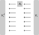
Figure 4: A physical interpretation of a single Blaschke-Potapov term. Here the $V_{k}$ represents a beamsplitter and the $A_{k}$ represents a passive SISO system with a single degree of freedom. The zero-pole interpolation generates a series of factors of this form in a cascade.

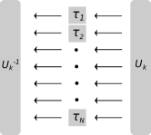
Figure 5: A physical interpretation of a component resulting in an approximation of the multiplicative integral. Here the $U_{k}$ represents a beamsplitter and each $\tau_{j}$ ($j=1,\ldots,N$) represents a delay of that duration.

Next, we shall interpret the singular term represented as the multiplicative integral in Eq. (18) of Section 5. Approximating the multiplicative integral over intervals $\Delta t_{k}=t_{k+1}-t_{k}$, we obtain a product of terms that can each be represented by

$$e^{-zK(t_{k})(t_{k+1}-t_{k})}=e^{-zK(t_{k})\Delta t_{k}}=U_{k}e^{-zD_{k}}U_{k}^{\dagger}.$$ (21)

Here $K(t_{k})\Delta t_{k}\geq 0$ and $U_{k}$ are some unitary matrices resulting in the diagonalization $K(t_{k})\Delta t_{k}=U_{k}D_{k}U_{k}^{\dagger}$. Each term of the form (21) can be interpreted as a component consisting of parallel feedforward delays inserted between two unitary components as illustrated in Figure 5. The sum of the delays across the parallel ports for each such term is given by $\text{tr}(K(t_{k})\Delta(t_{k}))=\Delta t_{k}$. It is possible to further approximate the feedforward delays in the factorization with modes, but we will refrain from doing this here for conceptual clarity

6 Approximation Procedure – Zero-Pole Interpolation

In order to reconstruct an approximation for the transfer function $T(z)$ using only a finite number of modes, we will use a two-step procedure. The first step consists of finding the zero-pole pairs in a region of interest. The second step consists of examining the numerical values of the transfer function near the zeros or poles to obtain the correct form of each of the Blaschke-Potapov terms, which are determined up to a constant unitary factor. The product of the resulting terms will equal a truncated version of the Blaschke-Potapov product discussed in Section 5.1, and will approximate the transfer function in the region of interest.

We will take a transfer function $T$ and obtain an $M$-dimensional approximation by identifying appropriate factors for a Blaschke-Potapov product. It is possible that the transfer function may have a nontrivial singular component (i.e. a nontrivial everywhere analytic term) as discussed in Section 5.1, in which case the zero-pole interpolation may not reproduce a converging sequence of approximations to the given transfer function $T(z)$. In this section we assume that the singular term is trivial or otherwise unimportant. In any case we determine $U$ in Eq. (15) of Section 5.1 using $T(0)$.

A trivial example when the above approach might fail is a delay with no feedback at all. In this case, there are no poles to evaluate and the method fails. When a transfer function is entirely singular, or when its singular component cannot be neglected, a different approach will be needed, such as using the Padé approximation. This is discussed in Appendix D.

6.1 Identifying mode location

We remind the reader that we take our coordinate system in the $s$-domain. We assume for simplicity that we are interested in the behavior of the system near the origin. However, our procedure can be used to obtain approximations of the given transfer function for arbitrary regions in the $s$-plane. In order to identify the appropriate modes, we find roots of the transfer function of the full system, $\lambda_{1},\ldots,\lambda_{M}$ (with corresponding poles $p_{1},\ldots,p_{M}$). Each root will represent a “trapped” resonant mode. In general, there will be infinitely many such roots in the full system, so it is important to have a criterion for selecting a finite number of roots. Each root will have an imaginary part, which will correspond to the frequency of the mode, and a real part, which is linked to the linewidth of the mode. One criterion might be to select root whose imaginary part falls in some range $[-\omega_{\max},\omega_{\max}]$, so that the approximation is valid for a particular bandwidth. This approximating system may be improved by increasing the maximum frequency, $\omega_{\max}$. As the number of zero-pole pairs increases, the quality of the approximation increases, but in addition the approximated system will incur a greater number of degrees of freedom.

Luckily there is a well-known technique that can be used based on contour integration developed in [2]. This algorithm runs in a reasonable time and can essentially guarantee that it does indeed find all of the desired points. The latter point is an important feature that most typical root-finding algorithms do not have because they do not utilize the properties of analytic functions. For details about a more polished algorithm see [11]. Methods of this kind require a contour in the complex plane as the input in which the roots of the function will be found. This contour may be, for example, a rectangle in the complex plane. In practice we may make use of symmetries in the system and the known regions where poles and zeros are located.

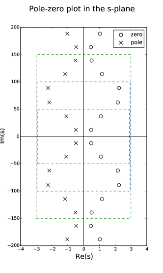
Figure 6: Sketch of root-finding procedure. This plot illustrates the locations where root-pole pairs may be found. As the contours grow and includes more root-pole pairs, the quality of the approximation improves. The plot in this figure is based on Example 2 from Section 7.2.

In Figure 6 we illustrate the step of our procedure for finding roots or poles. The various contours in dashed lines represent areas where roots and poles will be found. Notice in this plot that the roots and poles lie along a strip close to the imaginary axis. This is a typical feature of highly resonant systems (i.e. effective cavity modes have a long lifetime) since the real part of each pole in the system corresponds to the exponent of decay of each mode. The system illustrated Figure 6 originates from Example 2 in Section 7.2. If the maximum possible real part of each root is determined for the system of interest, a computational advantage can be gained since the contour does not need to be extended beyond that value.

6.2 Finding the Potapov projectors

The procedure we use assumes that the given transfer function $T(z)$ has a specific form guaranteed by the factorization theorem (see Eq. (15) in Section 5.1). For the purposes of this section, we neglect the contribution due to the singular term (the $S(z)$ in Eq. (15)). This procedure is similar to the zero-pole interpolation discussed in [1]. We handle the singular term separately, as we will discuss in Section 8.

We introduce an inductive procedure for this purpose. Each step will involve extracting a single factor of the Blaschke-Potapov product. We suppose the full transfer function being approximated is $T(z)$, and that it has a pole at $p$. Based on the form of the Blaschke-Potapov factors, we can separate the transfer function into the product

$$T(z)=\tilde{T}(z)\biggl{(}I-P+P\biggl{(}\frac{z+\overline{p}}{z-p}\biggr{)}\biggr{)}.$$ (22)

The $P$ is in general the orthogonal projection matrix onto the subspace where the multiplication by the Blaschke factor takes place. We wish to extract the $P$ given the known location of the pole $p$, which we assume to be a first-order pole for simplicity. We also assume for simplicity that $P$ is a rank one projection, and so it can be written as the product of a normalized vector

$$P=vv^{\dagger}.$$

The simplifying assumptions above have been sufficient for the systems we inspected, and could be easily removed. Rewriting, we obtain the relationship

$$T(z)(z-p)=(z-p)\tilde{T}(z)(I-P)+({z+\overline{p}})\tilde{T}(z)vv^{\dagger}.$$ (23)

Now take $z\to p$. We assumed that $T(z)$ has a first-order pole at $p$, so $\tilde{T}(z)$ will be analytic at $p$. Therefore, the first term on the right hand side goes to zero. Taking $L\equiv\lim_{z\to p}T(z)\*(z-p)$, we get

$$L=({p+\overline{p}})\tilde{T}(p)vv^{\dagger}.$$ (24)

Since we assumed that $P$ is a rank one projector, have obtained an expression where $L$ must also be rank one. In order to find $v$ we can simply find the normalized eigenvector corresponding to the nonzero eigenvalue of $L$. This task may be done numerically. Finally, we can find the $\tilde{T}(z)$ from Eq. (22) above.

The procedure outlined above may be repeated for each of the $M$ desired roots of $T(z)$ to obtain a factorization

$$T(z)=T_{M}(z)\prod_{k=1}^{M}\biggl{(}I-P_{k}+P_{k}\biggl{(}\frac{z+\overline{p}_{k}}{z-p_{k}}\biggr{)}\biggr{)}.$$ (25)

We assume that the $T_{M}(z)$ is close to a constant in the region of interest. This is exactly true in the case where the transfer function $T$ has only the $M$ roots picked. We can approximate $T_{M}$ with a unitary factor that can be determined from $T$ and the product in Eq. (25) evaluated at some point $z_{0}$ in the region of interest.

The computer code for this procedure can be found on [22].

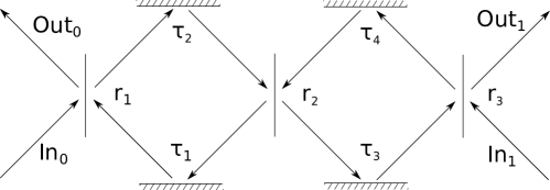
Figure 7: The network of Example 1 in Section 7.1. For this network the zero-pole interpolation produces accurate approximating functions because the singular term is trivial.

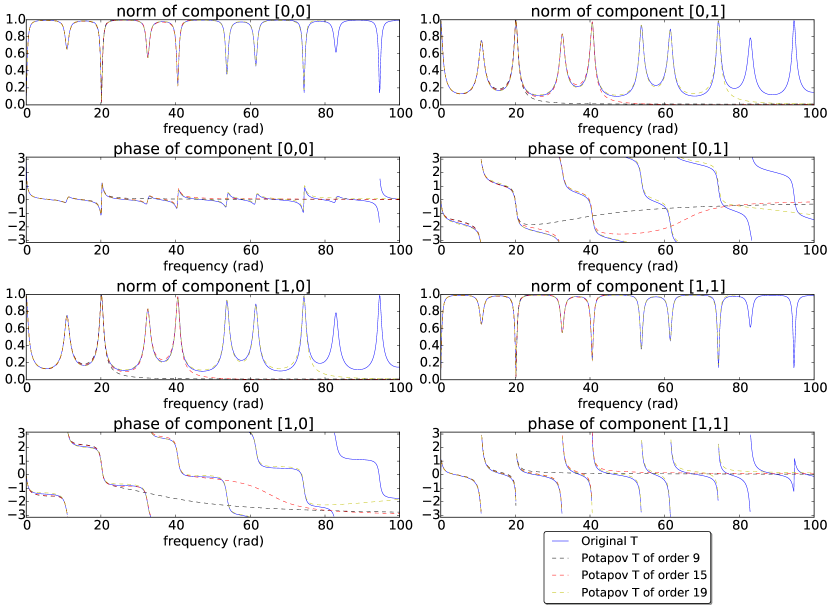
Figure 8: A plot of the transfer function $T$ of Example 1 from Section 7.1 and various approximated transfer functions generated by the zero-pole interpolation method. We illustrate the components of $T(i\omega)$ for $\omega\geq 0$. We only include nonnegative $\omega$ because of the symmetry of both $T$ and its approximations. The zero-pole interpolation appears to converge to the correct transfer function as we add more terms.

7 Examples of zero-pole decomposition

In this section, we show two examples where we have applied the zero-pole procedure. The networks used for these examples are shown in Figures 7 and 9. We plot the various components of the transfer functions of these networks along $i\omega$ for $\omega\geq 0$ in Figures 8 and 10, respectively. Along both examples, we also plot several approximate transfer functions determined by the zero-pole interpolation of Section 6. The approximate transfer functions correspond to a Blaschke-Potapov product that has been truncated to a certain order. In both examples we see that as we increase the number of terms, the approximation improves. The first example illustrates the case when the zero-pole interpolation converges to the correct transfer function. In the second example, while the zero-pole interpolation appears to converge, the function to which it converges deviates from the original transfer function. This suggests that the singular term $S(z)$ in Section 5.1 makes a contribution for which the zero-pole interpolation does not account. In Section 8, we discuss a condition for convergence and show how the effects of the singular term may be separated from the rest of the system. Figure 10 also includes the transfer function once the singular term has been removed, demonstrating that the zero-pole approximations converge to that function.

7.1 Example 1. Zero-pole interpolation converges to given transfer function

The first example we discuss involves two inputs and two outputs. Figure 7 shows this network explicitly. In Figure 8 we see that the zero-pole interpolation appears to converge to the correct transfer function. We can check this by confirming that the $M_{1}$ is nonsingular, as we will show in Section 8.

The matrices of Eq. (8) in Section 3 are given by

$$M_{1}=\begin{bmatrix}0&-r_{1}&0&0\\ -r_{2}&0&t_{2}&0\\ 0&0&0&-r_{3}\\ t_{2}&0&r_{2}&0\end{bmatrix},\qquad M_{2}=\begin{bmatrix}t_{1}&0\\ 0&0\\ 0&t_{3}\\ 0&0\end{bmatrix},$$ (26)

$$M_{3}=\begin{bmatrix}0&t_{1}&0&0\\ 0&0&0&t_{3}\end{bmatrix},\qquad M_{4}=\begin{bmatrix}r_{1}&0\\ 0&r_{3}\end{bmatrix}.$$ (28)

Here $\tau_{1}=0.1$, $\tau_{2}=0.23$, $\tau_{3}=0.1$, $\tau_{4}=0.17$, $r_{1}=0.9$, $r_{2}=0.4$, $r_{3}=0.8$.

7.2 Example 2. Zero-pole interpolation fails to converge to given transfer function

In the next example, we have two inputs and two outputs, as in the first example of Section 7.1. However, the design of the network is significantly different. The network for this example is shown in Figure 9. This example combines elements of an interferometer and an optical cavity. In some regimes, such as $\tau_{4}\ll\tau_{2}$, the zero-pole decomposition yields a good approximation for the transfer function. In general, however, the singular component of the transfer function must be incorporated in some other way.

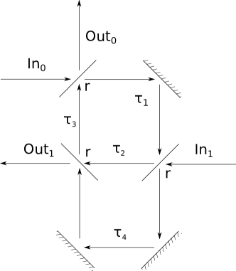
Figure 9: The network of Example 2 in Section 7.2. In this network the zero-pole interpolation method would not be wholly applicable because the singular term is nontrivial.

The matrices of Eq. (8) in Section 3 are given by

$$M_{1}=\begin{bmatrix}0&0&-r&0\\ r&0&0&0\\ 0&r&0&t\\ t&0&0&0\end{bmatrix},\qquad M_{2}=\begin{bmatrix}t&0\\ 0&t\\ 0&0\\ 0&-r\end{bmatrix},$$ (29)

$$M_{3}=\begin{bmatrix}0&0&t&0\\ 0&t&0&-r\end{bmatrix},\qquad M_{4}=\begin{bmatrix}r&0\\ 0&0\end{bmatrix}.$$ (31)

Here $\tau_{1}=0.1$, $\tau_{2}=0.039$, $\tau_{3}=0.11$, $\tau_{4}=0.08$, $r=0.9$.

The important differentiating feature from the previous example of Section 7.1 is that the singular term for the transfer function of this network is nontrivial. This can be seen when examining the resulting transfer functions from the zero-pole interpolation, which are shown in Figure 10. In Section 8 we will show that this condition can be checked by observing that the $M_{1}$ in Eq. (29) is singular.

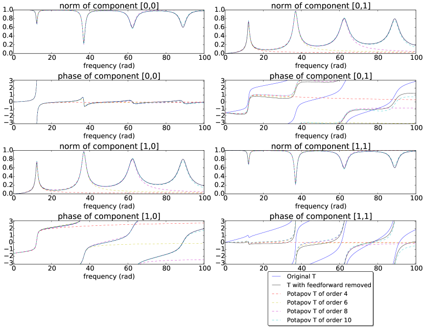
Figure 10: A plot of the transfer function $T$ of Example 2 from Section 7.2 and various approximated transfer functions generated by the zero-pole interpolation method. We also include the transfer function resulting when the singular term is removed, to which the approximated functions converge. We illustrate the components of $T(i\omega)$ for $\omega\geq 0$. We only include nonnegative $\omega$ because of the symmetry of both $T$ and its approximations. See Section 7.2 for further details.

In Figure 10, we see that the zero-pole interpolated transfer functions deviate from the true transfer function in the $(0,1)$ and $(1,1)$ phase components. This demonstrates how in general it is important to consider the singular function. On the other hand, for the systems in consideration it is possible to separate the Blaschke-Potapov product from the singular term, which corresponds to feedforward-only components, as discussed in Section 8.3. In black we graph the transfer function components resulting once the feedforward-only components have been removed. Up to a unitary factor, this function is equal to the infinite Potapov product. We see that the approximated transfer functions from the zero-pole interpolation converge to this function.

8 The Singular Term

In this section, we examine the factorization of the transfer function given in Eq. (15) in Section 5.1. In the form of the fundamental theorem by Potapov that we obtained, we had an infinite product of Blaschke-Potapov factors and a singular term. Although the zero-pole decomposition allowed us to extract the Blaschke-Potapov factors, it gave us no information regarding the singular term. In some systems, it may be crucial to include the singular term to obtain a good approximation of the system. To learn about this term, we will need a different method.

In this section, we give a condition for the singular term to be trivial. This condition can then be specialized to the network from Section 3. Based on this condition, we can develop a method to explicitly separate the network described by Eq. (8) in Section 3 into the Potapov product and the singular term.

8.1 Condition for the multiplicative integral term to be trivial

We examine the form of the singular term in the factorization theorem and notice that its determinant becomes large when $\Re(z)\to-\infty$. To avoid mathematical details, we will assume here that the Blaschke-Potapov product $\prod B_{k}(z)$ is well-behaved in the limit $\Re(z)\to-\infty$ in the sense that the limit of the product converges (to a nonzero constant). Justification for this assumption is discussed further in Appendix E. We have the following observations.

Observation. If $\lim_{\Re(z)\to-\infty}T(z)$ is a constant, then the multiplicative integral in Eq. (15) of Section 5.1 is a constant.

This follows from the properties of the multiplicative integral defined in Eq. (47) of Appendix C.1.

Observation. In particular, for the transfer function $T(z)$ in Eq. (9) of Section 3, $\lim_{\Re(z)\to-\infty}T(z)$ is a constant if and only if $M_{1}$ in Eq. (9) is full-rank. This gives a sufficient condition for when the zero-pole expansion converges exactly.

To obtain this result, it is enough to consider the term $(E(-z)-M_{1})^{-1}$ in the limit $\Re(z)\to-\infty$.

The above observations can be seen in the two examples discussed in Section 7. In Example 1, the $M_{1}$ matrix is full-rank, while in Example 2 it is not.

8.2 Maximum contribution of singular term

For many applications we anticipate that we may be able to drop the contribution of the singular term altogether. One example is an optical cavity in certain regimes. If the lifetime of the modes in the cavity is long in comparison to the delays in the system, we would expect the delays to be less significant. We would like to be able to provide a justification for when it is acceptable to neglect the singular term.

First, we will obtain the maximum value for $\ell$ necessary in the multiplicative integral appearing in Eq. (16) of Section 5.1. This is an important result because it tells us that the lengths of the delays themselves determines the greatest contribution of the singular function.

Remark. To apply the factorization in Eq. (15) of Section 5.1 to the transfer function in Eq. (9) of Section 3, it suffices to take $\ell\leq\sum_{k}T_{k}$.

This can be seen by noting the scaling of $\det[(E(-z)-M_{1})^{-1}]$ in the limit $\Re(z)\to-\infty$.

The above bound occurs in the case of several delays feeding forward in sequence.

We can give one condition under which the singular term can be dropped: $|z|\ll 1/\ell$. Furthermore, crude estimates for the error can now be found using the Taylor expansion of the exponential.

Intuitively, Potapov factors correspond to resonant modes while the singular function corresponds to feedforward-only components. With this interpretation, we see that the zero-pole interpolation yields a transfer function close to the true transfer function when the feedforward-only term can be neglected. We can interpret $\ell$ as an upper bound on the duration of time the signal can spend being fed-forward only. When $1/\ell$ becomes large with respect to the size of the region of interest in the frequency domain, the feedforward-only terms become unimportant.

8.3 Separation of the Potapov product and the singular term in an example

In this section, we discuss how for a network of beamsplitters and delays the Blaschke-Potapov product and the singular term of Section 5.1 can be separated explicitly. We will give a systematic procedure at least with the simplifying assumption that the delays are commensurate (are rational multiples of one another). In practice, one can always approximate the delays to arbitrary precision with commensurate delays, resulting in a large but sparse network.

To intuitively motivate the procedure we will use, we first give a demonstration for the case of the example in Section 7.2. In this network, extracting a single feedforward delay is sufficient for obtaining the separation of the two terms we desire. We will assume that $\tau_{2}<\tau_{4}$. The important observation is that a collection of $k$ parallel delays can be commuted with a given a unitary component $U$ of $k$ ports. This is illustrated in Figure 11(a).

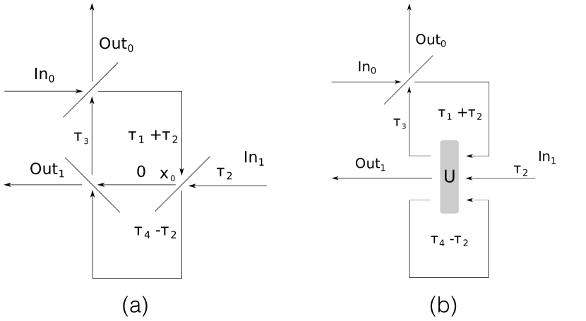
Figure 11: An illustration of one way the Potapov product and the singular function can be separated for Example 2 in Section 7.2. We notice that some of the parallel delays can be commuted with a beamsplitter, forming the network in (a). The node labeled $x_{0}$ can then be eliminated, forming the network in (b) which now has a 3-input 3-output unitary component denoted by $U$.

Next, it becomes apparent in the new network shown in Figure 11(a) that one of the internal system nodes is unnecessary, since it is followed by a delay of duration zero (call it $x_{0}$). For this reason, $x_{0}$ can be eliminated from the network. In the process, we can combine two of the unitary components preceding and following $x_{0}$ to form a separate unitary component, illustrated in Figure 11(b). The network depicted in Figure 11(b) can be decomposed into a feedforward-only component followed by a network for which the $M_{1}$ matrix is invertible. The feedforward-only component consists of the identity applied to $\operatorname{In}_{0}$ combined in parallel with the addition of the delay $\tau_{2}$ to $\operatorname{In}_{1}$ - that is, the feedforward component only delays the input from port $\operatorname{In}_{1}$ by $\tau_{2}$. The network following the feedback-only component results from the exclusion of the delay $\tau_{2}$ in Figure 11(b). Since its $M_{1}$ matrix is invertible, this network has trivial singular part.

8.4 Systematic separation of Potapov product and analytic term for passive delay networks

Suppose we have a system given in the form of Eq. (8) in Section 3. Our observation that in order for the multiplicative integral term to be trivial we need $M_{1}$ to be invertible suggests that there may be a way to isolate the Potapov product term from the remaining analytic function. We now present a systematic way of doing this. For simplicity we will assume that all the delays are comensurate. Without a loss of generality, we can write the system in such a way that all the delays have equal duration, and therefore $E(z)$ is a multiple of the identity.

The essential idea is to make a change of basis that allows the elimination of a node at the expense of modifying the inputs in such a way that a part of the analytic term can be extracted from the network. We are interested in the case with $M_{1}$ not invertible. When this is the case, we can find some change of basis represented by the matrix $S$ such that

$$M_{1}=SJS^{-1},$$ (32)

where the $J$ is the Jordan decomposition of $M_{1}$ such that the zero eigenvalue block is at the right bottom block of $J$. We introduce $\bar{x}=S^{-1}x$ and rewrite the equation for $x$ in Eq. (9) of Section 3 as

$$\bar{x}=JS^{-1}E(z)S\bar{x}+S^{-1}M_{2}x_{\mathrm{in}}.$$ (33)

Now, $\bar{x}_{1}=[S^{-1}M_{2}x_{\mathrm{in}}]_{1}$, which depends only on the inputs. The subscript here refers to the first component. We can separate the dependence of the remaining coordinates of $\bar{x}$. Denoting the last column of $S$ by $S_{1}$, the matrix of columns excluding the last as $S_{\setminus 1}$, and the matrix of rows of $J$ excluding the last as $J_{/1}$, we can write

$$\bar{x}_{\setminus 1}=J_{/1}S^{-1}E(z)[S_{1}\bar{x}_{1}+S_{\setminus 1}\bar{x}_{\setminus 1}]+S^{-1}M_{2}x_{\mathrm{in}}.$$ (34)

We can now separate the network into two networks. The first network takes the original inputs $x_{\mathrm{in}}$ and yields the outputs

$$\tilde{x}_{\mathrm{in}}=J_{/1}S^{-1}E(z)S_{1}\bigl{[}S^{-1}M_{2}x_{\mathrm{in}}\bigr{]}+S^{-1}M_{2}x_{\mathrm{in}}.$$ (35)

Notice the first network is a feedforward network (i.e. no signal feeds back to a node from which it originated). The second network takes the $\tilde{x}_{\mathrm{in}}$ as inputs and yields the outputs

$$\bar{x}_{\setminus 1}=J_{/1}S^{-1}E(z)S_{\setminus 1}\bar{x}_{\setminus 1}+\tilde{x}_{\mathrm{in}}.$$ (36)

Using the simplifying assumption that the $E(z)=Ie(z)$ is a multiple of the identity, we obtain

$$\bar{x}_{\setminus 1}=\tilde{J}e(z)\bar{x}_{\setminus 1}+\tilde{x}_{\mathrm{in}},$$ (37)

where the $\tilde{J}$ is matrix resulting from dropping the last row and column in $J$. We see that Eq. (37) has the same form to the original equation for $x$ in Eq. (9) in Section 3. The difference is that now the $\tilde{J}$ replaces $M_{1}$, and has one fewer zero eigenvalue. Conveniently, $\tilde{J}$ is also in its Jordan normal form, so the procedure can be repeated until the matrix ultimately replacing $M_{1}$ (call it $\tilde{M}_{1}$) has no zero eigenvalues left. In this case $\tilde{M}_{1}$ is an invertible matrix, which is exactly the condition we needed for the transfer function of the network to consist of only the Potapov product and not the multiplicative integral.

A very simple example illustrating the intuition of our procedure is a network where the internal nodes all feed forward in sequence. Explicitly, take

$$M_{1}=\begin{pmatrix}0&1&0&0\\ 0&0&1&0\\ 0&0&0&1\\ 0&0&0&0\end{pmatrix}.$$ (38)

Notice that this matrix is already in its Jordan-canonical form, so the analysis becomes transparent. Also notice that all of the eigenvalues of $M_{1}$ are zero, which implies that our procedure will extract all the delays and collect them in the singular term.

9 Relationship to the ABCD and SLH formalisms

In this section we demonstrate how the approximating system our procedure designs is physically realizable. In particular we show how to extract the ABCD and SLH forms for a single term resulting in the truncated Blaschke-Potapov product designed to approximate the transfer function of the system. Since the transfer function is equal to a product of such terms, we can interpret the approximating system as a sequential cascade of single-term elements of this form.

The state-space representation of the Potapov factor will have the form

$$B(z)=C(Iz-A)^{-1}B+D.$$ (39)

To obtain the ABCD model for a single Potapov factor, begin with the following factor

$$B(z)=I-vv^{\dagger}+vv^{\dagger}\biggl{(}\frac{z+\overline{\lambda}}{z-\lambda}\biggr{)}=I+vv^{\dagger}\frac{\lambda+\overline{\lambda}}{z-\lambda}.$$ (40)

In this instance we have also assumed that the orthogonal projector $P=vv^{\dagger}$ has rank one.

There is some freedom in how the $B$ and $C$ matrices may be chosen. In particular, one choice is also consistent with the form used for passive components in the SLH formalism. The ABCD formalism is related to the SLH formalism in the following way for a passive linear system.

$$A=-\frac{1}{2}C^{\dagger}C-i\Omega,\qquad B=-C^{\dagger}S,\qquad D=S.$$ (41)

In order to satisfy the above equations, we choose

$$B=-\sqrt{-(\lambda+\overline{\lambda})}v^{\dagger},\qquad C=\sqrt{-(\lambda+\overline{\lambda})}v.$$ (42)

Finally, we can solve for the $\Omega$.

$$\Omega=\biggl{[}i\biggl{(}A-\frac{1}{2}(\lambda+\overline{\lambda})\biggr{)}\biggr{]}=-\bigl{[}\Im(A)\bigr{]}.$$ (43)

For the last equality, we use that $\frac{1}{2}(\lambda+\overline{\lambda})$ is exactly the real part of the eigenvalue, and so cancels exactly with the real part of $A$. The only remaining component is the imaginary part of $A$, which is multiplied by $i$. Notice the $\Omega$ satisfies the condition of being Hermitian.

10 Simulations in Time Domain

We translate our model into the ABCD state-space formalism, as discussed in Section 9. Doing this allows us to run a simulation in the time domain. Notice that for linear systems this approach suffices for finding the dynamics in the time domain. We can apply an input field at some frequency and record the output. The relationship between the inputs and outputs at the steady-state will correspond to the value of the transfer function at the appropriate frequency.

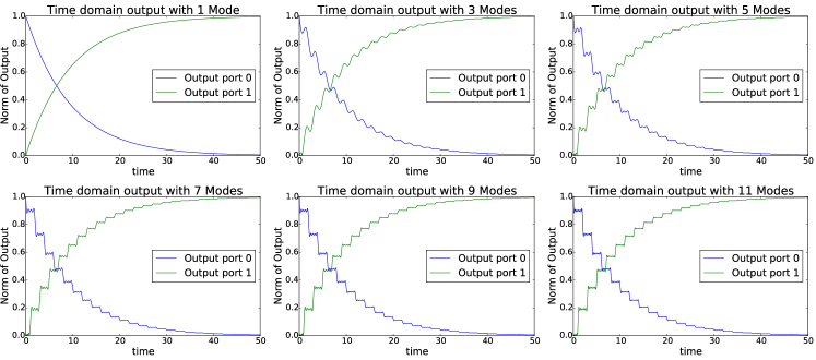
Figure 12: The output from a Fabry-Pérot cavity with initial state zero. The mirror has reflectivity $r=0.9$ and the duration of the delay is $1$. The two output ports represent the signal reflected and the signal transmitted through the cavity. The signal enters the system from port $0$ and exists from both ports $0$ and $1$ (see Figure 13). In steady-state, the norm of output $0$ converges to zero, an the norm of output $1$ converges to $1$. The stated number of modes in each diagram is the number of modes used in the delay. We see that adding more modes eventually converges to a piecewise step function. The steps result from the round-trip of the signal inside the cavity.

Figure 13: Interpretation of transient dynamics of the system in the Fabry-Pérot cavity considered. Before the system achieves steady-state, we can learn about the output by tracing the possible paths the signal may follow. The arrows in the diagram between the two mirrors represent the possible paths the signal may follow before leaving through an output port. We use the vertical direction to represent time. For each arrow in each output direction, some of the signal leaves through one of the mirrors. We will therefore see a step in the output as a function of time. This gives a physical interpretation of the steps seen in Figure 12.

As a simple example, we consider the input-output relationship of a Fabry-Pérot cavity with a constant input (i.e. $\omega=0$) at one of the ports (port $0$) and zero input in the other port (port $1$). In the steady-state, the signal will be transmitted from the input port $0$ to the output port $1$. However, if the initial state of the system is different than the steady-state, we will observe some transient behavior in the system. This transient behavior is captured by our simulation and is demonstrated in Figure 12. Here, we show the outputs of the two ports based on different numbers of modes selected to approximate the cavity formed due to the delay. As the number of modes is increased, we see the signal from the output ports as a function of time approaches a step function, and we better reproduce the time-domain dynamics of the network with feedback loops. The jumps we see in the time-domain correspond physically to times when a propagating signal arrives at one of the ports. This physical interpretation is further explained in Figure 13.

11 Conclusion

In this paper we have utilized the Blaschke-Potapov factorization for contractive matrix-valued functions to devise a procedure for obtaining an approximation for the transfer function of physically realizable passive linear systems consisting of a network of passive components and time delays. The factorization in our case of interest consists of two inner functions - the Blaschke-Potapov product, a function of a particular form having the same zeros and poles as the original transfer function, and an inner function having no roots or poles (a singular function). The factors in the Potapov product correspond physically to resonant modes formed in the system due to feedback, while the singular term corresponds physically to a feedforward-only component. We also demonstrate how these two components may be separated for the type of system considered.

The transfer function resulting from our approximation can be used to obtain a finite-dimensional state-space representation approximating the original system for a particular range of frequencies. The approximated transfer function can also be used to obtain a physically realizable component in the SLH framework used in quantum optics. Our approach has the advantage that the zero-pole pairs corresponding to resonant modes are identified explicitly. In contrast, obtaining a similar approximation for a feedforward-only component requires introducing spurious zeros and poles. Our approach has the advantages that we may retain the numerical values of the zero-pole pairs of the original transfer function in our approximated transfer function and that we can conceptually separate these zero-pole pairs from spurious zeros and poles. These advantages may be important in applications and extensions of this work.

We hope that in the future our factorization procedure may be extended to a more general class of linear systems. We also hope to introduce nonlinear degrees of freedom in a similar way to atoms in the Jaynes-Cummings model and quantum optomechanical devices in the presence of modes formed due to optical cavities.

Appendix A The Cayley Transform

Throughout this paper, we work in the frequency domain $\mathbb{C}$ common in the engineering literature, where the imaginary axis takes values $i\omega$. In some of the literature, a domain related by a bijective conformal transformation is used instead. The imaginary axis is mapped to the unit circle, and the right half-plane $\mathbb{C}^{+}$ is mapped to the unit disk $\mathbb{D}$. This mapping is known as the Cayley transform, and the two domains are often called the $s$-domain and $z$-domain, respectively.

The mapping from $\mathbb{C}^{+}$ to $\mathbb{D}$ is given by

$$f(z)=\frac{z-1}{z+1}.$$

The mapping from $\mathbb{D}$ to $\mathbb{C}^{+}$ is given by

$$f^{-1}(z)=\frac{1+z}{1-z}.$$

Sometimes in the literature the upper half-plane is used instead of the right half-plane, which slightly changes the transformation.

In our notation, a zero $z_{k}$ of the Blaschke factor in the disc $\frac{z_{k}-z}{1-\overline{z_{k}}z}\frac{|z_{k}|}{z_{k}}$ is transformed to a zero in the plane $\lambda_{k}=\frac{1+{z_{k}}}{1-{z_{k}}}$ of the factor $e^{i\phi_{k}}\frac{z-{\lambda_{k}}}{z+\overline{\lambda_{k}}}$, where $e^{i\phi_{k}}=\frac{|1-\lambda_{k}^{2}|}{1-\lambda_{k}^{2}}$ contributes only a phase.

Appendix B Unitarity implies a function is inner

(Based on [3], Lemma 3 on page 223.)

This section will prove the assertion that

$$T(z)T^{\dagger}(z)=I\quad\text{for }z\in i\mathbb{R}\quad\implies\quad T(z)T^{\dagger}(z)\leq I\quad\text{for }z\in\mathbb{C}^{+},$$ (44)

assuming $T(z)$ is an $N\times N$ matrix-valued analytic (except possibly at infinity) function bounded in $\mathbb{C}^{+}$.

For any appropriately sized unit vectors ${u}$, ${v}$, we have from the Cauchy-Schwartz inequality and the maximum modulus principle that

$$\bigl{|}\bigl{\langle}u,T(z)v\bigr{\rangle}\bigr{|}^{2}\leq\|u\|\bigl{\|}T(z)v\bigr{\|}\leq 1.$$ (45)

Since the $u$, $v$ were arbitrary, the assertion follows.

Appendix C Potapov factorization theorem and non-passive linear systems

In this section we cite the Potapov factorization theorem for $J$-contractive matrices. This factorization, when applicable, consists of several terms which each have a different property. For this paper we will only need a special case for the theorem, but we cite the full version because it may be conductive to extensions of the work in this paper. In particular, a related frequency-domain condition of physical realizability is discussed in [16] and [21].

C.1 Definitions

First, we introduce some terminology common in the literature. Let $D=\mathbb{D}$ or $\mathbb{C}_{+}$ (the unit disc or right half-plane, respectively). Further let $J$ be the signature matrix

$$J=\begin{pmatrix}I_{m}&0\\ 0&-I_{r}\end{pmatrix},$$ (46)

for some $m$, $r$. A matrix-valued function $M(z)$ is called:

1. $J$-contractive, when $M(z)JM(z)^{\dagger}\leq J^{\prime}{}$ for z in ${D}$,

2. $J$-unitary when $M(z)JM(z)^{\dagger}=J^{\prime}{}$ for $z$ on $\partial D$,

3. $J$-inner (or $J$-lossless) when $M(z)$ is $J$-unitary and $J$-contractive.

When $J=I$, we drop the $J$ in the definition.

Definition. [(Stieltjes multiplicative integral (from [19]))] Let $K(t)$ (with $a\leq t\leq b$) be a monotonically increasing family of $J$-Hermitian matrices with $t=\text{tr}[K(t)J]$ and $f(t)$ (${a\leq t\leq b}$) be a continuous scalar function. Then the following limit exists

$$\lim_{\max\Delta t_{j}\to 0}e^{f(\theta_{0})\Delta K(t_{0})}e^{f(\theta_{1})\Delta K(t_{1})}\cdots e^{f(\theta_{n-1})\Delta K(t_{n-1})},$$ (47)

where we take $a=t_{0}\leq\theta_{0}\leq t_{1}\leq\cdots\leq t_{n}=b$. The limit is denoted

$$\overset{\curvearrowright}{\int_{a}}^{b}e^{f(t)\,dK(t)}$$

and is called the multiplicative integral.

C.2 Potapov Factorization

In much of the mathematical literature the domain of the transfer function is transformed via the Cayley transform (see Appendix A). This changes how some of the terms in the factorization are written, but not the fundamental features of the factorization.

Next we will cite some of the theorems by Potapov. In the case $J=I$ the function $T$ satisfies the unitarity condition $T(z)T^{\dagger}(z)=I$ on the boundary of the disc or half-plane (depending on the domain taken).

The fundamental factorization theorem by Potapov characterizes the class of $J$-contractive matrices.

Theorem. [(Adapted from [19])] Let $T(z)$ be a [meromorphic] $J$-contractive matrix function in the unit circle $|z|<1$, and suppose that $\det(T(z))$ does not vanish identically; then we can write

$$T(z)=B_{\infty}(z)B_{0}(z)\overset{\curvearrowright}{\int_{0}^{\ell}}\exp\biggl{(}\frac{z+e^{i\theta(t)}}{z-e^{i\theta(t)}}\,dK(t)\biggr{)}.$$ (48)

Here

$$B_{\infty}(z)=\prod_{k}U_{k}\begin{pmatrix}I&0\\ 0&\frac{1-\overline{\mu}_{k}z}{\mu_{k}-z}\frac{\mu_{k}}{|\mu_{k}|}I_{q_{k}^{\prime}{}}\end{pmatrix}U_{k}^{-1}$$ (49)

is a product of elementary factors associated with the poles $\mu_{k}$ of the matrix function $T(z)$ inside the unit circle, $q_{k}^{\prime}{}\leq q$, and $U_{k}$ is a J-unitary matrix;

$$B_{0}(z)=\prod_{k}V_{k}\begin{pmatrix}\frac{\lambda_{k}-z}{1-\overline{\lambda}_{k}z}\frac{|\lambda_{k}|}{\lambda_{k}}I_{p_{k}^{\prime}{}}&0\\ 0&I\end{pmatrix}V_{k}^{-1}$$ (50)

is a product of elementary factors associated with the zeros in $|z|<1$ of the determinant of the matrix function $T_{\infty}(z)=B_{\infty}^{-1}(z)T(z)$, which is holomorphic in $|z|<1$, $p_{j}^{\prime}{}\leq p$, $V_{j}$ is a $J$-unitary matrix; the last term is the Stieltjes integral, where $K(t)J$ is a monotone increasing family of Hermitian matrices such that $t=\operatorname{tr}[K(t)J]=t$. Here $\theta\in[0,2\pi]$ is a monotonically increasing function

The integral in the above expression is known as the Riesz-Herglotz integral. It captures the effects of the zeros and poles that occur on the boundary as well as effects not due to zeros or poles. Theorem. (from [19]): An entire matrix function $T(z)$, $J$-contractive in the right half-plane and $J$-unitary on the real axis, can be represented in the form

$$T(z)=T(0)\overset{\curvearrowright}{\int_{0}^{\ell}}e^{-zK(t)\,dt},$$ (51)

where $K(t)$ is a summable non-negative definite $J$-Hermitian matrix, satisfying the condition $\operatorname{tr}[K(t)J]=1$.

Appendix D Using the Padé approximation for a delay

For a system involving only feedforward (i.e. no signal ever feeds back), no poles or zeros will be found in the transfer function. For this reason, the zero-pole interpolation cannot naturally reproduce a transfer function to approximate the system. Instead, a different approach is needed to obtain an approximation for the state-space representation for systems of this kind. Still, any finite-dimensional state-space representation will have poles and zeros in its transfer function. If we use such a system as an approximation of a delay, these zeros and poles will be spurious but unavoidable.

The Padé approximation is often used to approximate delays in classical control theory [12]. When using the $[n,n]$ diagonal version of the Padé approximation to obtain a rational function approximating an exponential, we obtain

$$e^{-Tz}\approx\exp_{[n,n]}(-Tz)=\frac{Q_{n}(zT)}{Q_{n}(-zT)}.$$ (52)

The $Q_{n}(z)$ is a polynomial of degree $n$ with real coefficients. Because of this, its roots come in conjugate pairs. As a result, we can write the Padé approximation as a product of Blachke factors:

$$\exp_{[n,n]}(-Tz)=\prod_{n}-\frac{z+\overline{{p}_{n}}}{z+p_{n}}.$$ (53)

In particular, note that the approximation preserves the unitarity condition, and is therefore physically realizable. For this reason, it is possible to approximate time delays with this approximation.

Although this approach may be useful for the case of feedforward-only delays, in the case of delays with feedback this may produce undesirable results. To illustrate this, we introduce an example where the Padé approximation is used in order to produce an approximated transfer function for the network discussed in Section 7.1. For this approximation, the order used for the approximation of each delay is chosen to be roughly proportional to the duration of the delay. Figure 14 illustrates the approximated transfer function. Please compare this result to Figure 8, where we have used the zero-pole interpolation.

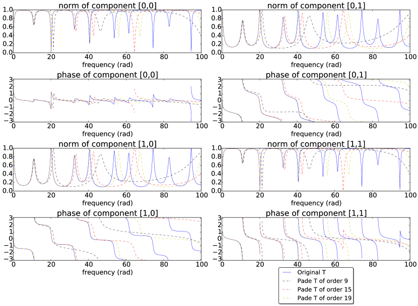
Figure 14: The approximated transfer functions resulting from applying the Padé approximation on individual delays in the network. Although we see that this approximation converges, the peaks often do not occur at the correct locations, as opposed to the approximations resulting from the zero-pole interpolation (compare to Figure 8).

We see in Figure 14 that the peaks in the approximating functions often do not occur in same locations as the peaks of the original transfer function. This may be problematic when attempting to simulate many physical systems for which the locations of the peaks correspond to particular resonant frequencies that have physical relevance. For instance, if one chooses to introduce other components to the system, such as atoms, the resonant frequencies due to the trapped modes of the network must be described accurately or else the resulting dynamics of the approximating system may not correspond to the true dynamics of the physical system. For this reason, using the Padé approximation may not always be the best choice.

Appendix E Blaschke-Potapov Product in the limit ${\Re(z)\to-\infty}$

In Section 8, we proposed a criterion for checking when the multiplicative integral component in Section 5.1 was not necessary. We assumed that the Blaschke-Potapov product converged to a nonzero constant in the limit ${\Re(z)\to-\infty}$. In this section, for demonstrative purposes we show this is the case for the example of a single trapped cavity discussed in Section 4.

In order to examine the convergence of the product in Eq. (14) of Section 4, we write it in the following way. We observe by taking the logarithm with an appropriate branch cut that

$$\prod_{n}\bigl{(}1+a_{n}(z)\bigr{)}$$ (54)

converges if and only if the infinite sum

$$\sum_{n}a_{n}(z)$$ (55)

converges, assuming $\sum_{n}|a_{n}(z)|^{2}$ converges. We take

$$a_{n}(z)=1-\frac{z+p_{n}}{z-\overline{p_{n}}}=\frac{2\Re(p_{n})}{z-p_{n}}.$$ (56)

Using the relation

$$\cot(z)=\sum_{n\in\mathbb{Z}}\frac{1}{z-n\pi},$$ (57)

we get that

$$\lim_{\Re(z)\to-\infty}\sum_{n}a_{n}(z)=-\ln(r).$$ (58)

Actually, higher-order terms of the logarithm expansion of Eq. (54) go to zero in this limit, so we get that

$$\lim_{\Re(z)\to-\infty}\tilde{T}(z)=\lim_{\Re(z)\to-\infty}-\prod_{n\in\mathbb{Z}}\biggl{(}\frac{z+\overline{p_{n}}}{z-p_{n}}\biggr{)}=\lim_{\Re(z)\to-\infty}-\prod_{n}\bigl{(}1+a_{n}(z)\bigr{)}=-1/r.$$ (59)

This shows the desired result that the infinite product in this limit goes to a nonzero constant. Also interestingly, we have been able to compute this value and remark that it is indeed equal to $\lim_{\Re(z)\to-\infty}T(z)$.

The above example with a single trapped cavity formed is illustrative of typical behavior for more complicated systems formed by networks of beamsplitters and time delays. The zero-pole pairs of the system occur in a region of bounded positive real part, and roughly uniformly along the imaginary axis. This suggests that the Blaschke-Potapov product resulting from the zero-pole interpolation will converge to a nonzero constant in the ${\Re(z)\to-\infty}$ limit under quite general circumstances.

References

- [1] Joseph A. Ball, Israel Gohberg, and Leiba Rodman. Tangential interpolation problems for rational matrix functions. Proc. Sympos. Pure Math., 40, 1990.
- [2] L. M. Delves and J. N. Lyness. A numerical method for locating the zeros of an analytic function. Mathematics of Computation 21, 543-560., 1967.
- [3] Bernd Fritzsche, Victor Katsnelson, and Bernd Kirstein. Topics in interpolation theory, volume 95. Birkhäuser, Basel, 2012.
- [4] J. Gough and M. R. James. Quantum feedback networks: Hamiltonian formulation. Communications in Mathematical Physics, 287.3:1109–1132, 2009.
- [5] J. Gough and M. R. James. The series product and its application to quantum feedforward and feedback networks. IEEE Trans. on Automatic Control, 54(11):2530–2544, 2009.
- [6] J. E. Gough, R. Gohm, and M. Yanagisawa. Linear quantum feedback networks. Phys. Rev. A, 78(062104), 2008.
- [7] J. E. Gough, M. R. James, and H. I. Nurdin. Squeezing components in linear quantum feedback networks. Physical Review A, 81.2(023804), 2010.
- [8] Arne L. Grimsmo. Time-delayed quantum feedback control. Phys. Rev. Lett. 115, 060402, 2015.
- [9] Madalin Guta and Naoki Yamamoto. System identification for passive linear quantum systems. arXiv:1303.3771v2, 2014.
- [10] Robin L. Hudson and Kalyanapuram R. Parthasarathy. Quantum ito’s formula and stochastic evolutions. Communications in Mathematical Physics, 93.3:301–323, 1984.
- [11] Peter Kravanja and Marc Van Barel. Computing the zeros of analytic functions. Number 1727. Springer Science & Business Media, 2000.
- [12] James Lam. Model reduction of delay systems using pade approximants. International Journal of Control, 57(2):377–391, 1993. DOI: 10.1080/00207179308934394.
- [13] Aline I. Maalouf and Ian R. Petersen. Coherent control for a class of linear complex quantum systems. Proceedings of the American Control Conference ACC 2009, St. Louis, Missouri, 2009.
- [14] Aline I. Maalouf and Ian R. Petersen. Coherent control for a class of annihilation-operator linear quantum systems. IEEE Transactions on Automatic Control, 56(2):309–319, 2011.
- [15] K. R. Parthasarathy. An introduction to quantum stochastic calculus, volume 85 of Monographs in Mathematics. Birkhauser, Basel, 1992.
- [16] Ian R. Petersen. Quantum linear systems theory. Proceedings of the 19th International Symposium on Mathematical Theory of Networks and Systems, 2010.
- [17] Ian R. Petersen. Analysis of linear quantum optical networks. arXiv preprint arXiv:1403.6214, 2014.
- [18] H. Pichler and P. Zoller. Photonic quantum circuits with time delays: A matrix product state approach. arXiv preprint arXiv:1510.04646, 2015.
- [19] Vladimir Petrovich Potapov. The multiplicative structure of j-contractive matrix functions. Trudy Moskovskogo Matematicheskogo Obshchestva, 4:125–236, 1955.
- [20] J. P. Richard. Time-delay systems: an overview of some recent advances and open problems. Automatica, 39(10):1667–1694, 2003.
- [21] A. J. Shaiju and Ian R. Petersen. A frequency domain condition for the physical realizability of linear quantum systems. Automatic Control, IEEE Transactions on 57.8, pages 2033–2044, 2012.
- [22] Gil Tabak. potapov_interpolation. https://github.com/tabakg/potapov_interpolation.
- [23] Nikolas Tezak, Armand Niederberger, Dmitri S. Pavlichin, Gopal Sarma, and Hideo Mabuchi. Specification of photonic circuits using quantum hardware description language. Philosophical Transactions of the Royal Society of London A: Mathematical, Physical and Engineering Sciences, 370(1979):5270–5290, 2012.
- [24] Masahiro Yanagisawa and Hidenori Kimura. Transfer function approach to quantum control-part i: Dynamics of quantum feedback systems. Automatic Control, IEEE Transactions on, 48.12:2107–2120, 2003.
- [25] G. Zhang and M. R. James. Quantum feedback networks and control: A brief survey. Chinese Science Bulletin, 57(18):2200–2214, 2012.