A unifying framework for understanding state-dependent network dynamics in cortex

Abstract

Activity in neocortex exhibits a range of behaviors, from irregular to temporally precise, and from weakly to strongly correlated. So far there has been no single theoretical framework that could explain all these behaviors, leaving open the possibility that they are a signature of radically different mechanisms. Here, we suggest that this is not the case. Instead, we show that a single theory can account for a broad spectrum of experimental observations, including specifics such as the fine temporal details of subthreshold cross-correlations. For the model underlying our theory, we need only assume a small number of well-established properties common to all local cortical networks. When these assumptions are combined with realistically structured input, they produce exactly the repertoire of behaviors that is observed experimentally, and lead to a number of testable predictions.

Given the immense complexity and computational power of the mammalian cortex, it is perhaps surprising that under a broad range of conditions neurons are relatively stereotyped: spikes are irregular – often near Poisson[1, 2] – and weakly correlated[3, 4], and membrane potentials exhibit approximately Gaussian variability [5, 6]. This apparent randomness was explained by van Vreeswijk and Sompolinsky, who showed that high variability is a necessary consequence of the high yet sparse connectivity, strong synaptic coupling, and relatively low firing rates that are ubiquitous in cortex[7, 8]. This was an important advancement, as understanding the bulk of neuronal activity is a prerequisite for understanding how networks carry out computations, and van Vreeswijk and Sompolinsky’s theory has developed into the de-facto standard model of cortical dynamics.

Although this standard model generally provides a good description of the behavior of neurons, there are a growing number of observations, most of them based on intracellular recordings in vivo, that are at odds with it: near-synchronous activity [9, 10, 11], precise relative timing between excitation and inhibition[12, 13, 11, 14, 15], non-Gaussian membrane potential variability[16, 11], and rapid switching between states that is mediated by both behavior[10] and sensory stimuli[17]. These observations would seem to suggest that the standard model needs to be extended, if not replaced altogether. Here we show that it does, indeed, need to be extended, but in a way that does not require additional anatomical or physiological assumptions. The standard model describes behavior in a regime in which networks exhibit a stable equilibrium at moderate firing rates. Our proposal is to also allow networks to operate in a regime in which the stable equilibrium shifts to zero or near zero firing rates. This extended standard model, like the standard one, is a model of randomly connected networks of excitatory and inhibitory neurons. We investigate analytically, and through simulations, the dynamics of these networks, and what we find is that even unstructured, randomly connected networks can exhibit the behavior reported in a wide variety of studies [18, 9, 19, 12, 5, 20, 16, 13, 21, 22, 11, 10, 15, 14, 23, 24, 25, 17, 3, 4, 26, 27, 6, 28, 29, 30]. This does not imply that networks in the brain are randomly connected. It does, though, imply that to uncover the computational principles used by the brain, it will be necessary to design experiments that go beyond the dynamics expected from randomly connected excitatory-inhibitory networks.

RESULTS

We study the dynamics of a model for a generic local cortical network with a radius of up to about 150 microns and containing on the order of thousands of recurrently connected excitatory and inhibitory neurons. One may think of this network as representing a layer within a cortical column. We assume only a small set of well-established properties: every neuron receives hundreds to thousands of inputs from within its local neighborhood; synaptic coupling is strong (strong enough that without inhibition the network would be epileptic[31]), with an average EPSP size of approximately 0.5 mV[32]; neurons are sparsely connected; and, because inhibition is primarily local within cortex[33], external input to the local network from the “rest of the brain” is assumed to be excitatory. Given these properties, we determine the range of possible behaviors of the network. To do that, we write down a relatively generic network model, argue that the behavior of the network is determined largely by the conductances, and then study their behavior. In the next two sections we present the mathematical formulation of our model and our approach to elucidating its dynamics; in the three sections after that we present the results.

Network model

We consider a network of $N_{E}$ excitatory and $N_{I}$ inhibitory neurons coupled via spike-driven conductance changes and exhibiting essentially arbitrary single neuron dynamics. The network is described by a set of equations for the membrane potentials. Using $V_{i}^{\alpha}$ to denote the membrane potential of neuron $i$ of type $\alpha$, where $\alpha$ can be either $E$ (excitatory) or $I$ (inhibitory), the equations are

$$C_{m}\frac{dV_{i}^{\alpha}}{dt}=I_{i}^{\alpha}(V_{i}^{\alpha},{\bf c}_{i}^{\alpha})-G_{i}^{\alpha E}\big{(}V_{i}^{\alpha}-\mathcal{E}_{E}\big{)}-G_{i}^{\alpha I}\big{(}V_{i}^{\alpha}-\mathcal{E}_{I}\big{)}+I_{i}^{\alpha,ext}(t)\,.$$ (1)

Here $C_{m}$ is membrane capacitance, $I_{i}^{\alpha}(V_{i}^{\alpha},{\bf c}_{i}^{\alpha})$ specifies the single neuron dynamics (including spike generation), ${\bf c}_{i}^{\alpha}$ is a set of channels for neuron $i$, each with its own dynamics, $I_{i}^{\alpha,ext}(t)$ is external, $\mathcal{E}_{E}$ and $\mathcal{E}_{I}$ are reversal potentials, and $G_{i}^{\alpha E}$ and $G_{i}^{\alpha I}$ are the total excitatory and inhibitory conductances,

$$G_{i}^{\alpha\beta}(t)=\sum_{j=1}^{N_{\beta}}W_{ij}^{\alpha\beta}g_{j}^{\beta}(t)$$ (2)

where $W_{ij}^{\alpha\beta}$ are synaptic strengths and the $g_{j}^{\beta}(t)$ are the individual conductance – essentially, $g_{j}^{\beta}(t)$ exhibits a small increase whenever neuron $j$ of type $\beta$ fires. Note that both $I_{i}^{\alpha}$ and the conductance changes can be chosen from a variety of standard models, making Eq. (1) extremely general – it can display single neuron dynamics ranging from linear integrate and fire to Hodgkin-Huxley, and the conductance changes can range from simple functions of time (e.g., instantaneous rise and exponential decay) to complex dynamics that includes failures and adaptation. For our simulations, $I_{i}^{\alpha}$ corresponds to a quadratic integrate and fire neuron and the conductance changes exhibit an instantaneous rise whenever there’s a spike, followed by an exponential decay; see Methods for details, including network parameters.

To analyze the dynamics of the network described in Eq. (1), we focus on the conductances, $G_{i}^{\alpha\beta}(t)$, associated with the recurrently generated spikes. That’s because if we knew the conductances, we would know the activity of the neurons. Importantly, that activity is approximately independent of the single neuron model we use, since for essentially all single neuron models the effect of the conductances is the same: increasing the excitatory conductance increases firing rates, increasing the inhibitory conductance decreases firing rates, and increasing the fluctuations of either of them increases irregularity. Thus, our results apply to other single neuron models besides the quadratic integrate and fire.

Our starting point for analyzing the conductances is similar to that of other mean field models of neuronal networks, [34, 8, 35, 36, 37, 38, 39, 4] which is to divide the conductance seen by each neuron into mean and fluctuating pieces,

$$G_{i}^{\alpha\beta}(t)=G_{\alpha\beta}(t)+\delta G_{i}^{\alpha\beta}(t)$$ (3)

where $G_{\alpha\beta}(t)$ is the population-averaged conductance (the “shared” term) and the $\delta G_{i}^{\alpha\beta}(t)$ are the neuron-specific offsets from – and fluctuations around – that average (the “individual” term); see Figs. 1a and b. The vast majority of mean field models consider what is known as the asynchronous regime, a regime in which the shared conductances, the $G_{\alpha\beta}$, are constant. A key, and nontrivial, result that has come out of those models is that the individual terms, the $\delta G_{i}^{\alpha\beta}(t)$, are rapidly fluctuating, and the fluctuations are weakly correlated across neurons [7, 34, 8, 35, 36, 37, 38, 39, 4]; exactly what is seen in Fig. 1c.

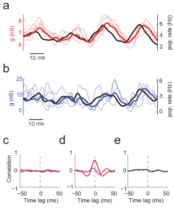
Figure 1: The properties of the individual and shared conductances are consistent with theoretical predictions. a. Excitatory-to-excitatory conductances, $G_{i}^{EE}(t)$, onto five neurons (thin red lines), the shared excitatory-to-excitatory conductance, $G_{EE}(t)$ (thick red line), approximated by averaging over $20$ neurons, and the excitatory population firing rate, $\nu_{E}(t)$ (black line). As predicted, the individual conductances, $\delta G_{i}^{EE}(t)=G_{i}^{EE}(t)-G_{EE}(t)$, show fast and strong fluctuations around the shared conductance, and the shared conductance is proportional to the excitatory population firing rate. b. Analogous to panel a but for inhibitory-to-excitatory conductances, $G_{i}^{EI}(t)$, onto the same five neurons (thin blue lines), the shared inhibitory-to-excitatory conductance, $G_{EI}(t)$ (thick blue line), and the inhibitory population firing rate, $\nu_{I}(t)$ (black line). c. Cross correlations between individual conductances, $\delta G_{i}^{\alpha\beta}(t)$, onto two randomly chosen neurons. Red: cross correlation between two excitatory-to-excitatory individual conductances; purple: cross correlation between excitatory-to-excitatory and inhibitory-to-excitatory individual conductances (onto the same two neurons). In agreement with the theory, the individual conductances are essentially uncorrelated. ḍ. Same as panel c, but for the total (shared plus individual) conductances, $G_{i}^{\alpha\beta}(t)$. The absence of correlations in the individual conductances (panel c) implies that the high correlations in the total conductances (this panel) are entirely due to the correlations in the shared conductances, which in turn are due to the fluctuations in the population rates (panels a and b). e. Cross correlation of the membrane potential between the same two neurons as in panels c and d. Because inhibition largely cancels excitation, the membrane potentials are almost completely uncorrelated. Network parameters are described in Methods.

What we do that is new is extend these results to the case of time-varying shared conductances (the $G_{\alpha\beta}$ depend on time). This time dependence introduces strong correlations in the input to single neurons (as shown, for example, in Fig. 1d), and so leads to qualitatively different behavior compared to the asynchronous regime. To understand this behavior, we need a model for how the shared conductances depend on time. For that we make use of two observations. First, as we show in Methods, and as can be seen in Figs. 1a and b, the shared conductances are proportional to the average excitatory and inhibitory firing rates, with the constant of proportionality given by the connection strengths,

$$G_{\alpha\beta}(t)\propto W_{\alpha\beta}\nu_{\beta}(t)$$ (4)

where $W_{\alpha\beta}$ is the average synaptic strength made by a neuron of type $\beta$ onto a neuron of type $\alpha$, assuming that a connection is made, and $\nu_{\beta}(t)\equiv N_{\beta}^{-1}\sum_{j}\nu_{j}^{\beta}(t)$ is the average firing rate of population $\beta$.

Second, we use a highly successful phenomenological model of the average firing rates, the Wilson and Cowan model[40],

$$\tau_{E}\frac{d\nu_{E}}{dt} =f_{E}\big{(}J_{EE}\nu_{E}-J_{EI}\nu_{I}+I_{E}(t)\big{)}-\nu_{E}$$ (5a)

$$\tau_{I}\frac{d\nu_{I}}{dt} =f_{I}\big{(}J_{IE}\nu_{E}-J_{II}\nu_{I}+I_{I}(t)\big{)}-\nu_{I}$$ (5b)

where $f_{E}$ and $f_{I}$ are approximately sigmoidal gain functions, $J_{\alpha\beta}$ is approximately proportional to $W_{\alpha\beta}$, and $I_{E}(t)$ and $I_{I}(t)$ represent external input. While this model can’t provide quantitative results, it can place severe constraints on the firing rate dynamics, and thus on the dynamics of the shared conductances. Consequently, it allows us to categorize the expected range of network behaviors, and thus, via Eq. (3) and Eq. (4), predict single-neuron sub-threshold dynamics, including properties of correlations across neurons.

Two distinct network states

To understand the constraints implied by the Wilson and Cowan model, and, therefore, the possible range of network behaviors, we apply phase plane analysis. This analysis starts by constructing the excitatory and inhibitory nullclines, which are curves in $\nu_{E}$-$\nu_{I}$ space along which $d\nu_{E}/dt$ and $d\nu_{I}/dt$ are zero, respectively. Then, given the nullclines, network dynamics can be inferred relatively easily (see Fig. 2 caption). For essentially any reasonable shape of the gain functions, $f_{E}$ and $f_{I}$, two qualitatively different regimes can be identified [41]. One corresponds to the “active state,” for which the nullclines intersect at nonzero rate (Fig. 2a, b); the other to the “quiescent state,” for which the nullclines intersect at near zero rate (Fig. 2c).

Network models typically consider only the active state [7, 8, 34, 2, 35, 36, 37, 38, 39, 4]. However, the quiescent state is just as important. In fact, as we will show, it is key to explaining, and reconciling, a diverse set of in vivo cortical data. In the next three sections we elaborate on this point, using as a guide the nullclines given in Fig. 2. We first briefly review – and extend – the properties of the active state (Figs. 2a and b); we then describe the properties of the quiescent state (Fig. 2c); and, finally, we discuss switches between the two.

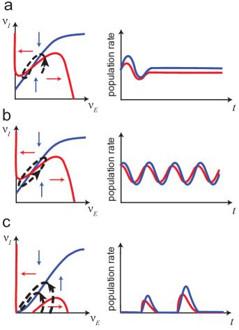
Figure 2: Nullclines and population-averaged firing rates, or “population rates”, corresponding to Eq. (5), in three different regimes. Left panels: excitatory (red) and inhibitory (blue) nullclines. Points along the excitatory nullcline represent firing rate equilibria at fixed inhibition; above it the excitatory firing rate decreases with time while below it the excitatory firing rate increases (red arrows). Correspondingly, points along the inhibitory nullcline represent firing rate equilibria at fixed excitation; to the left of it the inhibitory firing rate decreases while to the right of it the inhibitory firing rate increases (blue arrows). The dashed black curves correspond to trajectories. Right panels: population rates; red lines are excitatory population rates and blue ones are inhibitory rates. See reference 41 for a detailed description of how these nullclines are constructed. a. The input is sufficiently strong that there is a robust, low population rate equilibrium, and inhibition is sufficiently fast that the equilibrium is stable[8, 41]. The trajectory that spirals into the fixed point represents transient behavior; after long times the population rates are constant, as shown in the right panel. b. Same as panel a, but with slower inhibition, which destabilizes the equilibrium. In this regime the population rates oscillate. c. Sufficiently weak input that the only equilibrium is at near zero population rate. The network is still excitable, though, and brief, strong input produces transient activity, as shown by the two trajectories in the right panel.

The active state

The active state is characterized by an equilibrium at nonzero population rates. This equilibrium, however, may or may not be stable. Let us first consider the stable case, for which the network exhibits constant mean excitatory and inhibitory population rates, as shown in Fig. 2a. Because the shared conductances, the $G_{\alpha\beta}$, are proportional to the population rates (see Eq. (4)), they too are constant, and so the dynamics of single neurons are determined solely by the individual conductances, the $\delta G_{i}^{\alpha\beta}$. As has been shown previously (and as we show in Figs. 1a and b), these conductances exhibit essentially stochastic, uncorrelated fluctuations [7, 8, 38, 39]. This leads to approximately Gaussian distributed conductances, and, consequently, approximately Gaussian distributed membrane potentials. Dynamic balance [7, 8] ensures that the mean excitatory and inhibitory currents nearly cancel each other, so that spiking is caused by the stochastic fluctuations of the membrane potentials. This results in irregular spike times that are very weakly correlated across neurons [4]. Strongly-coupled spiking networks operating at a stable equilibrium have become the de-facto standard model of cortical network dynamics [7, 8, 34, 35, 41, 36, 38, 39, 4], and the dynamic properties in this regime are referred to as the “asynchronous state”.

Although a constant population rate equilibrium is a convenient abstraction, in fact population rates are never constant. That’s because finite-size effects produce fluctuations, which in turn lead to trajectories that spiral in a counter-clockwise direction around the equilibrium. The resulting time-depending population rates produce, via Eq. (4), time-dependent fluctuations in the shared conductances, and thus strong correlations. This would seem to rule out operation in the asynchronous regime, which by definition is characterized by essentially uncorrelated membrane potentials and action potentials. However, because of the nearly tangential intersection of the excitatory and inhibitory nullclines, the trajectories are elongated (Fig. 2b), and so the shared excitatory and inhibitory conductances closely track each other. This close tracking causes the correlations to mostly cancel, producing nearly uncorrelated membrane potentials, and, consequently, irregular spike times that are also nearly uncorrelated. These predictions, which are consistent with rigorous analytic results for networks of binary neurons [4], are illustrated in Fig. 1 (see in particular panel e, which shows a complete absence of correlations in the membrane potential). Thus, even though the excitatory and inhibitory conductances are strongly correlated across neurons, their difference (suitably weighted by the reversal potentials) is not, and so even finite size networks can exhibit asynchronous activity. This can be seen in our network simulations (Fig. 3a and b), in vivo recordings (Fig. 3c and d), and numerous other simulation studies [8, 34, 35, 41, 36, 37, 38, 39, 4].

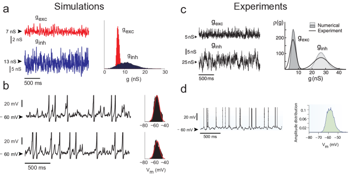
Figure 3: Simulations and in vivo data in the active state. a. Conductance traces and histograms from simulations. Conductances are approximately Gaussian distributed, and inhibitory conductances have a larger mean and wider distribution than excitatory ones. Network parameters,which are described in Methods are the same as for Fig. 1. b. Membrane potential traces and histograms from the same set of simulations as in panel a. Sub-threshold membrane potentials are approximately Gaussian distributed, and spike timing is irregular and asynchronous across neurons. c. Conductance traces and histogram in vivo, adapted from Fig. 7b of reference 6; permission requested. d. Membrane potential traces and histograms in vivo, adapted from Box 1a of reference 5, with permission from Macmillan Publishers Ltd: Nat. Rev. Neurosci., copyright 2003.

The active state also applies when the population rates change slowly. These slow changes can occur either because the external input is time varying, or because the population rate equilibrium becomes unstable, producing oscillations [40, 8, 41, 37]. In either case the population rates become correlated and, therefore, so do the excitatory and inhibitory conductances (see Eq. (4)). However, as in the case of fluctuations driven by finite size effects, the shared excitatory and inhibitory conductances again nearly cancel. Thus, almost all of the results for constant input apply to time-varying input and oscillations: excitatory and inhibitory conductances inherit cross-correlations from the time-varying population rates, but the cancellation of these correlations at the level of the membrane potentials, in combination with the strongly fluctuating conductance terms, lead to irregular spiking and approximately Gaussian-distributed membrane potentials. Moreover, conditioned on population rates, both the membrane potential and spike times are approximately uncorrelated, and the network remains effectively asynchronous.

How slowly do the changes in population rate need to be for the network to stay asynchronous? It turns out that the external input can change on a faster time scale than that of single-neuron dynamics; this is, in fact, one of the hallmarks of strongly-coupled balanced networks[8]: sudden, strong increases in input can induce a sudden rise in excitation before inhibition can catch up, causing many neurons to spike almost simultaneously. When this happens, neurons can display increased temporal precision in spike timing in response to sharp stimulus onsets, which provides a robust, network-level explanation of precise timing effects in cortex [18].

Although the active state has provided a great deal of insight into cortical dynamics, there is a growing body of experimental data that is not consistent with it. As we will show in the next two sections, the other nullcline regime – the one corresponding to the quiescent state – is needed to provide a robust explanation of that data.

The quiescent state

In the active state, the external input is strong enough for the network to stay continuously active. What happens if we reduce its strength? This will cause the excitatory nullcline to shift down and the inhibitory nullcline to shift to the right. For small enough external input – and thus large enough shifts – the equilibrium vanishes. When this happens, a new, stable equilibrium appears at zero or near zero population rate (Fig.2c, which shows an equilibrium at zero firing rate). This equilibrium corresponds to a silent or nearly silent network, which is why we refer to the corresponding nullcline regime as the quiescent state.

While a silent network may seem uninteresting, the strong recurrent connections among the excitatory neurons means that such a network is highly excitable. Consequently, excitatory input can result in nontrivial dynamics. Two typical population rate trajectories caused by brief input applied to a silent network are shown in Fig. 2c, both in phase space (left panel) and versus time (right panel). Note that the trajectories are highly stereotyped: they all consist of a sudden, rapid increase in excitatory population rate, followed, with a small delay, by a rapid increase in inhibitory rate, and then a slightly slower – but still fast – drop in both excitatory and inhibitory population rates. Thus, sufficiently strong input applied to the quiescent state results in short bursts of activity in which inhibition peaks slightly later than excitation. These bursts differ in amplitude, but vary little in shape.

Because population firing rates are related to conductances (Eq. (4)) and conductances drive neurons (Eq. (1)), knowing how the population firing rates evolve over time allows us to make inferences about the behavior of individual neurons. Consequently, Fig. 2c leads to the following picture: between bursts of activity the synaptic drive is essentially zero and the neurons are at rest; during a burst, first the shared excitatory conductance to each neuron increases very rapidly, and then, a few milliseconds later, the shared inhibitory conductance increases very rapidly; after they have peaked, they decay back toward zero, with both decaying at about the same rate.

To verify this picture, we analyzed the same network as in our previous simulations (Fig. 3), but with input that consisted of brief pulses rather than sustained drive. As predicted, the conductances in the simulations showed large, brief excursions which were highly correlated across neurons, excitation led inhibition by a small amount, and there was on average no time lag between the excitatory drives on pairs of neurons or between the inhibitory drives (Fig. 4a).

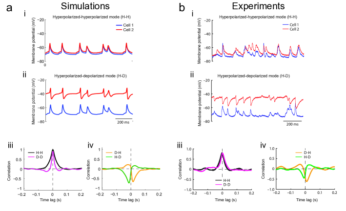
Figure 4: Simulations and in vivo data during brief excursions from the quiescent state. a. Simulations. The excursions were caused by brief, synchronous input applied to the whole network. Data is shown for two neurons; for these neurons the single neuron dynamics was linearized to prevent spiking, and constant current was injected to adjust the resting membrane potential (see Methods). In panel a-i the resting membrane potential was set to -70 mV (the inhibitory reversal potential) to isolate the excitatory drive. (Cell 2 was offset slightly to aid visibility.) In panel a-ii the resting membrane potential was set to -40 mV to (partially) isolate the inhibitory drive. Because isolation was incomplete, there are brief upward deflections associated with the initial surge of excitation. Panel a-iii shows the membrane potential correlation between cells 1 and 2 when they are both hyperpolarized to -70 mV (H-H; black) and when they are both depolarized to -40 mV (D-D; magenta). Panel a-iv shows the same thing, but when cell 1 is depolarized and cell 2 is hyperpolarized (D-H, orange trace) and when cell 1 is hyperpolarized and cell 2 is depolarized (H-D, green trace). Because of our convention for computing the correlation (see Methods), the minimum at a positive lag for the orange trace and a negative lag for the green trace both indicate that excitation leads inhibition. Network parameters, which are described in Methods, are the same as for Figs. 1 and 3 except for the input. b. Same as panel a, except for experimental data. Reproduced with permission from reference 11.

In vivo experiments have, critically, verified that the quiescent state exists in cortex, and that excitation of the quiescent state leads to behavior consistent with our predictions. In particular, DeWeese and Zador observed brief membrane potential excursions (which the authors called “bumps”) separated by periods of silence, and they established that during the silent periods there was essentially no synaptic drive[16].

More detailed experiments involving paired recordings from nearby neurons in somatosensory cortex of anesthetized rats [11] yielded results that are identical to our predictions of the relative timing of excitation and inhibition across pairs of neurons. In those experiments, excitatory and inhibitory drive to different neurons occurred at about the same time, whereas excitation led inhibition by several milliseconds, on average. A time lag between excitation and inhibition was also seen in single neuron intracellular recordings in anesthetized rat auditory cortex[12]. Although in the latter study the authors could not directly compute cross-correlograms, they could compute trial-averages of both excitatory and inhibitory drive, and they reported that “inhibition and excitation occurred in a precise and stereotyped temporal sequence,” with excitation leading inhibition by a few milliseconds, again in agreement with our predictions.

The absence of a time lag for both excitation and inhibition across different neurons, and the short lag of inhibition behind excitation during these brief events, is exactly what our theory predicts – both qualitatively and quantitatively (see Figs. 4a and b). However, although in some experiments cortical networks spend much of their time in the quiescent state, with only brief periods of activity, more commonly they switch – often fairly rapidly – between the quiescent and active states. We consider that behavior next.

State switching

In the quiescent state, brief supra-threshold input produces short, stereotyped bursts of activity. Longer supra-threshold input leads to different dynamics: instead of exhibiting brief stereotyped activity bursts, the network switches to the active state; that is, the nullclines switch to the topology shown in Fig. 2a[41]. The transition from the quiescent to the active state has the same properties as the initial phase of the brief activity bursts: it occurs synchronously in all neurons, and the spikes at the onset are closely temporally aligned (in contrast to later spikes). When the input falls below threshold, the network becomes quiescent again; this also occurs synchronously on all neurons, although with somewhat less precision than for the quiescent-to-active transition. Repeated alternations between super-threshold and sub-threshold input is what we call state switching (see Fig. 5).

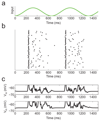
Figure 5: Spike rasters and membrane potential during state switching. a. The input to the network consists of a slowly oscillating sinusoid. b. Spike rasters. As predicted, spikes are highly synchronous during the transition from the quiescent to active state, but quickly desynchronize. c. Membrane potential of two randomly chosen neurons. In the active state, fluctuations are large and, especially at the initial onset, highly correlated. In the quiescent state, on the other hand, the membrane potential is virtually flat. Network parameters, which are described in Methods, are the same as for Figs. 1, 3 and 4 except for the input.

Note that state switching is very different from the bursts of activity that occur when the quiescent state is activated by brief input. For state switching, the nullcline topology alternates between that shown in Figs. 2a and b and that shown in Fig. 2c (discussed in detail in reference 41). Therefore, termination of the active state occurs either through a decrease in external input or a change in single neuron properties (e.g., spike after-hyperpolarization, as discussed in the next paragraph). For brief bursts of activity, on the other hand, the nullclines do not change, and activity is terminated by inhibition.

Although state switching can be driven by external input, it can also occur spontaneously, without changes in external input. This is because modulation in single-neuron excitability has the same effect as changing the strength of the external input. A typical example of such a modulation is spike after-hyperpolarization, which results in a slow decrease in the effective strength of the input during active periods and a slow increase during quiescent periods. Therefore, even with constant external input, there can be shifts in the nullclines that produce sudden switches between active and quiescent state dynamics. The resulting activity is commonly referred to as up and down states. Such a mechanism, which was first described in the context of networks for generating breathing [42], has been confirmed both theoretically [41, 43, 44] and experimentally [45, 46].

Internally driven up-down states are not the only example of state switching. In fact, a central prediction of our theory is that any local cortical network will undergo state switching whenever the effective input switches between sustained supra-threshold and sub-threshold levels. In the supra-threshold regime, the network will have all of the properties of the active state, including weak correlations in membrane potential and spike times (at least after the initial transient). However, correlations computed in periods that are long compared to the switching time will be stronger – typically much stronger. That’s because the switches occur in all neurons nearly synchronously. Consequently, the membrane potential on any one neuron is highly predictive of the membrane potential on any other neuron (i.e., high membrane potential on any one neuron predicts high membrane potential on another, and similarly for low membrane potential.)

To illustrate the effect of state switching on correlations across neurons, we performed simulations using the same randomly connected spiking network as for our previous results (Figs 2 and 3). Unlike in the previous simulations, however, we switched between two input regimes: (1) a regime in which the input consisted of slow oscillations that periodically crossed the network-activating threshold, termed “Sub/Suprathreshold”, and (2) a regime in which the input had a rich temporal structure, and which kept the network continuously active, termed “Suprathreshold”. The choice of the two input regimes and their structure were motivated by experiments[10], as detailed below.

When we stimulated our network with the Sub/Suprathreshold input, whenever the input crossed the threshold from below, a transition from the quiescent to the active state occurred; when it crossed from above, the opposite transition occurred. As predicted by our theory, in this regime membrane potentials were highly correlated, as shown in the Sub/Suprathreshold regions of Fig. 6a. (Note that the only important feature of the input in this regime is the repeated crossing of the activation threshold; the crossings do need not to be caused by oscillating input, nor do need they need to be at regular intervals.)

In the Suprathreshold regime, the input consisted of repeated temporal Gabor filters with a center frequency of 8 Hz; this was meant to mimic whisking-like input (compare to Fig. 1i in reference 10). In this regime, despite the strong and fast modulation of input amplitude, the input was sustained enough to keep the network in the active state, yet it was weak enough that the time-average of single-neuron firing was $\leq 1$ Hz; about the same firing rate as during the Sub/Suprathreshold input. Because in the Suprathreshold regime the network is in the active state, our prediction is that membrane potential correlations should be low, despite strong fluctuations in the input. Indeed they are, as can be seen in the central region in Fig. 6a.

Exactly such behavior was found in a recent study by Poulet and Petersen [10] who, in an experimental tour de force, recorded membrane potentials in awake animals in pairs of neurons in mouse somatosensory cortex. Their finding was that the degree of membrane potential correlations was tightly linked to the behavioral state of the animal: during quiet resting, membrane potentials of nearby neurons were highly correlated, whereas during active whisking, correlations decreased markedly (Fig. 6b). Within our framework, this is expected if the input to the sensory cortex alternates between supra-threshold and sub-threshold during quiet resting, but is sustained during active whisking. As for the origin of the intermittent input during quiet resting, our theory suggests a number of possibilities: it could be due to invading activity from other cortical or subcortical areas, an operating regime that is close to the activation threshold together with adaptation effects (analogous to spontaneous up-down state switching, as described above), or a combination of the two.

A key observation in the experiments by Poulet and Petersen[10] was that even after cutting the sensory nerves that relay whisker sensation to somatosensory cortex, the neurons still switched between high and low correlations whenever the behavior changed between resting and whisking. Based on this observation, our theory predicts that the rodent somatosensory cortex receives sustained input from non-sensory areas whenever the animal is actively whisking.

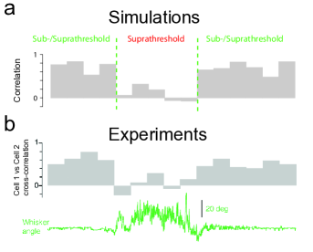
Figure 6: Simulations and in vivo data during state switching. a. Simulations. In the region marked “Sub/Suprathreshold,” the input is identical to that of Fig. 5: slowly oscillating, with amplitude and offset chosen so that near the peaks of the oscillations the network is in the active state and the rest of the time it is in the quiescent state. In the region marked “Suprathreshold,” on the other hand, the input is sufficiently large that the network is always in the active state. In both regions the correlation coefficient of the membrane potentials in two cells is computed over 1 second windows and averaged over the central 4 ms. Network parameters, which are described in Methods, are the same as for Figs. 1 and 3-5 except for the input. b. Same as panel a, except for experimental data (Supplementary Fig. 4 from reference 10). The green trace is whisker angle. According to our theory, the absence of whisking (low angular deflection) corresponds to input that frequently drops below the activation threshold, while whisking (high angular deflection) corresponds to input that stays continuously above the activation threshold. This is reflected in the high correlations in the absence of whisking and the weak correlations during whisking. Reproduced with permission by the author.

DISCUSSION

We have shown how the rich repertoire of cortical networks – ranging from weakly correlated with irregular firing to highly correlated and temporally precise, and including rapid switches between different states – can be readily understood within a single theoretical framework. The mechanistic model underlying this framework is extremely general and its essential ingredients apply to any local patch of cortex.

Our primary result is that cortical networks can operate in one of two distinct regimes, which we termed active and quiescent. In the active regime, the network exhibits ongoing activity with population firing rates that never drop to zero, so that the membrane potentials of all neurons are depolarized away from their resting values. This regime contains as a special case asynchronous activity, in which spiking is irregular, membrane potential distributions are Gaussian, and correlations are weak, as has been studied previously [7, 34, 8, 2, 41, 35, 5, 37, 38, 6, 39, 23, 3, 4]. It also contains oscillating activity[35, 41, 36, 37, 15], and, more generally, activity that fluctuates due to finite-size effects[34], or changes in magnitude due to changes in input strength. In the quiescent regime, on the other hand, the topology of the nullclines is different from that in the active state, and the network is silent or nearly silent. It is, though, highly excitable and brief input results in precisely-timed stereotyped dynamics both at the level of population activity and single-neuron subthreshold activity.

A key result of this work is that the regime in which the network operates is determined primarily by the strength of the external input: sufficiently strong external input leads to the active state; sufficiently weak input to the quiescent state. Importantly, while changes in single-neuron properties can move cortical networks from one state to another, [41, 45] no such changes are required – changing the strength and duration of external spiking input is sufficient.

In which of the two regimes do cortical networks operate in vivo? It appears that the answer is both [1, 2, 18, 9, 45, 5, 12, 19, 20, 6, 21, 22, 13, 16, 10, 11, 30, 15, 14, 23, 24, 26, 3, 4]. However, a consistent observation is that cortical networks do not remain completely silent for any extended period of time. Consequently, networks that do operate in the quiescent state tend to undergo frequent brief activations even in the absence of any sensory stimulation.

Based on the above picture, we make a number of specific predictions, and violation of any of them would invalidate our theory. First, brief activations in the quiescent state are a network effect shaped by the recurrent interactions, so changes in excitatory and inhibitory drive occur in all local neurons nearly simultaneously. To test this prediction, one needs to record intracellularly from at least two nearby neurons. The only study we are aware of that has performed such measurements across many pairs of neurons was carried out in rodent somatosensory cortex[11], and, in line with our theory, excitation and inhibition were synchronous across neurons. We predict that this must be true for any cortical network that operates in the quiescent state, including auditory cortex, for which brief activations of single neurons have been reported previously[12, 19, 16]. Furthermore, our theory predicts that switches between the quiescent and the active state (not just brief, graded excursions) have to occur in all local neurons nearly synchronously, which implies that membrane potentials have to be highly correlated across neurons whenever switches between up and down states are observed in any individual neuron[9]. In essence, observing a single neuron is sufficient to predict the timing and general features of the subthreshold activities of all other nearby neurons.

Second, we predict that the excitatory and inhibitory drives to individual neurons should rise and fall together, with a short lag of inhibition behind excitation – irrespective of network state. This should be true across neurons as well, so for any pair of neurons in a local network, the cross-correlation between excitatory drives and between inhibitory drives should always peak at zero time lag, and the cross-correlation between excitatory and inhibitory drives should exhibit a small time lag. This should be a robust phenomenon that doesn’t depend on either the wiring details nor on the momentary amount of synaptic depression[13].

Third, oscillations should be very common, and should change with network state – a phenomenon that is seen frequently, and often cited as evidence that oscillations are involved in information processing (reviewed in reference 47). Our theory also explains more subtle effects, such as why, during oscillations, bigger excursions in excitation are followed by bigger excursions in inhibition after a short delay of a few milliseconds[15].

Besides making a specific set of predictions, our theory provides an alternative explanation of state switching, which is that it can be caused by simply modulating the strength or temporal features of the external input. Typically, state switching – switching between the active and quiescent states – is attributed to neuromodulators that change the membrane and synaptic properties of neurons[48]. This mechanism is compatible with our framework because, as pointed out above, changes in single neuron properties can, by themselves, cause transitions between the active and quiescent states. However, if all state switches in cortex were to depend on neuromodulation, then both the timing and location of the switches would be difficult to control on either a fine temporal or spatial scale. That’s because neuromodulators are released globally, rather than locally, and the timescale for removing their effect is too long to permit rapid switches.

Neuromodulators are not, of course, the only candidate drivers of state switches. A recent study reported that the level of tonic firing in thalamus can control the state of its target area in cortex[26]. However, the mechanism was speculated to be specific to thalamic input, and separate from the effect of sensory signals transmitted by the thalamus. In contrast, our theory shows that any changes in external input, from any area, can lead to state switching.

Another recent study explored the effect of visual stimuli on the strength and spatial spread of spike-triggered average LFP waves in primary visual cortex (V1)[17]. While such averaged LFP waves were strong without stimulation, they were essentially absent during strong full-field stimulation – in effect, the external input caused a state switch. The authors proposed that this state switch occurred because the external input modified the effectiveness of lateral connectivity, perhaps due to a modulation of the spatial spread of dendritic integration. In light of our theory, however, this phenomenon can be explained by noting that strong sensory input is likely to move the network from a quiescent state punctuated by brief periods of activity to a continually active state. As discussed above, spikes that occur during the brief periods of activity are temporally precise and spatially correlated. Consequently, they exhibit long-range correlations with each other, and thus long-range correlations with the LFP. Spikes that occur during the active state, on the other hand, are irregular and spatially uncorrelated, and thus can exhibit only short range correlations with the LFP.

Implications for information processing

Perhaps the most important conclusion we can draw from our analysis is that observation of any of the phenomena predicted by our theory is not, in and of itself, evidence for any deep computational principle – it is evidence that one is recording from an area with all the properties of a randomly connected network. In particular, one should not be surprised by brief, highly synchronous bursts of activity, [11, 19, 16] precise timing between the excitatory and inhibitory drives to individual or different neurons, [11, 12, 13, 14, 15] oscillations that change with network state[47], or correlations between neurons[10, 25, 26], and between neurons and the local field potential[17] that change with network state.

This does not imply, of course, that the brain doesn’t make use of some – or all – of these phenomena. Indeed, Loebel and colleagues[49] showed theoretically that brief, highly synchronized bursts of activity could provide a precise temporal code for complex sounds; there have been a large number of proposals for the computational role of oscillations[47]; and the ability to control the correlational structure among neurons simply by modifying the input to an area (a key outcome of our model) could play a role in gating information. However, because all of these phenomena occur naturally in randomly connected networks, providing a direct link to an underlying computational principle becomes a nontrivial experimental task.

Conclusions

In sum, starting from a limited set of generic cortical network properties, our theory reconciles and unifies a large body of existing experimental data that previously appeared either unrelated or suggested fundamental differences between cortical areas. At the same time, it makes a set of specific predictions about possible firing patterns and correlational structures for a range of input regimes – predictions that should hold for any layer in any cortical area. To the best of our knowledge, the data in all of the existing studies are in excellent agreement with our theory. However, not all of our predictions have been tested, nor have parameters, layers and areas been thoroughly explored, in large part because of the difficulty of recording intracellularly from multiple cortical neurons in vivo. If our theory does hold up, though, the fact that a relatively simple framework can explain a large variety of electrophysiological recordings in vivo would indicate that, at least at the level of population firing rates and subthreshold and spiking correlations between neurons, cortical network dynamics is reasonably straightforward to understand.

Finally, given that there is a great deal of structure in cortical networks, even at levels that span just several layers within a single column [32], it might seem surprising that a model based on randomly connected networks could explain such a large body of in vivo data. However, it is important to note that the observations we explain are essentially observations about collective properties: excitation and inhibition of individual neurons (which are due to the summation of many presynaptic neurons), membrane potential and single-neuron spike statistics, population-averaged firing rates, correlations, and oscillations. A solid understanding of the universal properties of cortical dynamics, as we have attempted to provide here, is a prerequisite for uncovering those activity patterns that are a signature of specific functional roles.

Acknowledgments

This work was supported by the Gatsby Charitable Foundation and and US National Institute of Mental Health grant R01 MH62447. We would like to thank Ken Harris and David Barrett for insightful comments on the manuscript.

METHODS

The network equations we simulated follow the form of those given in the main text, Eq. (1); all that remains to be specified is the single neuron model, $I_{i}^{\alpha}(V_{i},{\bf c}_{i})$ the equation for the synaptic conductances, the $g_{j}^{\beta}$, and an expression for the external input, $I_{i}^{\alpha,ext}$. For the single neuron model we use a quadratic integrate and fire neuron [50, 41] with parameters that are independent of neuron type, so that $I^{\alpha}(V,{\bf c})\rightarrow I(V)$. Using $R_{m}$ to denote the membrane resistance, $I(V)$ is given by

$$I(V)=\frac{(V-V_{r})(V-V_{th})}{R_{m}(V_{th}-V_{r})}\,.$$ (6)

For the synaptic conductances, $g_{j}^{\beta}(t)$, we assume an instantaneous rise and exponential decay,

$$\tau_{s}\frac{dg_{j}^{\beta}}{dt}=-g_{j}^{\beta}+g_{0}\tau_{s}\sum_{k}\delta\big{(}t-t_{j}^{k}\big{)}\,,$$ (7)

where $g_{0}$ is the conductance associated with a unitary event, $t_{j}^{k}$ is the time of the $k^{\rm th}$ spike on neuron $j$, and $\delta(t)$ is the Dirac delta function. A spike is emitted when the voltage reaches $+\infty$, at which point it is reset to $-\infty$. For the external input we assumed a conductance-based coupling,

$$I_{i}^{\alpha,ext}(t)=W_{\alpha}^{ext}G_{i}^{ext}(t)\big{(}V_{i}^{\alpha}-\mathcal{E}_{E}\big{)}\,.$$ (8)

The conductance associated with the external input, $G_{i}^{ext}(t)$, varied from one simulation to another, and is discussed below.

Connectivity was sparse: the connection probability between any two neurons was 0.1, independent of neuron type. If there was a connection, the normalized connection strengths, $W_{ij}^{\alpha\beta}$, was equal to $W_{\alpha\beta}$ on average, with Gaussian noise around that mean,

$$W_{ij}^{\alpha\beta}=\left\{\begin{array}[]{ll}W_{\alpha\beta}(1+0.1\eta)&\ \ \hbox{probability }0.1\\ 0&\ \ \hbox{probability }0.9\end{array}\right.$$ (9)

where $\eta$ is a zero mean, unit variance Gaussian random variable, taken to be independent across weights.

The network parameters are given in Table I. Note that $R_{m}$ and $C_{m}$ were chosen so that the membrane time constant is 20 ms. The connection strengths, $W_{EE}$, $W_{EI}$, etc., given in that table were chosen to generate the following PSP sizes:

$$\begin{array}[]{ll}E\rightarrow E:\ \ 0.95\hbox{ mV},&\ \ \ \ \ \ E\rightarrow I:\ \ 1.19\hbox{ mV}\\ I\rightarrow E\ :-1.96\hbox{ mV},&\ \ \ \ \ \ \ I\rightarrow I:-1.96\hbox{ mV}\,.\end{array}$$ (10)

To find the connection strengths that generate the right PSP sizes, we linearized the single neuron dynamics around rest ($V_{i}=V_{r})$, computed the PSP amplitude in response to a single presynaptic spike, and adjusted the connection strength to achieve the values given in Eq. (10). The resulting expression for the average weights in terms of PSP amplitudes is [41]

$$W_{\alpha\beta}=\frac{V_{\alpha\beta}}{\mathcal{E}_{\beta}-V_{r}}\frac{1}{R_{m}g_{0}}\frac{\tau_{m}}{\tau_{s}}\exp\left[\frac{\log\tau_{m}/\tau_{s}}{\tau_{m}/\tau_{s}-1}\right]$$ (11)

where $V_{\alpha\beta}$ is the PSP on a neuron of type $\alpha$ given a presynaptic spike on a neuron of type $\beta$. This formula yields the values for the weights given in Table I.

Table I. Network parameters.

number of excitatory neurons, $N_{E}$	1600
number of inhibitory neurons, $N_{I}$	400
connection probability	0.1
membrane resistance, $R_{m}$	100 M$\Omega$
membrane capacitance, $C_{m}$	200 pF
membrane time constant, $R_{m}C_{m}\equiv\tau_{m}$	20 ms
synaptic time constant, $\tau_{s}$	5 ms
unitary conductance, $g_{0}$	0.928 nS
resting membrane potential, $V_{r}$	-65 mV
threshold, $V_{th}$	-50 mV
excitatory reversal potential, $\mathcal{E}_{E}$	0 mV
inhibitory reversal potential, $\mathcal{E}_{I}$	-70 mV
$W_{EE}$	1
$W_{IE}$	1.253
$W_{EI}$	26.82
$W_{II}$	26.82
$W_{E}^{ext}$	1
$W_{I}^{ext}$	0.667

Although we report only simulations with $N=2,000$ neurons, we performed simulations with $N$ ranging from 1,000 to 12,000. For all simulations, the connection probability was fixed at 0.1. The PSP size, however, followed the $K^{-1/2}$ scaling suggested by van Vreeswijk end Sompolinsky [8], where $K$ is the average number of connections per neuron; to achieve this, we scaled the synaptic weights relative to the values shown in Table I by a factor of $(K_{0}/K)^{1/2}$ where $K_{0}=200\,(=\,0.1\times 2,000)$ is the number of connections/neuron when $N=2,000$, and $K=0.1N$. It is also necessary to scale the external connection strengths, but by $K^{1/2}$ instead of $K^{-1/2}$; we thus scaled $W_{E}^{ext}$ and $W_{I}^{ext}$ by a factor of $(K/K_{0})^{1/2}$. With this scaling, results were qualitatively the same for all network sizes.

Simulations were performed using a 4th-order Runge-Kutta integration scheme with a time step of 0.2 ms. To avoid the infinities associated with spike threshold and reset, we made the change of variables $V_{i}=(V_{th}+V_{r})/2+(V_{th}-V_{r})\tan(\theta_{i}/2)$, and integrated $\theta_{i}$ rather than $V_{i}$. This moved the spike threshold and reset to $\theta_{i}=\pi$.

External input

The only difference among the simulations used to make Figs. 1 and 3-6 was the external conductance, $G_{i}^{ext}(t)$. Although ultimately this conductance comes from spikes in other areas, for simplicity we characterized it as a time-dependent function filtered by the synaptic time constant,

$$\tau_{s}\frac{dG_{i}^{ext}}{dt}=-G_{i}^{ext}+g_{0}h_{i}^{ext}(t)\,.$$ (12)

The normalized drive, $h_{i}^{ext}(t)$, was constant for Figs. 1 and 3 (active state), consisted of brief synchronous pulses for Fig. 4 (quiescent state), was sinusoidal for Fig. 5, and alternated between sinusoidal and Gabor functions for Fig. 6 (state switching).

More quantitatively, for Figs. 1 and 3 we used

$$h_{i}^{ext}(t)=5\,.$$ (13)

Because $h_{i}^{ext}(t)$ is constant, for this case $G_{i}^{ext}$ is also constant (and independent of neuron), and equal to $5g_{0}$. Given that the integral of the conductance change per spike is $g_{0}\tau_{s}$ (see Eq. (7)), this corresponds to the mean input produced by 40 neurons firing at rate 25 Hz (40 $\times$ 25 Hz $\times$ 5 ms = 5).

For Fig. 4 the input consisted of 40 ms pulses arriving randomly at an average frequency of 8 Hz, with amplitudes drawn from a uniform distribution. More specifically,

$$h_{i}^{ext}(t)=\sum_{k}a_{k}\hat{T}\big{(}t-(\tau_{k}+\delta t_{i})\big{)}$$ (14)

where $\hat{T}(t)$ is a 40 ms top hat function ($\hat{T}(t)=1$ if $0<t<40$ ms and zero otherwise); the $\tau_{k}$, the average start times of the pulses, were Poisson distributed with rate 8 Hz; the $a_{k}$, the pulse amplitudes, were drawn from a uniform distribution over the range 0 to 5; and $\delta t_{i}$, which produces different arrival times of the pulses at different neurons, was drawn from a uniform distribution over the range $-2$ to $+2$ ms. Note that a pulse can arrive before the previous one is finished; if this happens, we didn’t actually sum the pulses; instead, we used the amplitude of the second pulse. We didn’t indicate this in Eq. (14) to avoid overly complex notation.

In Fig. 4, we report excitatory and inhibitory drives. To determine these, we injected either positive or negative constant current and measured the membrane potential. (Although we could have reported the excitatory and inhibitory conductances directly, we instead report membrane potentials to make contact with experiments [11].) To keep the cell from spiking during this procedure, we linearized the single neuron dynamics and added a constant current, denoted $I_{clamp}$. This had the effect of replacing the first term on the right hand side of Eq. (1) by $-(V-V_{r}+I_{clamp}R_{m})/R_{m}$. To isolate excitatory drive, $I_{clamp}$ was chosen so that the resting membrane potential shifted from -65 to -70 mV ($I_{clamp}R_{m}=-5$ mV); to (partially) isolate inhibitory drive, $I_{clamp}$ was chosen so that the resting membrane potential shifted to -40 mV ($I_{clamp}R_{m}=25$ mV).

For Fig. 5, the input was sinusoidal with a frequency of 1.5 Hz and it was offset to make it non-negative,

$$h_{i}^{ext}(t)=1+\sin(2\pi\times 1.5\,t)\,.$$ (15)

For Fig. 6, the input in the Sub/Suprathreshold regime was the same as in Fig. 5. In the Suprathreshold regime the input consisted of a constant offset modulated by a series of Gabor functions, denoted $f_{G}(t)$ and given by

$$f_{G}(t)=\cos(\omega_{G}t+\phi_{G})\exp(-t^{2}/2\sigma_{G}^{2})$$ (16)

where $\omega_{G}=2\pi\times 80$ Hz, $\phi_{G}=0.628$ radians (36 degrees) and $\sigma_{G}=0.015$ s. The two regimes alternated, producing

$$h_{i}^{ext}(t)=\left\{\begin{array}[]{ll}1+\sin(2\pi\times 1.5\,t)&\ \ 0<t\leq 4\hbox{s and }9\hbox{s}<t\leq 15\hbox{s}\\ 1.6+2\sum_{n}f_{g}(t_{G}+t-2nt_{G})&\ \ 4\hbox{s}<t\leq 9\hbox{s}\end{array}\right.$$ (17)

where $t_{G}=0.055s$ and the $n$ are chosen so that the Gabor functions fill the region between 4 and 9 seconds. The phase offset, $\phi_{G}$, was included to make the Gabor functions slightly asymmetric, as seen in experiments [10].

In Figs. 1 and 4 we reported correlation coefficients. For these we used the standard formula,

$$C(\tau)=\frac{\hbox{Covar}[X_{1}(t+\tau),X_{2}(t)]}{\left(\hbox{Var}[X_{1}]\hbox{Var}[X_{2}]\right)^{1/2}}$$ (18)

where $X$ can be either conductance or membrane potential and the average is over time.

Relationship between conductances and firing rates

Here we show that the shared conductance are indeed proportional to the firing rates, as indicated in Eq. (4). Our starting point is an explicit expression for the shared conductances,

$$G_{\alpha\beta}(t)\equiv\frac{1}{N_{\alpha}}\sum_{i=1}^{N_{\alpha}}G_{i}^{\alpha\beta}(t)=\frac{1}{N_{\alpha}}\sum_{i=1}^{N_{\alpha}}\sum_{j=1}^{N_{\beta}}W^{\alpha\beta}_{ij}g_{j}^{\beta}(t)\,.$$ (19)

This follows from Eq. (2) and the fact that the shared conductances are, by definition, the average conductance seen by all neurons of a given type. The sum over $i$ in the rightmost term, which acts only on $W_{ij}^{\alpha\beta}$, results in a quantity that depends on $j$, but that dependence is smaller than the mean by a factor of $1/K^{1/2}$. Thus, because $K$ is large in cortex, it is a good approximation to ignore the $j$-dependence, and set $\sum_{i}W_{ij}^{\alpha\beta}$ to $KW_{\alpha\beta}$ where, as in the main text, $W_{\alpha\beta}$ is the average synaptic strength made by a neuron of type $\beta$ onto a neuron of type $\alpha$, assuming that a connection is made (see Eq. (9)). With this replacement, Eq. (19) becomes

$$G_{\alpha\beta}(t)=\frac{KW_{\alpha\beta}}{N_{\alpha}}\,\sum_{j=1}^{N_{\beta}}g_{j}^{\beta}(t)\,.$$ (20)

To relate synaptic conductances, $g_{j}^{\beta}(t)$, to firing rates, we note that the $g_{j}^{\beta}(t)$ can be written as a sum over spike times,

$$g_{j}^{\beta}(t)=\sum_{k}f_{j}^{\beta}(t-t_{j}^{k})$$ (21)

where $f_{j}^{\beta}(t)$ is the conductance change associated with a single presynaptic spike at time 0 and $t_{j}^{k}$ is the $k^{\rm th}$ spike on neuron $j$. (For our network simulations, $f_{j}^{\beta}(t)=e^{-t/\tau_{s}}\Theta(t)$ where $\Theta(t)$ is the Heaviside step function, but our analysis would hold for essentially any conductance model.)

The synaptic conductances, $g_{j}^{\beta}(t)$, can be broken into a trial-averaged piece and fluctuations around that average. The first of these is just an average over the probability of spikes, which is determined by the firing rate; the second we denote $\delta g_{j}^{\beta}(t)$. This gives

$$g_{j}^{\beta}(t)=\int d\tau\,\nu_{j}^{\beta}(\tau)f_{j}^{\beta}(t-\tau)+\delta g_{j}^{\beta}(t)\,.$$ (22)

If the fluctuating terms are independent, which we assume here, in the limit of a large number of neurons they make a negligible contribution to the sum over $j$ in Eq. (20) (at least compared to the mean). We thus need to focus only on the first term in Eq. (22). Assuming the firing rates change slowly compared to the time course of the conductance changes – which is reasonable, given that the latter happen at a millisecond timescale – we may replace $\nu_{j}^{\beta}(\tau)$ by $\nu_{j}^{\beta}(t)$. Then, ignoring the fluctuating piece, $\delta g_{j}^{\beta}(t)$, we have

$$g_{j}^{\beta}(t)\approx\nu_{j}^{\beta}(t)\int d\tau\,f_{j}^{\beta}(t-\tau)\equiv\nu_{j}^{\beta}(t)F_{j}^{\beta}$$ (23)

where $F_{j}^{\beta}$ is the time integral of a single conductance change. For our model, $F_{j}^{\beta}=\tau_{s}$, but for just about any model we can choose the weights so that $F_{j}^{\beta}$ is independent of $j$ and $\beta$. Thus, $g_{j}^{\beta}(t)$ is approximately proportional to $\nu_{j}^{\beta}(t)$, and we recover Eq. (4).

References

- [1] Gershon, E. D., Wiener, M. C., Latham, P. E. & Richmond, B. J. Coding strategies in monkey v1 and inferior temporal cortices. J. Neurophys. 79, 1135–1144 (1998).
- [2] Shadlen, M. N. & Newsome, W. T. The variable discharge of cortical neurons: implications for connectivity, computation, and information coding. J. Neurosci. 18, 3870–3896 (1998).
- [3] Ecker, A. S. et al. Decorrelated neuronal firing in cortical microcircuits. Science 327, 584–587 (2010).
- [4] Renart, A. et al. The asynchronous state in cortical circuits. Science 327, 587–590 (2010).
- [5] Destexhe, A., Rudolph, M. & Pare, D. The high-conductance state of neocortical neurons in vivo. Nature Reviews Neurosci. 4, 739–51 (2003).
- [6] Rudolph, M., Pelletier, J. G., Par , D. & Destexhe, A. Characterization of synaptic conductances and integrative properties during electrically induced EEG-activated states in neocortical neurons in vivo. J. Neurophys. 94, 2805–2821 (2005).
- [7] van Vreeswijk, C. & Sompolinsky, H. Chaos in neuronal networks with balanced excitatory and inhibitory activity. Science 274, 1724–6 (1996).
- [8] van Vreeswijk, C. & Sompolinsky, H. Chaotic balanced state in a model of cortical circuits. Neural Computation 10, 1321–71 (1998).
- [9] Lampl, I., Reichova, I. & Ferster, D. Synchronous membrane potential fluctuations in neurons of the cat visual cortex. Neuron 22, 361–374 (1999).
- [10] Poulet, J. F. A. & Petersen, C. C. H. Internal brain state regulates membrane potential synchrony in barrel cortex of behaving mice. Nature 454, 881–885 (2008).
- [11] Okun, M. & Lampl, I. Instantaneous correlation of excitation and inhibition during ongoing and sensory-evoked activities. Nat. Neurosci. 11, 535–537 (2008).
- [12] Wehr, M. & Zador, A. M. Balanced inhibition underlies tuning and sharpens spike timing in auditory cortex. Nature 426, 442–446 (2003).
- [13] Higley, M. J. & Contreras, D. Balanced excitation and inhibition determine spike timing during frequency adaptation. J. Neurosci. 26, 448–457 (2006).
- [14] Tan, A. & Wehr, M. Balanced tone-evoked synaptic excitation and inhibition in mouse auditory cortex. Neuroscience (2009).
- [15] Atallah, B. V. & Scanziani, M. Instantaneous modulation of gamma oscillation frequency by balancing excitation with inhibition. Neuron 62, 566–577 (2009).
- [16] DeWeese, M. R. & Zador, A. M. Non-Gaussian membrane potential dynamics imply sparse, synchronous activity in auditory cortex. J. Neurosci. 26, 12206–12218 (2006).
- [17] Nauhaus, I., Busse, L., Carandini, M. & Ringach, D. L. Stimulus contrast modulates functional connectivity in visual cortex. Nat. Neurosci. 12, 70–6 (2009).
- [18] Buracas, G. T., Zador, A. M., DeWeese, M. R. & Albright, T. D. Efficient discrimination of temporal patterns by motion-sensitive neurons in primate visual cortex. Neuron 20, 959–969 (1998).
- [19] DeWeese, M. R., Wehr, M. & Zador, A. M. Binary spiking in auditory cortex. J. Neurosci. 23, 7940–7949 (2003).
- [20] DeWeese, M. R. & Zador, A. M. Shared and private variability in the auditory cortex. J. Neurophys. 92, 1840–1855 (2004).
- [21] Haider, B., Duque, A., Hasenstaub, A. R. & McCormick, D. A. Neocortical network activity in vivo is generated through a dynamic balance of excitation and inhibition. J. Neurosci. 26, 4535–45 (2006).
- [22] Volgushev, M., Chauvette, S., Mukovski, M. & Timofeev, I. Precise Long-Range synchronization of activity and silence in neocortical neurons during Slow-Wave sleep. J. Neurosci. 26, 5665–5672 (2006).
- [23] Curto, C., Sakata, S., Marguet, S., Itskov, V. & Harris, K. D. A simple model of cortical dynamics explains variability and state dependence of sensory responses in urethane-anesthetized auditory cortex. J. Neurosci. 29, 10600–10612 (2009).
- [24] Goard, M. & Dan, Y. Basal forebrain activation enhances cortical coding of natural scenes. Nat. Neurosci. 12, 1444–1449 (2009).
- [25] Cohen, M. R. & Maunsell, J. H. R. Attention improves performance primarily by reducing interneuronal correlations. Nat. Neurosci. 12, 1594–1600 (2009).
- [26] Hirata, A. & Castro-Alamancos, M. A. Neocortex network activation and deactivation states controlled by the thalamus. J. Neurophys. (2010).
- [27] Petersen, C. C. H., Hahn, T. T. G., Mehta, M., Grinvald, A. & Sakmann, B. Interaction of sensory responses with spontaneous depolarization in layer 2/3 barrel cortex. Proc. Nat. Acad. Sci. 100, 13638–13643 (2003).
- [28] Crochet, S. & Petersen, C. C. H. Correlating whisker behavior with membrane potential in barrel cortex of awake mice. Nat. Neurosci. 9, 608–610 (2006).
- [29] Petersen, C. C. The functional organization of the barrel cortex. Neuron 56, 339–355 (2007).
- [30] Smith, M. A. & Kohn, A. Spatial and temporal scales of neuronal correlation in primary visual cortex. J. Neurosci. 28, 12591–12603 (2008).
- [31] Shu, Y., Hasenstaub, A. & McCormick, D. A. Turning on and off recurrent balanced cortical activity. Nature 423, 288–293 (2003).
- [32] Lefort, S., Tomm, C., Sarria, J. F. & Petersen, C. C. The excitatory neuronal network of the C2 barrel column in mouse primary somatosensory cortex. Neuron 61, 301–316 (2009).
- [33] Markram, H. et al. Interneurons of the neocortical inhibitory system. Nature Reviews Neurosci. 5, 793–807 (2004).
- [34] Amit, D. J. & Brunel, N. Dynamics of a recurrent network of spiking neurons before and following learning. Network: Computation in Neural Systems 8, 373–404 (1997).
- [35] Brunel, N. Dynamics of sparsely connected networks of excitatory and inhibitory spiking neurons. Journal of Computational Neuroscience 8, 183–208 (2000).
- [36] Brunel, N. & Wang, X. What determines the frequency of fast network oscillations with irregular neural discharges? I. synaptic dynamics and Excitation-Inhibition balance. J. Neurophys. 90, 415–430 (2003).
- [37] Hansel, D. & Mato, G. Asynchronous states and the emergence of synchrony in large networks of interacting excitatory and inhibitory neurons. Neural Computation 15, 1–56 (2003).
- [38] Lerchner, A., Ahmadi, M. & Hertz, J. High-conductance states in a mean-field cortical network model. Neurocomputing 58-60, 935–940 (2004).
- [39] Lerchner, A. et al. Response variability in balanced cortical networks. Neural Computation 18, 634–59 (2006).
- [40] Wilson, H. R. & Cowan, J. D. Excitatory and inhibitory interactions in localized populations of model neurons. Biophysical Journal 12, 1–24 (1972).
- [41] Latham, P. E., Richmond, B. J., Nelson, P. G. & Nirenberg, S. Intrinsic dynamics in neuronal networks. i. theory. J. Neurophys. 83, 808–827 (2000).
- [42] Rekling, J. & Feldman, J. Prebötzinger complex and pacemaker neurons: hypothesized site and kernel for respiratory rhythm generation. Annu. Rev. Physiol. 60, 385–405 (1998).
- [43] Compte, A., Sanchez-Vives, M. V., McCormick, D. A. & Wang, X. J. Cellular and network mechanisms of slow oscillatory activity (¡1 hz) and wave propagations in a cortical network model. J Neurophysiol 89, 2707–2725 (2003).
- [44] Parga, N. & Abbott, L. F. Network model of spontaneous activity exhibiting synchronous transitions between up and down states. Front. Neurosci. 1, 57–66 (2007).
- [45] Latham, P. E., Richmond, B. J., Nirenberg, S. & Nelson, P. G. Intrinsic dynamics in neuronal networks. II. experiment. J. Neurophys. 83, 828–835 (2000).
- [46] Sanchez-Vives, M. V. & McCormick, D. A. Cellular and network mechanisms of rhythmic recurrent activity in neocortex. Nat. Neurosci. 3, 1027–1034 (2000).
- [47] Wang, X. Neurophysiological and computational principles of cortical rhythms in cognition. Physiological Reviews 90, 1195–1268 (2010).
- [48] Marder, E. & Thirumalai, V. Cellular, synaptic and network effects of neuromodulation. Neural Networks 15, 479–493 (2002).
- [49] Loebel, A., Nelken, I. & Tsodyks, M. Processing of sounds by population spikes in a model of primary auditory cortex. Front. Neurosci. 1, 197–209 (2007).
- [50] Ermentrout, G. B. & Kopell, N. Parabolic bursting in an excitable system coupled with a slow oscillation. SIAM Journal on Applied Mathematics 46, 233–253 (1986).