Broadcast Coded Slotted ALOHA: A Finite Frame Length Analysis

Abstract

We propose an uncoordinated medium access control (MAC) protocol, called all-to-all broadcast coded slotted ALOHA (B-CSA) for reliable all-to-all broadcast with strict latency constraints. In B-CSA, each user acts as both transmitter and receiver in a half-duplex mode. The half-duplex mode gives rise to a double unequal error protection (DUEP) phenomenon: the more a user repeats its packet, the higher the probability that this packet is decoded by other users, but the lower the probability for this user to decode packets from others. We analyze the performance of B-CSA over the packet erasure channel for a finite frame length. In particular, we provide a general analysis of stopping sets for B-CSA and derive an analytical approximation of the performance in the error floor (EF) region, which captures the DUEP feature of B-CSA. Simulation results reveal that the proposed approximation predicts very well the performance of B-CSA in the EF region. Finally, we consider the application of B-CSA to vehicular communications and compare its performance with that of carrier sense multiple access (CSMA), the current MAC protocol in vehicular networks. The results show that B-CSA is able to support a much larger number of users than CSMA with the same reliability.

I Introduction

Random access protocols based on slotted ALOHA [1, 2] are widely used in wireless communication systems in order to support uncoordinated transmissions from a large number of users. These protocols offer low latency in scenarios in which each user is only intermittently transmitting. In slotted ALOHA, time is divided into slots and users select a single slot at random for transmission. If two packets are transmitted in the same slot, the respective receiver observes a collision and the colliding packets are considered lost, which significantly limits the efficiency of slotted ALOHA.

In [3], it was suggested to repeat packets twice in randomly selected slots, thus slightly increasing the probability of a successful transmission. In [4], it was further suggested to utilize successive interference cancellation (SIC), as explained in the following. The system operates in frames, where each frame is a periodically occurring structure that consists of a predefined number of slots. All users are assumed to be frame-synchronized. Each user transmits multiple copies (two or three) of its packet in a single frame, each copy in a different slot. Each copy of a packet contains pointers to all other copies of a packet. Once one copy is successfully received, the positions of the other copies are obtained and their interference in the respective slots is subtracted. Exploiting SIC in [4] provides significant performance improvement with respect to slotted ALOHA. SIC is also used in many other applications, e.g., [5, 6] to combat the hidden terminal problem in wireless networks, or in [7], where it is combined with network coding.

In [8], it was proposed to use different repetition factors for different users. To that end, users choose their repetition factor by drawing a random number according to a predefined distribution. It was recognized in [8] that SIC for the described protocol is similar to decoding of graph-based codes over the binary erasure channel. Hence, the theory of codes on graphs can be used to design good distributions. In [9], it was shown that using the so-called soliton distribution allows transmitting one packet in each slot when the frame length goes to infinity, which can be seen as the “capacity” of the protocol in [8]. Coding over packets was used in [10] in the protocol termed coded slotted ALOHA (CSA) in order to achieve high efficiency under transmit energy constraints. A protocol without a fixed frame structure was proposed in [11].

The protocols in [4, 5, 6, 7, 10, 11] are designed for unicast transmission, i.e., when several users transmit to a common receiver (several receivers are possible in [7]). In this paper, we consider a scenario where users exchange messages between each other, which is referred to as an all-to-all broadcast scenario. This is a standard scenario used as a context for distributed consensus algorithms [12]. However, we chiefly draw our motivation from the emerging wireless scenario of vehicular communications (VCs), in which cars exchange safety messages. We propose a novel medium access control (MAC) protocol based on CSA, which we call all-to-all broadcast CSA (B-CSA). In particular, each user is equipped with a half-duplex transceiver, so that a user cannot receive packets in the slots it uses for transmission. The half-duplex mode gives rise to a double unequal error protection (DUEP) property: the more the user repeats its packet, the higher the chance for this packet to be decoded by other users, but the lower the number of available slots to receive in and, hence, the lower the chance to decode packets of others.

The proposed protocol provides a reliable access for a large number of devices under strict latency constraints, thus satisfying the needs of VCs and other applications of future communications systems [13, 14, 15]. Since low latency is crucial in such applications, we analyze the performance of B-CSA in the finite frame length regime, which causes the appearance of an error floor (EF) in the performance of B-CSA. The EF is due to stopping sets, which are harmful graph structures [16] that prevent iterative decoding. Stopping sets are extensively analyzed for graph-based codes. In particular, stopping sets for a specific graph are well studied in [17, 18] and references therein. CSA, on the other hand, is represented by a random graph and can be seen as a code ensemble. Stopping sets for code ensembles were analyzed in [16, 19], however, the obtained results are intractable for code lengths of interest and irregular codes. A similar approach to [19] was applied to CSA in [20], where quite loose bounds were obtained. In [21] we proposed a low complexity EF approximation for CSA at low-to-moderate channel load based on the heuristically determined “dominant” stopping sets, which is very accurate in the EF region. Here, we extend the analysis in [21] and propose a systematic way of determining dominant stopping sets together with their probabilities. The proposed analysis is able to capture the DUEP feature of B-CSA. The analytical approximation shows good agreement with the simulation results for low-to-moderate channel loads and can be used to optimize the parameters of B-CSA.

Finally, we compare the performance of B-CSA with that of carrier sense multiple access (CSMA), currently adopted as the MAC protocol for VCs over the packet erasure channel (PEC). The use of the PEC is justified in that it provides a simplified model of the fading channel[22, 23, 7], which allows for a tractable analysis. Moreover, as we show in the paper, the all-to-all broadcast communication with half-duplex operation can be modeled as a PEC. More accurate channel models were considered in [24], however, they do not allow for a system optimization due to computational complexity. Our analysis shows that B-CSA significantly outperforms CSMA for channel loads of interest and that it is more robust to channel erasures due to the inherent time diversity.

The contributions are summarized in the following. (a) All-to-all broadcast CSA is proposed; (b) The analysis of CSA over the PEC in [21] is extended to the all-to-all broadcast scenario; (c) A more accurate analysis of the performance of CSA compared to [21] is presented, which includes a rigorous analysis of the probability of stopping sets and a systematic search of dominant stopping sets; (d) An analytical treatment of the DUEP property for large frame lengths is presented; (e) A comparison of B-CSA with CSMA for VCs over the PEC is carried out.

II System Model

We consider a network of $m+1$ users, which exchange messages between each other using half-duplex transceivers. We assume that time is divided into frames, users are frame synchronized, and each user transmits one packet per frame. Frames are divided into $n$ slots, each slot matching the packet length.

The transmission phase of the B-CSA protocol is identical to that of unicast CSA [8], and is briefly described in the following. Every user draws a random number $l$ based on a predefined probability distribution, maps its message to a PHY packet, and then repeats it $l$ times in randomly and uniformly selected slots within one frame, as shown in Fig. 1(a). Such a user is called a degree-$l$ user. Every packet contains pointers to its copies, so that, once a packet is successfully decoded, full information about the location of the copies is available.

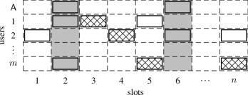
(a) Users’ transmissions in a B-CSA system. Rectangles represent transmitted packets. The time slots in which user $\mathsf{A}$ cannot receive are shown with gray. Erased packets due to the PEC are shown with hatched rectangles.

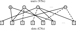
(b) Original graph $\tilde{\mathcal{G}}$. The dashed lines correspond to the packets erased due to the PEC, i.e., the solid lines show the PEC induced graph $\mathcal{G}$.

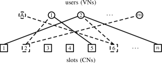
(c) PEC induced graph $\mathcal{G}$. The dashed lines show the nodes and the packets erased due to broadcast, i.e., solid lines show the broadcast induced graph $\mathcal{G}^{(r)}$ for user $\mathsf{A}$.

Figure 1: System model.

The main difference of the proposed B-CSA protocol compared to unicast CSA is that every user is also a receiver. Whenever a user does not transmit, it buffers the received signal. Without loss of generality, we focus on the performance of a single user, denoted by $\mathsf{A}$, also referred to as the receiver. $\mathcal{U}$ denotes the set of the other $m$ users, termed neighbors of user $\mathsf{A}$.

Since the frames are independent, it is sufficient to analyze the system within one frame. The received signal buffered by user $\mathsf{A}$ in slot $i$ is

$$y_{i}=\sum_{j\in\mathcal{U}_{i}}h_{i,j}a_{j},$$

where $a_{j}$ is a packet of the $j$-th user in $\mathcal{U}$, $h_{i,j}$ is the channel coefficient between user $j$ and the receiver, and $\mathcal{U}_{i}\subset\mathcal{U}$ is the set of user $\mathsf{A}$’s neighbors that transmit in the $i$-th slot.

The $i$-th slot is called a singleton slot if it contains only one packet. If it contains packets from more that one user, we say that a collision occurs in the $i$-th slot. Decoding proceeds as follows. First, user $\mathsf{A}$ decodes the packets in singleton slots and obtains the location of their copies. We assume decoding is possible if the corresponding channel coefficient satisfies $|h_{i,j}|>C$, where $C$ is a threshold that depends on the physical layer implementation. If $|h_{i,j}|\leq C$, we assume that the packet is erased, i.e., it cannot be decoded and does not cause any interference. The channel coefficients are assumed to be independent across users and slots and identically distributed such that $\mathrm{Pr}\left\{|h_{i,j}|\leq C\right\}=\epsilon$ and $\mathrm{Pr}\left\{|h_{i,j}|>C\right\}=1-\epsilon$, i.e., $\epsilon$ is the probability of a packet erasure. We refer to such a channel as a PEC. Using data-aided methods [25], the channel coefficients corresponding to the copies are then estimated. After subtracting the interference caused by the identified copies, decoding proceeds until no further singleton slots are found. We assume perfect interference cancellation, which is justified by physical layer simulation results in [4, 8]. We remark that decoding is always performed in singleton slots, such that the code rates of different users do not have to satisfy the rate constraint for joint decoding [26].

The system can be represented by a bipartite graph and can be analyzed using the theory of codes on graphs [8]. In the graph, each user corresponds to a variable node (VN) and represents a repetition code, whereas slots correspond to check nodes (CNs) and can be seen as single parity-check codes. In the following, the terms “users” and “VNs” are used interchangeably. A bipartite graph is defined by $\mathcal{G}=({\mathcal{V}},{\mathcal{C}},{\mathcal{E}})$, where $\mathcal{V}$, $\mathcal{C}$, and $\mathcal{E}$ represent the sets of VNs, CNs, and edges connecting them, respectively. The number of edges connected to a node is called the node degree. An important parameter in the graph is the VN degree distribution  [27, 28, 8]

$$\lambda(x)=\sum_{l=0}^{q}\lambda_{l}x^{l},$$ (1)

where $\lambda_{l}$ is the probability of a VN to have a degree $l$ (i.e., the probability that the user transmits $l$ copies of its packet) and $q$ is the maximum degree. We define a vector representation of (1) as $\bm{{\lambda}}=[{\lambda}_{0},\dots,{\lambda}_{q}]$. Furthermore, we define the graph profile as the vector $\bm{v}(\mathcal{G})=[v_{0}(\mathcal{G}),v_{1}(\mathcal{G}),\dots,v_{q}(\mathcal{G})]$, where $v_{l}(\mathcal{G})$ is the number of degree-$l$ VNs in $\mathcal{G}$. The total number of VNs in $\mathcal{G}$ is denoted by $\nu(\mathcal{G})$ and the total number of CNs is denoted by $\mu(\mathcal{G})$, i.e., $\nu(\mathcal{G})=m$ and $\mu(\mathcal{G})=n$.

In this paper, we focus on the broadcast packet loss rate (PLR), defined as the probability that a user in $\mathcal{U}$ is not resolved by the receiver. Since all users are independent, the PLR can be calculated as

$$\mathrm{bar}{p}=\frac{\mathrm{bar}{w}}{m},$$ (2)

where $\mathrm{bar}{w}$ is the average number of users that are not successfully decoded by user $\mathsf{A}$, termed unresolved users. Note that the PLR gives the probability that a packet of a user is not successfully received within a frame and does not refer to the copies sent by the user. We define the channel load as the ratio of contending users and the number of slots, i.e., $g=(m+1)/n$. It should be noted that, in the unicast scenario, the channel load is calculated as $g=m/n$, since the receiver is not contending.

III Induced Distribution and Packet Loss Rate

For transmission over a PEC, we showed in [21] that the performance of unicast CSA can be accurately approximated based on an induced distribution (ID) observed by the receiver. The fact that users in B-CSA cannot receive in the slots they use for transmission can also be modeled as packet erasures. Therefore, its performance can also be analyzed by means of the ID. In this section, we derive the ID in the general case of B-CSA over the PEC. To this end, we first find the degree distribution after the PEC and then the degree distribution perceived by user $\mathsf{A}$. Throughout the paper, $l$ and $d$ denote the original and the induced degrees of a user in $\mathcal{U}$, respectively, and $r$ denotes the degree of the receiver.

III-A Induced Distribution

For B-CSA over the PEC, three different graphs can be defined. The first one is the original graph, denoted by $\tilde{\mathcal{G}}$, that contains the edges $\tilde{\mathcal{E}}=\{e_{i,j}:1\leq i\leq n,\,\forall j\in\mathcal{U}_{i}\}$. We call its degree distribution the original distribution (the one used by the users for transmission) and denote it by $\tilde{\lambda}(x)$. The original graph corresponds to that of unicast CSA [8] and its distribution is in the hands of the system designer.

The PEC induced graph, denoted by $\mathcal{G}$, includes only the edges $e_{i,j}\in\tilde{\mathcal{E}}$, for which $|h_{i,j}|>C$. In other words, $\mathcal{G}$ is obtained from $\tilde{\mathcal{G}}$ by removing the edges corresponding to the erased packets. Since all elements of $\mathcal{G}$ are contained in $\tilde{\mathcal{G}}$, we call $\mathcal{G}$ a subgraph of $\tilde{\mathcal{G}}$ and write $\mathcal{G}\subset\tilde{\mathcal{G}}$ [29, Ch. 1.4]. The VN degree distribution of the PEC induced graph is called the PEC ID and is denoted by $\lambda(x)$. The graph $\mathcal{G}$ is what a base station in unicast CSA would observe after the PEC. However, only part of this graph is available to user $\mathsf{A}$ due to the half-duplex operation. Assuming that user $\mathsf{A}$ selects degree $r$, we denote its available subgraph by $\mathcal{G}^{(r)}$ and call it a broadcast induced graph. $\mathcal{G}^{(r)}$ can be obtained from $\mathcal{G}$ by removing the $r$ CNs corresponding to the slots where user $\mathsf{A}$ transmits and their adjacent edges. We call the degree distribution of this graph the broadcast ID and denote it by $\lambda^{(r)}(x)$. The number of check nodes in the broadcast induced graph, $n^{(r)}=\mu(\mathcal{G}^{(r)})=n-r$, is called the induced frame length. For the example in Fig. 1(a), $\tilde{\mathcal{G}}$, $\mathcal{G}$, and $\mathcal{G}^{(r)}$ are shown in Figs. 1(b) and 1(c).

We now derive the PEC ID. Let a user from the set $\mathcal{U}$ repeat its packet $l$ times. Each copy of this packet is erased with probability $\epsilon$. Hence, its degree in graph $\mathcal{G}$ is $k\leq l$ with probability $\binom{l}{k}\epsilon^{l-k}(1-\epsilon)^{k}$. Averaging over the original distribution $\tilde{\lambda}(x)$ leads to the PEC ID

$$\lambda(x)=\sum_{l=0}^{q}\tilde{\lambda}_{l}\sum_{k=0}^{l}\binom{l}{k}\epsilon^{l-k}(1-\epsilon)^{k}x^{k},$$

which can be written in the standard form (1), where

$$\lambda_{l}=\sum_{k=l}^{q}\binom{k}{l}\epsilon^{k-l}(1-\epsilon)^{l}\tilde{\lambda}_{k}.$$ (3)

Note that $\lambda_{l}$ is the fraction of users of degree $l$ after the PEC.

Assuming that user $\mathsf{A}$ selects degree $r$, another user that has degree $l$ after the PEC is perceived by user $\mathsf{A}$ as a degree-$d$ user if its non-erased transmissions take place in $l-d$ slots that are also selected by user $\mathsf{A}$, which occurs with probability $\binom{n-r}{d}\binom{r}{l-d}/\binom{n}{l}$. Given the constraint $0\leq l-d\leq r$, the broadcast ID $\lambda^{(r)}(x)$ observed by user $\mathsf{A}$ can be written as

$$\lambda^{(r)}(x)=\sum_{d=0}^{q}\lambda^{(r)}_{d}x^{d},$$

where

$$\lambda^{(r)}_{d}=\sum_{l=d}^{\min\{q,r+d\}}\frac{\binom{n-r}{d}\binom{r}{l-d}}{\binom{n}{l}}\lambda_{l}$$ (4)

is the fraction of users of degree $d$ as observed by user $\mathsf{A}$ if it selects degree $r$. Clearly, the broadcast ID depends on $n$, as opposed to the original and the PEC IDs. The IDs in [21, eq. (5)] and [30, eq. (3)] are a special case of (4) when $r=0$ and $\epsilon=0$, respectively.

Example 1.

For the original distribution

$$\tilde{\lambda}(x)=0.5x^{2}+0.5x^{4},$$ (5)

the PEC ID for $\epsilon=0.01$ is

$$\lambda(x)=0.00005+0.0099x+0.49x^{2}+0.019x^{3}+0.48x^{4}.$$ (6)

The broadcast IDs depend on $n$. For $n=100$, the broadcast IDs are

$$\lambda^{(2)}(x) =0.0004+0.03x+0.47x^{2}+0.06x^{3}+0.44x^{4},$$ (7)

$$\lambda^{(4)}(x) =0.001+0.05x+0.46x^{2}+0.09x^{3}+0.41x^{4}.$$ (8)

for a receiver degree 2 and 4, respectively.  $\triangle$

The coefficient in front of $\lambda_{l}$ in (4) can be written as

$$\frac{(n-r)!(n-l)!}{n!(n-r-d)!}\frac{r!l!}{d!(r-l+d)!(l-d)!}\propto n^{d-l},$$

i.e., it tends to zero as $n\to\infty$ if $l>d$. Since $l\geq d$, it can be shown that for any finite $r$, $\lambda_{d}^{(r)}=\lambda_{d}$ for all $r$ and $d$ when $n\rightarrow\infty$, i.e., $\lambda^{(r)}(x)\approx\lambda(x)$. This means that the effect of the broadcast nature of communications is negligible if the number of slots is large enough. However, when the number of slots is small, which is the case in delay critical applications, the difference between the PEC ID and the broadcast ID is significant, especially if $r$ is large.

III-B Packet Loss Rate

Let $p_{d}^{(r)}$ denote the probability that a user with degree $d$ in the broadcast induced graph $\mathcal{G}^{(r)}$ is not resolved by a receiver of degree $r$. We refer to $p_{d}^{(r)}$ as the degree-$d$ PLR. It can be calculated as

$$p_{d}^{(r)}=\frac{\mathrm{bar}{w}^{(r)}_{d}}{\mathrm{bar}{m}^{(r)}_{d}}=\frac{\mathrm{bar}{w}^{(r)}_{d}}{m\lambda^{(r)}_{d}},$$ (9)

where $\mathrm{bar}{m}^{(r)}_{d}$ and $\mathrm{bar}{w}^{(r)}_{d}$ are the average number of total and unresolved users of degree $d$ in $\mathcal{G}^{(r)}$, respectively. For $d=0$, $p_{0}^{(r)}=1$ and $\mathrm{bar}{w}^{(r)}_{0}=m\lambda^{(r)}_{0}$. For other degrees, we show how $\mathrm{bar}{w}^{(r)}_{d}$ can be approximated based on the broadcast ID in the next section. The probability that a degree-$r$ receiver cannot resolve a user is called the average PLR and can be obtained by averaging (9) over the broadcast ID as

$$p^{(r)}=\sum_{d=0}^{q}\lambda_{d}^{(r)}p_{d}^{(r)}.$$ (10)

The probability that the original degree-$l$ user is not resolved by a degree-$r$ receiver can be obtained as

$$\tilde{p}_{l}^{(r)} =\sum_{k=0}^{l}\binom{l}{k}\epsilon^{l-k}(1-\epsilon)^{k}\sum_{d=\mathrm{max}\{k-r,0\}}^{k}\frac{\binom{n-r}{d}\binom{r}{k-d}}{\binom{n}{k}}p_{d}^{(r)},$$ (11)

by reversing the operations in (3)–(4). Finally, the broadcast PLR in (2) is obtained as

$$\mathrm{bar}{p}=\sum_{r=0}^{q}\tilde{\lambda}_{r}p^{(r)}.$$ (12)

From the equations above it is clear that the performance of a B-CSA system depends on both the receiver and the transmitter degrees. We call this property DUEP and formalize it in the following lemmas.

Lemma 1.

For a given original distribution $\tilde{\lambda}(x)$ and any $n$, $\tilde{p}_{l}^{(\hat{r})}\geq\tilde{p}_{l}^{(r)}$ if $\hat{r}>r$.

Proof:

We prove the lemma by contradiction. Assume that the opposite holds, i.e., $\tilde{p}_{l}^{(\hat{r})}<\tilde{p}_{l}^{(r)}$ if $\hat{r}>r$. This implies that a degree-$r$ receiver can improve its performance by ignoring $(\hat{r}-r)$ randomly selected slots, which cannot be true, as ignoring the slot information is the worst possible way to use the slot. This leads to a contradiction. ∎

Lemma 1 describes the DUEP from the receiver perspective. The DUEP from the transmitter perspective is discussed in Lemma 2 in the following section.

IV Finite Frame Length Analysis

From (9)–(12) it follows that the degree-$d$ PLR $p_{d}^{(r)}$ is sufficient to describe all performance metrics for B-CSA. $p_{d}^{(r)}$ only depends on the distribution $\lambda^{(r)}(x)$ and the induced frame length $n^{(r)}$ seen by the receiver. The nature of these parameters is immaterial for the performance analysis. The receiver can be a user in a broadcast scenario that sees the broadcast ID $\lambda^{(r)}(x)$. Alternatively, it can be thought of as a receiver in a unicast scenario in which the contending users use $\lambda^{(r)}(x)$ as the original distribution with the frame length $n^{(r)}$. Therefore, for the sake of simplicity, in this section we consider a unicast scenario, we omit superscript $(r)$ and analyze $p_{d}$ in (9) for frame length $n$ and an arbitrary distribution $\lambda(x)$ used to generate graph $\mathcal{G}$.

For $n\to\infty$, the typical performance of CSA exhibits a threshold behavior, i.e., all users are successfully resolved if the channel load is below a certain threshold value, which can be obtained via density evolution (DE) [8]. The threshold, denoted by $g^{*}(\bm{\lambda})$, depends only on the degree distribution $\lambda(x)$. We use the analysis in [8] to describe the DUEP from the transmitter perspective in the following lemma.

Lemma 2.

For a given distribution $\lambda(x)$, any load $0<g\leq 1$, and sufficiently large $n$, $p_{\hat{d}}<p_{d}$ if $\hat{d}>d$.

Proof:

We denote the degree-$d$ PLR at the $\rho$-th decoding iteration, $\rho\geq 1$, as a function of $n$ by $p_{d}(n,\rho)$. According to the analysis in [8, 31],

$$\lim_{n\to\infty}p_{d}(n,\rho)=(\xi_{\rho})^{d}$$ (13)

for any finite $d$, where $\xi_{\rho}$ is the probability of not removing an edge at the $\rho$-th decoding iteration. This probability is obtained recursively as [8, Sec. III]

$$\xi_{\rho}=1-\exp{\left(-g\lambda^{\prime}(\xi_{\rho-1})\right)},$$ (14)

where the prime denotes the derivative and $\xi_{0}=1$. (13) asserts that for any $\theta>0$ there exists an $n$ such that

$$(\xi_{\rho})^{d}-\theta\leq p_{d}(n,\rho)\leq(\xi_{\rho})^{d}+\theta.$$ (15)

It is easy to show from (14) that $\xi_{\rho}<1$ for $0<g\leq 1$ and any $\rho\geq 1$. Hence, $(\xi_{\rho})^{\hat{d}}<(\xi_{\rho})^{d}$ and we can always find $\theta>0$ such that $(\xi_{\rho})^{\hat{d}}+\theta<(\xi_{\rho})^{d}-\theta$. Thus, according to (15) there exists an $n$ such that $p_{\hat{d}}<p_{d}$ at any iteration. ∎

Remark 1.

In practice, it is sufficient that $n\gg q$ to guarantee $p_{\hat{d}}<p_{d}$ if $\hat{d}>d$.

Lemma 2 states that users that transmits more have a higher probability of being decoded by the receiver for sufficiently large frame lengths. The finite frame length regime gives rise to an EF in the PLR performance of CSA. This EF is due to stopping sets in the graph $\mathcal{G}$. In this section, we first define stopping sets and analyze their contribution to the PLR. We then identify the stopping sets that contribute the most to the EF and propose an analytical approximation to the performance in the EF region.

IV-A Stopping Sets and Their Contribution to Packet Loss Rate

Since erased packets are accounted for in the ID, the only source of errors in the considered model is represented by the harmful structures in the graph $\mathcal{G}$. For example, when two degree-$2$ users transmit in the same slots (see Fig. 2(a)), the receiver is not able to resolve them. Such harmful structures are commonly referred to as stopping sets [16].

Definition 1.

A connected bipartite graph $\mathcal{S}$ is a stopping set if all CNs in $\mathcal{S}$ have a degree larger than one.

We say that a stopping set $\mathcal{S}$ has profile $\bm{v}(\mathcal{S})$ and contains $\nu(\mathcal{S})$ VNs and $\mu(\mathcal{S})$ CNs. For example, for the stopping set in Fig. 2(a), the graph profile is $\bm{v}(\mathcal{S})=[0,0,2,0,\dots,0]$, where the number of zeros in the end depends on $q$, $\nu(\mathcal{S})=2$, and $\mu(\mathcal{S})=2$. Stopping sets are referred to as “loops” in [24]. However, stopping sets do not necessarily form a loop if degree-$1$ users are present. To analyze stopping sets, we define a VN-induced graph as follows.

(a) Stopping set $\mathcal{S}$.

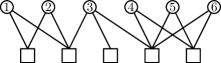
(b) Graph $\mathcal{G}$.

Figure 2: Number of stopping sets $\mathcal{S}$ in graph $G$.

Definition 2.

A graph consisting of a subset of VNs of a graph $\mathcal{G}$ and all their neighbors is called a VN-induced graph.

Since the graph $\mathcal{G}$ and its profile $\bm{v}(\mathcal{G})$ are random, the average number of unresolved degree-$d$ users in (9) can be expressed using stopping sets as

$$\mathrm{bar}{w}_{d}=\mathsf{E}_{\mathcal{G}}\left\{\sum_{\mathcal{S}\in\mathcal{A}}v_{d}(\mathcal{S})\hat{w}(\mathcal{S},\mathcal{G})\right\},$$ (16)

where $\mathcal{A}$ is the set of all possible stopping sets for given $n$ and $m$, $v_{d}(\mathcal{S})$ is the number of degree-$d$ VNs in $\mathcal{S}$, and $\mathsf{E}_{x}\left\{\cdot\right\}$ denotes the expectation over the random variable $x$. $\hat{w}(\mathcal{S},\mathcal{G})$ in (16) is the number of VN-induced graphs in a graph realization $\mathcal{G}$ which are both: i) isomorphic with $\mathcal{S}$ [32, Ch. 16.9]; ii) not a subgraph of a VN-induced graph isomorphic with another stopping set in $\mathcal{A}$. With a slight abuse of notation, we refer to $\hat{w}(\mathcal{S},\mathcal{G})$ as the number of stopping sets $\mathcal{S}$ in a graph $\mathcal{G}$. The following example explains the definition of $\hat{w}(\mathcal{S},\mathcal{G})$.

Example 2.

Consider the stopping set $\mathcal{S}$ in Fig. 2(a) and the graph $\mathcal{G}$ in Fig. 2(b). There are three VN-induced graphs in $\mathcal{G}$ isomorphic with $\mathcal{S}$, namely, the graphs induced by VNs $\{1,2\}$, $\{4,5\}$, and $\{5,6\}$. However, the two latter ones are subgraphs of another VN-induced graph isomorphic with a larger stopping set induced by the VNs $\{4,5,6\}$. Hence $\hat{w}(\mathcal{S},\mathcal{G})=1$.

The averaging in (16) can be done in two steps as

$$\mathrm{bar}{w}_{d}=\mathsf{E}_{\bm{v}(\mathcal{G})}\left\{\sum_{\mathcal{S}\in\mathcal{A}}v_{d}(\mathcal{S})w(\mathcal{S},\mathcal{G})\right\},$$ (17)

where

$$w(\mathcal{S},\mathcal{G})=\mathsf{E}_{\hat{\mathcal{G}}:\bm{v}(\hat{\mathcal{G}})=\bm{v}(\mathcal{G})}\left\{\hat{w}(\mathcal{S},\hat{\mathcal{G}})\right\}$$

is the average number of stopping sets $\mathcal{S}$ in graphs with a particular profile $\bm{v}(\mathcal{G})$.

From the definition of a stopping set it follows that, for a given profile $\bm{v}(\mathcal{G})$, the number of stopping sets can be expressed as

$$w(\mathcal{S},\mathcal{G})=\alpha(\mathcal{S},\mathcal{G})\beta(\mathcal{S})\gamma(\mathcal{S})\delta(\mathcal{S},\mathcal{G}),$$ (18)

where

$$\alpha(\mathcal{S},\mathcal{G})=\prod_{d=1}^{q}\binom{v_{d}(\mathcal{G})}{v_{d}(\mathcal{S})}$$ (19)

is the number of ways to select VNs needed to create $\mathcal{S}$ in a graph with profile $\bm{v}(\mathcal{G})$ and

$$\beta(\mathcal{S})=\binom{n}{\mu(\mathcal{S})}$$ (20)

is the number of ways to select $\mu(\mathcal{S})$ CNs out of $n$ CNs. $\gamma(\mathcal{S})$ in (18) is the probability of the selected VNs to be connected to the selected CNs so that $\mathcal{S}$ is created. $\gamma(\mathcal{S})$ can be written as the ratio of the number of stopping sets $\mathcal{S}$ that the selected VNs can create over the total number of graphs they can create, i.e.,

$$\gamma(\mathcal{S})=\frac{c(\mathcal{S})}{\prod_{d=1}^{q}\binom{n}{d}^{v_{d}(\mathcal{S})}},$$ (21)

where $c(\mathcal{S})$ is the number of graphs isomorphic with $\mathcal{S}$ that the selected VNs can create. Unfortunately, deriving a closed-form expression for this constant does not seem to be straightforward. However, it can be found numerically according to its definition, as demonstrated in the following example.

Example 3.

To find $c(\mathcal{S})$, we need to enumerate all combinations of connecting the VNs in $\mathcal{S}$ to the CNs in $\mathcal{S}$ so that the resulting graph is isomorphic with $\mathcal{S}$. Consider stopping set $\mathcal{S}$ in Fig. 3(a). The only two graphs that are isomorphic with $\mathcal{S}$ are shown in Figs. 3(b) and 3(c). Hence, $c(\mathcal{S})=3$. To find $c(\mathcal{S})$, all graphs with a given profile $v(\mathcal{S})$ need to be generated and their isomorphism with $\mathcal{S}$ tested [32, Ch. 16.9].  $\triangle$

(a)

(b)

(c)

Figure 3: Isomorphic graphs for a stopping set in (a).

$\delta(\mathcal{S},\mathcal{G})$ in (18) is the probability that the other $m-\nu(\mathcal{S})$ VNs are connected to CNs in such a way that another stopping set $\hat{\mathcal{S}}\supset\mathcal{S}$ is not created (see Fig. 2). It does not have a closed-form expression in general and we resort to an upper bound. By setting $\delta(\mathcal{S},\mathcal{G})=1$ in (18), substituting the result into (17) and bringing the expectation inside the summation, we obtain the upper bound given by

$$\mathrm{bar}{w}_{d}\leq{\sum_{\mathcal{S}\in\mathcal{A}}v_{d}(\mathcal{S})\alpha(\mathcal{S})\beta(\mathcal{S})\gamma(\mathcal{S})},$$ (22)

where $\alpha(\mathcal{S})=\mathsf{E}_{\bm{v}(\mathcal{G})}\left\{\alpha(\mathcal{S},\mathcal{G})\right\}$, which can be expressed as [21]

$$\alpha(\mathcal{S})=\frac{m!}{(m-\nu(\mathcal{S}))!}\prod_{d=1}^{q}\frac{\lambda_{d}^{v_{d}(\mathcal{S})}}{v_{d}(\mathcal{S})!}.$$ (23)

The upperbound in (22) can be seen as a union bound, in which the occurrences of stopping sets are no longer exclusive events.

We now show that the bound in (22) is tight for large $n$. $\delta(\mathcal{S},\mathcal{G})$ in (18) can be lower-bounded by the probability that none of these VNs is connected to the selected CNs. For a user of degree $d$, the probability of not being connected to the selected CNs is $\frac{\binom{n-\mu(\mathcal{S})}{d}}{\binom{n}{d}}$ for $n\geq d+\mu(\mathcal{S})$, which together with the expression for the binomial coefficient gives

$$\delta(\mathcal{S},\mathcal{G})\geq\prod_{d=1}^{q}\left(\prod_{k=0}^{d-1}\frac{n-\mu(\mathcal{S})-k}{n-k}\right)^{(v_{d}(\mathcal{G})-v_{d}(\mathcal{S}))^{+}},$$ (24)

where $x^{+}=\mathop{\mathrm{max}}{(}0,x)$ and $n\geq q+\mu(\mathcal{S})$ (since the inequality $n\geq d+\mu(\mathcal{S})$ has to hold for any $d$). A looser lower bound can be obtained additionally assuming that all these VNs have degree $q$,

$$\delta(\mathcal{S},\mathcal{G}) \geq\left(\prod_{k=0}^{q-1}\frac{n-\mu(\mathcal{S})-k}{n-k}\right)^{(m-\nu(\mathcal{S}))^{+}}$$

$$\geq\prod_{k=0}^{q-1}\left(\frac{n-\mu(\mathcal{S})-q+1}{n-q+1}\right)^{(m-\nu(\mathcal{S}))^{+}}$$

$$=\left(1-\frac{\mu(\mathcal{S})}{n-q+1}\right)^{q(m-\nu(\mathcal{S}))^{+}}$$

$$\geq\left(1-\frac{\mu(\mathcal{S})}{n-q+1}\right)^{qm}$$

$$\geq\exp{\left(-\frac{q\mu(\mathcal{S})m}{n-q+1-\mu(\mathcal{S})}\right)},$$ (25)

where the last step follows from the inequality $\log(x)\geq 1-1/x$ for $x>0$. From (25) it follows that, for large $n$ ($n\gg q+\mu(\mathcal{S})$) and low channel loads ($n\gg q\mu(\mathcal{S})m$), $\delta(\mathcal{S},\mathcal{G})\approx 1$, which shows that (22) is tight for large $n$.

Example 4.

For the distribution $\lambda(x)=x$ (slotted ALOHA), i.e., all VNs have degree 1, all factors in (18) can be easily calculated and the exact expression for (17) can be obtained. Since all VNs have degree 1, the profile of $\mathcal{G}$ is deterministic with $\bm{v}(\mathcal{G})=[0,\,m]$, and the expectation in (17) is trivial. Furthermore, all stopping sets have one CN with $s$, $2\leq s\leq m$, VNs connected to it. Such a stopping set, denoted by $\mathcal{S}_{s}$, has parameters

$$\bm{v}(\mathcal{S}_{s})=[0,\,s],\quad\mu(\mathcal{S}_{s})=1,\quad\alpha(\mathcal{S}_{s},\mathcal{G})=\binom{m}{s},$$

$$\beta(\mathcal{S}_{s})=\binom{n}{1},\,\gamma(\mathcal{S}_{s})=\phi^{s},\,\delta(\mathcal{S}_{s},\mathcal{G})=(1-\phi)^{m-s},$$

where $\phi=1/n$. We remark that the expression for $\delta(\mathcal{S}_{s},\mathcal{G})$ coincides with the bound in (24) since the VNs ouside $\mathcal{S}_{s}$ cannot be connected to $\mathcal{S}_{s}$ without creating a larger stopping set and $c(\mathcal{S}_{s})=1$ for any $s$.

Since only degree-$1$ VNs are present in the graph, $\mathrm{bar}{w}_{1}$ (see (17)) can be calculated exactly as

$$\mathrm{bar}{w}_{1}=\sum_{s=2}^{m}s\binom{m}{s}\binom{n}{1}\phi^{s}(1-\phi)^{m-s}.$$ (26)

Finally, by using the properties of the binomial distribution, we can obtain the exact expression for the PLR in (10) as

$$p=p_{1}=\frac{\mathrm{bar}{w}_{1}}{m}=\frac{n}{m}\sum_{s=2}^{m}s\binom{m}{s}\phi^{s}(1-\phi)^{m-s}\\ =g^{-1}(m\phi-m\phi(1-\phi)^{m-1})=1-(1-\phi)^{ng-1},$$ (27)

which corresponds to the well known expression for the PLR of framed slotted ALOHA [33, eq. (3)].  $\triangle$

IV-B Dominant Stopping Sets and Error Floor Approximation

Identifying all stopping sets and calculating the corresponding $\gamma(\mathcal{S})$ in a systematic way for an arbitrary $n$ is not possible in general. We therefore determine stopping sets that contribute the most to the PLR for low channel loads, i.e., in the EF region. It is clear that, for low channel loads ($n\gg m$), stopping sets with a small number of nodes are more likely to occur. We therefore focus on stopping sets with few CNs. Furthermore, to reduce the number of considered stopping sets, we define minimal stopping sets as follows.

Definition 3.

A minimal stopping set is a stopping set that does not contain a nonempty stopping set of smaller size.

It can be seen from (20) and (21) that for low channel loads (more precisely, when $\sum_{d}dv_{d}(\mathcal{S})\ll n$), each edge in $\mathcal{S}$ gives a factor $n^{-1}$ in $\gamma$ and each CN gives a factor $n$ in $\beta(\mathcal{S})$. Assume now two stopping sets $\mathcal{S}$ and $\hat{\mathcal{S}}$ such that $\mathcal{S}\subset\hat{\mathcal{S}}$. To obtain $\mathcal{S}$ from $\hat{\mathcal{S}}$, more edges than CNs need to be removed from $\hat{\mathcal{S}}$ since each CN in $\hat{\mathcal{S}}$ is connected to at least two edges. Hence, the contribution of a non-minimal stopping set $\hat{\mathcal{S}}$ to the PLR is smaller than that of $\mathcal{S}$ for low channel loads. We therefore only consider minimal stopping sets in our analysis. Simulation results in Section V justify restricting to minimal stopping sets.

We run an exhaustive search of minimal stopping sets with $\mu(\mathcal{S})$ up to five. For $\mu(\mathcal{S})\leq 4$, there are 31 minimal stopping sets with the corresponding parameters given in Table I. For $\mu(\mathcal{S})=5$, there are 111 minimal stopping sets (not included in this paper). We remark that the complexity of finding $c(\mathcal{S})$ depends on the size of a stopping set [32, Ch. 16.9]. Therefore, we restrict the analysis to $\mu(\mathcal{S})\leq 4$. The most dominant stopping sets presented in [21] are a subset of the stopping sets in Table I. Considering more stopping sets can improve the PLR approximation for moderate channel loads.

TABLE I: Parameters of minimal stopping sets with $\mu(\mathcal{S})\leq 4$.

$\bm{v}(\mathcal{S})$	$\mu(\mathcal{S})$	$c(\mathcal{S})$
$[0,\,2,\,0,\,0,\,0]$	$1$	$1$
$[0,\,0,\,2,\,0,\,0]$	$2$	$1$
$[0,\,2,\,1,\,0,\,0]$	$2$	$2$
$[0,\,0,\,0,\,2,\,0]$	$3$	$1$
$[0,\,1,\,1,\,1,\,0]$	$3$	$3$
$[0,\,0,\,3,\,0,\,0]$	$3$	$6$
$[0,\,0,\,2,\,1,\,0]$	$3$	$6$
$[0,\,3,\,0,\,1,\,0]$	$3$	$6$
$[0,\,2,\,2,\,0,\,0]$	$3$	$12$
$[0,\,0,\,0,\,0,\,2]$	$4$	$1$
$[0,\,1,\,0,\,1,\,1]$	$4$	$4$
$[0,\,0,\,2,\,0,\,1]$	$4$	$6$
$[0,\,0,\,1,\,2,\,0]$	$4$	$12$
$[0,\,0,\,1,\,1,\,1]$	$4$	$12$
$[0,\,0,\,0,\,3,\,0]$	$4$	$24$

$[0,\,0,\,0,\,2,\,1]$	$4$	$12$
$[0,\,2,\,1,\,0,\,1]$	$4$	$12$
$[0,\,2,\,0,\,2,\,0]$	$4$	$24$
$[0,\,1,\,2,\,1,\,0]$	$4$	$24$
$[0,\,1,\,2,\,1,\,0]$	$4$	$24$
$[0,\,1,\,2,\,0,\,1]$	$4$	$24$
$[0,\,1,\,1,\,2,\,0]$	$4$	$48$
$[0,\,0,\,3,\,1,\,0]$	$4$	$24$
$[0,\,0,\,3,\,0,\,1]$	$4$	$24$
$[0,\,0,\,4,\,0,\,0]$	$4$	$72$
$[0,\,0,\,3,\,1,\,0]$	$4$	$144$
$[0,\,0,\,2,\,2,\,0]$	$4$	$48$
$[0,\,0,\,2,\,2,\,0]$	$4$	$48$
$[0,\,4,\,0,\,0,\,1]$	$4$	$24$
$[0,\,3,\,1,\,1,\,0]$	$4$	$72$
$[0,\,2,\,3,\,0,\,0]$	$4$	$144$

Constraining the set of the considered stopping sets in (22) to minimal stopping sets with $\mu(\mathcal{S})\leq 4$ and combining it with (9) gives the following approximation of the degree-$d$ PLR in the EF region

$$p_{d}\approx\frac{1}{m\lambda_{d}}\sum_{\mathcal{S}\in\mathcal{A}_{31}}{v_{d}(\mathcal{S})\alpha(\mathcal{S})\beta(\mathcal{S})}\gamma(\mathcal{S}),$$ (28)

where $\mathcal{A}_{31}$ is the set of 31 minimal stopping sets in Table I with $\alpha(\mathcal{S})$, $\beta(\mathcal{S})$, and $\gamma(\mathcal{S})$ given in (23), (20), and (21), respectively. Since the considered stopping sets include VNs of degrees up to four, the approximation in (28) can only be used for $d\in\{1,\dots,4\}$. If the PLR for larger degrees needs to be estimated, the set of considered stopping sets should be extended.

We remark that, in practice, distributions with large fractions of low-degree VNs are most commonly considered since they achieve high thresholds. For instance, the soliton distribution [9], for which $g^{*}(\bm{\lambda})=1$, has $\lambda_{2}=0.5$ and $\lambda_{3}=0.17$ (and $\lambda_{0}=\lambda_{1}=0$). Moreover, IDs for B-CSA and/or the PEC have relatively high fractions of users of low degrees due to packet erasures. We therefore conclude that the approximation in (28) is accurate for estimating the average performance of most CSA systems of practical interest. This is supported by extensive numerical simulations, some of which are presented in the next section.

V Numerical Results

In this section, we first present different aspects of the B-CSA performance for the distributions in Example 1. We then show how the proposed EF approximation can be used for the optimization of the original distribution.

V-A Induced Distribution and Packet Loss Rate

In Fig. 4, we show the simulated PLRs $p_{d}^{(r)}$ and $\tilde{p}_{l}^{(r)}$ (solid lines) for the system described in Example 1. Fig. 4(a) shows the PLR for users of different induced degrees and illustrates the DUEP property. Lines with circles show $p_{d}^{(2)}$ for the distribution in (7) and lines with diamonds show $p_{d}^{(4)}$ for the distribution in (8) and $d=1,\dots,4$. It can be seen that for a given distribution, the larger the transmitter degree $d$, the better the performance, as Lemma 2 states.

Fig. 4(b) shows the simulated PLR $\tilde{p}_{l}^{(r)}$ for the original transmitter degree $l$. As it can be seen from the figure, for a given $l$, the receiver with a smaller degree $r$ has better performance in accordance with Lemma 1. On the other hand, for a given $r$, the transmitter with a smaller degree $l$ has worse performance. The rationale behind the DUEP is that the chance of a user to be resolved by other users increases if the user transmits more, but at the same time the chance to resolve other users decreases.

We remark that the curves for $\tilde{p}_{l}^{(r)}$ in Fig. 4(b) can be alternatively obtained from the solid curves in Fig. 4(a) via (11). The resulting curves would then appear exactly on top of the simulation results in Fig. 4(b), which confirms the correctness of (11) and the derived IDs.

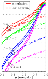
(a) $p_{d}^{(r)}$.

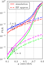
(b) $\tilde{p}_{l}^{(r)}$.

Figure 4: PLR performance of B-CSA for the scenario in Example 1 ($n=100$). Solid curves show simulation results and dashed curves show analytical EF approximations. Circles and diamonds show the PLR for $r=2$ and $r=4$, respectively.

V-B Error Floor Approximation

Fig. 4 also shows the proposed analytical EF approximation (28) (dashed lines). Fig. 4(a) shows (28) for the distribution in (7), $r=2$ and $d=1,2,3,4$, whereas Fig. 4(b) shows (11) used together with the approximation (28) for $l=2,4$ and $r=2,4$. The analytical EF approximations demonstrate good agreement with the simulation results for low to moderate channel loads. This justifies the approximation in (28) and the use of minimal stopping sets. It can also be seen that the approximations for $d=1,2$ are more accurate than those for $d=3,4$ since the stopping sets in Table I contain mostly users of low degrees.

Fig. 5 shows the dependency of the EF on the frame length for the distributions in (5) and (6), which correspond to $\epsilon=0$ and $\epsilon=0.01$, respectively, in the unicast scenario. It can be observed that without channel erasures (green curve), the EF decays exponentially with $n$. When erasures are present (red curve), the performance first decays exponentially for small $n$ and then approaches the value predicted by DE (black dot) as $n$ grows. For $n\lessapprox 10^{3}$, the finite frame length is the main cause of the EF, whereas for $n\gtrapprox 10^{3}$ the PEC is the dominant factor causing the EF. In this case, increasing $n$ does not improve the performance. Markers show simulation results, which agree well with the analytical approximation.

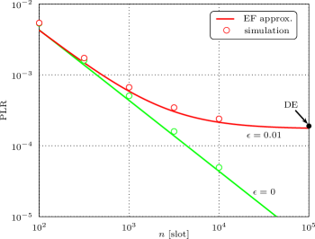
Figure 5: PLR performance of unicast CSA versus $n$ for the distributions in (5)–(6) and $g=0.5$. Solid lines show the analytical approximation (28) with (11) and markers show simulation results. The PLR value $2\cdot 10^{-4}$ predicted by DE is shown with a black dot.

Finally, in Fig. 6 we show how the proposed EF approximation compares with the DE results for large $n$. The solid lines show the PLR $\lim_{n\to\infty}p_{d}(n,\infty)$ obtained via DE (13) for the distribution in (6) and $d=1,\dots,4$ in the unicast scenario. The proposed EF approximation (28) for $n=10^{7}$ is shown with dashed lines and agrees well with the DE curves. The lower the degree, the larger the range of channel loads for which the agreement is good. We remark that in all considered examples, the proposed analytical EF approximation always underestimates the PLR. This can be improved by including more stopping sets in (28).

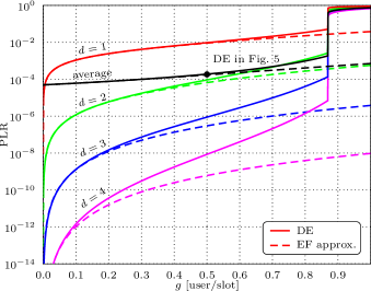
Figure 6: PLR performance of unicast CSA with the distribution in (6) and $n=10^{7}$. Solid lines show the PLR predicted by DE and dashed lines show the proposed EF approximation.

V-C Distribution Optimization for All-to-All Broadcast Coded Slotted ALOHA

In this subsection, we concentrate on the broadcast scenario and discuss the optimization of the degree distribution for finite frame lengths using the proposed EF approximation. To this end, we constrain the original distribution to have the form $\tilde{\lambda}(x)=\tilde{\lambda}_{2}x^{2}+\tilde{\lambda}_{3}x^{3}+\tilde{\lambda}_{4}x^{4}+\tilde{\lambda}_{8}x^{8}$. Such distributions have a good performance in the unicast scenario [8] and are typical for low-density parity-check codes [34, p. 397].

Ideally, we would like to minimize the PLR around the values of $g$ at which the PLR curve switches from the waterfall region to the EF region. However, analytical tools to predict the PLR at such channel loads are missing. The proposed EF approximation (28) is accurate only for low to moderate channel loads. If the EF approximation is the only optimization objective, the optimal distribution is always $\tilde{\lambda}(x)=x^{8}$. However, such a distribution has $g^{*}(\bm{\lambda})=0.54$, hence, bad performance at channel loads of interest. Here, we use a linear combination of the broadcast PLR in (12) and the threshold as the optimization objective, which corresponds to scalarization of a multidimensional objective function [35, Ch. 4.7].

For notational convenience, we write the broadcast PLR in (12) as $\mathrm{bar}{p}(\bm{\tilde{\lambda}})$ to highlight that it depends on the distribution $\bm{\tilde{\lambda}}$ and formulate the following optimization problem

$$\underset{\bm{\tilde{\lambda}}}{\text{minimize}} -g^{*}(\bm{\tilde{\lambda}})+\eta\mathrm{bar}{p}(\bm{\tilde{\lambda}})$$

subject to $$\tilde{\lambda}_{i}\geq 0\;i=2,3,4,8,$$

$$\tilde{\lambda}_{i}=0\;\text{otherwise},$$

$$\tilde{\lambda}_{2}+\tilde{\lambda}_{3}+\tilde{\lambda}_{4}+\tilde{\lambda}_{8}=1,$$

where $\eta$ is a weighting coefficient. We numerically solve this optimization problem by using the EF approximation (28) to calculate $\mathrm{bar}{p}(\bm{\tilde{\lambda}})$ for different values of $\eta$ and obtain the EF vs. threshold tradeoff shown in Fig. 7(a). The corresponding optimal distributions are shown in Fig. 7(b). As it can be seen from Fig. 7(a), the optimal distributions around $g^{*}=0.85$ provide relatively high threshold for relatively low EF values ($\approx 10^{-5}$). We pick the distribution

$$\tilde{\lambda}(x) =0.86x^{3}+0.14x^{8}$$ (29)

and use it in the next section when we compare B-CSA with CSMA. We remark that the choice of $g^{*}$ for selecting the distribution depends on the required reliability. Since global optimality of the results in Fig. 7 is not guaranteed, better distributions can potentially be obtained. However, the presented distributions are the best known distributions that provide the EF vs. threshold tradeoff.

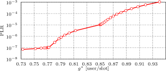
(a) EF vs. threshold tradeoff.

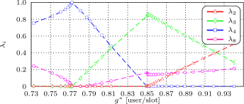
(b) Optimal distributions.

Figure 7: Distribution optimization for $n=500$, $g=0.5$, and $\epsilon=0$.

The results in Fig. 7 are obtained for $n=500$, $g=0.5$, and $\epsilon=0$. We remark that the distribution in (29) is close to the one presented in [21] for the unicast scenario. Furthermore, we observed that the optimization problem is not very sensitive to the choice of parameters $g$, $n$, and $\epsilon$.

VI Broadcast Coded Slotted ALOHA in Vehicular Networks

In this section, we evaluate the performance of B-CSA in a vehicular network and compare it with the currently used CSMA protocol. The physical layer parameters used here are taken from [37] and are given in Table II. We consider transmission of cooperative awareness message (CAM) [38] packets that are sent periodically every $t_{\text{frame}}$ seconds. We set the frame duration equal to $t_{\text{frame}}$ and we assume that the network does not change during this period. We assume that all packets have length $t_{\text{pack}}$, which depends on the packet size $d_{\text{pack}}$, transmission rate $r_{\text{data}}$, and the length of the preamble added to every packet $t_{\text{pream}}$, i.e., $t_{\text{pack}}=t_{\text{pream}}+d_{\text{pack}}/r_{\text{data}}$. In addition, the slot duration $t_{\text{slot}}=t_{\text{pack}}+t_{\text{guard}}$, where $t_{\text{guard}}$ accounts for timing inaccuracy. The number of slots is determined as $n=\lfloor t_{\text{frame}}/t_{\text{slot}}\rfloor$. The inclusion of a guard interval, $t_{\text{guard}}$, reduces the number of slots in a frame and thus worsens the performance of B-CSA.

TABLE II: The PHY parameters. The values in the upper part are taken from [37]; the values in the lower part are derived.

Parameter	Variable	Value		Units
Data rate	$r_{\text{data}}$	6		Mbps
PHY preamble	$t_{\text{pream}}$	40		$\mu$s
CSMA slot duration	$t_{\text{csma}}$	13		$\mu$s
AIFS time	$t_{\text{aifs}}$	58		$\mu$s
Frame duration	$t_{\text{frame}}$	100		ms
Guard interval	$t_{\text{guard}}$	5		$\mu$s
Packet size	$d_{\text{pack}}$	200	400	byte
Packet length	$t_{\text{pack}}$	312	576	$\mu$s
Slot duration	$t_{\text{slot}}$	317	581	$\mu$s
Number of slots	$n$	315	172

VI-A Carrier Sense Multiple Access

CSMA is used as MAC protocol for vehicular networks [37]. We analyze the following system model that can be compared with B-CSA. We consider a network with $m+1$ users indexed by $j=1,\dots,m+1$, where every user is within all other users transmission range, i.e., no collision occurs due to the hidden terminal problem. $m$ can be thought of as the instantaneous number of neighbors for a given user. We assume that a user can always sense other users transmissions. Collisions are assumed to be destructive. If no collision occurs, each user may not able to decode a packet with probability $\epsilon$ due to noise-induced errors. We say that such a packet is erased. Note that the backoff protocol is not affected by channel erasures and partial collisions are not possible.

The set of users is denoted by $\mathcal{V}$ and time is denoted by $t$. At the beginning of the contention ($t=0$), every user selects a real random number $\tau_{j}\in[0,\,\,t_{\text{frame}})$, which represents the time when the $j$-th user attempts to transmit its first packet invoking the CSMA procedure from [39, Fig. 2(a)]. The contention window size is selected to be 511 [30]. $t_{\text{aifs}}$ is the sensing period during which the users sense the channel to determine whether it is busy of not, where AIFS stands for arbitration interframe space. $t_{\text{csma}}$ is the duration of a backoff slot. The values of these parameters are specified in [37] (see Table II for the values used in simulations).

To overcome the effect of packet erasures, each user attempts $\kappa$ transmissions of each packet. At time instant $\tau_{j}+(k-1)t_{\text{frame}}/\kappa+(i-1)t_{\text{frame}}$, the $j$-th user makes the $k$-th attempt, $k=1,\dots,\kappa$, to transmit its $i$-th packet, $i=1,\,2,\,\dots$. If by the time $\tau_{j}+it_{\text{frame}}$ none of the copies of the $i$-th packet is transmitted, the packet is dropped. For $\kappa=1$, the described protocol is considered in [30].

The channel load is defined as the ratio of the number of users, $m+1$, and $t_{\text{frame}}$ (expressed in slots) to match the definition of the channel load for B-CSA, i.e., $g=(m+1)/(t_{\text{frame}}/t_{\text{slot}})=(m+1)/n$. The PLR for user $j$ is defined as

$$p_{j}=1-\frac{\mathsf{E}_{\tau_{1},\dots,\tau_{m}}\left\{\sum_{\begin{subarray}{c}i\in\mathcal{V}\\ i\neq j\end{subarray}}\eta_{i,j}\right\}}{m},$$

where $\eta_{i,j}\in\{0,1,2\}$ is the number of packets of user $i$ successfully received by user $j$ over the time interval $[t_{0},\,\,t_{0}+t_{\text{frame}})$. To estimate the performance, we introduce a time offset $t_{0}=2t_{\text{frame}}$ in order to remove the transient in the beginning of the contention. As the performance does not depend on the particular user, without loss of generality, we select user $j=1$.

The performance of CSMA for different values of $\epsilon$, $\kappa$, and the frame lengths in Table II is shown in Fig. 8. We can observe that the performance of CSMA degrades as $n$ increases due to the increase of sensing overhead. Furthermore, for a given $n$, increasing $\kappa$ reduces the achievable throughput but improves the performance at low channel loads. The PLR curves approach the value $\epsilon^{\kappa}$ for $g=0$, hence, the number of repetitions can be predicted based on $\epsilon$ and the required reliability.

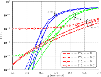
Figure 8: PLR performance for CSMA over the PEC. Solid and dashed lines correspond to $\epsilon=0$ and $\epsilon=0.01$, respectively. Circles and diamonds show the PLR for $n=172$ and $n=315$, respectively.

VI-B Carrier Sense Multiple Access vs. All-to-all Broadcast Coded Slotted ALOHA

Even though the reliability requirements are not specified in [37] and depend on the particular application, for the sake of comparison we assume that the broadcast PLR of interest is in the range $10^{-2}\,-\,10^{-3}$. From Fig. 8 it follows that for CSMA, $\kappa=2$ provides good performance for the PEC with $\epsilon\leq 10^{-2}$. For B-CSA we select the distribution in (29).

The broadcast PLR of the two protocols is shown in Fig. 9 for $n=172$ and $n=315$ (see Table II). Simulation results for B-CSA and CSMA are shown with solid and dashed lines, respectively. The dash-dotted lines show the broadcast PLR obtained using the approximation (28). The figure shows that the protocols react differently to the increase of the frame length: The CSMA performance degrades when $n$ increases whereas the performance of B-CSA improves as $n$ grows large. This gives an extra degree of freedom when designing a B-CSA system, as increasing the bandwidth will decrease the packet length and, hence, increase the number of slots. Moreover, B-CSA is robust to packet erasures for any channel load as opposed to CSMA, which suffers significantly at low channel loads. We also point out that standard CSMA with $\kappa=1$ fails in providing the required level of reliability over the PEC with $\epsilon=0.01$ (see Fig. 8).

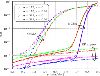
Figure 9: PLR comparison of optimized CSMA and B-CSA systems for different values of $n$ and $\epsilon$. Solid and the dashed lines show the performance of B-CSA and CSMA, respectively. The dash-dotted lines show the analytical PLR approximation obtained using (28).

It can also be seen from Fig. 9 that B-CSA significantly outperforms CSMA for medium to high channel loads. For example, for $\epsilon=0$, B-CSA achieves a PLR of $10^{-3}$ at channel loads $g=0.68$ and $g=0.73$ for $n=172$ and $n=315$, respectively. CSMA achieves the same reliability at $g=0.36$ and $g=0.32$ for $n=172$ and $n=315$, respectively, i.e., B-CSA can support approximately twice as many users as CSMA for this reliability. When erasures are present, the gains are even larger. For $\epsilon=0$, CSMA yields better PLR than B-CSA for low channel loads only ($g\lessapprox 0.3$). Moreover, CSMA shows better performance for heavily loaded networks ($g>0.84$). However, in this case both protocols provide a poor reliability (PLR of around $0.4$), which is unacceptable in VCs.

We remark that the high user mobility prohibits the use of acknowledgements in VCs, and thereby methods for mitigating the hidden terminal problem. Thus, the performance of CSMA will be severely affected by the hidden terminal problem in a real vehicular network. On the other hand, the problem of hidden terminals does not exist in B-CSA since collisions are used for decoding and no sensing is required.

VII Conclusion and Discussion

In this paper, we proposed a novel uncoordinated MAC protocol for a message exchange in the all-to-all broadcast scenario. Furthermore, we analyzed its performance over the PEC for finite frame length and proposed an accurate analytical approximation of the PLR performance in the EF region. The proposed analytical approximation can be used to optimize the degree distribution for CSA in the finite frame length regime. The analysis shows that B-CSA is robust to packet erasures and is able to support a much higher number of users that can communicate reliably than the state-of-the-art MAC protocol currently used for VCs.

In order to guarantee high reliability over the PEC, the physical (PHY) layer and the MAC protocol of a communication system should offer a certain level of time diversity. For protocols that do not exploit collisions, such as CSMA, increasing time diversity leads to channel congestion at low channel loads. Hence, exploiting collisions is inevitable for systems that require high reliability for high channel loads over the PEC. B-CSA is an elegant way of utilizing collisions. The obtained gains come at the expense of increased computation complexity that a system designer should be ready to pay if they wants to satisfy the stringent requirements of VCs.

References

- [1] N. Abramson, “Another alternative for computer communications,” in Proc. Fall Joint Computer Conf., 1970, pp. 281–285.
- [2] L. G. Roberts, “ALOHA packet system with and without slot and capture,” SIGCOMM Comput. Commun. Rev., vol. 5, no. 2, pp. 28–42, Apr. 1975.
- [3] G. Choudhury and S. Rappaport, “Diversity ALOHA-A random access scheme for satellite communications,” IEEE Trans. Commun., vol. 31, no. 3, pp. 450–457, Mar. 1983.
- [4] E. Casini, R. D. Gaudenzi, and O. Herrero, “Contention resolution diversity slotted ALOHA (CRDSA): An enhanced random access schemefor satellite access packet networks,” IEEE Trans. Wireless Commun., vol. 6, no. 6, pp. 1408–1419, Apr. 2007.
- [5] S. Gollakota and D. Katabi, “Zigzag decoding: Combating hidden terminals in wireless networks,” ACM SIGCOMM, pp. 159–170, 2008.
- [6] A. Tehrani, A. Dimakis, and M. Neely, “Sigsag: Iterative detection through soft message-passing,” IEEE J. Sel. Top. Sign. Proces., vol. 5, no. 8, pp. 1512–1523, Dec. 2011.
- [7] A. ParandehGheibi, J. K. Sundararajan, and M. Medard, “Collision helps - algebraic collision recovery for wireless erasure networks,” in Proc. IEEE Wirel. Network Coding Conf., Boston, MA, June 2010.
- [8] G. Liva, “Graph-based analysis and optimization of contention resolution diversity slotted ALOHA,” IEEE Trans. Commun., vol. 59, no. 2, pp. 477–487, Feb. 2011.
- [9] K. R. Narayanan and H. D. Pfister, “Iterative collision resolution for slotted ALOHA: an optimal uncoordinated transmission policy,” in Proc. Int. Symp. on Turbo Codes & Iterative Information Processing, Gothenburg, Sweden, Aug. 2012.
- [10] E. Paolini, G. Liva, and M. Chiani, “Coded slotted ALOHA: A graph-based method for uncoordinated multiple access,” IEEE Trans. Inf. Theory (to appear), 2016.
- [11] C. Stefanovic and P. Popovski, “ALOHA random access that operates as a rateless code,” IEEE Trans. Commun., vol. 61, no. 11, pp. 4653–4662, Nov. 2013.
- [12] R. Olfati-Saber, J. A. Fax, and R. M. Murray, “Consensus and cooperation in networked multi-agent systems,” Proc. of the IEEE, vol. 95, no. 1, pp. 215–233, Jan. 2007.
- [13] P. Popovski, “Ultra-reliable communication in 5G wireless systems,” in Proc. IEEE Int. Conf. 5G for Ubiquitous Connectivity, Levi, Finland, Nov. 2014.
- [14] N. A. Johansson, Y. Wang, E. Eriksson, and M. Hessler, “Radio access for ultra-reliable and low-latency 5G communications,” in Proc. IEEE Int. Conf. Commun., London, UK, June 2015.
- [15] G. Durisi, T. Koch, and P. Popovski, “Towards massive, ultra-reliable, and low-latency wireless communication with short packets,” Proc. of the IEEE (to appear), 2016.
- [16] C. Di, D. Proietti, I. E. Telatar, T. J. Richardson, and R. L. Urbanke, “Finite-length analysis of low-density parity-check codes on the binary erasure channel,” IEEE Trans. Inf. Theory, vol. 48, no. 6, pp. 1459–1473, June 2002.
- [17] C.-C. Wang, S. R. Kulkarni, and H. V. Poor, “Finding all small error-prone substructures in LDPC codes,” IEEE Trans. Inf. Theor., vol. 55, no. 5, pp. 1976–1999, May 2009.
- [18] E. Rosnes and O. Ytrehus, “An efficient algorithm to find all small-size stopping sets of low-density parity-check matrices,” IEEE Trans. Inf. Theor., vol. 55, no. 9, pp. 4167–4178, Sep. 2009.
- [19] A. Orlitsky, K. Viswanathan, and J. Zhang, “Stopping set distribution of LDPC code ensembles,” IEEE Trans. Inf. Theory, vol. 51, no. 3, pp. 929–953, Mar. 2005.
- [20] E. Paolini, “Finite length analysis of irregular repetition slotted ALOHA (IRSA) access protocols,” in Proc. IEEE Int. Conf. Commun. Workshop, London, UK, June 2015.
- [21] M. Ivanov, F. Brännström, A. Graell i Amat, and P. Popovski, “Error floor analysis of coded slotted ALOHA over packet erasure channels,” IEEE Commun. Lett., vol. 19, no. 3, pp. 419–422, Mar. 2015.
- [22] A. Guillén i Fàbregas, “Coding in the block-erasure channel,” IEEE Trans. Inf. Theory, vol. 52, no. 11, pp. 5116–5121, Nov. 2006.
- [23] A. Munari, M. Heindlmaier, G. Liva, and M. Berioli, “The throughput of slotted ALOHA with diversity,” in Proc. Allerton Conf. Commun., Control, and Computing, Monticello, IL, Oct. 2013.
- [24] O. D. R. Herrero and R. D. Gaudenzi, “Generalized analytical framework for the performance assessment of slotted random access protocols,” IEEE Trans. Wireless Commun., vol. 13, no. 2, pp. 809–821, Feb. 2014.
- [25] V. Lottici, A. D’Andrea, and U. Mengali, “Channel estimation for ultra-wideband communications,” IEEE J. Select. Areas Commun., vol. 20, no. 9, pp. 1638–1645, Dec. 2002.
- [26] B. Rimoldi and R. Urbanke, “A rate-splitting approach to the Gaussian multiple-access channel,” IEEE Trans. Inf. Theory, vol. 42, no. 2, pp. 364–375, Mar. 1996.
- [27] M. G. Luby, M. Mitzenmacher, M. A. Shokrollahi, and D. A. Spielman, “Analysis of low density codes and improved designs using irregular graphs,” in Proc. ACM Symp. on Theory of Computing, 1998.
- [28] T. J. Richardson and R. L. Urbanke, “The capacity of low-density parity-check codes under message-passing decoding,” IEEE Trans. Inf. Theory, vol. 47, no. 2, pp. 599–618, Feb. 2001.
- [29] J. A. Bondy and U. S. R. Murty, Graph Theory with Applications, 1st ed. North-Holland, 1976.
- [30] M. Ivanov, F. Brännström, A. Graell i Amat, and P. Popovski, “All-to-all broadcast for vehicular networks based on coded slotted ALOHA,” in Proc. IEEE Int. Conf. Commun. Workshop, London, UK, June 2015.
- [31] M. Luby, M. Mitzenmacher, and A. Shokrollahi, “Analysis of random processes via and-or tree evaluation,” in Proc. ACM-SIAM Symp. Discrete Algorithms, San Francisco, CA, Jan. 1998.
- [32] S. S. Skiena, The Algorithm Design Manual, 2nd ed. Springer, 2008.
- [33] S.-R. Lee, S.-D. Joo, and C.-W. Lee, “An enhanced dynamic framed slotted ALOHA algorithm for RFID tag identification,” in Proc. Int. Conf, on Mobile and Ubiquitous Systems: Networking and Services, San Diego, CA, July 2005.
- [34] W. E. Ryan and S. Lin, Channel codes: Classical and Modern, 1st ed. Cambridge University Press, 2009.
- [35] S. Boyd and L. Vandenberghe, Convex optimization, 1st ed. Cambridge University Press, 2009.
- [36] J. Lagarias, J. A. Reeds, M. H. Wright, and P. E. Wright, “Convergence properties of the Nelder-Mead simplex method in low dimensions,” SIAM Journal of Optimization, vol. 9, no. 1, pp. 112–147, 1998.
- [37] IEEE Std. 802.11-2012, “Part 11: Wireless LAN medium access control (MAC) and physical layer (PHY) specifications,” Tech. Rep., Mar. 2012.
- [38] ETSI EN 302 637-2: Draft V.0.0.5, “Intelligent transport systems (ITS); Vehicular communications; Basic set of applications; Part 2: Specification of cooperative awareness basic service,” Tech. Rep., June 2012.
- [39] K. Bilstrup, E. Uhlemann, E. Ström, and U. Bilstrup, “On the ability of the 802.11p MAC method and STDMA to support real-time vehicle-to-vehicle communication,” EURASIP J. on Wireless Commun. and Networking, vol. 2009, pp. 1–13, Apr. 2009.