Bootstrapping Empirical Processes of Cluster Functionals with Application to Extremograms

Abstract

In the extreme value analysis of time series, not only the tail behavior is of interest, but also the serial dependence plays a crucial role. Drees and Rootzén (2010) established limit theorems for a general class of empirical processes of so-called cluster functionals which can be used to analyse various aspects of the extreme value behavior of mixing time series. However, usually the limit distribution is too complex to enable a direct construction of confidence regions. Therefore, we suggest a multiplier block bootstrap analog to the empirical processes of cluster functionals. It is shown that under virtually the same conditions as used by Drees and Rootzén (2010), conditionally on the data, the bootstrap processes converge to the same limit distribution. These general results are applied to construct confidence regions for the empirical extremogram introduced by Davis and Mikosch (2009). In a simulation study, the confidence intervals constructed by our multiplier block bootstrap approach compare favorably to the stationary bootstrap proposed by Davis et al. (2012).

1 Introduction

Time series of observations in environmetrics, (financial) risk management and other fields often exhibit a non-negligible serial dependence between extremes. For example, stable areas of low (or high) pressure may lead to consecutive days of high precipitation (or high temperature). Likewise, large losses to a financial investment tend to occur in clusters.

The statistical analysis of the serial dependence structure between extreme observations is still a challenging task. Yet even if one is only interested in marginal parameters, like extreme quantiles, it is crucial to take into account the serial dependence when assessing the estimation error; see, e.g., Drees (2003) for a simulation study which demonstrates how misleading confidence intervals may be if the serial dependence is ignored.

In most applications, no parametric time series model for the extremal behavior suggests itself. Hence, one should resort to non-parametric procedures to avoid the risk of an unquantifiable, but potentially large modeling error. In this context, a general class of empirical processes that can capture a wide range of different aspects of the extremal behavior of time series prove a powerful tool.

To be more concrete, assume that a stationary time series $(X_{t})_{1\leq t\leq n}$ with values in $E=\mathbb{R}^{d}$ is observed, from which we construct $m_{n}:=\lfloor n/r_{n}\rfloor$ blocks

$$Y_{n,j}:=(X_{n,i})_{(j-1)r_{n}<i\leq jr_{n}},\quad 1\leq j\leq m_{n},$$ (1.1)

of “standardized extreme observations” $X_{n,i}$, $1\leq i\leq n$. A typical choice for univariate time series is

$$X_{n,i}:=(X_{i}-u_{n})^{+}/a_{n}:=a_{n}^{-1}(X_{i}-u_{n})1_{\{X_{i}>u_{n}\}}$$ (1.2)

for suitable normalizing constants $u_{n}\in\mathbb{R}$ and $a_{n}>0$. Later on, we will use a different notion of extreme observation in our application to the analysis of the extremogram, for a multivariate time series.

Denote by $E_{\cup}:=\bigcup_{l\in\mathbb{N}}E^{l}$ the set of vectors of arbitrary length with components in $E$, which is equipped with the $\sigma$-field $\mathbb{E}_{\cup}$ induced by the Borel-$\sigma$-fields on $E^{l}$, $l\in\mathbb{N}$. Let $\mathcal{F}$ be a family of so-called cluster functionals, i.e. functions $f:(E_{\cup},\mathbb{E}_{\cup})\to(\mathbb{R},\mathbb{B})$ such that $f(0)=0$ and $f(y_{1},\ldots,y_{l})=f(0,\ldots,0,y_{1},\ldots,y_{l},0,\ldots,0)$ for all $(y_{1},\ldots,y_{l})\in E_{\cup}$ where the numbers of coordinates equal to 0 in the beginning and in the end of the argument on the right-hand side can be arbitrary. Thus the value of the cluster functional depends only on the core of the argument, which is the smallest subvector of consecutive coordinates that contains all non-zero values (resp. it equals 0 if the argument only consists of zeros). Then, the pertaining empirical process of cluster functionals is defined by

$$Z_{n}(f):=\frac{1}{\sqrt{nv_{n}}}\sum_{j=1}^{m_{n}}\big{(}f(Y_{n,j})-Ef(Y_{n,j})\big{)},\quad f\in\mathcal{F},$$ (1.3)

with $v_{n}:=P\{X_{n,1}\neq 0\}$. Drees and Rootzén (2010) established sufficient conditions for $Z_{n}$ to converge to a Gaussian process in the space $\ell^{\infty}(\mathcal{F})$ of bounded functions on $\mathcal{F}$. The following theorem summarizes their main results; the conditions are recalled in the appendix.

1.1 Theorem 

1. If the conditions (B1), (B2) and (C1)–(C3) are fulfilled, the finite-dimensional marginal distributions (fidis) of the empirical process $Z_{n}$ converge to the pertaining fidis of a Gaussian process $Z$ with covariance function $c$ (defined in (C3)).

2. Under the conditions (B1), (B2) and (D1)–(D4) the empirical process $Z_{n}$ is asymptotically tight in $\ell^{\infty}(\mathcal{F})$. If, in addition, the conditions (C1)–(C3) are met, then $Z_{n}$ weakly converges to $Z$.

3. If the assumptions (B1), (B2), (D1), (D2’), (D3) and (D5) are satisfied and, in addition, (D6) (or the more restrictive condition (D6’)) holds, then $Z_{n}$ is asymptotically equicontinuous. Hence, $Z_{n}$ weakly converges to $Z$ in $\ell^{\infty}(\mathcal{F})$ if also the conditions (C1)–(C3) hold.

$\Box$

For certain types of families $\mathcal{F}$ of cluster functionals, Drees and Rootzén (2010) also gave sets of conditions that are sufficient for $(Z_{n}(f))_{f\in\mathcal{F}}$ to converge and easier to verify than the abstract conditions listed in the appendix.

We will demonstrate their usefulness by improving on limit results on an empirical version of the so-called extremogram introduced by Davis and Mikosch (2009) in the framework of time series with regularly varying marginals. To be more precise, assume that $(X_{t})_{t\in\mathbb{Z}}$ is a stationary $\mathbb{R}^{d}$-valued time series such that for all $h\in\mathbb{N}$ the vector $(X_{0},X_{h})\in\mathbb{R}^{2d}$ is regularly varying. Recall that a random vector $W\in\mathbb{R}^{l}$ is regularly varying if there exists a non-null measure $\nu$ on $\mathbb{R}^{l}\setminus\{0\}$ such that

$$\frac{P\{W\in xB\}}{P\{\|W\|>x\}}\;\longrightarrow\;\nu(B)<\infty$$

for all $\nu$-continuity sets $B\in\mathbb{B}^{l}$ that are bounded away from the origin 0. Note that, while this definition of regular variation does not depend on the choice of the norm $\|\cdot\|$, the specific form of the limiting measure $\nu$ does. In any case, the limiting measure is homogeneous of order $-\alpha$ for some $\alpha>0$, the so-called index of regular variation.

Then, with $F_{\|X\|}^{\leftarrow}$ denoting the quantile function of $\|X_{0}\|$ and $a_{n}:=F_{\|X\|}^{\leftarrow}(1-1/n)\to\infty$, to each lag $h\in\mathbb{N}$ there exists a measure $\nu_{(0,h)}$ on $\mathbb{R}^{2d}\setminus\{0\}$ such that

$$nP\{a_{n}^{-1}(X_{0},X_{h})\in B\}\;\longrightarrow\;\nu_{(0,h)}(B)$$ (1.4)

for all $\nu_{(0,h)}$-continuity sets $B\in\mathbb{B}^{2d}$ bounded away from the origin. In particular, for all $A,B\in\mathbb{B}^{d}$ bounded away from 0 such that $\nu_{h}(\partial(A\times B))=0=\nu_{h}(\partial(A\times\mathbb{R}^{d}))$ and $\nu_{h}(A\times\mathbb{R}^{d})>0$ one has

$$P(X_{h}\in a_{n}B\mid X_{0}\in a_{n}A)=\frac{P\{a_{n}^{-1}(X_{0},X_{h})\in A\times B\}}{P\{a_{n}^{-1}X_{0}\in A\}}\;\longrightarrow\;\frac{\nu_{(0,h)}(A\times B)}{\nu_{(0,h)}(A\times R^{d})}=:\rho_{A,B}(h).$$

Davis and Mikosch (2009) called $\rho_{A,B}$ (as a function of $h$) the extremogram of $(X_{t})_{t\in\mathbb{Z}}$ (pertaining to $A,B$). It is worth mentioning that the extremogram is closely related to the concept of tail processes introduced by Basrak and Segers (2008).

Based on the observations $X_{1},\ldots,X_{n}$, they proposed the following empirical counterpart as an estimator of $\rho_{A,B}(h)$:

$$\hat{\rho}_{A,B}(h):=\frac{\sum_{i=1}^{n-h}{\boldsymbol{1}_{\textstyle\{X_{i}\in a_{k}A,X_{i+h}\in a_{k}B\}}}}{\sum_{i=1}^{n}{\boldsymbol{1}_{\textstyle\{X_{i}\in a_{k}A\}}}}.$$ (1.5)

Here $k=k_{n}$ is a sequence that tends to $\infty$ at a slower rate than $n$ so that $a_{k}\to\infty$ at a slower rate than $a_{n}$, and thus the number of extreme observations used for estimation tends to $\infty$. Under suitable conditions, $(\hat{\rho}_{A,B}(h))_{h\in\{0,\ldots,h_{0}\}}$ is asymptotically normal (see Davis and Mikosch, 2009, Corollary 3.4).

This result has two serious drawbacks. First, usually, the normalizing constants $a_{k}$ are unknown and must hence be replaced with an empirical counterpart, like, e.g., the $\lfloor n/k\rfloor+1$ largest observed norm:

$$\hat{a}_{k}:=\hat{a}_{k,n}:=\|X\|_{n-\lfloor n/k\rfloor:n}.$$ (1.6)

It is not obvious whether this modification influences the asymptotic behavior of the empirical extremogram.

Secondly, the extremogram for a fixed pair of sets $A$ and $B$ conveys limited information on the extremal dependence structure, in particular in a multivariate setting, i.e. if $d>1$. To get a fuller picture, one should consider the extremogram for a whole family of sets simultaneously. For example, in the case $d=1$, Drees et al. (2015) considered rays $(-\infty,-x)$ and $(x,\infty)$ for all $x>0$ simultaneously. However, the techniques used by Davis and Mikosch (2009) are not applicable to infinite families of sets.

We will show that both problems can be neatly solved using the theory of empirical processes of cluster functionals. Indeed, if the families of sets $A$ and $B$ are suitably chosen and the bias of $\hat{\rho}_{A,B}(h)$ is asymptotically negligible, then the asymptotic normality of the empirical extremogram with estimated normalizing sequence $\hat{a}_{k}$ follows immediately.

If one wants to construct confidence regions using this limit theorem, then estimators of the limiting covariance structure are needed. Since the direct estimation does not look promising, Davis et al. (2012) proposed to use a so-called stationary bootstrap instead. Here we follow a somewhat different approach. First, in the general setting considered by Drees and Rootzén (2010), it is shown that the convergence of a multiplier block bootstrap version of the empirical process of cluster functional conditionally given the data follows under the same conditions as the convergence of $Z_{n}$ itself. From this powerful result it is easily concluded that a multiplier block bootstrap version can be used to construct confidence regions for the extremogram.

Though in the present paper we focus on the extremogram as one possible measure for the extremal dependence structure of the time series, the same approach using empirical processes of cluster functionals can be used in a much wider context. For example, Drees (2011) analyzed block estimators of the so-called extremal index of absolutely regular time series using empirical processes of cluster functionals and suggested a bias corrected version thereof.

The paper is organized as follows. In Section 2 we introduce multiplier block bootstrap versions of the empirical process $Z_{n}$. Moreover, we give sufficient conditions under which, in probability conditional on the data, this bootstrap processes weakly converge to the same limiting process as $Z_{n}$. In Section 3, it is demonstrated that the theory developed by Drees and Rootzén (2010) yields limit theorems for the empirical extremogram with estimated normalizing sequence uniformly over suitable families of sets. In the same setup, a bootstrap result easily follows from the general theory developed in Section 2. The results of a small simulation study are reported in Section 3. All proofs are postponed to Section 5.

Throughout the paper, we will use the notation $x^{(k)}$ for the vector $(x_{1},\ldots,x_{k})$ made up by the first $k$ components in the vector $x$, if $x$ has at least $k$ components, and otherwise $x^{(k)}=x$. The maximum norm of a vector $x\in\mathbb{R}^{l}$ for some $l\in\mathbb{N}$ is denoted by $\|x\|$. We omit indices of random variables to denote a generic random variable with the same distribution; for example, $\xi$ is a generic random variable with the same distribution as $\xi_{j}$ and $Y_{n}$ is a generic random vector with the same distribution as $Y_{n,j}$.

2 Multiplier processes

In what follows, $(X_{n,i})_{1\leq i\leq n,n\in\mathbb{N}}$ is a row-wise stationary triangular scheme of $E=\mathbb{R}^{d}$-valued random vectors. Usually these vectors are derived from some fixed stationary time series $(X_{t})_{t\in\mathbb{Z}}$ by a transformation which depends on the stage $n$ and which sets all but the “extreme” observations to 0 in such a way that the probability that a transformed observation is non-zero tends to 0 as $n\to\infty$. For univariate time series, often definition (1.2) is used. In our application to the empirical extremogram instead we define

$$X_{n,i}^{(h,\tilde{h})}:=a_{k}^{-1}\big{(}X_{i}{\boldsymbol{1}_{\textstyle\{X_{i}\not\in(-\infty,a_{k}x_{*})^{d}\}}},X_{i+h}{\boldsymbol{1}_{\textstyle\{X_{i+h}\not\in(-\infty,a_{k}x_{*})^{d}\}}},X_{i+\tilde{h}}{\boldsymbol{1}_{\textstyle\{X_{i+\tilde{h}}\not\in(-\infty,a_{k}x_{*})^{d}\}}}\big{)}$$ (2.1)

for some $x_{*}>0$ and $h,\tilde{h}\in\mathbb{N}_{0}$.

According to Theorem 1.1, under suitable conditions, the empirical process $Z_{n}$ of cluster functionals converge to a Gaussian process $Z$ with covariance function $c$, which is defined in (C3) as the limit of the covariance function of the cluster functionals applied to a block $Y_{n}$ of $r_{n}$ consecutive “standardized extremes” $X_{n,i}$. One may try to estimate this covariance function by an empirical covariance, but since most of the blocks $Y_{n,j}$ defined in (1.1) equal 0, a bootstrap approach seems more promising.

Because the processes are defined via functionals applied to whole blocks $Y_{n,j}$ of “standardized extremes”, it suggests itself to use some block bootstrap. More precisely, we consider the following two versions of multiplier block bootstrap processes:

$$Z_{n,\xi}(f) := \frac{1}{\sqrt{nv_{n}}}\sum_{j=1}^{m_{n}}\xi_{j}\big{(}f(Y_{n,j})-Ef(Y_{n,j})\big{)},$$ (2.2)

$$Z_{n,\xi}^{*}(f) := \frac{1}{\sqrt{nv_{n}}}\sum_{j=1}^{m_{n}}\xi_{j}\big{(}f(Y_{n,j})-\overline{f(Y_{n})}\big{)},\quad f\in\mathcal{F},$$ (2.3)

where $\overline{f(Y_{n})}:=m_{n}^{-1}\sum_{j=1}^{m_{n}}f(Y_{n,j})$ and $\xi_{j},j\in\mathbb{N}$, are i.i.d. random variables with $E(\xi_{j})=0$ and $Var(\xi_{j})=1$ independent of $(X_{n,i})_{1\leq i\leq n,n\in\mathbb{N}}$. Note that in the definition of the multiplier process $Z_{n,\xi}$ expectations $Ef(Y_{n})$ are used which are usually unknown to the statistician. Hence, in some applications, it may be useful to replace them with the estimators $\overline{f(Y_{n})}$, which leads to the bootstrap processes $Z_{n,\xi}^{*}$.

Our main goal is to prove weak convergence of $Z_{n,\xi}$ and $Z_{n,\xi}^{*}$ to $Z$ in probability, conditionally on the data. To this end, as usual, we metrize weak convergence in $\ell^{\infty}(\mathcal{F})$ using the bounded Lipschitz metric on the space of probability measures on $\ell^{\infty}(\mathcal{F})$. That is, for two probability measures $Q_{1}$ and $Q_{2}$ we define

$$d_{BL(\ell^{\infty}(\mathcal{F}))}(Q_{1},Q_{2}):=\sup_{g\in BL_{1}(\ell^{\infty}(\mathcal{F}))}\Big{|}\int g\,dQ_{1}-\int g\,dQ_{2}\Big{|},$$

where

$$BL_{1}(\ell^{\infty}(\mathcal{F})) := \big{\{}g:\ell^{\infty}(\mathcal{F})\to\mathbb{R}\mid\|g\|_{\infty}:=\sup_{z\in\ell^{\infty}(\mathcal{F})}|g(z)|\leq 1,$$

$$\hskip 14.22636pt|g(z_{1})-g(z_{2})|\leq\|z_{1}-z_{2}\|_{\mathcal{F}}:=\sup_{f\in\mathcal{F}}|z_{1}(f)-z_{2}(f)|\text{ for all }z_{1},z_{2}\in\ell^{\infty}(\mathcal{F})\big{\}}.$$

Likewise, for the convergence of the fidis, we use the distance

$$d_{BL(\mathbb{R}^{l})}(Q_{1},Q_{2}):=\sup_{g\in BL_{1}(\mathbb{R}^{l})}\Big{|}\int g\,dQ_{1}-\int g\,dQ_{2}\Big{|},$$

between two probability measures $Q_{1}$ and $Q_{2}$ on $\mathbb{R}^{l}$, where

$$BL_{1}(\mathbb{R}^{l}):=\big{\{}g:\mathbb{R}^{l}\to\mathbb{R}\mid\sup_{v\in\mathbb{R}^{l}}|g(v)|\leq 1,|g(v_{1})-g(v_{2})|\leq\|v_{1}-v_{2}\|\text{ for all }v_{1},v_{2}\in\mathbb{R}^{l}\big{\}}.$$

By $E_{\xi}$ (resp. $E_{\xi}^{*}$) we denote the (outer) expectation with respect to $(\xi_{j})_{j\in\mathbb{N}}$, i.e.$E_{\xi}\big{(}f(\xi_{1},\ldots,\xi_{m_{n}},X_{n,1},\ldots,X_{n,n})\big{)}=E\big{(}f(\xi_{1},\ldots,\xi_{m_{n}},X_{n,1},\ldots,X_{n,n})\mid X_{n,1},\ldots,X_{n,n}\big{)}$ is the expectation of the function conditionally on the observations. Likewise, we denote by $P_{\xi}$ the probability measure w.r.t. $(\xi_{j})_{j\in\mathbb{N}}$. (Cf. Kosorok, 2003, for a precise definition using a special construction of probability spaces.)

Our first result shows that the asymptotic behavior of the fidis of $Z_{n,\xi}$, conditionally on the data, is the same as the (unconditional) behavior of the fidis of $Z_{n}$.

2.1 Theorem 

Under the conditions (B1), (B2) and (C1)–(C3) one has for all $f_{1},\ldots,f_{l}\in\mathcal{F}$

$$\sup_{g\in BL_{1}(\mathbb{R}^{l})}\Big{|}E_{\xi}g\big{(}(Z_{n,\xi}(f_{k}))_{1\leq k\leq l}\big{)}-Eg\big{(}(Z(f_{k}))_{1\leq k\leq l}\big{)}\Big{|}\;\longrightarrow\;0$$ (2.4)

in probability. $\Box$

Since the supremum in (2.4) is bounded by 2, it readily follows that

$$\sup_{g\in BL_{1}(\mathbb{R}^{l})}\Big{|}Eg\big{(}(Z_{n,\xi}(f_{k}))_{1\leq k\leq l}\big{)}-Eg\big{(}(Z(f_{k}))_{1\leq k\leq l}\big{)}\Big{|}$$

$$\leq E\sup_{g\in BL_{1}(\mathbb{R}^{l})}\Big{|}E_{\xi}g\big{(}(Z_{n,\xi}(f_{k}))_{1\leq k\leq l}\big{)}-Eg\big{(}(Z(f_{k}))_{1\leq k\leq l}\big{)}\Big{|}\;\longrightarrow\;0,$$

that is, the (unconditional) weak convergence of the fidis of $Z_{n,\xi}=(Z_{n,\xi}(f))_{f\in\mathcal{F}}$ to the corresponding fidis of $Z$.

Following the ideas developed by Kosorok (2003), the following result establishes the asymptotic tightness of $Z_{n,\xi}$ under a bracketing entropy condition, and thus also the weak convergence of $Z_{n,\xi}$ under the same conditions as the convergence of the original empirical process in Theorem 1.1(ii).

2.2 Proposition 

Suppose that the conditions (B1), (B2), (D1), (D3) and (D4) hold and

1. (D2) holds and $\xi$ is bounded, or

2. (D2’) holds and $E^{*}(F^{2}(Y_{n}))=O(r_{n}v_{n})$.

Then $Z_{n,\xi}$ is asymptotically tight in $l^{\infty}(\mathcal{F})$. Hence it converges to $Z$ if, in addition, the conditions (C1)–(C3) are met. $\Box$

Now a modification of the arguments given in the proof of Theorem 2 of Kosorok (2003) yields the desired convergence result for the multiplier process conditionally on the data.

2.3 Theorem 

If condition (D3) and convergence (2.4) hold and $Z_{n,\xi}$ weakly converges to $Z$, then

$$\sup_{g\in BL_{1}(\ell^{\infty}(\mathcal{F}))}\big{|}E_{\xi}g(Z_{n,\xi})-Eg(Z)\big{|}\;\longrightarrow\;0$$ (2.5)

in outer probability. $\Box$

A combination of this result with Theorem 2.1 and Proposition 2.2 leads to

2.4 Corollary 

If the conditions (B1), (B2), (C1)-(C3) and (D1)-(D4) are satisfied and $\xi$ is bounded, then convergence (2.5) holds. $\Box$

According to Theorem 2.3, under (D3) the weak convergence of the multiplier process $Z_{n,\xi}$ to $Z$ conditionally on the data follows from the weak convergence of the fidis conditionally on the data and the (unconditional) convergence of $Z_{n,\xi}$ to $Z$. The latter assertion may also be derived by establishing the asymptotic equicontinuity of $Z_{n,\xi}$ using a metric entropy condition (instead of verifying tightness using a bracketing entropy condition as in Proposition 2.2).

2.5 Proposition 

Suppose that the conditions (B1), (B2), (D1), (D2’), (D3) and
(D5’)    For all $\delta>0,n\in\mathbb{N},(e_{i})_{1\leq i\leq\lfloor m_{n}/2\rfloor}\in\{-1,0,1\}^{\lfloor m_{n}/2\rfloor}$ and $k\in\{1,2\}$ the map $\sup_{f,g\in\mathcal{F},\rho(f,g)<\delta}$ $\sum_{j=1}^{\lfloor m_{n}/2\rfloor}e_{j}\big{(}\xi_{j}(f(Y_{n,j}^{*})-g(Y_{n,j}^{*}))\big{)}^{k}$ is measurable
are fulfilled and

1. (D6) holds and $\xi$ is bounded, or

2. (D6’) holds.

Then $Z_{n,\xi}$ is asymptotically equicontinuous. Hence, it converges to $Z$ if, in addition, the conditions (C1)–(C3) are met. $\Box$

Using Theorem 2.3 and Corollary 2.6.12 of van der Vaart and Wellner (1996), we obtain as an immediate consequence

2.6 Corollary 

If the conditions (B1), (B2), (C1)-(C3), (D1), (D2’), (D3) and (D5’) are met, if $F$ is measurable with $E(F^{2}(Y_{n}))=O(r_{n}v_{n})$ and $\mathcal{F}$ is a VC-hull class, then convergence (2.5) holds. $\Box$

To sum up, we have shown that, roughly under the same conditions as used in Theorem 1.1, the multiplier process $Z_{n,\xi}$ shows the same asymptotic behavior conditionally on the data as the empirical process $Z_{n}$ unconditionally. The following result gives conditions under which the convergence of $Z_{n,\xi}$ implies the convergence of the bootstrap process $Z_{n,\xi}^{*}$ conditionally on the data.

2.7 Corollary 

If convergence (2.4) of the fidis of $Z_{n,\xi}$ holds conditionally on the data, condition (D3) is satisfied and $Z_{n}\to Z$ and $Z_{n,\xi}\to Z$ weakly, then

$$E_{\xi}\sup_{f\in\mathcal{F}}|Z_{n,\xi}^{*}(f)-Z_{n,\xi}(f)|\;\longrightarrow\;0$$ (2.6)

in outer probability, $Z_{n,\xi}^{*}\to Z$ weakly and

$$\sup_{g\in BL_{1}(\ell^{\infty}(\mathcal{F}))}\big{|}E_{\xi}g(Z_{n,\xi}^{*})-Eg(Z)\big{|}\;\longrightarrow\;0$$ (2.7)

in outer probability. In particular, these assertions hold under the conditions of Corollary 2.4 and under the assumptions of Corollary 2.6. $\Box$

2.8 Remark 

Note that also the normalizing factor $(nv_{n})^{-1/2}$ in the definition of $Z_{n,\xi}^{*}$ may be unknown. In most applications of multiplier processes, though, this is not problematic, because this factor is not needed to construct confidence regions. Nevertheless, it is noteworthy that assertion (2.7) remains valid if $v_{n}$ is replaced with some estimator $\hat{v}_{n}$ that is consistent in the sense that $\hat{v}_{n}/v_{n}\to 1$ in probability. $\Box$

For specific types of cluster functionals, Drees and Rootzén (2010) gave simpler sufficient conditions for the convergence of the corresponding empirical process which carry over to the multiplier processes considered here. In the next section we will use the conditions of Corollary 3.6 of that paper, which deals with so-called generalized tail array sums, i.e. empirical processes with functionals of the form $f_{\phi}(y_{1},\ldots,y_{r})=\sum_{i=1}^{r}\phi(y_{i})$ for functions $\phi:(E,\mathbb{E})\to(\mathbb{R},\mathbb{B})$ such that $\phi(0)=0$.

3 Processes of Extremograms

In this section we employ the general theory to analyze the asymptotic behavior of the empirical extremogram $\hat{\rho}_{n,A,B}$, a version with empirical normalization and a bootstrap version thereof, uniformly over suitable families of sets $A$ and $B$ and over lags $h\in\{0,\ldots,h_{0}\}$ for some fixed $h_{0}\in\mathbb{N}$. Throughout this section we are only interested in the behavior for vectors with at least one large component. We thus consider families $\mathcal{C}$ of pairs of measurable subsets of $\mathbb{R}^{d}$ such that

$$x_{*}:=\inf_{(A,B)\in\mathcal{C}}\inf_{x\in A}\max_{1\leq j\leq d}x_{j}>0,$$

i.e. $A\subset\mathbb{R}^{d}\setminus(-\infty,x_{*})^{d}$ for all $(A,B)\in\mathcal{C}$. However, the results below can be generalized to families of sets that are uniformly bounded away from 0 so that $\inf_{(A,B)\in\mathcal{C}}\inf_{x\in A}\max_{1\leq j\leq d}|x_{j}|>0$. For the sake of notational simplicity, we assume that $n+h_{0}$ (instead of $n$) $\mathbb{R}^{d}$-valued random vectors $X_{1},\ldots,X_{n+h_{0}}$ are observed.

3.1 Remark 

To keep the presentation simple, we will assume that $X_{0}$ is regularly varying on the full cone $\mathbb{R}^{d}\setminus\{0\}$ with a limiting measure $\nu_{0}$ which is not concentrated on $(-\infty,0]^{d}$; see Theorem 3.2 below. This assumption could be weakened to the regular variation on the cone $\mathbb{R}^{d}\setminus(-\infty,0]^{d}$ defined in the spirit of Das et al. (2013), i.e. there exists a normalizing sequence $\tilde{a}_{n}>0$ and a measure $\tilde{\nu}_{0}$ such that

$$nP\{X_{0}/\tilde{a}_{n}\in B\}\;\longrightarrow\;\tilde{\nu}_{0}(B)$$

for all $\tilde{\nu}_{0}$-continuity sets $B\in\mathbb{B}$ bounded away from $(-\infty,0]^{d}$, where the limit has to be finite. Here one may choose $\tilde{a}_{n}$ as the $(1-1/n)$-quantile of $\max_{1\leq j\leq d}X_{0,j}$. Under the slightly more restrictive assumption used in the results below, one has

$$\frac{P\{\max_{1\leq j\leq d}X_{0,j}>u\}}{P\{\|X_{0}\|>u\}}\;\longrightarrow\;\nu_{0}\big{(}\mathbb{R}^{d}\setminus(-\infty,1]^{d}\big{)}$$

as $u\to\infty$, and hence $\tilde{a}_{n}\sim a_{n}\big{(}\nu_{0}\big{(}\mathbb{R}^{d}\setminus(-\infty,1]^{d}\big{)}\big{)}^{1/\alpha}$ and $\tilde{\nu}_{0}=\nu_{0}/\nu_{0}\big{(}\mathbb{R}^{d}\setminus(-\infty,1]^{d}\big{)}$, where $-\alpha$ is the degree of homogeneity of $\nu_{0}$, i.e. $\nu_{0}(\lambda B)=\lambda^{-\alpha}\nu_{0}(B)$. $\Box$

For some intermediate sequence $k=k_{n}$ (i.e. $k_{n}\to\infty$, $k_{n}/n\to 0$), we define the empirical extremogram to the sets $A$ and $B$ and lag $h$ as

$$\hat{\rho}_{n,A,B}(h):=\frac{\textstyle\sum_{i=1}^{n}1_{A\times B}(X_{i}/a_{k},X_{i+h}/a_{k})}{\textstyle\sum_{i=1}^{n}1_{A}(X_{i}/a_{k})}.$$

Note that this is a slight modification of the definition given by Davis and Mikosch (2009) in that we do not use the maximal number of summands in the denominator. However, it is easily seen that all results given below carry over to the original definition.

The uniform asymptotic behavior of the empirical extremogram will easily follow from that of the stochastic process

$$\tilde{Z}_{n}(h,A,B) := \frac{1}{\sqrt{nv_{n}}}\sum_{i=1}^{n}\Big{(}1_{A\times B}(X_{i}/a_{k},X_{i+h}/a_{k})-P\{X_{i}\in a_{k}A,X_{i+h}\in a_{k}B\}\Big{)},$$

$h\in\{0,\ldots,h_{0}\},(A,B)\in\mathcal{C},$ with

$$v_{n}:=P\{X_{0}\not\in(-\infty,a_{k}x_{*})^{d}\}.$$

This process, in turn, can be analyzed using the theory for empirical processes of cluster functionals developed by Drees and Rootzén (2010). In order to use conditions on the joint distribution of the $X_{t}$ as weak as possible, it is useful to consider such processes indexed by $(A,B)\in\mathcal{C}$ and just two lags $h,\tilde{h}\in\{0,\ldots,h_{0}\}$. Let

$$\tilde{X}_{n,i} := \frac{X_{i}}{a_{k}}1_{\mathbb{R}^{d}\setminus(-\infty,x_{*})^{d}}\Big{(}\frac{X_{i}}{a_{k}}\Big{)},\quad 1\leq i\leq n+h_{0},$$

$$X_{n,i}^{(h,\tilde{h})} := (\tilde{X}_{n,i},\tilde{X}_{n,i+h},\tilde{X}_{n,i+\tilde{h}}),\quad 1\leq i\leq n,$$

$$Y_{n,j}^{(h,\tilde{h})} := (X_{n,i}^{(h,\tilde{h})})_{(j-1)r_{n}<i\leq jr_{n}},\quad 1\leq j\leq m_{n},$$

$$v_{n}^{(h,\tilde{h})} := P\{X_{n,i}^{(h,\tilde{h})}\neq 0\}=P\{(X_{0},X_{h},X_{\tilde{h}})\not\in(-\infty,x_{*})^{3d}\},$$

$$\mathcal{D} := \{A\times B\times\mathbb{R}^{d},A\times\mathbb{R}^{d}\times B\mid(A,B)\in\mathcal{C}\},$$

$$f_{D}(y_{1},\ldots,y_{r}) := \sum_{i=1}^{r}1_{D}(y_{i}),\quad y_{i}\in\mathbb{R}^{3d},\quad D\in\mathcal{D},$$

$$\mathcal{F} := \{f_{D}\mid D\in\mathcal{D}\},\quad\text{and}$$

$$Z_{n}^{(h,\tilde{h})}(f_{D}) := \frac{1}{\sqrt{nv_{n}^{(h,\tilde{h})}}}\sum_{j=1}^{m_{n}}\big{(}f_{D}(Y_{n,j}^{(h,\tilde{h})})-Ef_{D}(Y_{n,j}^{(h,\tilde{h})})\big{)}$$

$$= \frac{1}{\sqrt{nv_{n}^{(h,\tilde{h})}}}\sum_{i=1}^{m_{n}r_{n}}\big{(}1_{D}(X_{n,i}^{(h,\tilde{h})})-P\{X_{n,i}^{(h,\tilde{h})}\in D\}\big{)},\quad D\in\mathcal{D}.$$

Note that, for $n=m_{n}r_{n}$, we have $\tilde{Z}_{n}(h,A,B)=(v_{n}^{(h,\tilde{h})}/v_{n})^{1/2}Z_{n}^{(h,\tilde{h})}(f_{A\times B\times\mathbb{R}^{d}})$ and $\tilde{Z}_{n}(\tilde{h},A,B)=(v_{n}^{(h,\tilde{h})}/v_{n})^{1/2}Z_{n}^{(h,\tilde{h})}(f_{A\times\mathbb{R}^{d}\times B})$; under the conditions of Theorem 3.2 the difference between these processes is asymptotically negligible even if $m_{n}r_{n}<n$.

Using Corollary 3.6 of Drees and Rootzén (2010) and Drees and Rootzén (2015), we obtain the following set of sufficient conditions for the convergence of $\tilde{Z}_{n}$.

3.2 Theorem 

Suppose that all four-dimensional marginal distributions of the stationary time series $(X_{t})_{t\in\mathbb{N}_{0}}$ are regularly varying, i.e. for all index vectors $I\in\mathbb{N}_{0}^{l}$ of dimension $l\leq 4$ there exists a measure $\nu_{I}$ such that

$$nP\{a_{n}^{-1}X_{I}\in B\}\;\longrightarrow\,\nu_{I}(B)<\infty$$ (3.1)

for all Borel sets $B$ bounded away from $0\in\mathbb{R}^{ld}$, and that $\nu_{0}(\mathbb{R}^{d}\setminus(-\infty,x^{*})^{d})>0$. In addition, assume that the conditions (B1), (B2) and ($\widetilde{\text{B3}}$) are fulfilled, and $r_{n}=o(\sqrt{nv_{n}})$. Finally, assume that there exists a bounded semi-metric $\bar{\varrho}$ on $\mathcal{C}$ such that $\mathcal{C}$ is totally bounded w.r.t. $\bar{\varrho}$, and a function $u:(0,\infty)\to(0,\infty)$ such that $\lim_{t\downarrow 0}u(t)=0$ and

$$E\Big{(}\sum_{i=1}^{r_{n}}1_{(A\times B)\Delta(\tilde{A}\times\tilde{B})}(X_{i}/a_{k},X_{i+h}/a_{k})\Big{)}^{2}\leq u\big{(}\bar{\varrho}\big{(}(A,B),(\tilde{A},\tilde{B})\big{)}\big{)}r_{n}v_{n}$$ (3.2)

for all $(A,B),(\tilde{A},\tilde{B})\in\mathcal{C}$, $h\in\{0,\ldots,h_{0}\}$, and that the conditions (D5) and (D6) hold for $\varrho\big{(}f_{D},f_{\tilde{D}}\big{)}:=\bar{\varrho}\big{(}(A,B),(\tilde{A},\tilde{B})\big{)}$ if $D=A\times B\times\mathbb{R}^{d}$, $\tilde{D}=\tilde{A}\times\tilde{B}\times\mathbb{R}^{d}$, or $D=A\times\mathbb{R}^{d}\times B$, $\tilde{D}=\tilde{A}\times\mathbb{R}^{d}\times\tilde{B}$, and $\varrho\big{(}f_{D},f_{\tilde{D}}\big{)}:=L$ else for some sufficiently large constant $L>1$. (Here $C_{1}\Delta C_{2}$ denotes the symmetric difference of the two sets $C_{1}$ and $C_{2}$.)

Then $\tilde{Z}_{n}$ converges weakly to a Gaussian process $\tilde{Z}$ with covariance function

$$\tilde{c}\big{(}(h,A,B),(\tilde{h},\tilde{A},\tilde{B})\big{)}:=\sum_{i=-\infty}^{\infty}\frac{\nu_{(0,h,i,i+\tilde{h})}(A\times B\times\tilde{A}\times\tilde{B})}{\nu_{0}\big{(}\mathbb{R}^{d}\setminus(-\infty,x_{*})^{d}\big{)}}<\infty.$$

$\Box$

Observe that in (3.1) necessarily the following consistency condition holds: for vectors $I_{0}=(i_{j})_{1\leq j\leq l}$ and $I=(i_{j})_{1\leq j\leq 4}$ of indices and $\nu_{I_{0}}$-continuity sets $A\in\mathbb{B}^{ld}$ bounded away from the origin one has $\nu_{I_{0}}(A)=\nu_{I}(A\times\mathbb{R}^{(4-l)d})$.

Usually the moment condition (3.2) and the entropy condition (D6) are most difficult to verify. The proof of Theorem 3.2 shows that the process $\tilde{Z}_{n}$ indexed by $\tilde{\mathcal{F}}:=\{(h,A,B)\mid h\in\{0,\ldots,h_{0}\},(A,B)\in\mathcal{C}\}$ is asymptotically tight if and only if the empirical processes $Z_{n}^{(h,\tilde{h})}$ indexed by $\{f_{A\times B\times\mathbb{R}^{d}}\mid(A,B)\in\mathcal{C}\}$ resp. $\{f_{A\times\mathbb{R}^{d}\times B}\mid(A,B)\in\mathcal{C}\}$ are asymptotically tight for all $h,\tilde{h}\in\{0,\ldots,h_{0}\}$. Thus we may replace condition (D6) by the assumption that these families are VC-subgraph class of functions, which in turn is equivalent to the assumption that

$$\bar{\mathcal{F}}:=\{\bar{f}_{A\times B}\mid(A,B)\in\mathcal{C}\}\quad\text{with}\quad\bar{f}_{D}(y_{1},\ldots,y_{r}):=\sum_{i=1}^{r}1_{D}(y_{i})\;\;\text{for}\;\;y_{i}\in\mathbb{R}^{2d},1\leq i\leq r,$$ (3.3)

is a VC-subgraph class of functions. Likewise, one may divide the family $\mathcal{C}$ into a finite number of subfamilies $\mathcal{C}_{j}$ and check that $\bar{\mathcal{F}}_{j}:=\{\bar{f}_{A\times B}\mid(A,B)\in\mathcal{C}_{j}\}$ is a VC-subgraph class of functions.

For applications to the asymptotic analysis of empirical extremograms, we shall consider families $\mathcal{C}$ such that for $(A,B)\in\mathcal{C}$ also $(A,\mathbb{R}^{d})$ belongs to $\mathcal{C}$. The following simple example exhibits another closedness property of $\mathcal{C}$ which is important to prove convergence of the empirical extremogram with estimated normalizing constant.

3.3 Example 

Fix some $\lambda_{0}>0$ and measurable sets $A_{0},B_{0}\subset\mathbb{R}^{d}$ bounded away from 0 such that $x\in A_{0}$ implies $\lambda x\in A_{0}$ for all $\lambda>1$ and likewise for $x\in B_{0}$. (In particular, one may choose a set $A_{0}\subset[0,\infty)^{d}\setminus[0,1]^{d}$ such that $x\in A_{0}$ and $y\geq x$ imply $y\in A_{0}$.) Then, for $\mathcal{C}_{1}:=\{\lambda(A_{0},B_{0})\mid\lambda>\lambda_{0}\}$, the family $\bar{\mathcal{F}}_{1}$ is a VC-subgraph class of functions. To see this, note that $\bar{f}_{\lambda(A\times B)}\leq f_{\tilde{\lambda}(A\times B)}$ if $\lambda>\tilde{\lambda}$, i.e. the functions are linearly ordered. Hence no set of size 2 can be shattered by the subgraphs of $\bar{\mathcal{F}}_{1}$. Likewise, the family $\bar{\mathcal{F}}_{2}$ pertaining to $\mathcal{C}_{2}:=\{\lambda(A_{0},\mathbb{R}^{d})\mid\lambda>\lambda_{0}\}$ is a VC-subgraph class of functions.

Condition (3.2) can be reformulated as follows. There exists a semi-metric $\tilde{\varrho}$ on $[\lambda_{0},\infty)$ such that $[\lambda_{0},\infty)$ is totally bounded w.r.t. $\tilde{\varrho}$ and $E\big{(}\sum_{i=1}^{r_{n}}1_{(\lambda(A_{0}\times B_{0}))\setminus(\tilde{\lambda}(A_{0}\times B_{0}))}(X_{i}/a_{k},X_{i+h}/a_{k})\big{)}^{2}\leq u(\tilde{\varrho}(\lambda,\tilde{\lambda}))r_{n}v_{n}$ and $E\big{(}\sum_{i=1}^{r_{n}}1_{(\lambda A_{0})\setminus(\tilde{\lambda}A_{0})}(X_{i}/a_{k})\big{)}^{2}\leq u(\tilde{\varrho}(\lambda,\tilde{\lambda}))r_{n}v_{n}$ hold for all $\lambda_{0}<\lambda<\tilde{\lambda}$ and all $n\in\mathbb{N}$. $\Box$

The families of sets $A$ and $B$ most widely discussed in the literature are sets of upper right orthants $(x,\infty)$ and complements $\mathbb{R}^{d}\setminus(-\infty,x]$ of lower left orthants.

3.4 Example 

Consider the family $\mathcal{C}_{1}:=\big{\{}\big{(}(x_{A},\infty),(x_{B},\infty)\big{)}\mid x_{A},x_{B}\not\in(-\infty,x_{*}]^{d}\big{\}}$ of pairs of upper right orthants bounded away from the origin. Then condition (D6) holds for $\mathcal{C}:=\mathcal{C}_{1}\cup\big{\{}\big{(}(x_{A},\infty),\mathbb{R}^{d}\big{)}|x_{A}\not\in(-\infty,x_{*}]^{d}\big{\}}$ if condition (B1) is satisfied and

$$E\Big{(}\sum_{i=1}^{r_{n}}1_{\{X_{i}\not\in(-\infty,a_{k}x_{*})^{d}\}}\Big{)}^{2+\delta}=O(r_{n}v_{n}),$$ (3.4)

for some $\delta>0$. (see Section 5).

By the same arguments one can show that condition (D6) is fulfilled for the family $\mathcal{C}:=\big{\{}\big{(}\mathbb{R}^{d}\setminus(-\infty,x_{A}],\mathbb{R}^{d}\setminus(-\infty,x_{B}]\big{)},\big{(}\mathbb{R}^{d}\setminus(-\infty,x_{A}],\mathbb{R}^{d}\big{)}\mid x_{A},x_{B}\in(x_{*},\infty)^{d}\big{\}}$. $\Box$

From Theorem 3.2 one may easily conclude the uniform asymptotic normality of the empirical extremogram centered at the pre-asymptotic extremogram

$$\rho_{t,A,B}(h):=P(X_{h}/t\in B\mid X_{0}/t\in A).$$

3.5 Corollary 

Suppose that the conditions of Theorem 3.2 are met, that $(A,\mathbb{R}^{d})\in\mathcal{C}$ for all $(A,B)\in\mathcal{C}$ and $\inf_{(A,B)\in\mathcal{C}}\nu_{0}(A)>0$, and that $\sup_{h\in\{0,\ldots,h_{0}\},(A,B)\in\mathcal{C}}|\rho_{a_{k},A,B}(h)-\rho_{A,B}(h)|\to 0$. Then

$$\sqrt{nv_{n}}\Big{(}\hat{\rho}_{n,A,B}(h)-\rho_{a_{k},A,B}(h)\Big{)}_{h\in\{0,\ldots,h_{0}\},(A,B)\in\mathcal{C}}$$ (3.5)

$$\to \Big{(}\frac{\nu_{0}\big{(}\mathbb{R}^{d}\setminus(-\infty,x_{*})^{d}\big{)}}{\nu_{0}(A)}\big{(}\tilde{Z}(h,A,B)-\rho_{A,B}(h)\tilde{Z}(h,A,\mathbb{R}^{d})\big{)}\Big{)}_{h\in\{0,\ldots,h_{0}\},(A,B)\in\mathcal{C}}$$

$$=: (R(h,A,B))_{h\in\{0,\ldots,h_{0}\},(A,B)\in\mathcal{C}}$$

weakly. Hence if, in addition,

$$\sup_{h\in\{0,\ldots,h_{0}\},(A,B)\in\mathcal{C}}\sqrt{\frac{n}{k}}|\rho_{a_{k},A,B}(h)-\rho_{A,B}(h)|\to 0,$$ (3.6)

then

$$\sqrt{nv_{n}}\Big{(}\hat{\rho}_{n,A,B}(h)-\rho_{A,B}(h)\Big{)}_{h\in\{0,\ldots,h_{0}\},(A,B)\in\mathcal{C}}\to(R(h,A,B))_{h\in\{0,\ldots,h_{0}\},(A,B)\in\mathcal{C}}$$

weakly. $\Box$

We have already mentioned in the introduction that the empirical extremogram $\hat{\rho}_{n,A,B}(h)$ is not a valid estimator if the normalizing constants $a_{k}$ are unknown. In this case we replace them by some estimator $\hat{a}_{k}$ which is consistent in the sense that $\hat{a}_{k}/a_{k}\to 1$ in probability. Noting that

$$\hat{\hat{\rho}}_{n,A,B}(h):=\frac{\textstyle\sum_{i=1}^{n}1_{A\times B}(X_{i}/\hat{a}_{k},X_{i+h}/\hat{a}_{k})}{\textstyle\sum_{i=1}^{n}1_{A}(X_{i}/\hat{a}_{k})}=\hat{\rho}_{n,(\hat{a}_{k}/a_{k})A,(\hat{a}_{k}/a_{k})B}(h),$$

the asymptotic normality of $\hat{\hat{\rho}}_{n,A,B}(h)$ is an easy consequence of Corollary 3.5, provided that $\rho_{t,A,B}(h)$ is a sufficiently regular function of $t$.

3.6 Corollary 

Assume that the conditions of Corollary 3.5 (except (3.6)) are fulfilled and, in addition, $\hat{a}_{k}/a_{k}\to 1$ in probability, that $(A,B)\in\mathcal{C}$ implies $(\lambda A,\lambda B)\in\mathcal{C}$ for all $\lambda$ in a neighborhood of 1 and that $\sup_{(A,B)\in\mathcal{C}}\bar{\varrho}\big{(}(A,B),(\lambda A,\lambda B)\big{)}\to 0$ as $\lambda\to 1$. Then

$$\sqrt{nv_{n}}\Big{(}\hat{\hat{\rho}}_{n,A,B}(h)-\rho_{\hat{a}_{k},A,B}(h)\Big{)}_{h\in\{0,\ldots,h_{0}\},(A,B)\in\mathcal{C}}\to(R(h,A,B))_{h\in\{0,\ldots,h_{0}\},(A,B)\in\mathcal{C}}$$

weakly. Hence, if the following second order condition holds

$$\rho_{t,A,B}(h)=\rho_{A,B}(h)+\Phi_{h}(t)\Psi_{h}(A,B)+o(\Phi_{h}(t))$$ (3.7)

uniformly for $h\in\{0,\ldots,h_{0}\}$, $(A,B)\in\mathcal{C}$, and some extended regularly varying function $\Phi_{h}$ (see Bingham et al., 1987, Section 2.0) satisfying $\Phi_{h}(t)\to 0$ as $t\to\infty$ and some functions $\Psi_{h}$ such that $\sup_{(A,B)\in\mathcal{C}}|\Psi_{h}(A,B)|<\infty$, then

$$\sqrt{nv_{n}}\Big{(}\hat{\hat{\rho}}_{n,A,B}(h)-\rho_{a_{k},A,B}(h)\Big{)}_{h\in\{0,\ldots,h_{0}\},(A,B)\in\mathcal{C}}\to(R(h,A,B))_{h\in\{0,\ldots,h_{0}\},(A,B)\in\mathcal{C}}$$

weakly, provided $\Phi_{h}(a_{k})=O((k/n)^{1/2})$. If $\Phi_{h}(a_{k})=o((k/n)^{1/2})$, then this convergence holds with $\rho_{A,B}(h)$ instead of $\rho_{a_{k},A,B}(h)$. $\Box$

3.7 Remark 

1. If $(X_{0},X_{h})$ satisfies the second order condition

   $$a^{\leftarrow}(t)P\{(X_{0},X_{h})/t\in A\times B\}=\nu_{(0,h)}(A\times B)+\Phi_{h}(t)\tilde{\Psi}_{h}(A\times B)+o(\Phi_{h}(t))$$ (3.8)

   uniformly for all $(A,B)\in\mathcal{C}$ with $\sup_{(A,B)\in\mathcal{C}}|\tilde{\Psi}_{h}(A\times B)|<\infty$, then under the conditions of Corollary 3.6 direct calculations show that $\rho_{t,A,B}(h)=P\{(X_{0},X_{h})/t\in A\times B\}/P\{(X_{0},X_{h})/t\in A\times\mathbb{R}^{d}\}$ satisfies condition (3.7) with $\Psi_{h}(A,B)=\big{(}\tilde{\Psi}_{h}(A\times B)-\rho_{A,B}(h)\tilde{\Psi}_{h}(A\times\mathbb{R}^{d})\big{)}/\nu_{0}(A).$

2. If the conditions of Theorem 3.2 hold when (3.2) is replaced with

   $$E\Big{(}\sum_{i=1}^{r_{n}}1_{[-y,y]^{d}\setminus[-x,x]^{d}}(X_{i}/a_{k})\Big{)}^{2}\leq u(y-x)r_{n}v_{n}$$

   for all $1-\delta\leq x<y\leq 1+\delta$, $n\in\mathbb{N}$, and some function $u$ satisfying $u(t)\to 0$ as $t\downarrow 0$, then the same arguments as used in the proof of Theorem 3.2 show that

   $$\frac{1}{\sqrt{n/k}}\sum_{i=1}^{n}\Big{(}{\boldsymbol{1}_{\textstyle\{\|X_{i}\|/a_{k}>x\}}}-P\{\|X_{i}\|/a_{k}>x\}\Big{)}=\sqrt{kv_{n}}\tilde{Z}_{n}(0,\mathbb{R}^{d}\setminus[-x,x]^{d},\mathbb{R}^{d}),\quad x\in[1-\delta,1+\delta],$$

   converges weakly to a continuous Gaussian process. From $P\{\|X_{0}\|/a_{k}>x\}\sim x^{-\alpha}/k$ and

   $$\frac{\|X\|_{n-\lfloor n/k\rfloor:n}}{a_{k}}$$

   $$= \inf\Big{\{}x\,\Big{|}\,\sum_{i=1}^{n}{\boldsymbol{1}_{\textstyle\{\|X_{i}\|/a_{k}>x\}}}\leq\lfloor n/k\rfloor\Big{\}}$$

   $$= \inf\Big{\{}x\,\Big{|}\,\sqrt{kv_{n}}\tilde{Z}_{n}(0,\mathbb{R}^{d}\setminus[-x,x]^{d},\mathbb{R}^{d})\leq(k/n)^{1/2}\big{(}\lfloor n/k\rfloor-nP\{\|X_{0}\|/a_{k}>x\}\big{)}\Big{\}},$$

   one can easily conclude that $\|X\|_{n-\lfloor n/k\rfloor:n}/a_{k}\to 1$ in probability, i.e. $\|X\|_{n-\lfloor n/k\rfloor:n}$ is consistent for $a_{k}$.

   Indeed, a refined analysis shows that under the second order condition (3.8) one even has $\|X\|_{n-\lfloor n/k\rfloor:n}/a_{k}-1=O_{P}((k/n)^{1/2})$ if $\Phi(a_{k})=O_{P}((k/n)^{1/2})$.

$\Box$

As the distribution of the limit process arising in Corollary 3.6 is difficult to estimate, we use the bootstrap approach discussed in Section 2 to approximate the distribution of the empirical extremogram. Let

$$\hat{\rho}^{*}_{n,A,B}(h) := \frac{\sum_{j=1}^{m_{n}}(1+\xi_{j})\sum_{i=1}^{r_{n}}1_{A\times B}\big{(}a_{k}^{-1}(X_{(j-1)r_{n}+i},X_{(j-1)r_{n}+i+h})\big{)}}{\sum_{j=1}^{m_{n}}(1+\xi_{j})\sum_{i=1}^{r_{n}}1_{A}\big{(}a_{k}^{-1}X_{(j-1)r_{n}+i}\big{)}}$$

$$\hat{\hat{\rho}}^{*}_{n,A,B}(h) := \frac{\sum_{j=1}^{m_{n}}(1+\xi_{j})\sum_{i=1}^{r_{n}}1_{A\times B}\big{(}\hat{a}_{k}^{-1}(X_{(j-1)r_{n}+i},X_{(j-1)r_{n}+i+h})\big{)}}{\sum_{j=1}^{m_{n}}(1+\xi_{j})\sum_{i=1}^{r_{n}}1_{A}\big{(}\hat{a}_{k}^{-1}X_{(j-1)r_{n}+i}\big{)}}$$

$$= \hat{\rho}^{*}_{n,(\hat{a}_{k}/a_{k})A,(\hat{a}_{k}/a_{k})B}(h)$$

$$R_{n,\xi}(h,A,B) := \sqrt{nv_{n}}\big{(}\hat{\rho}^{*}_{n,A,B}(h)-\hat{\rho}_{n,A,B}(h)\big{)}$$

$$\hat{R}_{n,\xi}(h,A,B) := \sqrt{nv_{n}}\big{(}\hat{\hat{\rho}}^{*}_{n,A,B}(h)-\hat{\hat{\rho}}_{n,A,B}(h)\big{)}=R_{n,\xi}(h,(\hat{a}_{k}/a_{k})A,(\hat{a}_{k}/a_{k})B).$$

3.8 Theorem 

Suppose that all conditions of Corollary 3.6 are fulfilled and that $\xi_{j}$, $j\in\mathbb{N}$, are i.i.d. random variables with $E(\xi_{1})=0$ and $Var(\xi_{1})=1$ independent of $(X_{t})_{t\in\mathbb{N}_{0}}$. Then,

$$\sup_{g\in BL_{1}(\ell^{\infty}(\{0,\ldots,h_{0}\}\times\mathcal{C}))}\big{|}E_{\xi}g(R_{n,\xi})-Eg(R)\big{|} \to 0$$ (3.9)

$$\sup_{g\in BL_{1}(\ell^{\infty}(\{0,\ldots,h_{0}\}\times\mathcal{C}))}\big{|}E_{\xi}g(\hat{R}_{n,\xi})-Eg(R)\big{|} \to 0\quad\text{in probability.}$$ (3.10)

$\Box$

Let $\tilde{\mathcal{F}}:=\{0,\ldots,h_{0}\}\times\mathcal{C}$. In view of Theorem 3.8, approximate confidence regions for the extremogram $(\rho_{A,B}(h))_{(h,A,B)\in\tilde{\mathcal{F}}}$ can be obtained from Monte Carlo simulations of $\hat{\hat{\rho}}^{*}_{n,A,B}(h)$. To this end, suppose $\mathcal{D}$ is a family of subsets of $\ell^{\infty}(\tilde{\mathcal{F}})$ such that $\sup_{D\in\mathcal{D}}P\{R\in U_{\varepsilon}(\partial D)\}\to 0$ as $\varepsilon\downarrow 0$, where $U_{\varepsilon}(A)$ denotes the open $\varepsilon$-neighborhood of a set $A$ w.r.t. the supremum norm $\|\cdot\|_{\tilde{\mathcal{F}}}$ on $\ell^{\infty}(\tilde{\mathcal{F}})$. Then all indicator functions $1_{D}$, $D\in\mathcal{D}$, can be uniformly well approximated from above and from below by functions of the form $g_{\varepsilon,A}:=(1-d_{A}/\varepsilon)^{+}$ with $d_{A}(z):=\inf_{\tilde{z}\in A}\|z-\tilde{z}\|$. Since the functions $\varepsilon g_{\varepsilon,A}$ belong to $BL_{1}(\ell^{\infty}(\tilde{\mathcal{F}}))$, it is easily seen that (3.9) and (3.10) imply $\sup_{D\in\mathcal{D}}\big{|}P_{\xi}\{R_{n,\xi}\in D\}-P\{R\in D\}\big{|}\to 0$ and $\sup_{D\in\mathcal{D}}\big{|}P_{\xi}\{\hat{R}_{n,\xi}\in D\}-P\{R\in D\}\big{|}\to 0$ as $n\to\infty$, respectively.

In particular, if for sufficiently large $n\in\mathbb{N}$, $D_{\alpha}$ is a subset of $\ell^{\infty}(\tilde{\mathcal{F}})$ such that

$$P_{\xi}\big{\{}(\hat{\hat{\rho}}^{*}_{n,A,B}(h)-\hat{\hat{\rho}}_{n,A,B}(h))_{(h,A,B)\in\tilde{\mathcal{F}}}\in D_{\alpha}\big{\}}=\alpha,$$ (3.11)

then under the conditions of Corollary 3.6 with $\Phi(a_{k})=o((k/n)^{1/2})$, for sufficiently large $n$, we have

$$P\big{\{}(\hat{\hat{\rho}}_{n,A,B}(h)-\rho_{A,B}(h))_{(h,A,B)\in\tilde{\mathcal{F}}}\in D_{\alpha}\big{\}}\approx\alpha.$$ (3.12)

To find such a set (or rather an approximation to it), one may simulate $B$ independent realizations $(\hat{\hat{\rho}}^{*(b)}_{n,A,B}(h))_{(h,A,B)\in\tilde{\mathcal{F}}}$, $1\leq b\leq B$, of the bootstrap version of the empirical extremogram. For some fixed set $D\subset\ell^{\infty}(\tilde{\mathcal{F}})$ let $D_{\alpha}:=\lambda_{\alpha}D$ with $\lambda_{\alpha}$ denoting the smallest $\lambda\geq 0$ such that

$$\frac{1}{B}\sum_{b=1}^{B}1_{\textstyle\big{\{}\big{(}\hat{\hat{\rho}}^{*(b)}_{n,A,B}(h)-\hat{\hat{\rho}}_{n,A,B}(h)\big{)}_{(h,A,B)\in\tilde{\mathcal{F}}}\in\lambda D\big{\}}}\geq\alpha.$$

Here $D$ ought to be star-shaped, i.e. $z\in D$ implies $\lambda z\in D$ for all $\lambda\in[0,1]$. The shape of $D$ determines the emphasis which is laid on particular features of the extremogram. See Section 4 for an example.

4 Finite sample performance of bootstrapped extremograms

In this section we investigate the finite sample performance of confidence intervals which are constructed using the multiplier block bootstrap approach, the stationary bootstrap proposed by Davis et al. (2012) and a modified version of the latter.

Davis et al. (2012) suggested to construct bootstrap samples from an observed time series $(X_{t})_{1\leq t\leq n}$ as follows. Let $K_{i}$, $1\leq i\leq n$, be iid random variables uniformly distributed on $\{1,\ldots,n\}$, and $L_{i}$, $1\leq i\leq n$, iid random block lengths with a geometric distribution with expectation $r$, independent of $(K_{i})_{1\leq i\leq n}$. Define $S_{j}:=\sum_{i=1}^{j}L_{i}$, $0\leq j\leq n$, $N:=\min\{j|S_{j}\geq n\}$, and $L_{j}^{*}:=L_{j}$ for $1\leq j<N$ and $L_{N}^{*}:=n-S_{N-1}$. For $i\in\{S_{j-1}+1,S_{j-1}+2,\ldots,S_{j}\}$, $1\leq j\leq N$, let $X_{i}^{*}:=X_{K_{j}-1+i-S_{j-1}}$, where $X_{t}$ for $t>n$ is interpreted as $X_{(t\text{ mod }(n-1))+1}$. This means that blocks of length $L_{j}$ starting from the observation at $K_{j}$ are glued together until one obtains a new time series $(X_{t}^{*})_{1\leq t\leq n}$ of length $n$; in this process one repeats the original time series after the last observation as often as necessary. Now denote by $\hat{\rho}^{(*DMC)}_{n,A,B}(h)$ the bootstrap estimator of $\rho_{A,B}(h)$ calculated from $(X_{t}^{*})_{1\leq t\leq n}$. Davis et al. (2012) proved that under suitable conditions, conditionally on the data, the limit distribution of $\hat{\rho}^{(*DMC)}_{n,A,B}(h)-\hat{\rho}_{n,A,B}(h)$ is the same as the one of $\hat{\rho}_{n,A,B}(h)-\rho_{a_{k},A,B}(h)$, so that bootstrap confidence intervals can be constructed.

One disadvantage of this approach is that for indices $i$ near the end of a block such that $i\leq S_{j}<i+h$ for some $1\leq j<N$ the indicator ${\boldsymbol{1}_{\textstyle\{X^{*}_{i}\in a_{k}A,X^{*}_{i+h}\in a_{k}B\}}}$ has a completely different behavior than ${\boldsymbol{1}_{\textstyle\{X_{i}\in a_{k}A,X_{i+h}\in a_{k}B\}}}$, because $(X^{*}_{i},X^{*}_{i+h})$ does not correspond to a pair of observations with lag $h$ in the original time series.

To overcome this drawback, we suggest the following modification of the stationary bootstrap estimator. For simplicity, we assume that the time series has been observed at $n+h$ time points (in other words, we redefine $n$). Then we define

$$\hat{\rho}_{n,A,B}^{(*stat)}(h):=\frac{\sum_{j=1}^{N}\sum_{i=1}^{L_{j}^{*}}{\boldsymbol{1}_{\textstyle\{X_{K_{j}-1+i}\in a_{k}A,X_{K_{j}-1+i+h}\in a_{k}B\}}}}{\sum_{j=1}^{N}\sum_{i=1}^{L_{j}^{*}}{\boldsymbol{1}_{\textstyle\{X_{K_{j}-1+i}\in a_{k}A\}}}}$$

which has the same asymptotic behavior as $\hat{\rho}^{(*DMC)}_{n,A,B}(h)$, but only observations are compared which are lagged by $h$. In essence, this mean that we apply the stationary bootstrap technique to the bivariate time series $(X_{t},X_{t+h})_{1\leq t\leq n}$.

In addition to these two version of stationary bootstrap estimators, we consider the multiplier bootstrap. Here we have drawn multipliers $\xi_{j}$ from a Student $t$-distribution with 5 degrees of freedom and scale parameter such that $Var(\xi_{j})=1$. However, this particular choice is not crucial as in further simulations we have obtained a similar performance of the multiplier block bootstrap for other distributions which are symmetric about 1 with an unbounded support (e.g., for normally distributed multiplier).

Here we report the results for three different models:

1. a GARCH model $X_{t}=\sigma_{t}\varepsilon_{t}$, $\sigma_{t}^{2}=\alpha_{0}+\alpha_{1}X_{t-1}^{2}+\beta_{1}\sigma_{t-1}^{2}$ with $\alpha_{0}=10^{-4},\alpha_{1}=0.08,\beta_{1}=0.9$ and $t$-distributed innovations $\varepsilon_{t}$ with 8 degrees of freedom, independent of $\sigma_{t}$

2. an autoregressive model of order 1: $X_{t}=\varphi X_{t-1}+\varepsilon_{t}$ with $\varphi=0.8$ and symmetrized Fréchet distribution of the innovations, i.e., $P\{\varepsilon_{t}>x\}=P\{\varepsilon_{t}<-x\}=(1-\exp(-x^{-3}))/2$ for all $x>0$

3. a moving average time series of order 3, namely $X_{t}=\varepsilon_{t}+0.5\varepsilon_{t-1}+0.8\varepsilon_{t-2}$ with $\varepsilon_{t}$ as in (ii).

For each model we simulated $10\,000$ time series of length $n=2000$.

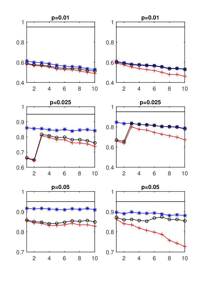
Figure 1: Empirical coverage probability of confidence intervals (4.1) for $\rho_{a_{k},(1,\infty),(1,\infty)}(h)$ as a function of $h$, constructed using multiplier block bootstrap (blue $*$), stationary bootstrap suggested by Davis et al. (red $+$) and the modification thereof (black $\circ$) with (average) block length $r=100$ (left) and $r=20$ (right) for the $t$-GARCH model (i), different thresholds $a_{k}$ with exceedance probability $p$ are used in the three rows; the nominal coverage probability 0.95 is indicated by the horizontal line.

We consider the extremogram for $A=B=(1,\infty)$, i.e., $\lim_{u\to\infty}P(X_{h}>u|X_{0}>u)$, which is often also called tail dependence coefficient, and lags $1\leq h\leq 10$. As normalizing constants $a_{k}$ (thresholds) we have chosen the $(1-p)$-quantile of the stationary distribution for $p\in\{0.01,0.025,0.05\}$ which have been estimated by the corresponding empirical quantiles. The true pre-asymptotic extremograms have been determined by simulation (based on 1000 time series of length $10^{7}$). Analytic expression for the (asymptotic) extremograms are known for the linear models (ii) and (iii) (see e.g., Meinguet and Segers, 2010, Example 9.2). For the GARCH model, they were determined using a simulation algorithm suggested by Ehlert et al. (2015).

In each simulation we have drawn $b=1000$ bootstrap replicas according to each of the three bootstrap procedures. If, for fixed $h$, the upper and lower empirical $\alpha/2$-quantile of the resulting $b$ bootstrap estimates of the extremogram are denoted by $u_{b}$ and $l_{b}$ then, according to (3.11) and (3.12),

$$\big{[}2\hat{\rho}_{n,A,B}(h)-u_{b},2\hat{\rho}_{n,A,B}(h)-l_{b}\big{]}\cap[0,1]$$ (4.1)

is a confidence interval for the (pre-asymptotic) extremogram with nominal coverage probability $1-\alpha$.

We first discuss the results for the $t$-GARCH model in detail, before we show the results for the linear time series in abbreviated form. For this model, Figure 1 shows the empirical coverage probabilities of all three bootstrap procedures as a function of $h$ for the pre-asymptotic extremogram. The three rows correspond to the three thresholds with ascending exceedance probabilities. The left column shows the results for (average) block length $r=100$, the right column for $r=20$. For all bootstrap procedures, the actual coverage probabilities are much smaller than the nominal value 0.95 if the threshold is chosen too high. For the estimator based on the largest 5% of the observations and blocks of length $r=100$, the coverage probability of the multiplier block bootstrap is reasonably close to the nominal size while both versions of the stationary bootstrap have a considerably lower coverage probability. In all simulations, the multiplier block bootstrap yields the highest coverage probability, while the stationary bootstrap proposed by Davis et al. (2012) performs worst. Moreover, in most cases the performance is better for larger block sizes. In particular, the stationary bootstrap proposed by Davis et al. is sensitive to too small a block size, as was to be expected from the above discussion.

The main reason for the disappointing performance for high thresholds is that then for very few or even none time instants both $X_{t}$ and $X_{t+h}$ exceed the threshold. If there are no joint exceedances in the original time series (leading to an estimate 0 for the extremogram) then also the bootstrap estimate equals 0 if one uses the multiplier block bootstrap or the modified stationary bootstrap (and it equals 0 for the original stationary bootstrap with very high probability). Hence the confidence intervals do not cover the true value if this is not exactly equal to 0, which is neither the case for the pre-asymptotic nor the asymptotic extremogram, leading to a high non-coverage probability. Indeed, for $p=0.01$, Figure 2 shows that if one considers only those simulations when the estimated extremogram does not equal 0, then the empirical coverage probability is rather close to the nominal value.

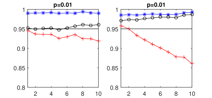
Figure 2: Empirical coverage probability of confidence intervals (4.1) for the pre-asymptotic extremogram $\rho_{a_{k},(1,\infty),(1,\infty)}(h)$ as a function of $h$, constructed using multiplier block bootstrap (blue $*$), stationary bootstrap suggested by Davis et al. (red $+$) and the modification thereof (black $\circ$) with (average) block length $r=100$ (left) and $r=20$ (right) for the $t$-GARCH model (i), based only on those simulations in which for some $t$ both $X_{t}$ and $X_{t+h}$ exceed the threshold $a_{k}$.

To overcome this weakness, we suggest to estimate the error distribution using a bootstrap based on a lower threshold if one wants to construct confidence intervals for the pre-asymptotic extremogram for a high threshold (or even the extremogram). Denote by $\hat{\rho}_{n,p}$ the empirical extremogram based on the exceedances over the threshold with exceedance probability $p$, and by $\hat{\rho}_{n,p}^{*}$ some bootstrap version thereof. Then, according to Theorem 3.8, conditional on the data, for $0<p_{1}<p_{2}$, the bootstrap error $\hat{\rho}_{n,p_{1}}^{*}-\hat{\rho}_{n,p_{1}}$ has approximately the same distribution as $(p_{2}/p_{1})^{1/2}\big{(}\hat{\rho}_{n,p_{2}}^{*}-\hat{\rho}_{n,p_{2}})$. So if $u_{b}$ and $l_{b}$ denote the empirical bootstrap quantiles as defined above, calculated from the bootstrap for the threshold with the higher exceedance probability $p_{2}$, then

$$\Big{[}\hat{\rho}_{n,p_{1}}-(p_{2}/p_{1})^{1/2}\big{(}u_{b}-\hat{\rho}_{n,p_{2}}),\hat{\rho}_{n,p_{1}}-(p_{2}/p_{1})^{1/2}\big{(}l_{b}-\hat{\rho}_{n,p_{2}})\Big{]}\cap[0,1]$$ (4.2)

is a confidence interval with nominal coverage probability $1-\alpha$.

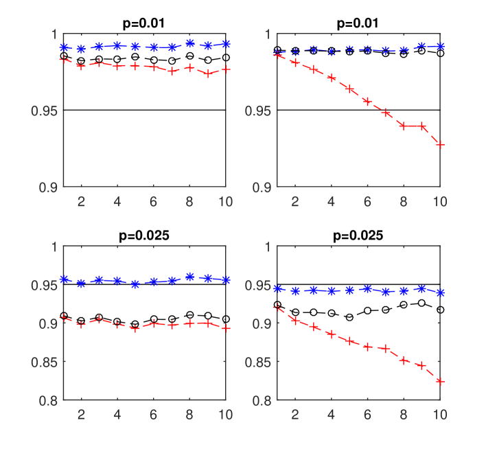
Figure 3: Empirical coverage probability of confidence intervals (4.2) for $\rho_{a_{k},(1,\infty),(1,\infty)}(h)$ as a function of $h$, constructed using multiplier block bootstrap (blue $*$), stationary bootstrap suggested by Davis et al. (red $+$) and the modification thereof (black $\circ$) with (average) block length $r=100$ (left) and $r=20$ (right) for the $t$-GARCH model (i).

Figure 3 displays the empirical coverage probabilities of this confidence interval for the pre-asymptotic extremogram, $p_{1}\in\{0.01,0.025\}$ and $p_{2}=0.05$, which are now much closer to the nominal size 0.95. (Indeed, for $p_{1}=0.01$ the new confidence intervals are a bit too conservative.) As for small $p_{1}$ the pre-asymptotic extremograms are closer to the limit extremograms, for these thresholds one may also be interested in the coverage probability for the latter, which are shown in Figure 4. The confidence intervals based on the threshold with exceedance probabilities $p_{1}=0.01$ are still a bit conservative, while for $p_{1}=0.025$, when the bias is larger and the confidence intervals more narrow, the actual coverage probabilities are too low.

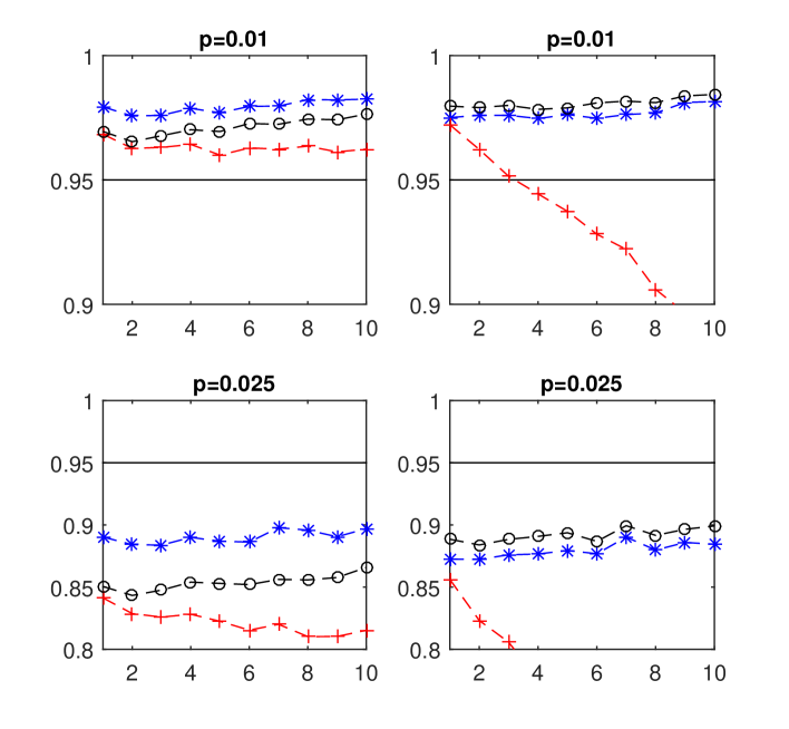
Figure 4: Empirical coverage probability of confidence intervals (4.2) (4.1) for the exremogram $\rho_{(1,\infty),(1,\infty)}(h)$ as a function of $h$, constructed using multiplier block bootstrap (blue $*$), stationary bootstrap suggested by Davis et al. (red $+$) and the modification thereof (black $\circ$) with (average) block length $r=100$ (left) and $r=20$ (right) for the $t$-GARCH model (i).

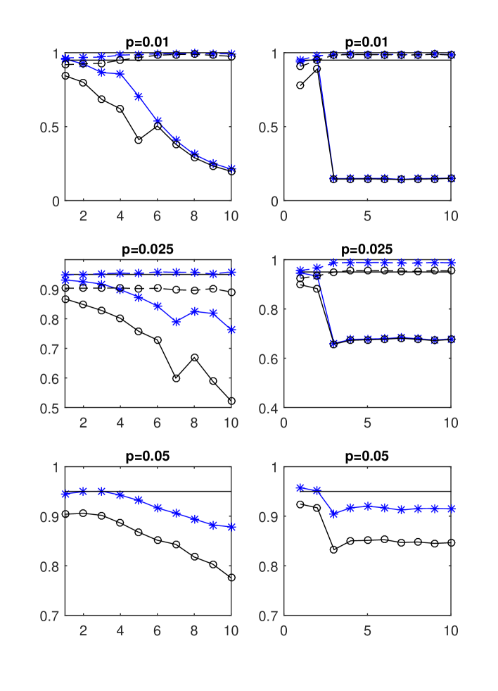
Figure 5: Empirical coverage probability of confidence intervals (4.1) (solid lines) and (4.2) (dashed lines) constructed using multiplier block bootstrap (blue $*$) and modified stationary bootstrap (black $\circ$) with block length $r=100$ for the AR(1) model (ii) (left) and MA(3) model (iii) (right) and different thresholds with exceedance probability $p$; the nominal coverage probability 0.95 is indicated by the horizontal line.

Finally, we briefly discuss the linear time series models. As overall the conclusions are similar, we present just the most important findings for block size $r=100$. Figure 5 shows the coverage probabilities for the autoregressive model (ii) in the left column and for the moving average (iii) in the right column, both for the confidence intervals (4.1) (solid lines) and (4.2) (dashed lines). In order to not overload the plot, the results for the original stationary bootstrap (which again performed worst) are not shown. Again the multiplier block bootstrap gives the highest coverage probabilities, which are nevertheless not satisfactory if one uses the direct bootstrap interval (4.1) for a high threshold for the extremogram at lags not close to 0. This is particularly true, if the true value is small (e.g., for large lags in the autoregressive model). In these cases, it helps a lot to borrow strength from the bootstrap for a lower threshold as in (4.2).

5 Proofs

Proof of Theorem 2.1.  We combine ideas from the proofs of Theorem 2.3 of Drees and Rootzén (2010) and of Theorem 2 by Kosorok (2003). Denote by $Y_{n,j}^{*}$, $1\leq j\leq m_{n}$, independent copies of $Y_{n,j}$ that are independent of $(\xi_{i})_{i\in\mathbb{N}}$. As in Drees and Rootzén (2010), we define $\Delta^{*}_{n,j}(f):=f(Y_{n,j}^{*})-f((Y_{n,j}^{*})^{(r_{n}-l_{n})})$, $1\leq j\leq m_{n}$. (Recall that $x^{(l)}:=(x_{1},\ldots,x_{l})$ for $x=(x_{1},\ldots,x_{r})$ with $r\geq l$.)

We first analyze the asymptotic behavior of

$$\frac{1}{\sqrt{nv_{n}}}\sum_{j=1}^{\lfloor m_{n}/2\rfloor}\big{(}\Delta_{n,2j}^{*}(f)-E\Delta_{n,2j}^{*}(f)\big{)}$$

conditionally given $(Y_{n,j}^{*})_{1\leq j\leq m_{n}}$. Note that $E_{\xi}\big{(}\xi_{2j}(\Delta_{n,2j}^{*}(f)-E\Delta_{n,2j}^{*}(f))\big{)}=E\big{(}\xi_{2j}(\Delta_{n,2j}^{*}(f)-E\Delta_{n,2j}^{*}(f))\mid(Y^{*}_{n,j})_{1\leq j\leq m_{n}}\big{)}=0$. Moreover, because of $E\xi_{2j}^{2}=1$

$$\frac{1}{nv_{n}}\sum_{j=1}^{\lfloor m_{n}/2\rfloor}E_{\xi}\Big{(}\xi_{2j}^{2}(\Delta_{n,2j}^{*}(f)-E\Delta_{n,2j}^{*}(f))^{2}{\boldsymbol{1}_{\textstyle\{|\xi_{2j}(\Delta_{n,2j}^{*}(f)-E\Delta_{n,2j}^{*}(f))|\leq\sqrt{nv_{n}}\}}}\Big{)}$$ (5.1)

$$\leq \frac{1}{nv_{n}}\sum_{j=1}^{\lfloor m_{n}/2\rfloor}(\Delta_{n,2j}^{*}(f)-E\Delta_{n,2j}^{*}(f))^{2}.\hskip 170.71652pt$$

Now by condition (C1)

$$P\Big{\{}\sum_{j=1}^{\lfloor m_{n}/2\rfloor}(\Delta_{n,2j}^{*}(f)-E\Delta_{n,2j}^{*}(f))^{2}{\boldsymbol{1}_{\textstyle\{|\Delta_{n,2j}^{*}(f)-E\Delta_{n,2j}^{*}(f)|>\sqrt{nv_{n}}\}}}\neq 0\Big{\}}$$ (5.2)

$$\leq \lfloor m_{n}/2\rfloor P\{|\Delta_{n}^{*}(f)-E\Delta_{n}^{*}(f)|>\sqrt{nv_{n}}\}$$

$$\to 0\hskip 284.52756pt$$

and

$$E\Big{(}\frac{1}{nv_{n}}\sum_{j=1}^{\lfloor m_{n}/2\rfloor}(\Delta_{n,2j}^{*}(f)-E\Delta_{n,2j}^{*}(f))^{2}{\boldsymbol{1}_{\textstyle\{|\Delta_{n,2j}^{*}(f)-E\Delta_{n,2j}^{*}(f)|\leq\sqrt{nv_{n}}\}}}\Big{)}$$ (5.3)

$$\leq \frac{m_{n}}{2nv_{n}}E\Big{(}(\Delta_{n}^{*}(f)-E\Delta_{n}^{*}(f))^{2}{\boldsymbol{1}_{\textstyle\{|\Delta_{n}^{*}(f)-E\Delta_{n}^{*}(f)|\leq\sqrt{nv_{n}}\}}}\Big{)}$$

$$= o\Big{(}\frac{r_{n}v_{n}m_{n}}{nv_{n}}\Big{)}$$

$$= o(1).$$

Combining (5.1)–(5.3), we see that the left-hand side of (5.1) tends to 0 in probability.

Next check that from (5.2) and (5.3) we may conclude

$$\sum_{j=1}^{\lfloor m_{n}/2\rfloor}P_{\xi}\big{\{}|\xi_{2j}(\Delta_{n,2j}^{*}(f)-E\Delta_{n,2j}^{*}(f))|>\sqrt{nv_{n}}\big{\}}$$ (5.4)

$$\leq \sum_{j=1}^{\lfloor m_{n}/2\rfloor}\Big{(}\frac{E(\xi_{2j}^{2})(\Delta_{n,2j}^{*}(f)-E\Delta_{n,2j}^{*}(f))^{2}}{nv_{n}}{\boldsymbol{1}_{\textstyle\{|\Delta_{n,2j}^{*}(f)-E\Delta_{n,2j}^{*}(f)|\leq\sqrt{nv_{n}}\}}}$$

$$\hskip 56.9055pt+{\boldsymbol{1}_{\textstyle\{|\Delta_{n,2j}^{*}(f)-E\Delta_{n,2j}^{*}(f)|>\sqrt{nv_{n}}\}}}\Big{)}$$

$$\to 0$$

in probability. Therefore, to each subsequence $n^{\prime}$ there exists a subsubsequence $n^{\prime\prime}$ such that the convergence of the left-hand side of (5.1) and the convergence of the left-hand side of (5.4) hold almost surely. By Theorem 4.10 of Petrov (1995), on the corresponding set of probability 1, for all $\eta>0$,

$$P_{\xi}\Big{\{}\frac{1}{\sqrt{n^{\prime\prime}v_{n^{\prime\prime}}}}\Big{|}\sum_{j=1}^{\lfloor m_{n^{\prime\prime}}/2\rfloor}\xi_{2j}\big{(}\Delta_{n^{\prime\prime},2j}^{*}(f)-E\Delta_{n^{\prime\prime},2j}^{*}(f)\big{)}\Big{|}>\eta\Big{\}}\;\longrightarrow\;0.$$ (5.5)

We can argue the same way to obtain convergence (5.5) uniformly for a finite number of cluster functionals $f_{1},\ldots,f_{l}$ and for the analogous sum over the odd numbered blocks.

By Lemma 3 of Kosorok (2003) and the conditions (C2) and (C3), the subsubsequence $n^{\prime\prime}$ can be chosen such that on a set with probability 1

$$\sup_{g\in BL_{1}(\mathbb{R}^{l})}\Big{|}E_{\xi}g\Big{(}\frac{1}{\sqrt{n^{\prime\prime}v_{n^{\prime\prime}}}}\sum_{j=1}^{m_{n^{\prime\prime}}}\xi_{j}\big{(}f_{k}(Y_{n^{\prime\prime},j}^{*})-Ef_{k}(Y_{n^{\prime\prime},j}^{*})\big{)}_{1\leq k\leq l}\Big{)}-Eg(Z((f_{k})_{1\leq k\leq l}))\Big{|}\to 0.$$

Because of the aforementioned generalizations of (5.5) it follows that

$$\sup_{g\in BL_{1}(\mathbb{R}^{l})}\Big{|}E_{\xi}g\Big{(}\frac{1}{\sqrt{n^{\prime\prime}v_{n^{\prime\prime}}}}\sum_{j=1}^{m_{n^{\prime\prime}}}\xi_{j}\big{(}f_{k}((Y_{n^{\prime\prime},j}^{*})^{(r_{n^{\prime\prime}}-l_{n^{\prime\prime}})})-Ef_{k}((Y_{n^{\prime\prime},j}^{*})^{(r_{n^{\prime\prime}}-l_{n^{\prime\prime}})})\big{)}_{1\leq k\leq l}$$

$$\hskip 227.62204pt-Eg\big{(}Z((f_{k})_{1\leq k\leq l})\big{)}\Big{|}\to 0.\hskip 28.45274pt$$

Since, by (B2),

$$\big{\|}P^{(Y_{n,j}^{(r_{n}-\ell_{n})})_{1\leq j\leq m_{n}}}-P^{((Y^{*}_{n,j})^{(r_{n}-\ell_{n})})_{1\leq j\leq m_{n}}}\big{\|}_{TV}\leq m_{n}\beta_{n,l_{n}}\;\longrightarrow\;0$$

(see Drees and Rootzén, 2010, proof of Lemma 5.1), the last convergence in turn implies

$$\sup_{g\in BL_{1}(\mathbb{R}^{l})}\Big{|}E_{\xi}g\Big{(}\frac{1}{\sqrt{n^{\prime\prime}v_{n^{\prime\prime}}}}\sum_{j=1}^{m_{n^{\prime\prime}}}\xi_{j}\big{(}f_{k}(Y_{n^{\prime\prime},j}^{(r_{n^{\prime\prime}}-l_{n^{\prime\prime}})})-Ef_{k}(Y_{n^{\prime\prime},j}^{(r_{n^{\prime\prime}}-l_{n^{\prime\prime}})})\big{)}_{1\leq k\leq l}\Big{)}-Eg(Z((f_{k})_{1\leq k\leq l}))\Big{|}\;\longrightarrow\;0$$ (5.6)

in probability. Hence, along a further subsequence of $n^{\prime\prime}$, the convergence holds almost surely and w.l.o.g. we may assume almost sure convergence along $n^{\prime\prime}$.

By the above arguments, one easily sees that the analog to (5.5) also holds for $\Delta_{n,2j}(f)$ instead of $\Delta_{n,2j}^{*}(f)$. Together with the same argument for the odd numbered blocks it follows that $n^{\prime\prime}$ can be chosen such that on a set with probability 1, for all $\eta>0$,

$$P_{\xi}\Big{\{}\Big{\|}\Big{(}\frac{1}{\sqrt{n^{\prime\prime}v_{n^{\prime\prime}}}}\sum_{j=1}^{m_{n^{\prime\prime}}}\xi_{j}\big{(}\Delta_{n^{\prime\prime},j}(f_{k})-E\Delta_{n^{\prime\prime},j}(f_{k})\big{)}\Big{)}_{1\leq k\leq l}\Big{\|}>\eta\Big{\}}\;\longrightarrow\;0.$$

Thus from (5.6) we can conclude that for all subsequences $n^{\prime}$ there exists a subsubsequence $n^{\prime\prime}$ such that almost surely

$$\sup_{g\in BL_{1}(\mathbb{R}^{l})}\Big{|}E_{\xi}g\Big{(}\frac{1}{\sqrt{n^{\prime\prime}v_{n^{\prime\prime}}}}\sum_{j=1}^{m_{n^{\prime\prime}}}\xi_{j}\big{(}f_{k}(Y_{n^{\prime\prime},j})-Ef_{k}(Y_{n^{\prime\prime},j})\big{)}_{1\leq k\leq l}\Big{)}-Eg\big{(}Z((f_{k})_{1\leq k\leq l})\big{)}\Big{|}\;\longrightarrow\;0,$$

which is equivalent to the assertion. $\Box$

Proof of Proposition 2.2.  The asymptotic tightness of $Z_{n,\xi}$ follows if we can prove asymptotic tightness of $\big{(}(nv_{n})^{-1/2}\sum_{j=1}^{\lfloor m_{n}/2\rfloor}\xi_{2j}(f(Y_{n,2j})-Ef(Y_{n,2j}))\big{)}_{f\in\mathcal{F}}$ and the analogous assertion for the sum over the odd numbered blocks. Similarly as in the proof of Theorem 2.8 of Drees and Rootzén (2010), it suffices to prove tightness of $\big{(}(nv_{n})^{-1/2}\sum_{j=1}^{\tilde{m}_{n}}\xi_{j}(f(Y_{n,j}^{*})-Ef(Y_{n,j}^{*}))\big{)}_{f\in\mathcal{F}}$ with $\tilde{m}_{n}\in\{\lfloor m_{n}/2\rfloor,\lceil m_{n}/2\rceil\}$ and $Y_{n,j}^{*}$ denoting independent copies of $Y_{n,j}$, because the total variation distance between the distribution of the processes with dependent blocks (which are separated in time) resp. with independent blocks tends to 0. To this end, we verify that the conditions of van der Vaart and Wellner (1996), Theorem 2.11.9, are fulfilled for $Z_{ni}:=(nv_{n})^{-1/2}\xi_{i}(f(Y_{n,i}^{*})-Ef(Y_{n,i}^{*}))$ which are centered random variables because of the independence of $\xi_{i}$ and $Y_{n,i}^{*}$.

The second displayed formula of this theorem is an immediate consequence of condition (D3), since $E\xi_{i}^{2}=1$ implies $E\big{(}\xi_{i}(f(Y_{n,i}^{*})-g(Y_{n,i}^{*}))\big{)}^{2}=E\big{(}f(Y_{n,i}^{*})-g(Y_{n,i}^{*})\big{)}^{2}$. Likewise, the bracketing number for the multiplier process considered here is the same as the bracketing number for the original process so that the bracketing entropy condition (i.e. the third displayed formula in Theorem 2.11.9) follows from (D4).

It remains to verify that

$$\frac{\tilde{m}_{n}}{\sqrt{nv_{n}}}E^{*}\big{|}\xi F(Y_{n}){\boldsymbol{1}_{\textstyle\{|\xi F(Y_{n})|>\eta\sqrt{nv_{n}}\}}}\big{|}\;\longrightarrow\;0,\quad\forall\,\eta>0.$$ (5.7)

If $\xi$ is bounded, then this convergence is obvious from (D2).

Under the conditions of part (ii), one has for all $u_{n}>0$

$$E^{*}\big{|}\xi^{2}F^{2}(Y_{n}){\boldsymbol{1}_{\textstyle\{|\xi F(Y_{n})|>\eta\sqrt{nv_{n}}\}}}\big{|}$$

$$\leq E\big{(}\xi^{2}{\boldsymbol{1}_{\textstyle\{|\xi|>u_{n}\}}}\big{)}E^{*}(F^{2}(Y_{n}))+E\big{(}\xi^{2}{\boldsymbol{1}_{\textstyle\{|\xi|\leq u_{n}\}}}\big{)}E^{*}\Big{(}F^{2}(Y_{n}){\boldsymbol{1}_{\textstyle\{F(Y_{n})>\eta\sqrt{nv_{n}}/u_{n}\}}}\Big{)}.$$

By condition (D2’) one can find a sequence $u_{n}\to\infty$ such that

$$E\Big{(}F^{2}(Y_{n}){\boldsymbol{1}_{\textstyle\{F(Y_{n})>\eta\sqrt{nv_{n}}/u_{n}\}}}\Big{)}=o(r_{n}v_{n}).$$

Moreover, also the first term is of smaller order than $r_{n}v_{n}$, because $E\big{(}\xi^{2}{\boldsymbol{1}_{\textstyle\{|\xi|>u_{n}\}}}\big{)}\to 0$ and, by assumption, $E^{*}(F^{2}(Y_{n}))=O(r_{n}v_{n})$. Now, by the Cauchy-Schwarz inequality and the Chebyshev inequality, the left-hand side of (5.7) can be bounded by

$$\frac{\tilde{m}_{n}}{\sqrt{nv_{n}}}\Big{(}E^{*}\big{|}\xi^{2}F^{2}(Y_{n}){\boldsymbol{1}_{\textstyle\{|\xi F(Y_{n})|>\eta\sqrt{nv_{n}}\}}}\big{|}\cdot E^{*}{\boldsymbol{1}_{\textstyle\{|\xi F(Y_{n})|>\eta\sqrt{nv_{n}}\}}}\Big{)}^{1/2}$$

$$\leq o\Big{(}\frac{\tilde{m}_{n}}{\sqrt{nv_{n}}}(r_{n}v_{n})^{1/2}\Big{)}\Big{(}\frac{E^{*}(\xi^{2}F^{2}(Y_{n}))}{\eta^{2}nv_{n}}\Big{)}^{1/2}\;\longrightarrow\;0.\hskip 113.81102pt$$

$\Box$

Proof of Theorem 2.3.  By (D3) the family $\mathcal{F}$ is totally bounded w.r.t. the metric $\rho$. Hence there exists a sequence of finite $\delta$-nets $\mathcal{F}_{\delta}$ of $\mathcal{F}$, i.e. finite sets such that to every $f\in\mathcal{F}$ there exists $\pi_{\delta}(f)\in\mathcal{F}_{\delta}$ whose $\rho$-distance to $f$ is less than $\delta$. Because $Z$ has continuous sample paths w.r.t. $\rho$ and $g\in BL_{1}(\ell^{\infty}(\mathcal{F}))$ is bounded and Lipschitz-continuous with Lipschitz-constant 1, we may conclude

$$\lim_{\delta\downarrow 0}E^{*}\sup_{g\in BL_{1}(\ell^{\infty}(\mathcal{F}))}\big{|}g(Z(\pi_{\delta}\circ\cdot))-g(Z(\cdot))\big{|}=0.$$ (5.8)

For fixed $\delta>0$, denote by $l=\sharp\mathcal{F}_{\delta}$ the cardinality of the $\delta$-net. Theorem 2.1 gives

$$\sup_{g\in BL_{1}(\ell^{\infty}(\mathcal{F}))}\big{|}E_{\xi}g(Z_{n,\xi}(\pi_{\delta}\circ\cdot))-Eg(Z(\pi_{\delta}\circ\cdot))\big{|}$$ (5.9)

$$\leq \sup_{h\in BL_{1}(\mathbb{R}^{l})}\big{|}E_{\xi}h\big{(}(Z_{n,\xi}(f))_{f\in\mathcal{F}_{\delta}}\big{)}-Eh\big{(}(Z(f))_{f\in\mathcal{F}_{\delta}}\big{)}\big{|}$$

$$\to 0$$

in outer probability (cf. van der Vaart and Wellner, 1996, p. 182).

Next note that by the definition of $BL_{1}(\ell^{\infty}(\mathcal{F}))$

$$\sup_{g\in BL_{1}(\ell^{\infty}(\mathcal{F}))}\big{|}E_{\xi}g(Z_{n,\xi}(\pi_{\delta}\circ\cdot))-E_{\xi}g(Z_{n,\xi})\big{|}\leq E_{\xi}\min\Big{(}\sup_{f\in\mathcal{F}}|Z_{n,\xi}(\pi_{\delta}(f))-Z_{n,\xi}(f)|,2\Big{)}.$$

Since $Z_{n,\xi}$ weakly converges to $Z$, it is asymptotically equicontinuous, that is, for all $\varepsilon>0$ and all sequences $\delta_{n}\downarrow 0$

$$P^{*}\Big{\{}\sup_{f,g\in\mathcal{F},\rho(f,g)<\delta_{n}}|Z_{n,\xi}(f)-Z_{n,\xi}(g)|>\varepsilon\Big{\}}\;\longrightarrow\;0.$$

Hence

$$E^{*}\min\Big{(}\sup_{f,g\in\mathcal{F},\rho(f,g)<\delta_{n}}|Z_{n,\xi}(f)-Z_{n,\xi}(g)|,2\Big{)}\;\longrightarrow\;0,$$

and thus by Fubini’s theorem (van der Vaart and Wellner, 1996, Lemma 1.2.6)

$$E^{*}\Big{(}E_{\xi}\min\Big{(}\sup_{f\in\mathcal{F}}|Z_{n,\xi}(\pi_{\delta_{n}}(f))-Z_{n,\xi}(f)|,2\Big{)}\Big{)}\;\longrightarrow\;0.$$

This in turn implies

$$\sup_{g\in BL_{1}(\ell^{\infty}(\mathcal{F}))}\big{|}E_{\xi}g(Z_{n,\xi}(\pi_{\delta_{n}}\circ\cdot))-E_{\xi}g(Z_{n,\xi})\big{|}\;\longrightarrow\;0$$ (5.10)

in outer probability for all $\delta_{n}\downarrow 0$.

By (5.8), for all $\varepsilon>0$ and all $\delta_{n}\downarrow 0$, one has for sufficiently large $n$ that $E^{*}\sup_{g\in BL_{1}(\ell^{\infty}(\mathcal{F}))}\big{|}g(Z(\pi_{\delta_{n}}\circ\cdot))-g(Z(\cdot))\big{|}<\varepsilon/3$. Therefore, in view of (5.9) and (5.10), for all $\varepsilon,\eta>0$ and sufficiently large $n$

$$P^{*}\Big{\{}\sup_{g\in BL_{1}(\ell^{\infty}(\mathcal{F}))}\big{|}E_{\xi}g(Z_{n,\xi})-Eg(Z)|>\varepsilon\Big{\}}$$

$$\leq P^{*}\Big{\{}\sup_{g\in BL_{1}(\ell^{\infty}(\mathcal{F}))}\big{|}E_{\xi}g(Z_{n,\xi}(\cdot))-E_{\xi}g(Z_{n,\xi}(\pi_{\delta_{n}}\circ\cdot))\big{|}>\varepsilon/3\Big{\}}$$

$$+P^{*}\Big{\{}\sup_{g\in BL_{1}(\ell^{\infty}(\mathcal{F}))}\big{|}E_{\xi}g(Z_{n,\xi}(\pi_{\delta_{n}}\circ\cdot))-Eg(Z(\pi_{\delta_{n}}\circ\cdot))\big{|}>\varepsilon/3\Big{\}}$$

$$< \eta,$$

which proves the assertion. $\Box$

Proof of Proposition 2.5.  For $f\in\mathcal{F}$ define $Tf:\mathbb{R}\times E_{\cup}\to\mathbb{R}$, $Tf(t,y):=tf(y)$ and $T\mathcal{F}:=\{Tf\mid f\in\mathcal{F}\}$. We are going to apply Theorem 2.11.1 of van der Vaart and Wellner (1996) to the processes

$$\tilde{Z}_{n}(g):=\frac{1}{\sqrt{nv_{n}}}\sum_{j=1}^{\tilde{m}_{n}}\big{(}g(\xi_{j},Y_{n,j}^{*})-Eg(\xi_{j},Y_{n,j}^{*})\big{)},\quad g\in T\mathcal{F},$$

with $\tilde{m}_{n}\in\{\lfloor m_{n}/2\rfloor,\lceil m_{n}/2\rceil\}$ and $Y_{n,j}^{*}$ denoting independent copies of $Y_{n,j}$. The assertion then follows by the same arguments as used in the proof of Drees and Rootzén (2010), Theorem 2.10 (cf. also the proof of Proposition 2.2 of the present paper).

Because $|TF|$ is an envelope function of $T\mathcal{F}$ and

$$\sum_{j=1}^{\tilde{m}_{n}}E^{*}\Big{(}\big{(}(nv_{n})^{-1/2}TF(\xi_{j},Y_{n,j}^{*})\big{)}^{2}{\boldsymbol{1}_{\textstyle\{(nv_{n})^{-1/2}|TF(\xi_{j},Y_{n,j}^{*})|>\eta\}}}\Big{)}$$

$$\leq \frac{1}{r_{n}v_{n}}E^{*}\big{(}\xi^{2}F^{2}(Y_{n}){\boldsymbol{1}_{\textstyle\{|\xi F(Y_{n})|>\eta\sqrt{nv_{n}}\}}}\big{)},$$

the first condition of Theorem 2.11.1 is obviously fulfilled if $\xi$ is bounded and (D2’) holds, while it follows from the arguments given at the end of the proof of Proposition 2.2 if $E(F^{2}(Y_{n}))=O(r_{n}v_{n})$ holds.

The second condition of Theorem 2.11.1 is equivalent to our condition (D3), because $E(\xi_{j}^{2})=1$ and the independence of $\xi_{j}$ and $Y_{n,j}^{*}$ imply $E\big{(}Tf(\xi_{j},Y_{n,j}^{*})-Tg(\xi_{j},Y_{n,j}^{*})\big{)}^{2}=E\big{(}f(Y_{n,j}^{*})-g(Y_{n,j}^{*})\big{)}^{2}$.

It remains to verify the metric entropy condition (2.11.2) of van der Vaart and Wellner (1996), which is equivalent to

$$\lim_{\delta\downarrow 0}\limsup_{n\to\infty}P^{*}\Big{\{}\int_{0}^{\delta}\sqrt{\log N(\varepsilon,T\mathcal{F},\tilde{d}_{n})}\,d\varepsilon>\eta\Big{\}}=0$$

for all $\eta>0$ where

$$\tilde{d}_{n}(Tf,Tg):=\Big{(}\frac{1}{nv_{n}}\sum_{j=1}^{\tilde{m}_{n}}\xi_{j}^{2}\big{(}f(Y^{*}_{n,j})-g(Y^{*}_{n,j})\big{)}^{2}\Big{)}^{1/2}.$$

If $|\xi|\leq c$, then $\tilde{d}_{n}(Tf,Tg)\leq cd_{n}(f,g)$ so that $N(\varepsilon,T\mathcal{F},\tilde{d}_{n})\leq N(\varepsilon/c,\mathcal{F},d_{n})$ and the entropy condition readily follows from (D6).

If $\xi$ is not necessarily bounded, but the uniform entropy condition (D6’) holds, then one may proceed similarly as in the proof of Theorem 2.10 of Drees and Rootzén (2010). Let

$$Q_{n,\xi}:=\frac{\sum_{j=1}^{\tilde{m}_{n}}\xi_{j}^{2}\varepsilon_{Y_{n,j}^{*}}}{\sum_{j=1}^{\tilde{m}_{n}}\xi_{j}^{2}}\in\mathcal{Q}$$

with $\varepsilon_{y}$ denoting the Dirac measure with mass 1 at $y$, and check that

$$\tilde{d}_{n}(Tf,Tg)=\bigg{(}\frac{\sum_{j=1}^{\tilde{m}_{n}}\xi_{j}^{2}}{nv_{n}}\bigg{)}^{1/2}d_{Q_{n,\xi}}(f,g).$$

Hence $N(\varepsilon,T\mathcal{F},\tilde{d}_{n})\leq N\big{(}\varepsilon(nv_{n}/\sum_{j=1}^{\tilde{m}_{n}}\xi_{j}^{2})^{1/2},\mathcal{F},d_{Q_{n,\xi}}\big{)}$. Moreover, for all $\tau>0$

$$P\Big{\{}\Big{(}\int F^{2}\,dQ_{n,\xi}\Big{)}^{1/2}>\tau\Big{(}\frac{nv_{n}}{\sum_{j=1}^{\tilde{m}_{n}}\xi_{j}^{2}}\Big{)}^{1/2}\Big{\}} = P\Big{\{}\sum_{j=1}^{\tilde{m}_{n}}\xi_{j}^{2}F^{2}(Y_{n,j}^{*})>\tau^{2}nv_{n}\Big{\}}$$

$$\leq \frac{1}{\tau^{2}nv_{n}}E\Big{(}\sum_{j=1}^{\tilde{m}_{n}}\xi_{j}^{2}F^{2}(Y_{n,j}^{*})\Big{)}$$

$$\leq \frac{E(F^{2}(Y_{n}))}{\tau^{2}r_{n}v_{n}}.$$

Since $E(F^{2}(Y_{n}))=O(r_{n}v_{n})$, this probability can be made arbitrarily small for all $n$ by choosing $\tau$ sufficiently large. Thus, for all $\eta>0$, there exists $\tau>0$ such that with outer probability of at least $1-\eta$

$$\int_{0}^{\delta}\sqrt{\log N(\varepsilon,T\mathcal{F},\tilde{d}_{n})}\,d\varepsilon = \tau\int_{0}^{\delta/\tau}\sqrt{\log N(\varepsilon\tau,T\mathcal{F},\tilde{d}_{n})}\,d\varepsilon$$

$$\leq \tau\int_{0}^{\delta/\tau}\sqrt{\log N\Big{(}\varepsilon\tau\Big{(}\frac{nv_{n}}{\sum_{j=1}^{\tilde{m}_{n}}\xi_{j}^{2}}\Big{)}^{1/2},\mathcal{F},d_{Q_{n,\xi}}\Big{)}}\,d\varepsilon$$

$$\leq \tau\int_{0}^{\delta/\tau}\sup_{Q\in\mathcal{Q}}\sqrt{\log N\Big{(}\varepsilon\Big{(}\int F^{2}\,dQ\Big{)}^{1/2},\mathcal{F},d_{Q}\Big{)}}\,d\varepsilon$$

$$\to 0$$

as $\delta\downarrow 0$ by (D6’).

Hence, under both sets of conditions, the asymptotic equicontinuity follows from Theorem 2.11.1 of van der Vaart and Wellner (1996). $\Box$

Proof of Corollary 2.7. Because

$$Z_{n,\xi}^{*}(f)-Z_{n,\xi}(f)=\frac{1}{\sqrt{nv_{n}}}\sum_{j=1}^{m_{n}}\xi_{j}(Ef(Y_{n,j})-\overline{f(Y_{n})})=-\frac{1}{m_{n}}\sum_{j=1}^{m_{n}}\xi_{j}\cdot Z_{n}(f),$$

$$E_{\xi}\Big{|}\frac{1}{m_{n}}\sum_{j=1}^{m_{n}}\xi_{j}\Big{|}\leq\Big{(}E_{\xi}\Big{(}\frac{1}{m_{n}}\sum_{j=1}^{m_{n}}\xi_{j}\Big{)}^{2}\Big{)}^{1/2}=\Big{(}\frac{1}{m_{n}}Var(\xi)\Big{)}^{1/2}=\frac{1}{\sqrt{m_{n}}}$$

and $Z_{n}\to Z$ weakly in $\ell^{\infty}(\mathcal{F})$, one has

$$E_{\xi}\sup_{f\in\mathcal{F}}|Z_{n,\xi}^{*}(f)-Z_{n,\xi}(f)|\leq E_{\xi}\Big{|}\frac{1}{m_{n}}\sum_{j=1}^{m_{n}}\xi_{j}\Big{|}\cdot\sup_{f\in\mathcal{F}}|Z_{n}(f)|\;\longrightarrow\;0,$$

which implies (2.6). Hence the weak convergence $Z_{n,\xi}^{*}\to Z$ follows from the analogous convergence of $Z_{n,\xi}$.

Finally, by (2.6), the definition of $BL_{1}(\ell^{\infty}(\mathcal{F}))$ and Theorem 2.3

$$\big{|}E_{\xi}g(Z_{n,\xi}^{*})-Eg(Z)\big{|}\leq\big{|}E_{\xi}g(Z_{n,\xi}^{*})-E_{\xi}g(Z_{n,\xi})\big{|}+\big{|}E_{\xi}g(Z_{n,\xi})-Eg(Z)\big{|}\;\longrightarrow\;0$$

in outer probability uniformly for all $g\in BL_{1}(\ell^{\infty}(\mathcal{F}))$. $\Box$

Proof of Theorem 3.2. The convergence of $(Z_{n}^{(h,\tilde{h})}(f))_{f\in\mathcal{F}}$ follows from Corollary 3.6(ii) and Remark 3.7(i) of Drees and Rootzén (2010); see also Drees and Rootzén (2015). To see this, check that Condition (D3) is fulfilled since for $\delta<1$

$$\sup_{\varrho(f_{D},f_{\tilde{D}})<\delta}\frac{1}{r_{n}v_{n}}E\Big{(}\sum_{i=1}^{r_{n}}1_{D\Delta\tilde{D}}(X_{n,i}^{(h,\tilde{h})})\Big{)}^{2}$$

$$\leq \max_{\bar{h}\in\{0,\ldots,h_{0}\}}\sup_{\bar{\varrho}((A,B),(\tilde{A},\tilde{B}))<\delta}\frac{1}{r_{n}v_{n}}E\Big{(}\sum_{i=1}^{r_{n}}1_{(A\times B)\Delta(\tilde{A}\times\tilde{B})}(X_{i}/a_{k},X_{i+\bar{h}}/a_{k})\Big{)}^{2}$$

$$\leq \sup_{0<t<\delta}u(t).$$

Since, by ($\widetilde{\text{B3}}$), for $i>\max(h,\tilde{h})$

$$P\big{(}X_{n,i+1}^{(h,\tilde{h})}\neq 0\mid X_{n,1}^{(h,\tilde{h})}\neq 0\big{)} \leq \sum_{j,l\in\{0,h,\tilde{h}\}}P(X_{n,i+1+j}\neq 0\mid X_{n,1+l}\neq 0)$$

$$\leq \sum_{j,l\in\{0,h,\tilde{h}\}}s_{n}(i+j-l),$$

$\big{(}X_{n,i}^{(h,\tilde{h})}\big{)}_{1\leq i\leq n}$ satisfies the analog to ($\widetilde{\text{B3}}$) if $s_{n}(i)$ is replaced with

$$\tilde{s}_{n}(i):=\left\{\begin{array}[]{l@{\quad}l}\sum_{j,l\in\{0,h,\tilde{h}\}}s_{n}(i+j-l),&i>\max(h,\tilde{h}),\\ 1,&i\leq\max(h,\tilde{h}).\end{array}\right.$$

Moreover, (3.1) ensures that convergence (3.8) of Drees and Rootzén (2010) holds, because

$$\frac{1}{v_{n}^{(h,\tilde{h})}}E\big{(}1_{A\times B\times\mathbb{R}^{d}}(X_{n,0}^{(h,\tilde{h})}),1_{\tilde{A}\times\tilde{B}\times\mathbb{R}^{d}}(X_{n,i}^{(h,\tilde{h})})\big{)} = \frac{kP\{a_{k}^{-1}(X_{0},X_{h},X_{i},X_{i+h})\in A\times B\times\tilde{A}\times\tilde{B}\}}{kP\{a_{k}^{-1}(X_{0},X_{h},X_{\tilde{h}})\in\mathbb{R}^{3d}\setminus(-\infty,x_{*})^{3d}\}}$$

$$\to \frac{\nu_{(0,h,i,i+h)}(A\times B\times\tilde{A}\times\tilde{B})}{\nu_{(0,h,\tilde{h})}(\mathbb{R}^{3d}\setminus(-\infty,x_{*})^{3d})}$$

$$=: d_{i}\big{(}f_{A\times B\times\mathbb{R}^{d}},f_{\tilde{A}\times\tilde{B}\times\mathbb{R}^{d}}\big{)},$$

and likewise

$$\frac{1}{v_{n}^{(h,\tilde{h})}}E\big{(}1_{A\times B\times\mathbb{R}^{d}}(X_{n,0}^{(h,\tilde{h})}),1_{\tilde{A}\times\mathbb{R}^{d}\times\tilde{B}}(X_{n,i}^{(h,\tilde{h})})\big{)} \to \frac{\nu_{(0,h,i,i+\tilde{h})}(A\times B\times\tilde{A}\times\tilde{B})}{\nu_{(0,h,\tilde{h})}(\mathbb{R}^{3d}\setminus(-\infty,x_{*})^{3d})}$$

$$=: d_{i}\big{(}f_{A\times B\times\mathbb{R}^{d}},f_{\tilde{A}\times\mathbb{R}^{d}\times\tilde{B}}\big{)},$$

$$\frac{1}{v_{n}^{(h,\tilde{h})}}E\big{(}1_{A\times\mathbb{R}^{d}\times B}(X_{n,0}^{(h,\tilde{h})}),1_{\tilde{A}\times\tilde{B}\times\mathbb{R}^{d}}(X_{n,i}^{(h,\tilde{h})})\big{)} \to \frac{\nu_{(0,\tilde{h},i,i+h)}(A\times B\times\tilde{A}\times\tilde{B})}{\nu_{(0,h,\tilde{h})}(\mathbb{R}^{3d}\setminus(-\infty,x_{*})^{3d})}$$

$$=: d_{i}\big{(}f_{A\times\mathbb{R}^{d}\times B},f_{\tilde{A}\times\tilde{B}\times\mathbb{R}^{d}}\big{)}$$

$$\frac{1}{v_{n}^{(h,\tilde{h})}}E\big{(}1_{A\times\mathbb{R}^{d}\times B}(X_{n,0}^{(h,\tilde{h})}),1_{\tilde{A}\times\mathbb{R}^{d}\times\tilde{B}}(X_{n,i}^{(h,\tilde{h})})\big{)} \to \frac{\nu_{(0,\tilde{h},i,i+\tilde{h})}(A\times B\times\tilde{A}\times\tilde{B})}{\nu_{(0,h,\tilde{h})}(\mathbb{R}^{3d}\setminus(-\infty,x_{*})^{3d})}$$

$$=: d_{i}\big{(}f_{A\times\mathbb{R}^{d}\times B},f_{\tilde{A}\times\mathbb{R}^{d}\times\tilde{B}}\big{)}.$$

Hence, by Drees and Rootzén (2015), condition (C3) holds and $Z_{n}^{(h,\tilde{h})}$ converges to a Gaussian process with the covariance function specified in formula (3.10) of Drees and Rootzén (2010) in terms of the functions $d_{i}$.

Since

$$\frac{v_{n}^{(h,\tilde{h})}}{v_{n}} = \frac{kP\{a_{k}^{-1}(X_{0},X_{h},X_{\tilde{h}})\in\mathbb{R}^{3d}\setminus(-\infty,x_{*})^{3d}\}}{kP\{a_{k}^{-1}X_{0}\in\mathbb{R}^{d}\setminus(-\infty,x_{*})^{d}\}}$$

$$\to \frac{\nu_{(0,h,\tilde{h})}(\mathbb{R}^{3d}\setminus(-\infty,x_{*})^{3d})}{\nu_{0}(\mathbb{R}^{d}\setminus(-\infty,x_{*})^{d})},$$

the convergence of $(\tilde{Z}_{n}(\bar{h},A,B))_{\bar{h}\in\{h,\tilde{h}),(A,B)\in\mathcal{C}}$ to a Gaussian process with covariance function $\tilde{c}$ follows from the approximation (3.6) of Drees and Rootzén (2010). Now the assertion is obvious. $\Box$

Proof of condition (D6) in Example 3.4.  For fixed $r\in\mathbb{N}$ define functions $f_{D}^{(r)}:\mathbb{R}^{2rd}\to\mathbb{R}$, $f_{D}^{(r)}(y_{1},\ldots,y_{r}):=\sum_{i=1}^{r}1_{D}(y_{i})$ with $D\in\{A\times B\mid(A,B)\in\mathcal{C}\}=\{(x,\infty)\mid x=(x_{1},\ldots,x_{d})\in(x_{*},\infty)^{2d}\}$. The subgraph of $f^{(r)}_{(x,\infty)}$ equals

$$\big{\{}(t,(y_{1},\ldots,y_{r}))\in\mathbb{R}^{2rd+1}\mid t<f^{(r)}_{(x,\infty)}(y_{1},\ldots,y_{r})\big{\}}$$

$$= \bigcup_{j=0}^{r}(-\infty,j)\times\{y=(y_{1},\ldots,y_{r})\mid f^{(r)}_{(x,\infty)}(y)=j\}$$

$$=: M_{x}.$$

Consider some fixed set $S=\{(t^{(l)},(y_{1}^{(l)},\ldots,y_{r}^{(l)}))\mid 1\leq l\leq m\}$ of $m$ points in $\mathbb{R}^{2rd+1}$. If for $x,\tilde{x}\in\mathbb{R}^{2d}$ the symmetric difference $(x,\infty)\Delta(\tilde{x},\infty)$ does not contain any of the $y_{i}^{(l)}=(y_{i,1}^{(l)},\ldots,y_{i,2d}^{(l)})$, $1\leq i\leq r$, $1\leq l\leq m$, then the intersections $S\cap M_{x}$ and $S\cap M_{\tilde{x}}$ are identical. Since the hyperplanes $\{x\in\mathbb{R}^{2d}\mid x_{j}=y_{i,j}^{(l)}\}$, $1\leq j\leq 2d$, $1\leq i\leq r$, $1\leq l\leq m$, divide $\mathbb{R}^{2d}$ into at most $(mr+1)^{2d}$ hypercubes and for $x,\tilde{x}$ belonging to the same hypercube $(x,\infty)\Delta(\tilde{x},\infty)$ does not contain any of the $y_{i}^{(l)}$, the family $\mathcal{C}$ can pick out at most $(mr+1)^{2d}$ different subsets of $S$. Hence it cannot shatter $S$ if $(mr+1)^{2d}<2^{m}$, which is fulfilled if $m\geq 3d\log r$ and $r$ is sufficiently large.

To sum up, so far we have shown that, for some $r_{0}\in\mathbb{N}$ and all $r\geq r_{0}$, the VC-index of $\mathcal{F}^{(r)}:=\{f_{A\times B}^{(r)}\mid(A,B)\in\mathcal{C}\}$ is less than $3d\log r$. By Theorem 2.6.7 of van der Vaart and Wellner (1996), we conclude that

$$N\Big{(}\varepsilon\big{(}\int(F^{(r)})^{2}\,dQ\big{)}^{1/2},\mathcal{F}^{(r)},L_{2}(Q)\Big{)}\leq K_{1}r^{K_{2}}\varepsilon^{-K_{3}\log r}$$ (5.11)

for all $\varepsilon\in(0,1)$, all probability measures $Q$ on $\mathbb{R}^{2rd}$, and suitable universal constants $K_{1}$, $K_{2}$ and $K_{3}$ with $F^{(r)}(y):=\sum_{i=1}^{r}1_{\mathbb{R}^{2d}\setminus(-\infty x_{*}]^{2d}}(y_{i})$ denoting the envelope function of $\mathcal{F}^{(r)}$.

Next let $H(y):=\sum_{i=1}^{r}1_{\{y_{i}\neq 0\}}$ for $y=(y_{1},\ldots,y_{r})\in\mathbb{R}^{2rd}$, $X_{n,i}^{(h)}:=(\tilde{X}_{n,i},\tilde{X}_{n,i+h})$ for $1\leq i\leq n$ and define independent copies $Y_{n,j}^{(h)*}$ of $Y_{n,j}^{(h)}:=(X_{n,i}^{(h)})_{(j-1)r_{n}<i\leq jr_{n}}$, $1\leq j\leq m_{n}$. Consider the non-zero values of the $N_{r}:=\sum_{j=1}^{m_{n}}1_{\{H(Y_{n,j}^{(h)*})\leq r\}}$ of these blocks with at most $r$ non-zero $X_{n,i}^{(h)}$’s; if necessary, these are completed by zeros to obtain vectors $\bar{Y}_{j}:=\big{(}Y_{n,j,i_{1}}^{(h)*},\ldots,Y_{n,j,i_{r}}^{(h)*}\big{)}$, i.e. $Y_{n,j,i_{l}}^{(h)*}\neq 0$ for $1\leq l\leq H(Y_{n,j}^{(h)*})\leq r$ and $Y_{n,j,i_{l}}^{(h)*}=0$ for $H(Y_{n,j}^{(h)*})<l\leq r$. Let

$$Q_{n,r}:=\frac{1}{N_{r}}\sum_{j=1}^{m_{n}}\varepsilon_{\bar{Y}_{j}}1_{\{H(Y_{n,j}^{(h)*})\leq r\}},$$

and consider the squared random $L_{2}$-distance

$$d_{n}^{2}(f_{(x,\infty)},f_{(\tilde{x},\infty)}) = \frac{1}{nv_{n}^{(h,\tilde{h})}}\sum_{j=1}^{m_{n}}\big{(}f_{(x,\infty)}(Y_{n,j}^{(h)*})-f_{(\tilde{x},\infty)}(Y_{n,j}^{(h)*})\big{)}^{2}$$

$$\leq \frac{N_{r}}{nv_{n}^{(h,\tilde{h})}}\int(f_{(x,\infty)}-f_{(\tilde{x},\infty)})^{2}\,dQ_{n,r}+\frac{1}{nv_{n}^{(h,\tilde{h})}}\sum_{j=1}^{m_{n}}H^{2}(Y_{n,j}^{(h)*})1_{\{H(Y_{n,j}^{(h)*})>r\}}$$

for all $r\in\mathbb{N}$. In particular,

$$d_{n}^{2}(f_{(x,\infty)},f_{(\tilde{x},\infty)})\leq\frac{N_{R_{n,\varepsilon}}}{nv_{n}^{(h,\tilde{h})}}\int(f_{(x,\infty)}-f_{(\tilde{x},\infty)})^{2}\,dQ_{n,{R_{n,\varepsilon}}}+\frac{\varepsilon^{2}}{2}$$

with

$$R_{n,\varepsilon}:=\max\bigg{(}\min\Big{\{}r\in\mathbb{N}\;\Big{|}\;\frac{1}{nv_{n}^{(h,\tilde{h})}}\sum_{j=1}^{m_{n}}H^{2}(Y_{n,j}^{(h)*})1_{\{H(Y_{n,j}^{(h)*})>r\}}<\frac{\varepsilon^{2}}{2}\Big{\}},r_{0}\bigg{)},$$

so that a ball with radius $\tilde{\varepsilon}:=\big{(}nv_{n}^{(h,\tilde{h})}/(2N_{R_{n,\varepsilon}})\big{)}^{1/2}\varepsilon$ w.r.t. $L_{2}(Q_{n,{R_{n,\varepsilon}}})$ is contained in a ball with radius $\varepsilon$ w.r.t. $d_{n}$. Note that

$$\int(F^{(r)})^{2}\,dQ_{R_{n,\varepsilon}}\leq\frac{1}{N_{R_{n,\varepsilon}}}\sum_{j=1}^{m_{n}}H^{2}(Y_{n,j}^{(h)*})1_{\{H(Y_{n,j}^{(h)*})\leq R_{n,\varepsilon}\}}.$$

Hence, in view of (5.11), $\bar{\mathcal{F}}$ (defined in (3.3)) can be covered by

$$N\Big{(}\tilde{\varepsilon},\mathcal{F}^{(R_{n,\varepsilon})},L_{2}(Q_{n,R_{n,\varepsilon}})\Big{)}$$

$$\leq K_{1}R_{n,\varepsilon}^{K_{2}}\bigg{(}\varepsilon\Big{(}\frac{nv_{n}^{(h,\tilde{h})}}{2\sum_{j=1}^{m_{n}}H^{2}(Y_{n,j}^{(h)*})1_{\{H(Y_{n,j}^{(h)*})\leq R_{n,\varepsilon}\}}}\Big{)}^{1/2}\bigg{)}^{-K_{3}\log R_{n,\varepsilon}}$$

$$\leq K_{1}R_{n,\varepsilon}^{K_{2}}\bigg{(}\frac{\varepsilon}{R_{n,\varepsilon}}\Big{(}\frac{2\sum_{j=1}^{m_{n}}1_{\{Y_{n,j}^{(h)*}\neq 0\}}}{nv_{n}^{(h,\tilde{h})}}\Big{)}^{-1/2}\bigg{)}^{-K_{3}\log R_{n,\varepsilon}}$$

balls with radius $\varepsilon$ w.r.t. $d_{n}$.

Next observe that (3.4) implies $E\big{(}H^{2+\delta}(Y_{n,1}^{(h)*})\big{)}=O(r_{n}v_{n})$:

$$E\Big{(}\sum_{i=1}^{r_{n}}1_{\{X_{n,i}^{(h)}\neq 0\}}\Big{)}^{2+\delta} \leq E\Big{(}2\max_{l\in\{0,h\}}\sum_{i=1}^{r_{n}}1_{\{\tilde{X}_{n,i+l}\neq 0\}}\Big{)}^{2+\delta}$$ (5.12)

$$\leq 2^{2+\delta}\sum_{l\in\{0,h\}}E\Big{(}\sum_{i=1}^{r_{n}}1_{\{\tilde{X}_{n,i+l}\neq 0\}}\Big{)}^{2+\delta}$$

$$= 2^{3+\delta}E\Big{(}\sum_{i=1}^{r_{n}}1_{\{X_{i}\not\in(-\infty,a_{k}x_{*})^{d}\}}\Big{)}^{2+\delta}$$

$$= O(r_{n}v_{n}),$$

where in the last but one line we have used the stationarity of the time series. Hence, $E\big{(}H(Y_{n,1}^{(h)*})\big{)}=r_{n}P\{a_{k}^{-1}(X_{0},X_{n})\not\in(-\infty,x_{*})^{2d}\}=:r_{n}v_{n}^{(h)}=O(r_{n}v_{n})$ implies that $r_{n}v_{n}^{(h)}=O\big{(}P\{Y_{n,1}^{(h)*}\neq 0\}\big{)}$, because else $\limsup_{n\to\infty}E(H(Y_{n,1}^{(h)*})|Y_{n,1}^{(h)*}\neq 0)=\infty$ and thus

$$\limsup_{n\to\infty}\frac{E(H^{2}(Y_{n,1}^{(h)*}))}{E(H(Y_{n,1}^{(h)*}))}=\limsup_{n\to\infty}\frac{E(H^{2}(Y_{n,1}^{(h)*})\mid Y_{n,1}^{(h)*}\neq 0)}{E(H(Y_{n,1}^{(h)*})\mid Y_{n,1}^{(h)*}\neq 0)}\geq\limsup_{n\to\infty}E(H(Y_{n,1}^{(h)*})\mid Y_{n,1}^{(h)*}\neq 0)=\infty,$$

in contradiction to (5.12). By Chebyshev’s inequality,

$$P\Big{\{}\sum_{j=1}^{m_{n}}1_{\{Y_{n,j}^{(h)*}\neq 0\}}>2m_{n}P\{Y_{n,1}^{(h)*}\neq 0\}\Big{\}}\leq\frac{1}{m_{n}P\{Y_{n,1}^{(h)*}\neq 0\}}\to 0.$$

Since $v_{n}$, $v_{n}^{(h)}$ and $v_{n}^{(h,\tilde{h})}$ are all of the same order (by the regular variation of $(X_{0},X_{h},X_{\tilde{h}})$), we conclude that with probability tending to 1

$$N(\varepsilon,\bar{\mathcal{F}},d_{n})\leq K_{1}R_{n,\varepsilon}^{K_{2}}(K_{4}\varepsilon/R_{n,\varepsilon})^{-K_{3}\log R_{n,\varepsilon}}.$$

Finally, (5.12) implies that to each $\eta>0$ there exist constants $M,\tau>0$ such that

$$P\Big{\{}\frac{1}{nv_{n}^{(h,\tilde{h})}}\sum_{j=1}^{m_{n}}H^{2}(Y_{n,j}^{(h)*})1_{\{H(Y_{n,j}^{(h)*})>M\varepsilon^{-(2+\tau)/\delta}\}}>\frac{\varepsilon^{2}}{2}\text{ for some }0<\varepsilon\leq 1\Big{\}}$$

$$\leq \sum_{l=0}^{\infty}P\Big{\{}\frac{1}{nv_{n}^{(h,\tilde{h})}}\sum_{j=1}^{m_{n}}H^{2}(Y_{n,j}^{(h)*})1_{\{H(Y_{n,j}^{(h)*})>M2^{l(2+\tau)/\delta}\}}>\frac{2^{-2(l+1)}}{2}\Big{\}}$$

$$\leq \sum_{l=0}^{\infty}2^{2l+3}E\Big{(}\frac{1}{nv_{n}^{(h,\tilde{h})}}\sum_{j=1}^{m_{n}}H^{2}(Y_{n,j}^{(h)*})1_{\{H(Y_{n,j}^{(h)*})>M2^{l(2+\tau)/\delta}\}}\Big{)}$$

$$\leq \sum_{l=0}^{\infty}\frac{2^{2l+3}}{nv_{n}^{(h,\tilde{h})}}\cdot\frac{m_{n}E(H^{2+\delta}(Y_{n,1}^{(h)*}))}{(M2^{l(2+\tau)/\delta})^{\delta}}$$

$$\leq \frac{K_{6}}{M^{\delta}}\sum_{l=0}^{\infty}2^{-2l\tau}$$

$$< \eta$$

with $K_{6}$ denoting some universal constant. Hence $R_{n,\varepsilon}\leq M\varepsilon^{-(2+\tau)/\delta}$ with probability greater than $1-\eta$, so that

$$\int_{0}^{\xi}\big{(}\log N(\varepsilon,\bar{\mathcal{F}},d_{n})\big{)}^{1/2}\,d\varepsilon\leq\int_{0}^{\xi}\big{(}K_{7}+K_{8}|\log\varepsilon|+K_{9}(\log\varepsilon)^{2}\big{)}^{1/2}\,d\varepsilon$$

tends to 0 as $\xi$ tends to 0, which proves condition (D6). Hence, under the additional assumptions of Theorem 3.2, the process $\tilde{Z}_{n}$ converges. $\Box$

Proof of Corollary 3.5. Check that

$$\hat{\rho}_{n,A,B}(h) = \frac{nP\{X_{0}\in a_{k}A,X_{h}\in a_{k}B\}+\sqrt{nv_{n}}\tilde{Z}_{n}(h,A,B)}{nP\{X_{0}\in a_{k}A\}+\sqrt{nv_{n}}\tilde{Z}_{n}(h,A,\mathbb{R}^{d})}$$

$$= \frac{\rho_{a_{k},A,B}(h)+\sqrt{v_{n}/n}\tilde{Z}_{n}(h,A,B)/P\{X_{0}\in a_{k}A\}}{1+\sqrt{v_{n}/n}\tilde{Z}_{n}(h,A,\mathbb{R}^{d})/P\{X_{0}\in a_{k}A\}}$$

$$= \rho_{a_{k},A,B}(h)+\frac{\sqrt{v_{n}/n}}{P\{X_{0}\in a_{k}A\}}\cdot\frac{\tilde{Z}_{n}(h,A,B)-\rho_{a_{k},A,B}(h)\tilde{Z}_{n}(h,A,\mathbb{R}^{d})}{1+\sqrt{v_{n}/n}\tilde{Z}_{n}(h,A,\mathbb{R}^{d})/P\{X_{0}\in a_{k}A\}}.$$

Since by the regular variation of $X_{0}$

$$\frac{P\{X_{0}\in a_{k}A\}}{v_{n}}=\frac{P\{X_{0}\in a_{k}A\}}{P\{X_{0}\not\in(-\infty,x_{*})^{d}\}}\to\frac{\nu_{0}(A)}{\nu_{0}\big{(}\mathbb{R}^{d}\setminus(-\infty,x_{*})^{d}\big{)}},$$

the first assertion is an immediate consequence of Theorem 3.2 and the second follows from $v_{n}\sim\nu_{0}\big{(}\mathbb{R}^{d}\setminus(-\infty,x_{*})^{d}\big{)}/k$. $\Box$

Proof of Corollary 3.6. The first assertion follows from $\hat{\hat{\rho}}_{n,A,B}(h)-\rho_{\hat{a}_{k},A,B}(h)=$ $\hat{\rho}_{n,(\hat{a}_{k}/a_{k})A,(\hat{a}_{k}/a_{k})B}(h)-\rho_{a_{k},(\hat{a}_{k}/a_{k})A,(\hat{a}_{k}/a_{k})B}(h)$, the uniform convergence in (3.5) and the continuity of $\tilde{Z}(h,\cdot,\cdot)$ w.r.t. $\bar{\varrho}$.

Under condition (3.7) we have by the extended regular variation of $\Phi_{h}$ and the consistency of $\hat{a}_{k}$

$$\rho_{\hat{a}_{k},A,B}(h)-\rho_{a_{k},A,B}(h) = (\Phi_{h}(\hat{a}_{k})-\Phi_{h}(a_{k}))\Psi_{h}(A,B)+o(|\Phi_{h}(\hat{a}_{k})|+|\Phi(a_{k})|)$$

$$\leq |\Phi_{h}(a_{k})|\Big{|}\frac{\Phi_{h}(\hat{a}_{k})}{\Phi_{h}(a_{k})}-1\Big{|}|\Psi_{h}(A,B)|+o(|\Phi_{h}(a_{k})|)$$

$$= o_{P}((k/n)^{1/2}),$$

which proves the second assertion. $\Box$

Proof of Theorem 3.8. For $h\in\{0,\ldots,h_{0}\}$ and $(A,B)\in\mathcal{C}$, let

$$\tilde{Z}_{n,\xi}(h,A,B) := \frac{\sqrt{nv_{n}^{(h,\tilde{h})}}}{\sqrt{nv_{n}}}Z_{n,\xi}^{(h,\tilde{h})}(f_{A\times B\times\mathbb{R}^{d}})$$

$$= \frac{1}{\sqrt{nv_{n}}}\sum_{j=1}^{m_{n}}(1+\xi_{j})\sum_{i=1}^{r_{n}}\Big{(}1_{A\times B}\big{(}a_{k}^{-1}(X_{(j-1)r_{n}+i},X_{(j-1)r_{n}+i+h}\big{)}$$

$$\hskip 85.35826pt{}-P\big{\{}a_{k}^{-1}(X_{(j-1)r_{n}+i},X_{(j-1)r_{n}+i+h})\in A\times B\big{\}}\Big{)}$$

with $Z_{n,\xi}^{(h,\tilde{h})}$ denoting the multiplier process pertaining to $Z_{n}^{(h,\tilde{h})}$ (cf. (2.2)). By Proposition 2.5, Theorem 2.3 and the proof of Theorem 3.2 (in particular, the convergence of $v_{n}^{(h,\tilde{h})}/v_{n}$)

$$\sup_{g\in BL_{1}(\ell^{\infty}(\{0,\ldots,h_{0}\}\times\mathcal{C}))}\big{|}E_{\xi}g(\tilde{Z}_{n,\xi})-Eg(\tilde{Z})\big{|}\;\longrightarrow\;0$$ (5.13)

in outer probability.

Let

$$g_{j}(h,A,B)=f_{A\times B\times\mathbb{R}^{d}}(Y_{n,j}^{(h,\tilde{h})})=\sum_{i=1}^{r_{n}}1_{A\times B}\big{(}a_{k}^{-1}(X_{(j-1)r_{n}+i},X_{(j-1)r_{n}+i+h})\big{)}.$$

Recall from the proof of Theorem 3.2 that

$$\hat{\rho}_{n,A,B}(h)=\frac{\sum_{j=1}^{m_{n}}g_{j}(h,A,B)}{\sum_{j=1}^{m_{n}}g_{j}(h,A,\mathbb{R}^{d})}+o_{p}((nv_{n})^{-1/2})$$

(cf. also Corollary 3.6 of Drees and Rootzén, 2010). Thus

$$R_{n,\xi}(h,A,B)$$

$$= \sqrt{nv_{n}}\bigg{(}\frac{\sum_{j=1}^{m_{n}}(1+\xi_{j})g_{j}(h,A,B)}{\sum_{j=1}^{m_{n}}(1+\xi_{j})g_{j}(h,A,\mathbb{R}^{d})}-\frac{\sum_{j=1}^{m_{n}}g_{j}(h,A,B)}{\sum_{j=1}^{m_{n}}g_{j}(h,A,\mathbb{R}^{d})}+o_{p}((nv_{n})^{-1/2})\bigg{)}$$

$$= \sqrt{nv_{n}}\frac{\sum_{j=1}^{m_{n}}\xi_{j}g_{j}(h,A,B)-\sum_{j=1}^{m_{n}}\xi_{j}g_{j}(h,A,\mathbb{R}^{d})\cdot\sum_{j=1}^{m_{n}}g_{j}(h,A,B)/\sum_{j=1}^{m_{n}}g_{j}(h,A,\mathbb{R}^{d})}{\sum_{j=1}^{m_{n}}(1+\xi_{j})g_{j}(h,A,\mathbb{R}^{d})}+o_{p}(1).$$

Note that

$$\sum_{j=1}^{m_{n}}\xi_{j}g_{j}(h,A,B)=\sqrt{nv_{n}}\tilde{Z}_{n,\xi}(h,A,B)+\sum_{j=1}^{m_{n}}\xi_{j}r_{n}P\{(X_{0},X_{h})/a_{k}\in A\times B\},$$

where according to the central limit theorem and the regular variation of $(X_{0},X_{h})$ the second term is of the order $O_{P}\big{(}m_{n}^{-1/2}r_{n}v_{n}\big{)}=O_{P}\big{(}\sqrt{nv_{n}}\sqrt{r_{n}v_{n}}\big{)}=o_{P}\big{(}\sqrt{nv_{n}}\big{)}$. Hence

$$R_{n,\xi}(h,A,B) = nv_{n}\frac{\tilde{Z}_{n,\xi}(h,A,B)-\hat{\rho}_{n,A,B}(h)\tilde{Z}_{n,\xi}(h,A,\mathbb{R}^{d})+o_{P}(1)}{m_{n}r_{n}P\{X_{0}/a_{k}\in A\}+O_{P}(\sqrt{nv_{n}})}+o_{P}(1)$$

$$= \frac{\nu_{0}\big{(}\mathbb{R}^{d}\setminus(-\infty,x_{*})^{d}\big{)}}{\nu_{0}(A)}\Big{(}\tilde{Z}_{n,\xi}(h,A,B)-\hat{\rho}_{n,A,B}(h)\tilde{Z}_{n,\xi}(h,A,\mathbb{R}^{d})\Big{)}+o_{P}(1)$$

uniformly for $h\in\{0,\ldots,h_{0}\},(A,B)\in\mathcal{C}$. In the last step we have used that by the regular variation of $X_{0}$ and the definition of $v_{n}$

$$\frac{P\{X_{0}/a_{k}\in A\}}{v_{n}}\,\to\,\frac{\nu_{0}(A)}{\nu_{0}\big{(}\mathbb{R}^{d}\setminus(-\infty,x_{*})^{d}\big{)}}$$

where, by assumption, $\nu_{0}(A)$ is bounded away from 0. Now we can conclude (3.9) from (5.13) and (3.5).

Finally, notice that $\big{|}g(\hat{R}_{n,\xi})-g(R_{n,\xi})\big{|}\leq\sup_{h\in\{0,\ldots,h_{0}\},(A,B)\in\mathcal{C}}\big{|}R_{n,\xi}(h,(\hat{a}_{k}/a_{k})A,(\hat{a}_{k}/a_{k})B)-$ $R_{n,\xi}(h,A,B)\big{|}\to 0$ in outer probability for all $g\in BL_{1}\big{(}\ell^{\infty}(\{0,\ldots,h_{0}\}\times\mathcal{C})\big{)}$, because $\hat{a}_{k}/a_{k}\to 1$ and $R_{n,\xi}(h,\cdot,\cdot)$ is asymptotically equicontinuous w.r.t. $\bar{\varrho}$. Therefore, (3.10) is an immediate consequence of (3.9). $\Box$

Appendix

The following conditions were used by Drees and Rootzén (2010, 2015). For the ease of reference, we use the same numbering as in these papers.
(B1)      The rows $(X_{n,i})_{1\leq i\leq n}$ are stationary, $\ell_{n}=o(r_{n}),\;\ell_{n}\to\infty,$ $r_{n}=o(n)$, $r_{n}v_{n}\to 0,$ $nv_{n}\to\infty$
(B2)      $\beta_{n,l_{n}}n/r_{n}\to 0.$
($\widetilde{\text{B3}}$)       For all $n\in\mathbb{N}$ and all $1\leq i\leq r_{n}$ there exists $s_{n}(i)\geq P(X_{n,i+1}\neq 0\mid X_{n,1}\neq 0)$ such that $s_{\infty}(i):=\lim_{n\to\infty}s_{n}(i)$ exists and $\lim_{n\to\infty}\sum_{i=1}^{r_{n}}s_{n}(i)=\sum_{i=1}^{\infty}s_{\infty}(i)<\infty$.

Recall that for $y=(y_{1},\ldots,y_{r})$ and $l<r$ we define $y^{(r-l)}:=(y_{1},\ldots,y_{r-l})$.
(C1)    For $\Delta_{n}(f):=f(Y_{n})-f(Y_{n}^{(r_{n}-\ell_{n})})$ $\displaystyle E\Big{(}(\Delta_{n}(f)-E\Delta_{n}(f))^{2}{\boldsymbol{1}_{\textstyle\{|\Delta_{n}(f)-E\Delta_{n}(f)|\leq\sqrt{nv_{n}}\}}}\Big{)}$ $\displaystyle=$ $\displaystyle o(r_{n}v_{n})$ $\displaystyle P\big{\{}|\Delta_{n}(f)-E\Delta_{n}(f)|>\sqrt{nv_{n}}\big{\}}$ $\displaystyle=$ $\displaystyle o(r_{n}/n)$ for all $f\in\mathcal{F}$.
(C2)      $E\Big{(}(f(Y_{n})-Ef(Y_{n}))^{2}{\boldsymbol{1}_{\textstyle\{|f(Y_{n})-Ef(Y_{n})|>\varepsilon\sqrt{nv_{n}}\}}}\Big{)}=o(r_{n}v_{n}),$  $\forall\,\varepsilon>0,f\in\mathcal{F}.$
(C3)      $\displaystyle\frac{1}{r_{n}v_{n}}Cov\big{(}f(Y_{n}),g(Y_{n})\big{)}\to c(f,g),\quad\forall\,f,g\in\mathcal{F}.$
(D1)    The index set $\mathcal{F}$ consists of cluster functionals $f$ such that $E(f^{2}(Y_{n}))$ is finite for all $n\geq 1$ and such that the envelope function $$F(x):=\sup_{f\in\mathcal{F}}|f(x)|$$ is finite for all $x\in E_{\cup}$.
(D2)

$$E^{*}\Big{(}F(Y_{n}){\boldsymbol{1}_{\textstyle\{F(Y_{n})>\varepsilon\sqrt{nv_{n}}\}}}\Big{)}=o\big{(}r_{n}\sqrt{v_{n}/n}\big{)},\quad\forall\,\varepsilon>0.$$

(D2’)

$$E^{*}\Big{(}F^{2}(Y_{n}){\boldsymbol{1}_{\textstyle\{F(Y_{n})>\varepsilon\sqrt{nv_{n}}\}}}\Big{)}=o(r_{n}v_{n}),\quad\forall\,\varepsilon>0.$$

(D3)    There exists a semi-metric $\rho$ on $\mathcal{F}$ such that $\mathcal{F}$ is totally bounded (i.e., for all $\varepsilon>0$ the set $\mathcal{F}$ can be covered by finitely many balls with radius $\varepsilon$ w.r.t. $\rho$) such that $$\lim_{\delta\downarrow 0}\limsup_{n\to\infty}\sup_{f,g\in\mathcal{F},\;\rho(f,g)<\delta}\frac{1}{r_{n}v_{n}}E(f(Y_{n})-g(Y_{n}))^{2}=0.$$

Finally, we consider different entropy conditions, which measure the complexity of the family $\mathcal{F}$. The bracketing number $N_{[\cdot]}(\varepsilon,\mathcal{F},L_{2}^{n})$ is defined as the smallest number $N_{\varepsilon}$ such that for each $n\in\mathbb{N}$ there exists a partition $(\mathcal{F}_{n,k}^{\varepsilon})_{1\leq k\leq N_{\varepsilon}}$ of $\mathcal{F}$ such that

$$E^{*}\sup_{f,g\in\mathcal{F}_{n,k}^{\varepsilon}}\big{(}f(Y_{n})-g(Y_{n})\big{)}^{2}\leq\varepsilon^{2}r_{n}v_{n},\quad\forall\,1\leq k\leq N_{\varepsilon}.$$ (5.14)

For a given semi-metric $d$ on $\mathcal{F}$, the (metric) covering number $N(\varepsilon,\mathcal{F},d)$ is the minimum number of balls with radius $\varepsilon$ w.r.t. $d$ needed to cover $\mathcal{F}$. The condition (D6) bounds the rate of increase of $N(\varepsilon,\mathcal{F},d_{n})$ as $\varepsilon$ tends to 0 for the random semi-metric

$$d_{n}(f,g):=\Big{(}\frac{1}{nv_{n}}\sum_{j=1}^{m_{n}}\big{(}f(Y_{n,j}^{*})-g(Y_{n,j}^{*})\big{)}^{2}\Big{)}^{1/2},$$

that is the $L_{2}$-semi-metric w.r.t. to empirical measure $(nv_{n})^{-1}\sum_{j=1}^{m_{n}}\varepsilon_{Y_{n,j}^{*}}$, where $Y_{n,j}^{*}$, $1\leq j\leq m_{n}$, are i.i.d. copies of $Y_{n,1}$. In (D6’) we instead use the supremum of all covering numbers $N(\varepsilon,\mathcal{F},d_{Q})$ where $d_{Q}(f,g):=\big{(}\int(f-g)^{2}\,dQ\big{)}^{1/2}$ and $Q$ ranges over the set of discrete probability measures $\mathcal{Q}$ on $(E_{\cup},\mathbb{E}_{\cup})$.
(D4) $$\lim_{\delta\downarrow 0}\limsup_{n\to\infty}\int_{0}^{\delta}\sqrt{\log N_{[\cdot]}(\varepsilon,\mathcal{F},L_{2}^{n})}\,d\varepsilon=0.$$
(D5)    For all $\delta>0$, $n\in\mathbb{N}$, $(e_{i})_{1\leq i\leq\lfloor m_{n}/2\rfloor}\in\{-1,0,1\}^{\lfloor m_{n}/2\rfloor}$ and $k\in\{1,2\}$ the map $\sup_{f,g\in\mathcal{F},\rho(f,g)<\delta}$ $\sum_{j=1}^{\lfloor m_{n}/2\rfloor}e_{j}\big{(}f(Y_{n,j}^{*})-g(Y_{n,j}^{*})\big{)}^{k}$ is measurable.

(D6)

$$\lim_{\delta\downarrow 0}\limsup_{n\to\infty}P^{*}\Big{\{}\int_{0}^{\delta}\sqrt{\log N(\varepsilon,\mathcal{F},d_{n})}\,d\varepsilon>\tau\Big{\}}=0,\quad\forall\tau>0.$$

(D6’)    The envelope function $F$ is measurable with $E(F^{2}(Y_{n}))=O(r_{n}v_{n})$ and $$\int_{0}^{1}\sup_{Q\in\mathcal{Q}}\sqrt{\log N(\varepsilon{\textstyle(\int F^{2}dQ)^{1/2}},\mathcal{F},d_{Q})}\,d\varepsilon<\infty.$$

Acknowledgement: I thank Anja Janßen for helpful discussions about regular variation on general cones and for providing R-code to calculate the extremogram for $t$-GARCH time series. The financial support by the German Research foundation DFG via the grant JA 2160/1 is gratefully acknowledged.

References

Basrak, B., and Segers, J. (2008). Regularly varying multivariate time series. Université Catholique de Louvain, Institut de Statistique discussion paper 0717.

Bingham, N.H., Goldie, C.M., and Teugels, J.L. (1987). Regular Variation. Cambridge University Press.

Das, B., Mitra, A., and Resnick S. (2013). Living on the multi-dimensional edge: seeking hidden risks using regular variation. Adv. Appl. Probab. 45, 139–163.

Davis, R., and Mikosch, T. (2009). The extremogram: A correlogram for extreme events. Bernoulli 15, 977- 1009.

Davis, R., Mikosch, T., and Cribben, I. (2012). Towards estimating extremal serial dependence via the bootstrapped extremogram. J. Econometr. 170, 142–152.

Drees, H. (2003). Extreme quantile estimation for dependent data with applications to finance. Bernoulli 9, 617–657.

Drees, H. (2011). Bias correction for estimators of the extremal index. Preprint, arXiv:1107.0935v1

Drees, H., and Rootzén, H. (2010). Limit Theorems for Empirical Processes of Cluster Functionals. Ann. Statist. 38, 2145–2186.

Drees, H., and Rootzén, H. (2015). Correction note to “Limit Theorems for Empirical Processes of Cluster Functionals”. Preprint, arXiv:1510.09090v1.

Drees, H., Segers, J., and Warchoł, M. (2015). Statistics for Tail Processes of Markov Chains. Extremes 18, 369–402.

Ehlert, A., Fiebig, U.-R., Janßen, A., and Schlather, M. (2015). Joint extremal behavior of hidden and observable time series with applications to GARCH processes. Extremes 18, 109–140.

Kosorok, M.R. (2003). Bootstraps of sums of independent but not identically distributed stochastic processes. J. Multiv. Analysis 84, 299–318.

Meinguet, T., and Segers, J. (2010). Regularly varying time series in Banach spaces. Preprint, arXiv:1001.3262v1.

Petrov, V.V. (1995). Limit Theorems of Probability Theory. Oxford Science Publication.

Resnick, S.I. (2007). Heavy-tail Phenomena. Springer.

van der Vaart, A.W., and Wellner, J.A. (1996). Weak Convergence and Empirical Processes. Springer.