Abelian logic gates

Abstract.

An abelian processor is an automaton whose output is independent of the order of its inputs. Bond and Levine have proved that a network of abelian processors performs the same computation regardless of processing order (subject only to a halting condition). We prove that any finite abelian processor can be emulated by a network of certain very simple abelian processors, which we call gates. The most fundamental gate is a toppler, which absorbs input particles until their number exceeds some given threshold, at which point it topples, emitting one particle and returning to its initial state. With the exception of an adder gate, which simply combines two streams of particles, each of our gates has only one input wire, which sends letters (“particles”) from a unary alphabet. Our results can be reformulated in terms of the functions computed by processors, and one consequence is that any increasing function from $\mathbb{N}^{k}$ to $\mathbb{N}^{\ell}$ that is the sum of a linear function and a periodic function can be expressed in terms of (possibly nested) sums of floors of quotients by integers.

1. Introduction

Consider a network of finite-state automata, each with a finite input and output alphabet. What can such a network reliably compute if the wires connecting its components are subject to unpredictable delays? The networks we will consider have a finite set of $k$ input wires and $\ell$ output wires. These wires are unary (each carries letters from a $1$-letter alphabet), and even they are subject to delays, so the network computes a function $\mathbb{N}^{k}\to\mathbb{N}^{\ell}$: The input is a $k$-tuple of natural numbers ($\mathbb{N}=\{0,1,2,\ldots\}$) indicating how many letters are fed along each input wire, and the output is an $\ell$-tuple indicating how many letters are emitted along each output wire.

The essential issue such a network must overcome is that the order in which input letters arrive at a node must not affect the output. To address this issue, Bond and Levine [BL16a], following Dhar [Dha99, Dha06], proposed the class of abelian networks. These are networks each of whose components is a special type of finite automaton called an abelian processor.

Certain abelian networks such as sandpile [Ost03, SD12] and rotor [LP09, HP10, FL13] networks produce intricate fractal outputs from a simple input. Abelian networks can be used to solve certain integer programs asynchronously [BL16a] and to detect graph planarity [CCG14]. From the point of view of computational complexity, predicting the final state of a sandpile on a finite simple graph can be done in polynomial time [Tar88], and in fact this problem is $\P$-complete [MN99]. But on finite directed multigraphs, deciding whether a sandpile halts is already $\NP$-complete [FL15]. (Whether a sandpile halts is independent of the order of topplings.) For further complexity results, see [MM09, MM11, CL13, HKT15, KT15, PP15]. Analogous problems on infinite graphs are undecidable: An abelian network whose underlying graph is $\mathbb{Z}^{2}$, or a sandpile network whose underlying graph is the product of $\mathbb{Z}^{2}$ with a finite path, can emulate a Turing machine [Cai15].

The following definition is equivalent to that in [BL16a] but simpler to check. A processor with input alphabet $A$, output alphabet $B$ and state space $Q$ is a collection of transition maps and output maps

$$t_{i}:Q\to Q\quad\text{and}\quad o_{i}:Q\to\mathbb{N}^{B}$$

indexed by $i\in A$. The processor is abelian if

$$t_{i}t_{j}=t_{j}t_{i}\quad\text{and}\quad o_{i}+o_{j}t_{i}=o_{j}+o_{i}t_{j}$$ (1)

for all $i,j\in A$. The interpretation is that if the processor receives input letter $i$ while in state $q$, then it transitions to state $t_{i}(q)$ and outputs $o_{i}(q)$. The first equation in (1) above asserts that the processor moves to the same state after receiving two letters, regardless of their order. The second guarantees that it produces the same output. The processor is called finite if both the alphabets $A$, $B$ and the state space $Q$ are finite. In this paper, all abelian processors are assumed to be finite and to come with a distinguished starting state $q^{0}$ that can access all states: each $q\in Q$ can be obtained by a composition of a finite sequence of transition maps $t_{i}$ applied to $q^{0}$.

We say that an abelian processor computes the function $F:\mathbb{N}^{A}\to\mathbb{N}^{B}$ if inputting $\mathbf{x}_{a}$ letters $a$ for each $a\in A$ results in the output of $(F(\mathbf{x}))_{b}$ letters $b$ for each $b\in B$. Our convention that the various inputs and outputs are represented by different letters is useful for notational purposes. An alternative viewpoint would be to regard all inputs and outputs as consisting of indistinguishable “particles”, whose roles are determined by which input or output wire they pass along.

An abelian network is a directed graph with an abelian processor located at each node, with outputs feeding into inputs according to the graph structure, and some inputs and outputs designated as input and output wires for the entire network. (We give a more formal definition below in §2.3.) An abelian network can compute a function as follows. We start by feeding some number of letters along each input wire. Then, at each step, we choose any processor that has at least one letter waiting at one of its inputs, and process that letter, resulting in a new state of that processor, and perhaps some letters emitted from its outputs. If after finitely many steps all remaining letters are located on the output wires of the network, then we say that the computation halts.

The following is a central result of [BL16a], generalizing the “abelian property” of Dhar [Dha90] and Diaconis and Fulton [DF91, Theorem 4.1] (see [H⁺08] for further background). Provided the computation halts, it does so regardless of the choice of processing order. Moreover, the letters on the output wires and the final states of the processors are also independent of the processing order. Thus, a network that halts on all inputs computes a function from $\mathbb{N}^{k}$ to $\mathbb{N}^{\ell}$ (where $k$ and $\ell$ are the numbers of input and output wires respectively). This function is itself of a form that can be computed by some abelian processor, and we say that the network emulates this processor.

The main goal of this paper is to prove a result in the opposite direction. Just as any boolean function $\{0,1\}^{A}\to\{0,1\}^{B}$ can be computed by a circuit of AND, OR and NOT gates, we show that any function $\mathbb{N}^{A}\to\mathbb{N}^{B}$ computed by an abelian processor can be computed by a network of simple abelian logic gates, specified below. Furthermore (as in the boolean case), the network can be made directed acyclic, which is to say that the graph has no directed cycles.

For example, a sandpile or rotor-router process (see, e.g. [H⁺08, HP10]) defined on a finite graph can be thought of as a computer whose input is particles placed on vertices, and whose output constitutes particles collected at designated points. It is thus an abelian processor, and our theorems show that it can be emulated by a directed acyclic network of simple abelian gates.

Theorem 1.1.

Any finite abelian processor can be emulated by a finite directed acyclic network of adders, splitters, topplers, delayers and presinks.

If the processor satisfies certain additional conditions, then some gates are not needed. An abelian processor is called bounded if the range of the function that it computes is a finite subset of $\mathbb{N}^{B}$.

Theorem 1.2.

Any bounded finite abelian processor can be emulated by a finite directed acyclic network of adders, splitters, delayers and presinks.

An abelian processor $\mathcal{P}$ is called recurrent if for every pair of states $q,q^{\prime}$ there is a finite sequence of input letters that causes it to transition from $q$ to $q^{\prime}$. An abelian processor that is not recurrent is called transient.

Theorem 1.3.

Any recurrent finite abelian processor can be emulated by a finite directed acyclic network of adders, splitters and topplers.

1.1. The gates

Single state
adder		$(x,y)\mapsto x+y$
splitter		$x\mapsto(x,x)$
Recurrent
toppler $(\lambda\geq 2$)		$\displaystyle x\mapsto\Bigl{\lfloor}\frac{x}{\lambda}\Bigr{\rfloor}$
primed toppler ($1\leq q<\lambda$)		$\displaystyle x\mapsto\Bigl{\lfloor}\frac{x+q}{\lambda}\Bigr{\rfloor}$
Transient
delayer		$\begin{aligned} x&\mapsto\max(x-1,0)\end{aligned}$
presink		$\begin{aligned} x&\mapsto\min(x,1)\end{aligned}$

Table 1. Abelian gates and the functions they compute.

Table 1 lists our abelian logic gates, along with the symbols we will use when illustrating networks. A splitter has one incoming edge, two outgoing edges, and a single internal state. When it receives a letter, it sends one letter along each outgoing edge. On the other hand, an adder has two incoming edges, one outgoing edge, and again a single internal state. For each letter received on either input, it emits one letter. The rest of our gates each have just one input and one output.

For integer $\lambda\geq 2$, a $\lambda$-toppler has internal states $0,1,\ldots,\lambda{-}1$. If it receives a letter while in state $q<\lambda{-}1$, it transitions to state $q{+}1$ and sends nothing. If it receives a letter while in state $\lambda{-}1$, it “topples”: it transitions to state $0$ and emits one letter. A $\lambda$-toppler that begins in state $0$ computes the function $x\mapsto\left\lfloor{x/\lambda}\right\rfloor$; if begun in state $q>0$ it computes the function $x\mapsto\left\lfloor{(x{+}q)/\lambda}\right\rfloor$. A toppler is called unprimed if its initial state is $0$, and primed otherwise.

The above gates are all recurrent. Finally, we have two transient gates whose behaviors are complementary to one another. A delayer has two internal states $0,1$. If it receives an input letter while in state $0$, it moves permanently to state $1$, emitting nothing. In state $1$ it sends out one letter for every letter it receives. Thus, begun it state $0$, it computes the function $x\mapsto\max(x{-}1,0)=(x-1)^{+}$. A presink has two internal states $0,1$. If it receives a letter while in state $0$, it transitions permanently to state $1$ and emits one letter. All subsequent inputs are ignored. From initial state $0$ it computes $x\mapsto\min(x,1)=\mathbbm{1}[x>0]$.

The topplers form an infinite family indexed by the parameter $\lambda\geq 2$. If we allow our network to have feedback (i.e., drop the requirement that it be directed acyclic) then we need only the case $\lambda=2$, and in particular our palette of gates is reduced to a finite set. Feedback also allows us to eliminate one further gate, the delayer.

Proposition 1.4.

For any $\lambda\geq 3$, a $\lambda$-toppler can be emulated by a finite abelian network of adders, splitters and $2$-topplers. So can a delayer.

The toppler is a very close relative of the two most extensively studied abelian processors: the sandpile node and the rotor node. Specifically, for a node of degree $k$, either of these is easily emulated by $k$ suitably primed topplers in parallel, as in Figure 1. (Sandpiles and rotors are typically considered on undirected graphs, in which case the $k$ inputs and $k$ outputs of a vertex are both routed along its $k$ incident edges). Rotor aggregation [LP09] can also be emulated, by inserting a delayer into the network for the rotor.

Figure 1. Emulating a rotor of degree $3$ with topplers. To emulate a sandpile node, prime the three topplers identically (and optionally combine them into one toppler preceding a splitter). For a rotor aggregation node, insert a delayer between the adder and the splitter.

1.2. Unary input

A processor has unary input if its input alphabet $A$ has size $1$ (so that it computes a function $\mathbb{N}\to\mathbb{N}^{\ell}$). It is easy to see from the definition that any finite-state processor with unary input is automatically abelian. Indeed, the same holds for any processor with exchangeable inputs, i.e. one whose transition maps and output maps are identical for each input letter. (Such a processor can be emulated by adding all its inputs and feeding them into a unary-input processor). Note that all our gates have unary input except for the adder, which has exchangeable inputs.

Theorems 1.1–1.3 have rather straightforward proofs if we restrict to unary-input processors. (See Lemmas 4.1 and 6.1.) Our main contribution is that unary-input gates (and adders) suffice to emulate processors with any number of inputs. (In contrast, elementary considerations will show that there is no loss of generality in restricting to processors with unary output; see Lemma 3.2.)

1.3. Function classes

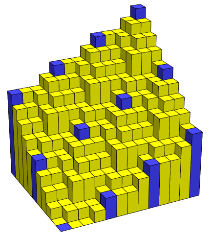
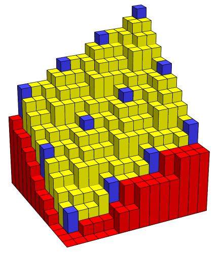
Figure 2. Left: the graph of a ZILP function $f:\mathbb{N}^{2}\to\mathbb{N}$. The height of a bar gives the value of the function, and the origin is at the front of the picture. The periodic component has periods $4$ and $5$ in the two coordinates, as indicated by the highlighted bars; the linear part has slopes $2/4$ and $4/5$ respectively. Right: A ZILEP function comprising the same “recurrent part” together with added “transient margins.”

An important preliminary step in the proofs of Theorems 1.1, 1.2 and 1.3 will be to characterize the functions that can be computed by abelian processors (as well as by the bounded and recurrent varieties). The characterizations turn out to be quite simple. A function $F:\mathbb{N}^{k}\to\mathbb{N}^{\ell}$ is computed by some finite abelian processor if and only if: (i) it maps the zero vector $\mathbf{0}\in\mathbb{N}^{k}$ to $\mathbf{0}\in\mathbb{N}^{\ell}$; (ii) it is (weakly) increasing; and (iii) it can be expressed as a linear function plus an eventually periodic function (see Definition 2.3 for precise meanings). We call a function satisfying (i)–(iii) ZILEP (zero at zero, increasing, linear plus eventually periodic). On the other hand, a function is computed by some recurrent finite abelian processor if it is ZILP: eventually periodic is replaced with periodic. Figure 2 shows examples of ZILP and ZILEP functions of two variables, illustrating some of the difficulties to be overcome in computing them by networks.

Our main theorems may be recast in terms of functions rather than processors. Table 2 summarizes our main results from this perspective. For instance, the following is a straightforward consequence of Theorem 1.3.

Corollary 1.5.

(Recurrent abelian functions) Let $\mathcal{R}$ be the smallest set of functions $F:\mathbb{N}^{k}\to\mathbb{N}$ containing the constant function $1$ and the coordinate functions $x_{1},\ldots,x_{k}$, and closed under addition and compositions of the form $F\mapsto\left\lfloor{F/\lambda}\right\rfloor$ for integer $\lambda\geq 2$. Then $\mathcal{R}$ is the set of all increasing functions $\mathbb{N}^{k}\to\mathbb{N}$ expressible as $L+P$ where $L,P:\mathbb{N}^{k}\to\mathbb{Q}$ with $L$ linear and $P$ periodic.

Components	L	+	P	Theorem(s)
(splitter and adder only)	linear	+	zero	Lemma 2.8
presink, delayer	linear	+	eventually constant	1.2, 5.3
$\lambda$-toppler	linear	+	periodic	1.3, 2.5
$\lambda$-toppler, presink, delayer	linear	+	eventually periodic	1.1, 2.4

Table 2. Four different classes of abelian network. The second column indicates the class of increasing functions $L+P:\mathbb{N}^{k}\to\mathbb{N}^{\ell}$ computable by a finite, directed acyclic abelian network whose components are splitters, adders and the gates listed in the first column. In the first two lines $L$ and $P$ take values in $\mathbb{N}^{\ell}$, while in the last two lines $L$ and $P$ take values in $\mathbb{Q}^{\ell}$.

1.4. Outline of article

Section 2 identifies the classes of functions computable by abelian processors, as described above, and formalizes the definitions and claims relating to abelian networks. Section 3 contains a few elementary reductions including the proof of Proposition 1.4. The core of the paper is Sections 4, 5 and 6, which are devoted respectively to the proofs of Theorems 1.3, 1.2 and 1.1. These proofs are by induction on the number of inputs to the processor; Theorem 1.1 is by far the hardest. A recurring theme in the proofs is meagerization, which amounts to use of the easily verified identity

$$x=\left\lfloor{\frac{x}{m}}\right\rfloor+\left\lfloor{\frac{x+1}{m}}\right\rfloor+\cdots+\left\lfloor{\frac{x+m-1}{m}}\right\rfloor$$ (2)

for positive integers $x$ and $m$. A key step in the proof of the general emulation result, Theorem 1.1, is the introduction of a ZILP function that computes the minimum of its $n$ arguments provided they are not too far apart (Proposition 6.3). That this function in turn can be emulated follows from the recurrent case, Theorem 1.3.

In Section 7 we show that no gates can be omitted from our list. We conclude by posing some open problems in Section 8.

2. Functions computed by abelian processors and networks

In preparation for the proofs of the main results about emulation, we begin by identifying the classes of functions that need to be computed.

2.1. Abelian processors

If $\mathcal{P}$ is an abelian processor with input alphabet $A$, and $w=i_{1}\cdots i_{\ell}$ is a word with letters in $A$, then we define the transition and output maps corresponding to the word:

$$t_{w}:=t_{i_{\ell}}\cdots t_{i_{1}};$$

$$o_{w}:=o_{i_{1}}+o_{i_{2}}t_{i_{1}}+o_{i_{3}}t_{i_{2}}t_{i_{1}}+\cdots+o_{i_{\ell}}t_{i_{\ell-1}}\cdots t_{i_{1}}.$$

Lemma 2.1.

For any words $w,w^{\prime}$ such that $w^{\prime}$ is a permutation of $w$, we have $t_{w}=t_{w^{\prime}}$ and $o_{w}=o_{w^{\prime}}$.

This follows from the definition of an abelian processor, by induction on the length of $w$.

The function $f=f_{\mathcal{P}}$ computed by an abelian processor $\mathcal{P}$ with initial state $q^{0}$ is given by

$$f(\mathbf{x})=o_{w(\mathbf{x})}(q^{0}),\qquad\mathbf{x}\in\mathbb{N}^{A},$$

where $w(\mathbf{x})$ is any word that contains $x_{i}$ copies of the letter $i$ for all $i\in A$. We denote vectors by boldface lower-case letters, and their coordinates by the corresponding lightface letter, subscripted.

Lemma 2.2.

Let $f=f_{\mathcal{P}}$. If $t_{\mathbf{y}}(q^{0})=t_{\mathbf{y}^{\prime}}(q^{0})$ then for any $\mathbf{x},\mathbf{y},\mathbf{y}^{\prime}\in\mathbb{N}^{k}$

$$f(\mathbf{x}+\mathbf{y})-f(\mathbf{y})=f(\mathbf{x}+\mathbf{y}^{\prime})-f(\mathbf{y}^{\prime}).$$

Let $t_{\mathbf{y}}(q^{0})=t_{\mathbf{y}^{\prime}}(q^{0})=q$; then $f(\mathbf{x}+\mathbf{y})=f(\mathbf{y})+o_{w(\mathbf{x})}(q)$ and $f(\mathbf{x}+\mathbf{y})=f(\mathbf{y}^{\prime})+o_{w(\mathbf{x})}(q)$. In other words, since $\mathbf{y}$ and $\mathbf{y}^{\prime}$ leave $\mathcal{P}$ in the same state $q$, the subsequent input of $\mathbf{x}$ has the same effect.

Definition 2.3.

A function $f:\mathbb{N}^{k}\to\mathbb{N}^{\ell}$ is (weakly) increasing if $\mathbf{x}\leq\mathbf{y}$ implies $f(\mathbf{x})\leq f(\mathbf{y})$ where $\leq$ denotes the coordinatewise partial ordering. A function $P:\mathbb{N}^{k}\to\mathbb{Q}^{\ell}$ is periodic if there is a subgroup $\Lambda\subset\mathbb{Z}^{k}$ of finite index such that $P(\mathbf{x})=P(\mathbf{y})$ whenever $\mathbf{x}-\mathbf{y}\in\Lambda$. A function $P$ is eventually periodic if there exist $\lambda_{1},\ldots,\lambda_{k}\geq 1$ and $r_{1},\ldots,r_{k}$ such that for each $i=1,\ldots,k$, if $\mathbf{x}\geq r_{i}\mathbf{e}_{i}$ then

$$P(\mathbf{x})=P(\mathbf{x}+\lambda_{i}\mathbf{e}_{i}).$$ (3)

Here $\mathbf{e}_{i}$ is the $i$th standard basis vector.

Note that given $\boldsymbol{\lambda}$ and $\mathbf{r}$, an eventually periodic function is determined by its values on the box $[0,r_{1}+\lambda_{1}]\times\cdots\times[0,r_{k}+\lambda_{k}]$. This notion of eventually periodic is intermediate in strength. A stronger requirement would be that $P$ agrees with some periodic function outside a finite set. A weaker requirement would be that (3) holds only for $\mathbf{x}\geq\mathbf{r}$.

An eventually periodic function is not generally periodic outside any finite box. The reason is that there are typically infinitely many grid points $\mathbf{x}$ (that would, e.g., be red in Figure 2) which satisfy $\mathbf{x}\geq r_{i}\mathbf{e}_{i}$ for some but not all $i$.

Theorem 2.4.

Let $k,\ell\geq 1$. A function $f:\mathbb{N}^{k}\to\mathbb{N}^{\ell}$ can be computed by a finite abelian processor if and only if $f$ satisfies all of the following.

1. $f(\mathbf{0})=0$.

2. $f$ is increasing.

3. $f=L+P$ for a linear function $L$ and an eventually periodic function $P$.

As mentioned earlier, we call a function satisfying (i)–(iii) ZILEP. Note that $L$ and $P$ need not have integer-valued coordinates, and $P$ need not be nonnegative. For example, the function $f(x)=\left\lfloor{x/2}\right\rfloor$ is ZILEP (in fact ZILP) with $L(x)=x/2$ and $P(x)=-\mathbbm{1}[x\text{ is odd}]/2$.

[Proof of Theorem 2.4] Any $f=f_{\mathcal{P}}$ trivially satisfies $f(\mathbf{0})=0$. To see that $f$ is increasing, given $\mathbf{x}\leq\mathbf{y}$ there are words $w(\mathbf{x})$ and $w(\mathbf{y})$ (where the number of occurrences of letter $i$ in $w(\mathbf{z})$ is $z_{i}$) for which $w(\mathbf{x})$ is a prefix of $w(\mathbf{y})$. Then

$$o_{w(\mathbf{x})}+o_{u}t_{w(\mathbf{x})}=o_{w(\mathbf{y})}.$$

Since the second term on the left is nonnegative, $o_{w(\mathbf{x})}(q)\leq o_{w(\mathbf{y})}(q)$.

To prove (iii), note that since $Q$ is finite, some power of $t_{i}$ is idempotent, that is

$$t_{i}^{2\lambda_{i}}=t_{i}^{\lambda_{i}}$$

for some $\lambda_{i}\geq 1$. Let $L:\mathbb{N}^{k}\to\mathbb{N}^{\ell}$ be the linear function sending

$$\lambda_{i}\mathbf{e}_{i}\mapsto f(2\lambda_{i}\mathbf{e}_{i})-f(\lambda_{i}\mathbf{e}_{i})$$

for each $i=1,\ldots,k$. Now we apply Lemma 2.2 with $\mathbf{y}=\lambda_{i}\mathbf{e}_{i}$ and $\mathbf{y}^{\prime}=2\mathbf{y}$ to get

$$f(\mathbf{z}+\lambda_{i}\mathbf{e}_{i})-f(\mathbf{z})=f(2\lambda_{i}\mathbf{e}_{i})-f(\lambda_{i}\mathbf{e}_{i})\qquad\text{for all }\mathbf{z}\geq\lambda_{i}\mathbf{e}_{i},$$ (4)

which shows that $f-L$ is eventually periodic. Thus $f$ satisfies (i)–(iii).

Conversely, given an increasing $f=L+P$, define an equivalence relation on $\mathbb{N}^{k}$ by $\mathbf{y}\equiv\mathbf{y}^{\prime}$ if $f(\mathbf{y}+\mathbf{z})-f(\mathbf{y})=f(\mathbf{y}^{\prime}+\mathbf{z})-f(\mathbf{y}^{\prime})$ for all $\mathbf{z}\in\mathbb{N}^{k}$. If $L$ is linear and $P$ is eventually periodic, then there are only finitely many equivalence classes: if $y_{i}\geq r_{i}+\lambda_{i}$ then $\mathbf{y}\equiv\mathbf{y}-\lambda_{i}\mathbf{e}_{i}$, so any $\mathbf{y}\in\mathbb{N}^{k}$ is equivalent to some element of the cuboid $[0,\lambda_{1}+r_{1}]\times\cdots\times[0,\lambda_{k}+r_{k}]$.

Now consider the abelian processor on the finite state space $\mathbb{N}^{k}/\equiv$ with $t_{i}(\mathbf{x})=\mathbf{x}+\mathbf{e}_{i}$ and $o_{i}(\mathbf{x})=f(\mathbf{x}+\mathbf{e}_{i})-f(\mathbf{x})$. Note that $t_{i}$ and $o_{i}$ are well-defined. With initial state $\mathbf{0}$, this processor computes $f$.

2.2. Recurrent abelian processors

Recall that an abelian processor is called recurrent if for any states $q,q^{\prime}\in Q$ there exists $\mathbf{x}\in\mathbb{N}^{k}$ such that $q^{\prime}=t_{\mathbf{x}}(q)$. Since we assume that every state is accessible from the initial state $q^{0}$, this is equivalent to the assertion that for every $q\in Q$ and $\mathbf{y}\in\mathbb{N}^{k}$ there exists $\mathbf{z}\in\mathbb{N}^{k}$ such that $q=t_{\mathbf{y}+\mathbf{z}}(q)$. Our next result differs from Theorem 2.4 in only two words: recurrent has been added and eventually has been removed! As mentioned earlier, we call a function satisfying (i)–(iii) below ZILP.

Theorem 2.5.

Let $k,\ell\geq 1$. A function $f:\mathbb{N}^{k}\to\mathbb{N}^{\ell}$ can be computed by a recurrent finite abelian processor if and only if $f$ satisfies all of the following.

1. $f(\mathbf{0})=0$.

2. $f$ is increasing.

3. $f=L+P$ for a linear function $L$ and a periodic function $P$.

By Theorem 2.4, $f$ satisfies (i) and (ii) and $f=L+P$ with $L$ linear and $P$ eventually periodic. To prove (iii) we must show that equation (4) holds for all $\mathbf{z}\in\mathbb{N}^{k}$. By recurrence, for any $\mathbf{y}\in\mathbb{N}^{k}$ and any $i\in A$ there exists $\mathbf{y}^{\prime}\geq\lambda_{i}\mathbf{e}_{i}$ such that $t_{\mathbf{y}^{\prime}}(q)=t_{\mathbf{y}}(q)$. Now taking $\mathbf{x}=\lambda_{i}\mathbf{e}_{i}$ in Lemma 2.2, the linear terms cancel, leaving

$$P(\mathbf{y}+\lambda_{i}\mathbf{e}_{i})-P(\mathbf{y})=P(\mathbf{y}^{\prime}+\lambda_{i}\mathbf{e}_{i})-P(\mathbf{y}^{\prime}).$$

The right side vanishes since $P$ is eventually periodic. Since $\mathbf{y}\in\mathbb{N}^{k}$ was arbitrary, $P$ is in fact periodic.

Conversely, given an increasing $f=L+P$, we define an abelian processor $\mathcal{P}$ on state space $\mathbb{N}^{k}/\equiv$ as in the proof of Theorem 2.4. If $L$ is linear and $P$ is periodic, then for each $i=1,\ldots,k$ we have $\mathbf{y}\equiv\mathbf{y}-\lambda_{i}\mathbf{e}_{i}$ whenever $y_{i}\geq\lambda_{i}$. Now given any $\mathbf{x},\mathbf{y}\in\mathbb{N}^{k}$ we find $\mathbf{x}^{\prime}\equiv\mathbf{x}$ with $\mathbf{x}^{\prime}\geq\mathbf{y}$, so $\mathcal{P}$ is recurrent.

2.3. Abelian networks

An abelian network ${\mathcal{N}}$ is a directed multigraph $G=(V,E)$ along with specified pairwise disjoint sets $I,O,T\subset E$ of input, output and trash edges respectively. These edges are dangling: the input edges have no tail, while the output and trash edges have no head. The trash edges are for discarding unwanted letters. Each node $v\in V$ is labeled with an abelian processor $\mathcal{P}_{v}$ whose input alphabet equals the set of incoming edges to $v$ and whose output alphabet is the set of outgoing edges from $v$. In this paper, all abelian networks are assumed finite: $G$ is a finite graph and each $\mathcal{P}_{v}$ is a finite processor.

An abelian network operates as follows. Its total state is given by the internal states $(q_{v})_{v\in V}$ of all its processors $\mathcal{P}_{v}$, together with a vector $\mathbf{x}=(x_{e})_{e\in E}\in\mathbb{N}^{E}$ that indicates the number of letters sitting on each edge, waiting to be processed. Initially, $\mathbf{x}$ is supported on the set of input edges $I$. At each step, any non-output non-trash edge $e$ with $x_{e}>0$ is chosen, and a letter is fed into the processor at its endnode $v$. Thus, $x_{e}$ is decreased by $1$, the state of $\mathcal{P}_{v}$ is updated from $q_{v}$ to $t_{e}(q_{v})$, and $\mathbf{x}$ is increased by $o_{e}(q_{v})$ (interpreted as a vector in $\mathbb{N}^{E}$ supported on the outgoing edges from $v$). Here $t$ and $o$ are the maps associated to $\mathcal{P}_{v}$. The sequence of choices of the edges $e$ at successive steps is called a legal execution. The execution is said to halt if, after some finite number of steps, $\mathbf{x}$ is supported on the set of output and trash edges (so that there are no letters left to process).

The following facts are proved in [BL16a, Theorem 4.7]. Fixing the initial internal states $\mathbf{q}^{0}=(q_{v}^{0})_{v\in V}$ and an input vector $\mathbf{x}\in\mathbb{N}^{I}$, if some execution halts then all legal executions halt. In the latter case, the final states of the processors and the final output vector do not depend on the choice of legal execution.

Suppose for a given $\mathbf{q}^{0}$ that the network halts on all input vectors. Then, since the final output vector depends only on the input vector, the abelian network computes a function $\mathbb{N}^{I}\to\mathbb{N}^{O}$. If a network ${\mathcal{N}}$ and a processor $\mathcal{P}$ compute the same function, then we say that ${\mathcal{N}}$ emulates $\mathcal{P}$.

Proposition 2.6.

If a finite abelian network halts on all inputs, then it emulates some finite abelian processor.

We can regard the entire network as a processor, with its state given by the vector of internal states $\mathbf{q}=(q_{v})_{v\in V}$. Its transition and output maps are determined by feeding in a single input letter, performing any legal execution until it halts, and observing the resulting state and output letters. Feeding in two input letters and using (a special case of) the insensitivity to execution order stated above, we see that the relations (1) hold, so the processor is abelian.

The abelian networks that halt on all inputs are characterized in [BL16b, Theorem 5.6]: they are those for which a certain matrix called the production matrix has Perron-Frobenius eigenvalue strictly less than $1$. An abelian network is called directed acyclic if its graph $G$ has no directed cycles; such a network trivially halts on all inputs. This paper is mostly concerned with directed acyclic networks, together with some networks with certain limited types of feedback; all of them halt on all inputs.

2.4. Recurrent abelian networks

The next lemma follows from [BL16c, Theorem 3.9], but we include a proof for the sake of completeness. A processor is called immutable if it has just one state, and mutable otherwise. Among the abelian logic gates in Table 1, splitters and adders are immutable; topplers, delayers and presinks are mutable.

Recall (from Proposition 1.4 or Figure 3) that if feedback is permitted, then the transient ${\tt delayer}$ gate can be emulated by a network of recurrent gates, namely a $2$-${\tt toppler}$ and a ${\tt splitter}$. The next result shows that without feedback, no transient processor can be emulated by a network of recurrent processors.

Proposition 2.7.

A directed acyclic network ${\mathcal{N}}$ of recurrent processors emulates a recurrent processor.

We proceed by induction on the number $m$ of mutable processors in ${\mathcal{N}}$. In the case $m=0$, the network ${\mathcal{N}}$ has only one state, so it is trivially recurrent.

For the inductive step, suppose $m\geq 1$. Since ${\mathcal{N}}$ is directed acyclic, it has a mutable processor $\mathcal{P}$ such that no other mutable processor feeds into anything upstream of $\mathcal{P}$. If ${\mathcal{N}}$ has $k$ inputs, we can regard the remainder ${\mathcal{N}}-\mathcal{P}$ as a network with $m{-}1$ mutable processors and $k{+}k^{\prime}$ inputs, where $k^{\prime}$ is the number of edges from $\mathcal{P}$ to ${\mathcal{N}}-\mathcal{P}$. For each state $q$ of ${\mathcal{N}}$, the function $f=f_{{\mathcal{N}},q}$ has the form

$$f(\mathbf{x})=g(\mathbf{x},h(\mathbf{x}))+j(\mathbf{x})$$

where $g:\mathbb{N}^{k+k^{\prime}}\to\mathbb{N}^{\ell}$ is the function computed by ${\mathcal{N}}-\mathcal{P}$ in initial state $q$; and $h:\mathbb{N}^{k}\to\mathbb{N}^{k^{\prime}}$ and $j:\mathbb{N}^{k}\to\mathbb{N}^{\ell}$ are the functions sent by $\mathcal{P}$ in initial state $q$ to ${\mathcal{N}}-\mathcal{P}$ and the output of ${\mathcal{N}}$, respectively.

By Theorem 2.5 and the inductive hypothesis, each of $g,h,j$ is the sum of a periodic and a linear function. Writing $g(\mathbf{y})=P(\mathbf{y})+\mathbf{b}\cdot\mathbf{y}$ and $h(\mathbf{x})=Q(\mathbf{x})+\mathbf{c}\cdot\mathbf{x}$ we have

$$f(\mathbf{x})=P(\mathbf{x},Q(\mathbf{x})+\mathbf{c}\cdot\mathbf{x})+\mathbf{b}\cdot(\mathbf{x},Q(\mathbf{x})+\mathbf{c}\cdot\mathbf{x})+j(\mathbf{x}).$$

The first term is periodic and the second is a linear function plus a periodic function. Since $q$ is arbitrary the proof is complete by Theorem 2.5.

2.5. Varying the initial state

We remark that the emulation claims of our main theorems can be strengthened slightly, in the following sense. Our definition of a processor $\mathcal{P}$ included a designated initial state $q^{0}$, but one may instead consider starting $\mathcal{P}$ from any state $q\in Q$, and it may compute a different function from each $q$. All of these functions can be computed by the same network ${\mathcal{N}}$, by varying the internal states of the gates in ${\mathcal{N}}$. To set up the network ${\mathcal{N}}$ to compute the function $f_{\mathcal{P},q}$, we simply choose an input vector $\mathbf{x}$ that causes $\mathcal{P}$ to transition from $q^{0}$ to $q$, then feed $\mathbf{x}$ to ${\mathcal{N}}$ and observe the resulting gate states. In the recurrent case, this amounts to adjusting the priming of topplers. In the transient case, a “used” delayer can be replaced with a wire, while a used presink becomes a trash edge.

2.6. Splitter-adder networks

In this section we show that splitter-adder networks compute precisely the increasing linear functions. Using this, we will see how Theorem 1.3 implies Corollary 1.5.

Lemma 2.8.

Let $k,\ell\geq 1$. The function $f:\mathbb{N}^{k}\to\mathbb{N}^{\ell}$ can be computed by a network of splitters and adders if and only if $f(\mathbf{x})=L\mathbf{x}$ for some nonnegative integer $\ell\times k$ matrix $L$.

If a network of splitters and adders has a directed cycle, then it does not halt on all inputs, and so does not “compute a function” according to our definition. If the network is directed acyclic then by Propositions 2.7 and 2.5 it computes a ZILP function. Since the network is immutable, the periodic part of any linear + periodic decomposition must be zero. Conversely, consider a network of $k$ splitters $\mathcal{S}_{i}$ and $\ell$ adders $\mathcal{A}_{j}$, with $L_{ji}$ edges from $\mathcal{S}_{i}$ to $\mathcal{A}_{j}$. Feed each input $i$ into $\mathcal{S}_{i}$, and feed each $\mathcal{A}_{j}$ into output $j$.

[Proof of Corollary 1.5] Given a function $F\in\mathcal{R}$, the function $\mathbf{x}\mapsto F(\mathbf{x})-F(\mathbf{0})$ can be computed by a finite, directed acyclic network of splitters, adders and (possibly primed) topplers. By Proposition 2.7 any such network emulates a recurrent finite abelian processor, so $F$ has the desired form by Theorem 2.5.

Conversely if $F=L+P$ with $L$ linear and $P$ periodic, then $F(\mathbf{x})-F(\mathbf{0})$ is computable by a finite directed acyclic network of splitters, adders and topplers by Theorem 1.3. We induct on the number of topplers to show that $F\in\mathcal{R}$. In the base case there are no topplers, ${\mathcal{N}}$ is a splitter-adder network, so by Lemma 2.8, $F$ is an increasing linear function of its inputs $x_{1},\ldots,x_{k}$.

Assume now that at least one component of ${\mathcal{N}}$ is a toppler. Since ${\mathcal{N}}$ is directed acyclic, there is a toppler $\mathcal{T}$ such that no other toppler is downstream of $\mathcal{T}$. Write $\mathcal{D}$ for the portion of ${\mathcal{N}}$ downstream of $\mathcal{T}$, and $\mathcal{U}={\mathcal{N}}-\mathcal{T}-\mathcal{D}$ for the remainder of the network. Suppose $\mathcal{U}$ sends outputs $r,s,\mathbf{u}$ respectively to the output of ${\mathcal{N}}$, to $\mathcal{T}$, and to $\mathcal{D}$; and that the toppler $\mathcal{T}$ sends output $t$ to $\mathcal{D}$.

The downstream part $\mathcal{D}$ consists of only splitters and adders, so it computes a linear function

$$L(t,\mathbf{u})=at+\mathbf{b}\cdot\mathbf{u}$$

for some $a\in\mathbb{N}$ and $\mathbf{b}\in\mathbb{N}^{j}$, where $j$ is the number of edges from $\mathcal{U}$ to $\mathcal{D}$. The total output of ${\mathcal{N}}$ is

$$F(\mathbf{x})-F(\mathbf{0})=r+L(t,\mathbf{u})=r+a\left\lfloor{\frac{s}{\lambda}}\right\rfloor+\mathbf{b}\cdot\mathbf{u}.$$

Each of $r,s,\mathbf{u}$ is a function of the input $\mathbf{x}=(x_{1},\ldots,x_{k})$. By induction, $r$ and $s$ and each $u_{i}$ belongs to the class $\mathcal{R}$, so $F$ does as well.

3. Basic reductions

In this section we describe some elementary network reductions.

3.1. Multi-way splitters and adders

An $n$-splitter computes the function $\mathbb{N}\to\mathbb{N}^{n}$ sending $x\mapsto(x,\ldots,x)$. It is emulated by a directed binary tree of $n-1$ splitters with the input node at the root and the $n$ output nodes at the leaves. Similarly, an $n$-adder computes the function $\mathbb{N}^{n}\to\mathbb{N}$ given by $(x_{1},\ldots,x_{n})\mapsto x_{1}+\cdots+x_{n}$. It is emulated by a tree of $n-1$ adders.

3.2. The power of feedback

[Proof of Proposition 1.4] To emulate an unprimed $\lambda$-toppler, let $r=\left\lceil{\log_{2}\lambda}\right\rceil$ and let

$$2^{r}-\lambda=\sum_{i=0}^{r-2}b_{i}2^{i},\qquad b_{i}\in\{0,1\}$$

be the binary representation of $2^{r}-\lambda$. Consider $r$ $2$-topplers $H_{0},H_{1},\ldots,H_{r-1}$ in series: the input node is $H_{0}$, and each $H_{i}$ feeds into $H_{i+1}$ for $0\leq i<r{-}1$. For $i<r-1$ the $2$-toppler $H_{i}$ is primed with $b_{i}$. The last $2$-toppler $H_{r-1}$ is unprimed, and feeds into an $s$-splitter ($s=1+\sum_{i=0}^{r-1}b_{i}$) which feeds one letter each into the output node $o$ and the nodes $H_{i}$ such that $b_{i}=1$. This network repeatedly counts in binary from $2^{r}-\lambda$ to $2^{r}-1$, and it sends output precisely when it transitions from $2^{r}-1$ back to $2^{r}-\lambda$. Hence, it emulates a $\lambda$-toppler. See Figure 3 for examples.

We can emulate a $q$-primed $\lambda$-toppler using the same network, but with different initial states for its $2$-topplers. The required states are simply those that result from feeding $q$ input letters into the network described above.

A delayer is constructed by splitting the output of a $2$-toppler and adding one branch back in as input to the $2$-toppler (Figure 3).

3.3. Primed topplers

The following shows that we can also do without primed topplers (at the expense of using a transient gate: the presink).

Lemma 3.1.

A primed $\lambda$-toppler can be emulated by a directed acyclic network comprising an unprimed $\lambda$-toppler, adders, splitters, and a presink.

See Figure 4. For $0\leq q<\lambda$ we have $\lfloor(x+q)/\lambda\rfloor=\lfloor(x+q(x-1)^{+})/\lambda\rfloor$, so we can emulate a $q$-primed $\lambda$-toppler by splitting the input, feeding it into a presink, and adding $q$ copies of the result into the original input before sending it to an unprimed $\lambda$-toppler.

	$\Longleftrightarrow$
	$\Longleftrightarrow$
	$\Longleftrightarrow$
	$\Longleftrightarrow$

Figure 3. Emulating a $3$-toppler, $4$-toppler, $5$-toppler and delayer by networks of $2$-topplers.

$\Longleftrightarrow$

Figure 4. Emulating a primed toppler with an unprimed toppler.

3.4. Reduction to unary output

Let $\mathcal{P}$ be an abelian processor that computes $f:\mathbb{N}^{k}\to\mathbb{N}^{\ell}$. If $\ell=1$ then we say that $\mathcal{P}$ has unary output. All of the logic gates in Table 1 have unary output with the exception of the splitter. The next lemma shows that, for rather trivial reasons, it is enough to emulate processors with unary output.

Lemma 3.2.

Any abelian processor can be emulated by a directed acyclic network of splitters and processors with unary output.

Let $\mathcal{P}$ compute $f=(f_{1},\ldots,f_{\ell}):\mathbb{N}^{k}\to\mathbb{N}^{\ell}$. By ignoring all outputs of $\mathcal{P}$ except the $j$th, we obtain an abelian processor $\mathcal{P}_{j}$ that computes $f_{j}$. Each $\mathcal{P}_{j}$ has unary output, and $\mathcal{P}$ is emulated by a network that sends each input into an $\ell$-splitter that feeds into $\mathcal{P}_{1},\ldots,\mathcal{P}_{\ell}$ (Figure 5).

Figure 5. Emulating a $2$-output abelian processor with two unary-output processors.

In the subsequent proofs we can thus assume that the processors to be emulated have unary output. By a $k$-ary processor we mean one with $k$ inputs. A $1$-ary processor is sometimes called unary.

4. The recurrent case

In this section we prove Theorem 1.3. By Lemma 3.2 we may assume that the recurrent processor to be emulated has unary output. We will proceed by induction on the number of inputs.

4.1. Unary case

We start with the unary case (i.e. one input), which will form the base of our induction. An alternative would be to start the induction with the trivial case of zero inputs, but the simplicity of the unary case is illustrative.

By Theorem 2.5, a recurrent unary processor computes an increasing function $f:\mathbb{N}\to\mathbb{N}$ of the form $f(x)=cx+P(x)$, where $c\in\mathbb{Q}_{\geq 0}$ and $P:\mathbb{N}\to\mathbb{Q}$ is periodic.

Lemma 4.1.

Let $\mathcal{P}$ be a recurrent unary processor that computes $f(x)=cx+P(x)$, where $P$ is periodic of period $\lambda$. Then $\mathcal{P}$ can be emulated by a network of adders, splitters and (suitably primed) $\lambda$-topplers.

Observe first that $c\lambda$ is an integer: since $f(0)=0$, we have $P(\lambda)=P(0)=0$ thus $f(\lambda)=c\lambda\in\mathbb{N}$. We construct a network of $c\lambda$ parallel $\lambda$-topplers as follows: the (unary) input is split (by a $c\lambda$-splitter) into $c\lambda$ streams, each of which feeds into a separate $\lambda$-toppler. The outputs of the topplers are then combined (by a $c\lambda$-adder) to a single output (Figure 6).

After $m\lambda$ letters are input to this network, $m\in\mathbb{N}$, each toppler will return to its original state having output $m$ letters, for a total output of $m\times c\lambda=c(m\lambda)$; thus the network does compute $cx+Q(x)$ where $Q$ has period $\lambda$ or some divisor of $\lambda$. To force $Q=P$ it suffices to choose the initial state $q$ in such a way that the network’s output for $x=1,2,\dots,\lambda$ matches $f(1),\dots,f(\lambda)$. This is easily done by setting $d_{i}=f(x)-f(x{-}1)$, and for each $i$ with $1\leq i\leq\lambda$, starting $d_{i}$ topplers in state $\lambda{-}i$.

Figure 6 illustrates the network constructed to compute the function $f=\frac{3}{4}x+P(x)$ where $P$ has period 4 with $P(0)=0$, $P(1)=\frac{1}{4}$, $P(2)=\frac{6}{4}$ and $P(3)=\frac{3}{4}$. The values of $f$ begin $0,1,3,3,3,4,6,6,6,7,9,9,9,\dots$. The “I/O diagram” of $f$ is shown at the top of the figure; dots represent input letters and bars are output letters; the unfilled circle represents the initial state.

Figure 6. Emulating a unary processor with a network of primed topplers.

4.2. Reduction to the meager case

A recurrent $k$-ary processor computes a function $f:\mathbb{N}^{k}\to\mathbb{N}$ of the form $f(\mathbf{x})=\mathbf{b}\cdot\mathbf{x}+P(\mathbf{x})$ where $P$ is periodic.

Definition 4.2.

A recurrent processor is nondegenerate if $b_{i}\neq 0$ for all $i$.

Note that if $b_{i}=0$ then $f(\mathbf{x})$ does not depend on the coordinate $x_{i}$. In this case, by Theorem 2.5 there is a finite $(k{-}1)$-ary recurrent processor that computes $f$.

Denote the lattice of periodicity of $P$ by $\Lambda\subset\mathbb{Z}^{k}$. Let $\lambda_{i}$ be the smallest positive integer such that $\lambda_{i}\mathbf{e}_{i}\in\Lambda$. For the purposes of the forthcoming induction, we focus on the last coordinate.

Definition 4.3.

We say that a $k$-ary processor $\mathcal{P}$ is meager if $f_{\mathcal{P}}(\lambda_{k}\mathbf{e}_{k})=1$.

Note that if $\mathcal{P}$ is meager then for all $\mathbf{x}\in\mathbb{N}^{k}$ we have

$$f_{\mathcal{P}}(\mathbf{x}+\lambda_{k}\mathbf{e}_{k})=f_{\mathcal{P}}(\mathbf{x})+1.$$

Next we emulate a nondegenerate recurrent processor by a network of meager processors.

Lemma 4.4.

Let $\mathcal{P}$ be a nondegenerate recurrent $k$-ary processor and let $m=f_{\mathcal{P}}(\lambda_{k}\mathbf{e}_{k})=\lambda_{k}b_{k}$. Then $\mathcal{P}$ can be emulated by a network of $m-1$ splitters, $m-1$ adders, and $m$ meager recurrent $k$-ary processors.

For each $j=0,\ldots,m-1$ consider the function

$$f_{j}(\mathbf{x})=\left\lfloor{\frac{f(\mathbf{x})+j}{m}}\right\rfloor.$$

We claim that $f_{j}=f_{\mathcal{P}_{j}}$ for some recurrent processor $\mathcal{P}_{j}$. One way to prove this is to use Theorem 2.5, checking from the above formula that since $f$ is ZILP, $f_{j}$ is also ZILP. Another route is to note that $f_{j}$ is computed by a network in which the output of $\mathcal{P}$ is fed into a $j$-primed $m$-toppler. By Proposition 2.7, $f_{j}$ is therefore computed by some recurrent processor. (Note however that this network itself will not help us to emulate $\mathcal{P}$ using gates, since it contains $\mathcal{P}$!) Figure 7 illustrates an example of the reduction.

Now we use the meagerization identity (2):

$$f=\left\lfloor{\frac{f}{m}}\right\rfloor+\left\lfloor{\frac{f+1}{m}}\right\rfloor+\cdots+\left\lfloor{\frac{f+m-1}{m}}\right\rfloor$$

Thus, $\mathcal{P}$ is emulated by an $m$-splitter that feeds into $\mathcal{P}_{0},\ldots,\mathcal{P}_{m-1}$, with the results fed into an $m$-adder. It remains to check that each $\mathcal{P}_{j}$ is meager. We have

$$f_{j}(\mathbf{x}+\lambda_{k}\mathbf{e}_{k})=\left\lfloor{\frac{f(\mathbf{x}+\lambda_{k}\mathbf{e}_{k})+j}{m}}\right\rfloor=\left\lfloor{\frac{f(\mathbf{x})+\lambda_{k}b_{k}+j}{m}}\right\rfloor=f_{j}(\mathbf{x})+1.$$

Figure 7. Left: Example state diagram of a recurrent binary processor $\mathcal{P}$ with $\lambda=(4,5)$ and $b=(\frac{1}{2},\frac{4}{5})$. (The function is the same as the one in Figure 2 (left)). A dot with coordinates $\mathbf{x}=(x_{1},x_{2})$ represents the state of the processor after it has received input $\mathbf{x}$. (The initial state $(0,0)$ is an unfilled circle.) Each solid contour line between two adjacent dots indicates that a letter is emitted when making that transition. Right: The highlighted contours form the state diagram of the corresponding meager processor $\mathcal{P}_{3}$, obtained by keeping every fourth contour (starting from the first) of the left picture. The vertical period is still $5$, although the horizontal period has increased.

4.3. Reducing the alphabet size

Now we come to the main reduction.

Lemma 4.5.

Let $\mathcal{P}$ be a meager recurrent $k$-ary processor satisfying $f_{\mathcal{P}}(\mathbf{x}+\lambda_{k}\mathbf{e}_{k})=f_{\mathcal{P}}(\mathbf{x})+1$. Then $\mathcal{P}$ can be emulated by a network of a recurrent $(k{-}1)$-ary processor, a $\lambda_{k}$-toppler, and an adder.

Let $\mathcal{P}$ compute $f$. By Theorem 2.5, $f$ is ZILP. Its representation as a linear plus a periodic function makes sense as a function on all of $\mathbb{Z}^{k}$. Now consider the increasing function

$$g(x_{1},\ldots,x_{k-1})=-c-\min\{x_{k}\in\mathbb{Z}\,:\,f(x_{1},\ldots,x_{k})\geq 0\}.$$

where $c=-\min\{x_{k}\in\mathbb{Z}\,:\,f(0,\ldots,0,x_{k})\geq 0\}$. Note that $g$ is an increasing function of $(x_{1},\ldots,x_{k-1})\in\mathbb{N}^{k-1}$, and $g(\mathbf{0})=0$.

If $\boldsymbol{\lambda}\in\lambda_{1}\mathbb{Z}\times\cdots\times\lambda_{k-1}\mathbb{Z}\times\{0\}$, then

$$g(\mathbf{x}+\boldsymbol{\lambda}) =-c-\min\{x_{k}\in\mathbb{Z}\,:\,f(x_{1},\ldots,x_{k})+\mathbf{b}\cdot\boldsymbol{\lambda}\geq 0\}$$

$$=-c-\min\{x_{k}\in\mathbb{Z}\,:\,f(x_{1},\ldots,x_{k-1},x_{k}+\lambda_{k}(\mathbf{b}\cdot\boldsymbol{\lambda}))\geq 0\}$$

$$=g(\mathbf{x})+\lambda_{k}(\mathbf{b}\cdot\boldsymbol{\lambda})$$

where the second equality holds because $\mathcal{P}$ is meager. Hence $g$ is ZILP. Let $\mathcal{Q}$ be the $(k-1)$-ary processor that computes $g$ (which exists by Theorem 2.5).

Note that for any integer $j$ we have that $f(x_{1},\ldots,x_{k})\geq j$ if and only if $f(\mathbf{x}-j\lambda_{k}\mathbf{e}_{k})\geq 0$, which in turn happens if and only if $g(x_{1},\ldots,x_{k-1})+x_{k}+c\geq j\lambda_{k}$. Hence

$$f(x_{1},\ldots,x_{k})=\left\lfloor{\frac{g(x_{1},\ldots,x_{k-1})+x_{k}+c}{\lambda_{k}}}\right\rfloor.$$

The definition of $c$ gives that $0\leq c<\lambda_{k}$, since $f(\mathbf{0})=0$ and $f(-\lambda_{k}\mathbf{e}_{k})=-1$. So $\mathcal{P}$ is emulated by the network that feeds the last input letter $a_{k}$ into a $\lambda_{k}$-toppler $\mathcal{T}$ primed with $c$, and $a_{1},\ldots,a_{k-1}$ into $\mathcal{Q}$ which feeds into $\mathcal{T}$.

Figure 8. Emulating a meager recurrent $k$-ary processor via a recurrent $(k{-}1)$-ary processor.

Now we can prove the main result in the recurrent case. [Proof of Theorem 1.3] Let $\mathcal{P}$ be a recurrent abelian processor to be emulated. By Lemma 3.2 we can assume that it has unary output. We proceed by induction on the number of inputs $k$. The base case $k=1$ is Lemma 3.2. For $k>1$, we first use Lemma 4.4 to emulate the processor by a network of meager $k$-ary processors. Then we replace each of these with a network of $(k-1)$-ary processors, by Lemma 4.5, and then apply the inductive hypothesis to each of these.

4.4. The number of gates

How many gates do our networks use? For simplicity, consider the case of a recurrent $k$-ary abelian processor with $\lambda_{i}=2$ and $b_{i}=1/2$ for all $i$. It is not difficult to check that our construction uses $O(c^{k})$ gates as $k\to\infty$ for some $c$. In fact, a counting argument shows that exponential growth with $k$ is unavoidable, as follows. Consider networks of only adders, splitters, and $2$-topplers, but suppose that we allow feedback (so that a $\lambda$-toppler can be replaced with $O(\log\lambda)$ gates, by Proposition 1.4). The number of networks with at most $n$ gates is at most $n^{c^{\prime}n}$ for some $c^{\prime}$ (we choose the type of each gate, together with the matching of inputs to outputs). On the other hand, the number of different ZILP functions $f$ that can be computed by a processor of the above-mentioned form is at least $2^{\binom{k}{\lfloor k/2\rfloor}}$, since we may choose an arbitrary value $f(\mathbf{x})\in\{0,1\}$ for each of the $\binom{k}{\lfloor k/2\rfloor}$ elements $\mathbf{x}$ of the middle layer $\{\mathbf{x}\in\{0,1\}^{k}:\sum_{i}x_{i}=\lfloor k/2\rfloor\}$ of the hypercube. If all $k$-ary processors can be emulated with at most $n$ gates then $n^{c^{\prime}n}>2^{\binom{k}{\lfloor k/2\rfloor}}$. It follows easily that some such processor requires at least $C^{k}$ gates, for some fixed $C>1$.

If we consider the dependence on the quantities $\lambda_{i}$ and $b_{i}$ as well as $k$, our construction apparently leaves more room for improvement in terms of the number of gates, since repeated meagerization tends to increase the periods $\lambda_{i}$. One might also investigate whether there is an interesting theory of $k$-ary functions that can be computed with only polynomially many gates as a function of $k$.

Our construction of networks emulating transient processors (Section 6) will be much less efficient than the recurrent case, since the induction will rely on a ZILP function of a potentially large number of arguments (Proposition 6.3) that is emulated by appeal to Theorem 1.3. It would be of interest to reduce the number of gates here.

5. The bounded case

In this section we prove Theorem 1.2. Moreover, we identify the class of functions computable without topplers.

Lemma 5.1.

Let $f:\mathbb{N}^{k}\to\{0,1\}$ be increasing with $f(\mathbf{0})=0$. There is a directed acyclic network of adders, splitters, presinks and delayers that computes $f$.

Let $M$ be the set of $\mathbf{m}\in\mathbb{N}^{k}$ that are minimal (in the coordinate partial order) in $f^{-1}(1)$. By Dickson’s Lemma [D13], $M$ is finite; and $f(\mathbf{x})=1$ if and only if $\mathbf{x}\geq\mathbf{m}$ for some $\mathbf{m}\in M$. Thus

$$f(\mathbf{x})=\bigvee_{\mathbf{m}\in M}\bigwedge_{i\in A}\mathbbm{1}[x_{i}\geq m_{i}].$$

The function $\mathbbm{1}[x_{i}\geq m_{i}]$ is computed by $m_{i}-1$ delayers in series followed by a presink. The minimum ($\wedge$) or maximum ($\vee$) of a pair of boolean ($\{0,1\}$-valued) inputs is computed by adding the inputs and feeding the result into a delayer or a presink respectively. The minimum or maximum of any finite set of boolean inputs is computed by repeated pairwise operations. See Figure 9. The lemma follows.

Figure 9. Networks computing $\mathbbm{1}[x\geq 4]$, and $\min(b_{1},b_{2},b_{3})$ and $\max(b_{1},b_{2},b_{3})$ for boolean inputs $b_{i}\in\{0,1\}$.

Lemma 5.2.

Suppose $f:\mathbb{N}^{k}\to\mathbb{N}$ is increasing and bounded with $f(\mathbf{0})=0$. Then there is a directed acyclic network of adders, splitters, presinks and delayers that computes $f$.

By Lemma 5.1, for each $j\in\mathbb{N}$ there is a network of the desired type that computes $\mathbf{x}\mapsto\mathbbm{1}[f(\mathbf{x})>j]$. If $f$ is bounded by $J$, then $f(\mathbf{x})=\sum_{j=0}^{J-1}\mathbbm{1}[f(\mathbf{x})>j]$, so we add the outputs of these $J$ networks.

[Proof of Theorem 1.2] Let $\mathcal{P}$ be a bounded abelian processor. By Lemma 3.2 we can assume that it has unary output. The function that it computes is increasing and bounded, and maps $\mathbf{0}$ to $0$. Therefore, apply Lemma 5.2.

What is the class of all functions computable by a network of adders, splitters presinks and delayers? Let us call a function $P:\mathbb{N}^{k}\to\mathbb{N}^{\ell}$ eventually constant if it is eventually periodic with all periods $1$; that is, there exist $r_{1},\ldots,r_{k}\in\mathbb{N}$ such that $P(\mathbf{x})=P(\mathbf{x}+\mathbf{e}_{i})$ whenever $\mathbf{x}_{i}\geq r_{i}$. (Note the relatively weak meaning of this term: Such a function may admit multiple limits as some arguments tend to infinity while the others are held constant, as in our remark following the definition of eventually periodic.)

Theorem 5.3.

Let $k\geq 1$. A function $f:\mathbb{N}^{k}\to\mathbb{N}$ can be computed by a finite, directed acyclic network of adders, splitters, presinks and delayers if and only if it satisfies all of the following.

1. $f(\mathbf{0})=0$.

2. $f$ is increasing.

3. $f=L+P$ for a linear function $L$ and an eventually constant function $P$.

Let ${\mathcal{N}}$ be such a network, and let it compute $f$. Since adders and splitters are immutable, and presinks and delayers become immutable after receiving one input, the internal state of ${\mathcal{N}}$ can change only a bounded number of times. In fact, for each $i=1,\ldots,k$ we have $t_{i}^{r}=t_{i}^{r+1}$ where $r$ is the total number of presinks and delayers in ${\mathcal{N}}$. Letting $b_{i}:=f((r+1)\mathbf{e}_{i})-f(r\mathbf{e}_{i})$, it follows from Lemma 2.2 that

$$f(\mathbf{x}+\mathbf{e}_{i})-f(\mathbf{x})=b_{i}$$ (5)

whenever $x_{i}\geq r$. Note that $b_{i}\in\mathbb{N}$. Letting $P(\mathbf{x}):=f(\mathbf{x})-\mathbf{b}\cdot\mathbf{x}$, we find that $P(\mathbf{x}+\mathbf{e}_{i})=P(\mathbf{x})$ whenever $x_{i}\geq r$, so $P$ is eventually constant.

Conversely, suppose that $f$ satisfies (i)-(iii). Write $f=L+P$ for a linear function $L(\mathbf{x})=\mathbf{b}\cdot\mathbf{x}$ with $\mathbf{b}\in\mathbb{N}^{k}$, and an eventually constant function $P$. Then there exist $r_{1},\ldots,r_{k}$ such that (5) holds for all $i=1,\ldots,k$ and all $\mathbf{x}\in\mathbb{N}^{k}$ such that $x_{i}\geq r_{i}$. In particular, the function

$$g(\mathbf{x}):=f(\mathbf{x})-\sum_{i=1}^{k}b_{i}(x_{i}-r_{i})^{+}$$

is ZILP and bounded. By Theorem 1.2 there is a network ${\mathcal{N}}$ of adders, splitters, presinks and delayers that computes $g$. To compute $f$, feed each input $x_{i}$ into a splitter which feeds into ${\mathcal{N}}$ and into an $r_{i}$-delayer followed by a $b_{i}$-splitter.

6. The general case

In this section we prove Theorem 1.1. As in the recurrent case, the proof will be by induction on the number of inputs, $k$, of the abelian processor. We identify $\mathbb{N}^{k}$ with $\mathbb{N}^{k-1}\times\mathbb{N}$, and write $(\mathbf{y},z)=\mathbf{y}+z\mathbf{e}_{k}$. Meagerization will again play a crucial role. A major new ingredient is “interleaving of layers”.

6.1. The unary case

As before, we first prove the case of unary input, although an alternative would be to start the induction with the trivial zero-input processor.

Lemma 6.1.

Any abelian processor with unary input and output can be emulated by a directed acyclic network of adders, splitters, topplers, presinks and delayers.

Let the processor $\mathcal{P}$ compute $F:\mathbb{N}\to\mathbb{N}$. Since $F$ is ZILEP, it is linear plus periodic when the argument is sufficiently large; thus, there exists $R\in\mathbb{N}$ such that the function $G$ given by

$$G(x):=F(x+R)-F(R),\qquad x\in\mathbb{N}$$

is ZILP. We have

$$F(x)=G\bigl{(}(x-R)^{+}\bigr{)}+\sum_{i=0}^{R-1}\bigl{[}F(i+1)-F(i)\bigr{]}\,\mathbbm{1}[x>i]$$

as is easily checked by considering two cases: when $x\leq R$ the first term vanishes and the second telescopes; when $x\geq R$, the second term is $F(R)$ and we use the definition of $G$.

By Lemma 4.1, the function $G$ can be computed by a network of adders, splitters and topplers. Now to compute $F$, we feed the input $x$ into $R$ delayers in series. For each $0\leq i<R$, the output after $i$ of them is also split off and fed to a delayer, to give $\mathbbm{1}[x>i]$ (as in the proof of Lemma 5.2); this is split into $F(i+1)-F(i)$ copies, while the output $(x-R)^{+}$ of the last delayer is fed into a network emulating $\mathcal{G}$, and all the results are added. See Figure 10 for an example.

Figure 10. Emulating a transient unary processor. (In this example, the difference $F(i+1)-F(i)$ takes values $0,3,\ldots,1$ for $i=0,1,\ldots,R-1$).

6.2. Two-layer functions

We now proceed with a simple case of the inductive step, which provides a prototype for the main argument, and which will also be used as a step in the main argument.

Lemma 6.2.

Let $\mathcal{P}$ be a $k$-ary abelian processor that computes a function $F$, and suppose that

$$F(\mathbf{y},z)=F(\mathbf{y},z^{\prime})\quad\text{if }z,z^{\prime}\geq 1.$$ (6)

Then $\mathcal{P}$ can be emulated by a network of topplers, presinks, and $(k-1)$-ary abelian processors.

Define

$$W:=\sup_{\mathbf{y}\in\mathbb{N}^{k-1}}F(\mathbf{y},1)-F(\mathbf{y},0),$$

and note that $W<\infty$, because the difference inside the supremum is an eventually periodic function of $\mathbf{y}$, and is thus bounded. If $W=0$, then $F$ is constant in $z$, and therefore $\mathcal{P}$ can be emulated by a single $(k-1)$-ary processor.

Suppose $W\geq 1$. We reduce to the case $W=1$ by the meagerization identity (2). Specifically, we express $F$ as $\sum_{i=0}^{W-1}F_{i}$, where $F_{i}:=\lfloor(F+i)/W\rfloor$. Each $F_{i}$ is ZILEP (this can be checked directly, or by Proposition 2.6, since $F_{i}$ is computed by feeding the output of $F$ into a toppler). Each $F_{i}$ satisfies the condition (6), but now has $F_{i}(\mathbf{y},1)-F_{i}(\mathbf{y},0)\leq 1$ for all $\mathbf{y}$, as promised. If we can find a network to compute each $F_{i}$ then the results can be fed to an adder to compute $F$.

Now we assume that $W=1$. Define the two $(k-1)$-ary functions (“layers”):

$$f_{0}(\mathbf{y}) :=F(\mathbf{y},0),$$

$$f_{1}(\mathbf{y}) :=F(\mathbf{y},1)-u,\qquad\text{where }u:=F(\mathbf{0},1).$$

Each of $f_{0},f_{1}$ is ZILEP. Therefore, by Theorem 2.4, they are computed by suitable $(k-1)$-ary abelian processors $\mathcal{P}_{0},\mathcal{P}_{1}$. Note that since $W=1$, we have $u\in\{0,1\}$. We now claim that

$$F(\mathbf{y},z)=\biggl{\lfloor}\frac{f_{0}(\mathbf{y})+f_{1}(\mathbf{y})+u+\mathbbm{1}[z>0]}{2}\biggr{\rfloor}.$$ (7)

Once this is proved, the lemma follows: we split $\mathbf{y}$ and feed it to both $\mathcal{P}_{0}$ and $\mathcal{P}_{1}$, while feeding $z$ into a presink. The three outputs are added and fed into a primed $2$-toppler in initial state $u$. See Figure 11.

Figure 11. Inductive step for emulating a two-layer function. (Here the solid disk represents $k-1$ parallel splitters that split each of the $k-1$ entries of the vector $\mathbf{y}$ into two.)

It suffices to check (7) for $z=0$ and $z=1$, since both sides are constant in $z\geq 1$. Write $\Delta(\mathbf{y})=F(\mathbf{y},1)-F(\mathbf{y},0)$, so that $\Delta(\mathbf{y})\in\{0,1\}$ for each $\mathbf{y}$. For $z=0$, the right side of (7) is

$$\biggl{\lfloor}\frac{2F(\mathbf{y},0)+\Delta(\mathbf{y})}{2}\bigg{\rfloor}=F(\mathbf{y},0).$$

On the other hand, for $z=1$ we obtain

$$\biggl{\lfloor}\frac{2F(\mathbf{y},1)+(1-\Delta(\mathbf{y}))}{2}\bigg{\rfloor}=F(\mathbf{y},1),$$

as required.

6.3. A pseudo-minimum and interleaving

The proof of Theorem 1.1 follows similar lines to the proof above, but is considerably more intricate. Again we will start by using the meagerization identity to reduce to a simpler case. The last step of the above proof can be interpreted as relying on the fact that $\lfloor(a+b)/2\rfloor=\min\{a,b\}$ if $a$ and $b$ are integers with $|a-b|\leq 1$. We need a generalization of this fact involving the minimum of $n$ arguments. The minimum function $(x_{1},\ldots,x_{n})\mapsto\min\{x_{1},\ldots,x_{n}\}$ itself is increasing but only piecewise linear. Since it has unbounded difference with any linear function, it cannot be expressed as the sum of a linear and an eventually periodic function, and thus cannot be computed by a finite abelian processor. The next proposition states, however, that there exists a ZILP function that agrees with $\min$ near the diagonal. For the proof, it will be convenient to extend the domain of the function from $\mathbb{N}^{n}$ to $\mathbb{Z}^{n}$. Theorem 1.3 implies that the restriction of such a function to $\mathbb{N}^{n}$ can be computed by a recurrent abelian network of gates.

Proposition 6.3 (Pseudo-minimum).

Fix $n\geq 1$. There exists an increasing function $M:\mathbb{Z}^{n}\to\mathbb{Z}$ with the following properties:

1. $M(\mathbf{x}+n^{2}\mathbf{e}_{j})=M(\mathbf{x})+n$, for all $\mathbf{x}\in\mathbb{Z}^{n}$ and $1\leq j\leq n$;

2. if $\mathbf{x}\in\mathbb{Z}^{n}$ is such that $\max_{j}x_{j}-\min_{j}x_{j}\leq n-1$ then $M(\mathbf{x})=\min_{j}x_{j}$.

The case $n=1$ of the above result is trivial, since we can take $M$ to be the identity. When $n=2$ we can take $M(\mathbf{x})=\lfloor(x_{1}+x_{2})/2\rfloor$ (which satisfies the stronger periodicity condition $M(\mathbf{x}+2\mathbf{e}_{j})=M(\mathbf{x})+1$ than (i)). The result is much less obvious for $n\geq 3$. Our proof is essentially by brute force. Our $M$ will in addition be symmetric in the coordinates. The period $n^{2}$ appearing in (i) is relatively unimportant. We do not know whether it can be reduced to order $n$. Any period suffices for our application.

[Proof of Proposition 6.3] We start by defining a function $\widehat{M}$ that satisfies the given conditions but is not defined everywhere. Then we will fill in the missing values. Let

$$\mathsf{L}:=\bigl{\{}x\in\mathbb{Z}^{n}:\textstyle\min_{j}x_{j}=0,\;\max_{j}x_{j}\leq n{-}1\bigr{\}}=[0,n{-}1]^{n}\setminus[1,n{-}1]^{n}.$$

(This is the set on which (ii) requires $M$ to be $0$.) Write $\mathbf{1}=(1,\ldots,1)\in\mathbb{Z}^{n}$. Let $\widehat{M}:\mathbb{Z}^{n}\to\mathbb{Z}\cup\{\Box\}$ be given by

$$\widehat{M}(\mathbf{x})=\begin{cases}n\sum_{j}u_{j}+s&\text{if }\mathbf{x}\in\mathsf{L}+n^{2}\mathbf{u}+s\mathbf{1}\quad\text{for some }\mathbf{u}\in\mathbb{Z}^{n},\;s\in\mathbb{Z},\\ \Box&\text{otherwise.}\end{cases}$$ (8)

Here the symbol $\Box$ means “undefined”. See Figure 12 for an illustration.

Figure 12. Part of the function $\widehat{M}$ when $n=2$. The origin is at the bottom left, and the region $\mathsf{L}$ is shaded.

We first check that the above definition is self-consistent. Suppose that $\mathbf{x}\in\mathsf{L}+n^{2}\mathbf{u}+s\mathbf{1}$ and $\mathbf{x}\in\mathsf{L}+n^{2}\mathbf{v}+t\mathbf{1}$; we need to check that the assigned values agree. First suppose that $\mathbf{u}{-}\mathbf{v}$ does not have all coordinates equal. Then

$$\bigl{\|}(n^{2}\mathbf{u}+s\mathbf{1})-(n^{2}\mathbf{v}+t\mathbf{1})\bigr{\|}_{\infty}=\bigl{\|}n^{2}(\mathbf{u}{-}\mathbf{v})+(s{-}t)\mathbf{1}\bigr{\|}_{\infty}\geq\frac{n^{2}}{2},$$

since two coordinates of $n^{2}(\mathbf{u}{-}\mathbf{v})$ differ by at least $n^{2}$, and the same quantity $s{-}t$ is added to each. This gives a contradiction since $\mathsf{L}$ has $\|\cdot\|_{\infty}$-diameter $n{-}1<n^{2}/2$. Therefore, $\mathbf{u}{-}\mathbf{v}$ has all coordinates equal, i.e. $\mathbf{u}{-}\mathbf{v}=w\mathbf{1}$ for some $w\in\mathbb{Z}$. Since $\mathsf{L}+a\mathbf{1}$ and $\mathsf{L}+b\mathbf{1}$ are disjoint for $a\neq b$, we must have $n^{2}\mathbf{u}+s\mathbf{1}=n^{2}\mathbf{v}+t\mathbf{1}$, so $n^{2}w=t{-}s$. But then the two values assigned to $\widehat{M}(\mathbf{x})$ by (8) are $n\sum_{j}u_{j}+s$ and $n(\sum_{j}u_{j}-nw)+t$, which are equal.

Next observe that $\widehat{M}$ satisfies an analogue of (i). Specifically,

$$\widehat{M}(\mathbf{x})\neq\Box\quad\text{implies}\quad\widehat{M}(\mathbf{x}+n^{2}\mathbf{v})=\widehat{M}(\mathbf{x})+n\sum_{j}v_{j}.$$ (9)

This is immediate from (8). Note also that $\widehat{M}$ satisfies (ii), i.e.

$$\max_{j}x_{j}-\min_{j}x_{j}\leq n{-}1\quad\text{implies}\quad\widehat{M}(\mathbf{x})=\min_{j}x_{j},$$ (10)

since the assumption is equivalent to $\mathbf{x}\in\mathsf{L}+(\min_{j}x_{j})\mathbf{1}$.

The key claim is that $\widehat{M}$ is increasing where it is defined:

$$\mathbf{x}\leq\mathbf{y}\text{ and }\widehat{M}(\mathbf{x})\neq\Box\neq\widehat{M}(\mathbf{y})\quad\text{imply}\quad\widehat{M}(\mathbf{x})\leq\widehat{M}(\mathbf{y}).$$ (11)

To prove this, suppose that $\mathbf{x}\in\mathsf{L}+n^{2}\mathbf{u}+s\mathbf{1}$ and $\mathbf{y}\in\mathsf{L}+n^{2}\mathbf{v}+t\mathbf{1}$ satisfy $\mathbf{x}\leq\mathbf{y}$. If $\mathbf{u}{-}\mathbf{v}$ has all coordinates equal then we again write $\mathbf{u}{-}\mathbf{v}=w\mathbf{1}$, so $\mathbf{y}\in\mathsf{L}+n^{2}\mathbf{u}+(t-n^{2}w)\mathbf{1}$. For $a<b$, no element of $\mathsf{L}+a\mathbf{1}$ is $\geq$ any element of $\mathsf{L}+b\mathbf{1}$. Therefore $\mathbf{x}\leq\mathbf{y}$ implies $s\leq t-n^{2}w$, which yields $\widehat{M}(\mathbf{x})\leq\widehat{M}(\mathbf{y})$ in this case. Now suppose $\mathbf{w}:=\mathbf{u}{-}\mathbf{v}$ does not have all coordinates equal, and write $\overline{w}=n^{-1}\sum_{j}w_{j}$. Since $\mathbf{0}\leq\mathsf{L}\leq(n{-}1)\mathbf{1}\leq n\mathbf{1}$,

$$n^{2}\mathbf{u}+s\mathbf{1}\leq\mathbf{x}\leq\mathbf{y}\leq n^{2}\mathbf{v}+t\mathbf{1}+n\mathbf{1},$$

which gives $n^{2}\mathbf{w}\leq(t-s+n)\mathbf{1}$. Suppose for a contradiction that $\widehat{M}(\mathbf{x})>\widehat{M}(\mathbf{y})$, which is to say $n\sum_{j}u_{j}+s>n\sum_{j}v_{j}+t$, i.e. $t-s<n^{2}\overline{w}$. Combined with the previous inequality, this gives $n^{2}\mathbf{w}<(n+n^{2}\overline{w})\mathbf{1}$ (where $<$ denotes strict inequality in all coordinates). That is

$$w_{j}-\overline{w}<\frac{1}{n},\qquad 1\leq j\leq n$$

which is impossible by the assumption on $\mathbf{w}$. Thus (11) is proved.

Now we fill in the gaps: define $M$ by

$$M(\mathbf{x}):=\sup\bigl{\{}\widehat{M}(\mathbf{z}):\mathbf{z}\leq\mathbf{x}\text{ and }\widehat{M}(\mathbf{z})\neq\Box\bigr{\}},$$

where the supremum is $-\infty$ if the set is empty and $+\infty$ if it is unbounded above. (But these possibilities will in fact be ruled out below).

If $\mathbf{x}\leq\mathbf{y}$ then the set in the definition of $M(\mathbf{x})$ is contained in that for $M(\mathbf{y})$. So $M$ is increasing. If $\widehat{M}(\mathbf{x})\neq\Box$ then taking $\mathbf{z}=\mathbf{x}$ and using (11) gives $M(\mathbf{x})=\widehat{M}(\mathbf{x})$. In particular $M$ satisfies (ii) by (10). It is easily seen that for every $\mathbf{x}$ there exist $\mathbf{u}\leq\mathbf{x}\leq\mathbf{v}$ such that $\widehat{M}(\mathbf{u})\neq\Box\neq\widehat{M}(\mathbf{v})$. Therefore monotonicity of $M$ shows that $M(\mathbf{x})$ is finite. Finally, the definition of $M$ and (9) immediately imply that $F$ satisfies the same equality as $\widehat{M}$ in (9) (now for all $\mathbf{x}$), which is (i).

The above result will be applied as follows.

Lemma 6.4.

(Interleaving) Fix $n,k\geq 1$. Let $F:\mathbb{N}^{k-1}\times\mathbb{N}\to\mathbb{N}$ be an increasing function satisfying

$$F(\mathbf{y},z)\leq F(\mathbf{y},z{+}1)\leq F(\mathbf{y},z)+1.$$ (12)

for all $\mathbf{y}\in\mathbb{N}^{k-1}$ and all $z\in\mathbb{N}$. Then

$$F(\mathbf{y},z)=M\bigl{(}F(\mathbf{y},z_{0}),\ldots,F(\mathbf{y},z_{n-1})\bigr{)}$$

where $M$ is the function from Proposition 6.3, and

$$z_{i}=z_{i}(z):=n\left\lfloor{\frac{z{+}n{-}i{-}1}{n}}\right\rfloor+i.$$

Figure 13. The interleaving functions $z_{i}(z)$ for $n=4$.

The idea is that the function $(\mathbf{y},z)\mapsto F(\mathbf{y},z_{i}(z))$ appearing in Lemma 6.4 picks out every $n$th layer of $F$, starting from the $i$th (with each such layer repeated $n$ times after an appropriate initial offset). Figure 13 illustrates the functions $z_{i}$. The lemma says that we can recover $F$ from these functions by “interleaving” their layers, thus reducing the computation of $F$ to potentially simpler functions. Note that the functions $(\mathbf{y},z)\mapsto F(\mathbf{y},z_{i}(z))$ do not necessarily map $\mathbf{0}$ to $0$ (even if $F$ does), and so cannot themselves be computed by abelian processors. We will address this issue with appropriate adjustments (akin to the use of the quantity $u$ in the proof of Lemma 6.2) when we apply the lemma in the proof of Theorem 1.1.

[Proof of Lemma 6.4] As $i$ ranges from $0$ to $n{-}1$, note that $z_{i}$ takes on each of the values $z,z{+}1,\ldots,z{+}n{-}1$ exactly once. Thus, the increasing rearrangement of $(F(\mathbf{y},z_{i}))_{i=0}^{n-1}$ is $(F(\mathbf{y},z{+}j))_{j=0}^{n-1}$. By (12) it follows that

$$M((F(\mathbf{y},z_{i}))_{i=0}^{n-1})=\min(F(\mathbf{y},z_{i}))_{i=0}^{n-1}=F(\mathbf{y},z).$$

6.4. Proof of main result

[Proof of Theorem 1.1] By Lemma 3.2 we may assume that the processor $\mathcal{P}$ to be emulated has unary output. Suppose that $\mathcal{P}$ computes $F:\mathbb{N}^{k}\to\mathbb{N}$, and recall from Theorem 2.4 that $F$ is ZILEP. We will use induction on $k$, with Lemma 6.1 providing the base case. We therefore suppose that $k\geq 2$ and focus on the $k$th coordinate. Suppose that

$$F(\mathbf{y},z+L)=F(\mathbf{y},z)+SL\quad\text{for all }\mathbf{y}\in\mathbb{N}^{k-1}\text{ and }z\geq R.$$ (13)

We call $L$ the period, $S$ the slope, and $R$ the margin (the width of the non-periodic part) of $F$ with respect to the $k$th coordinate. (In the notation of Section 4, one choice is to take $L=\lambda_{k}$, $S=b_{k}$ and $R=r_{k}$. Note that $L$ is defined only up to positive integer multiples, and $R$ can always be increased. On the other hand, $S$ is uniquely defined.) Motivated by the proof of Lemma 6.2, we also consider the parameter

$$W:=\sup_{(\mathbf{y},z)\in\mathbb{N}^{k}}F(\mathbf{y},z+1)-F(\mathbf{y},z),$$ (14)

which we call the roughness of $F$. Since the difference inside the supremum is an eventually periodic function of $(\mathbf{y},z)$, we have $W<\infty$.

If $W=0$ then $F$ does not depend on the $k$th coordinate, so we are done by induction. Assuming now that $W>0$, we will first reduce to functions satisfying (13) and (14) with parameters satisfying one of the following:

Case 0:	$W=1$,	$L=R=n$,	$S=0$;
Case 1:	$W=1$,	$L=R=n$,	$S=1/n$,

where in both cases, $n$ is a positive integer.

Reduction to Case 0.

Suppose that the original function $F$ has slope $S=0$. We use the meagerization identity (2) to express $F$ as the sum $\sum_{j=0}^{W-1}F_{j}$ where $F_{j}=\left\lfloor{(F+j)/W}\right\rfloor$. Each $F_{j}$ is ZILEP by Proposition 2.6 or Theorem 2.4. We will emulate each $F_{j}$ separately and use an adder. Note that $F_{j}$ has roughness $1$. Moreover, since $S=0$ we have

$$F_{j}(\mathbf{y},z)=F_{j}(\mathbf{y},R)\quad\text{for all }z\geq R.$$ (15)

Therefore we can set $n=R$, and $F_{j}$ satisfies (13) and (14) with the claimed parameters for case 0.

Reduction to Case 1.

Suppose on the other hand that $F$ has slope $S>0$. Take $R$ larger if necessary so that $R\geq WL$. We use the meagerization identity (2) to express $F$ as $\sum_{j=0}^{Sn-1}F_{j}$ where

$$n:=\Bigl{\lfloor}\frac{R}{WL}\Bigr{\rfloor}WL;\qquad F_{j}:=\Bigl{\lfloor}\frac{F+j}{Sn}\Bigr{\rfloor}.$$

Note that $n\geq 1$. We will again emulate each $F_{j}$ separately and add them. Note that since $Sn\geq\max(R,SL)$, each $F_{j}$ has roughness $1$. Next we check that $n$ can be taken as both the period and the margin for each $F_{j}$. Since $L$ divides $n$ and $n\geq R$, we have

$$F_{j}(\mathbf{y},z{+}n)=\left\lfloor{\frac{F(\mathbf{y},z)+Sn+j}{Sn}}\right\rfloor=F_{j}(\mathbf{y},z)+1$$

for all $\mathbf{y}\in\mathbb{N}^{k-1}$ and all $z\geq n$. Finally, $F_{j}$ has slope $1/n$ as desired.

Inductive step.

Assume now that $F$ satisfies (13) and (14) with parameters as given in case 0 or case 1 in the above table. Also assume that the result of the theorem holds for all processors with $k-1$ inputs. We will apply the interleaving result, Lemma 6.4, rewritten in terms of functions that map $\mathbf{0}$ to $0$. To this end, define for $i=0,\ldots,n-1$,

$$\zeta_{i}(z) :=\Bigl{\lfloor}\frac{z+n-i-1}{n}\Bigr{\rfloor}, z\in\mathbb{N};$$

$$u_{i} :=F(\mathbf{0},i);$$

$$G_{i}(\mathbf{y},\zeta) :=F(\mathbf{y},n\zeta+i)-u_{i}, \mathbf{y}\in\mathbb{N}^{k-1},\;\zeta\in\mathbb{N};$$

and

$$M_{\mathbf{u}}(\mathbf{v}) :=M(\mathbf{v}+\mathbf{u}), \mathbf{v}\in\mathbb{N}^{n},$$

where $\mathbf{u}:=(u_{0},\ldots,u_{n-1})\in\mathbb{Z}^{n}$ and $M$ is the function from Proposition 6.3. Then we have

$$F(\mathbf{y},z)=M_{\mathbf{u}}\Bigl{(}G_{0}\bigl{(}\mathbf{y},\zeta_{0}(z)\bigr{)},\ldots,G_{n-1}\bigl{(}\mathbf{y},\zeta_{n-1}(z)\bigr{)}\Bigr{)}.$$ (16)

This follows from Lemma 6.4: the condition (12) is satisfied because $W=1$.

Note that $u_{0}=0$ and $u_{i+1}-u_{i}\leq 1$ (also because $W=1$), so by Proposition 6.3 we have $M_{\mathbf{u}}(\mathbf{0})=M(\mathbf{u})=0$. Moreover, the function $M_{\mathbf{u}}$ is increasing and periodic, so by Theorem 2.5 there is an recurrent abelian processor $\mathcal{M}_{\mathbf{u}}$ that computes it, and by Theorem 1.3 there exists a network (of topplers, adders and splitters) that emulates $\mathcal{M}_{\mathbf{u}}$. Also note that the function $z\mapsto\zeta_{i}(z)$ is computed by a primed toppler.

For each $i$, the function $G_{i}$ is increasing, and can be expressed as a linear plus an eventually periodic function (by Theorem 2.4). And we have

$$G_{i}(\mathbf{0},0)=F(\mathbf{0},i)-u_{i}=0.$$

So our task is reduced to finding a network to compute $G_{i}$. For all $\mathbf{y}$ and $\zeta\geq 1$ we have

$$G_{i}(\mathbf{y},\zeta+1)-G_{i}(\mathbf{y},\zeta)=F(\mathbf{y},n\zeta+i+n)-F(\mathbf{y},n\zeta+i)=\begin{cases}0&\text{in case 0}\\ 1&\text{in case 1}.\end{cases}$$

Thus, in case 0, $G_{i}$ is ZILEP and satisfies the condition (6), so by Lemma 6.2 it can be computed by a network of gates and $(k-1)$-ary processors. By the inductive hypothesis, each $(k-1)$-ary processor can be replaced with a network of gates that emulates it.

On the other hand, in case 1 we can write

$$G_{i}(\mathbf{y},\zeta)=H_{i}(\mathbf{y},\zeta)+(\zeta-1)^{+},$$

for a function $H_{i}$ (which can be written $H_{i}(\mathbf{y},\zeta):=G_{i}(\mathbf{y},\mathbbm{1}[\zeta>0])$), that is ZILEP and satisfies (6). By Lemma 6.2 and the inductive hypothesis, $H_{i}$ can be computed by a network of gates. Thus, we can compute $G_{i}$ by feeding $\zeta$ into a splitter, sending one output to a delayer and the other to a processor $\mathcal{H}_{i}$ that computes $H_{i}$, and adding the results. See Figure 14.

$\Longleftrightarrow$

Figure 14. The additional reduction in case 1.

Finally, (16) and Figure 15 show how to complete the emulation of $F$ in either case: $z$ is split and fed into various primed topplers that compute the functions $\zeta_{i}(z)$, which are combined with $\mathbf{y}$ and fed into networks emulating the $\mathcal{G}_{i}$. The results are combined using $\mathcal{M}_{\mathbf{u}}$.

Figure 15. The main inductive step.

7. Necessity of all gates

In this section we study the classes of functions computable by various subsets of the abelian logic gates in Table 1. The following observation will be useful: A function on $\mathbb{N}^{k}$ can be decomposed in at most one way as the sum of a linear and an eventually periodic function. Indeed, the difference of two linear functions is either zero or unbounded on $\mathbb{N}^{k}$, so if

$$L_{1}+P_{1}=L_{2}+P_{2}$$

for some linear functions $L_{1},L_{2}$ and some eventually periodic functions $P_{1},P_{2}$, then $L_{1}-L_{2}$ is bounded on $\mathbb{N}^{k}$ and hence $L_{1}=L_{2}$, which in turn implies $P_{1}=P_{2}$.

7.1. Necessity of infinitely many component types

We have seen that $2$-topplers, splitters and adders suffice to emulate any finite recurrent abelian processor if feedback is permitted. The goal of this section is to show that no finite list of components will suffice to emulate all finite recurrent processors by a directed acyclic network.

The exponent of a recurrent abelian processor is the smallest positive integer $m$ such that inputting $m$ copies of any letter acts as the identity: $t_{i}^{m}(q)=q$ for all recurrent states $q$ and all input letters $i$.

Lemma 7.1.

Let ${\mathcal{N}}$ be a finite, directed acyclic network of recurrent abelian components. The exponent of ${\mathcal{N}}$ divides the product of the exponents of its components.

Induct on the number of components. Since ${\mathcal{N}}$ is directed acyclic, it has at least one component $\mathcal{P}$ such that no other component feeds into $\mathcal{P}$. Let $m$ be the exponent of $\mathcal{P}$, and let $M$ be the product of the exponents of all components of ${\mathcal{N}}$. For any letter $i$ in the input alphabet of $\mathcal{P}$, if we input $M$ letters $i$ to $\mathcal{P}$, then $\mathcal{P}$ returns to its initial recurrent state and outputs a nonnegative integer multiple of $M/m$ letters of each type. By induction, the exponent of the remaining network ${\mathcal{N}}-\mathcal{P}$ is divisible by $M/m$, so all other processors also return to their initial recurrent states.

Lemma 7.2.

Let ${\mathcal{N}}$ be a finite, directed acyclic network of recurrent abelian components that emulates a $\lambda$-toppler. Then $\lambda$ divides the exponent of ${\mathcal{N}}$.

If $m$ is the exponent of ${\mathcal{N}}$, then $x\mapsto F_{{\mathcal{N}}}(mx)$ is a linear function. Equating the linear parts of the $L+P$ decomposition of ${\mathcal{N}}$ and the $\lambda$-toppler, we obtain

$$\frac{F_{{\mathcal{N}}}(mx)}{m}=\frac{x}{\lambda}$$

for all $x\in\mathbb{N}$. Setting $x=1$ gives $\lambda$ divides $m$.

Lemmas 7.1 and 7.2 immediately imply the following.

Corollary 7.3.

Let $\mathcal{L}$ be any finite list of finite recurrent abelian processors. There exists $p\in\mathbb{N}$ such that a finite, directed acyclic network of components from $\mathcal{L}$ cannot emulate a $p$-toppler.

Let $p$ be a prime that does not divide the exponent of any member of $\mathcal{L}$.

7.2. Necessity of primed topplers in the recurrent case.

A directed acyclic network of adders, splitters and unprimed topplers computes a function $L+P$ with $L$ linear and $P$ periodic with $P\leq 0$. The inequality follows from converting each toppler $\left\lfloor{x/\lambda}\right\rfloor$ into its linear part $x/\lambda$. Recall however that we can do away with primed topplers if we allow presinks (Lemma 3.1).

7.3. Necessity of delayers and presinks.

Lemma 2.7 implies that a directed acyclic network of recurrent components is itself recurrent, so at least one transient gate is needed in order to emulate an arbitrary finite abelian processor. But why do we have two transient gates, the delayer and the presink? In this section we will show that neither can be used along with recurrent components to emulate the other.

Lemma 7.4.

If $G:\mathbb{N}\to\mathbb{N}$ is both ZILP and bounded, then $G\equiv 0$.

Write $G=L+P$ for $L$ linear and $P$ periodic. In particular, $P$ is bounded, so if $G$ is bounded then $L$ is both bounded and linear, hence zero. But then $G=P$, and the only increasing periodic function is the zero function.

Proposition 7.5.

Let ${\mathcal{N}}$ be a finite directed acyclic network of recurrent components and delayers. Then ${\mathcal{N}}$ cannot emulate a presink.

Let $A$ be the total alphabet of ${\mathcal{N}}$, and let $F=F_{\mathcal{N}}:\mathbb{N}^{A}\to\mathbb{N}$. Let $D\subset A$ the set of incoming edges to the delayers. Note that inputting $\mathbf{1}_{D}$ converts all delayers to wires, and has no other effect (in particular, no output is produced: $F(\mathbf{1}_{D})=0$). The resulting network with delayers converted to wires is recurrent by Lemma 2.7, so the function

$$\widetilde{F}(\mathbf{x}):=F(\mathbf{x}+\mathbf{1}_{D})$$

is ZILP by Theorem 2.5.

Now suppose for a contradiction that ${\mathcal{N}}$ emulates a presink; that is, for some letter $a\in A$ we have $F(n\mathbf{1}_{a})=\mathbbm{1}\{n>0\}$. Then the function

$$G(n):=F(n\mathbf{1}_{a}+\mathbf{1}_{D})$$

is bounded (by $1+\max_{q}F_{{\mathcal{N}},q}(\mathbf{1}_{D})$, where the maximum is over the finitely many states $q$ of ${\mathcal{N}}$). Since $G$ is the restriction of the ZILP function $\widetilde{F}$ to a coordinate ray, $G$ is ZILP, which implies $G\equiv 0$ by Lemma 7.4. But $G(1)\geq F(\mathbf{1}_{a})=1$, which gives the required contradiction.

The proof shows a bit more: If ${\mathcal{N}}$ is a directed acyclic network of recurrent components and delayers, then $F_{\mathcal{N}}$ is either zero or unbounded along any coordinate ray.

Lemma 7.6.

If $G:\mathbb{N}\to\mathbb{N}$ is ZILP, say $G=L+P$ with $L$ linear and $P$ periodic, then $G(x)=L(x)$ for infinitely many $x$.

Since $G(0)=L(0)=0$ we have $P(0)=0$. Since $P$ is periodic, $P(x)=0$ for infinitely many $x$.

Proposition 7.7.

Let ${\mathcal{N}}$ be a finite, directed acyclic network of recurrent components and presinks. Then ${\mathcal{N}}$ cannot emulate a delayer.

Let $A$ be the total alphabet of ${\mathcal{N}}$, and let $F=F_{\mathcal{N}}:\mathbb{N}^{A}\to\mathbb{N}$. Let $S\subset A$ the set of incoming edges to the presinks. Note that inputting $\mathbf{1}_{S}$ converts all presinks to sinks. However, unlike the input $\mathbf{1}_{D}$ of the previous proposition, the input $\mathbf{1}_{S}$ may have other effects: It may change the states of other components, and may produce a nonzero output $F(\mathbf{1}_{S})$.

Denote by $\mathbf{q}^{0}$ the initial state of ${\mathcal{N}}$ and by $\mathbf{q}^{1}$ the state resulting from input $\mathbf{1}_{S}$. The resulting network $\mathcal{R}$ with presinks converted to sinks is recurrent by Lemma 2.7, so the function

$$F_{\mathcal{R},\mathbf{q}^{1}}(\mathbf{x})=F(\mathbf{x}+\mathbf{1}_{S})-F(\mathbf{1}_{S})$$

is ZILP by Theorem 2.5.

Now we relate $F_{\mathcal{R},\mathbf{q}^{1}}$ to $F_{\mathcal{R},\mathbf{q}^{0}}$. Since $\mathcal{R}$ is recurrent, there is an input $\mathbf{u}\in\mathbb{N}^{A}$ such that inputting $\mathbf{u}$ to $\mathcal{R}$ in state $\mathbf{q}^{1}$ results in state $\mathbf{q}^{0}$. Since converting presinks to sinks without changing the states of any other components cannot increase the output, we have

$$F(\mathbf{x})=F_{{\mathcal{N}},\mathbf{q}^{0}}(\mathbf{x}) \geq F_{\mathcal{R},\mathbf{q}^{0}}(\mathbf{x})$$

$$=F_{\mathcal{R},\mathbf{q}^{1}}(\mathbf{x}+\mathbf{u})-F_{\mathcal{R},\mathbf{q}^{1}}(\mathbf{u})$$

$$=F(\mathbf{x}+\mathbf{u}+\mathbf{1}_{S})-F(\mathbf{u}+\mathbf{1}_{S}).$$

Finally, suppose for a contradiction that ${\mathcal{N}}$ emulates a delayer; that is, for some letter $a\in A$ we have $F(n\mathbf{1}_{a})=(n-1)^{+}$. Then the function

$$G(n):=F(n\mathbf{1}_{a}+\mathbf{u}+\mathbf{1}_{S})-F(\mathbf{u}+\mathbf{1}_{S}),$$

is ZILP with linear part $L(n)=n$. By Lemma 7.6, $G(n)=n$ for infinitely many $n$. This yields the required contradiction, since $n>F(n\mathbf{1}_{a})\geq G(n)$ for all $n\geq 1$.

8. Open problems

8.1. Floor depth

Let us define the floor depth of a ZILP function as the minimum number of nested floor functions in a formula for it. More precisely, let $\mathcal{R}_{0}$ be the set of $\mathbb{N}$-affine functions $\mathbb{N}^{k}\to\mathbb{N}$, and for $n\geq 1$ let $\mathcal{R}_{n}$ be the smallest set of functions closed under addition and containing all functions of the form $\left\lfloor{f/\lambda}\right\rfloor$ for $f\in\mathcal{R}_{n-1}$ and positive integer $\lambda$. The floor depth of $f$ is defined as the smallest $n$ such that $f\in\mathcal{R}_{n}$.

If $f$ is computed by a directed acyclic network of splitters, adders and topplers, then the proof of Corollary 1.5 in Section 2.6 shows that the floor depth of $f$ is at most the maximum number of topplers on a directed path in the network. Hence, by the construction of the emulating network in Section 4, every ZILP function $\mathbb{N}^{k}\to\mathbb{N}$ has floor depth at most $k$. Is this sharp?

8.2. Unprimed topplers

What class of functions $\mathbb{N}^{k}\to\mathbb{N}$ can be computed by a directed acyclic network of splitters, adders and unprimed topplers?

8.3. Conservative gates

Call a finite abelian processor conservative if, in the matrix of the linear part of the function it computes, each column sums to $1$. We can think of the input and output letters of such a processor as indistinguishable physical objects (balls) that are conserved, as in a sandpile or rotor-router model with no sources or sinks. An internal state represents a configuration of (a bounded number of) balls stored inside the processor. Splitters and topplers are not conservative: splitters create balls while topplers consume them. But a sandpile node – which distributes $k$ particles each time it receives $k$ – is conservative, even though we would ordinarily emulate one using a toppler and splitters. A finite network of conservative abelian processors with no trash edges emulates a single conservative processor (provided the network halts). Find a minimal set of conservative gates that allow any finite conservative abelian processor to be emulated.

8.4. Gates with infinite state space

Each of the following functions $\mathbb{N}^{2}\to\mathbb{N}$

$$(x,y) \mapsto\min(x,y)$$

$$(x,y) \mapsto\max(x,y)$$

$$(x,y) \mapsto xy$$

can be computed by an abelian processor with an infinite state space. In the case of $\min$ and $\max$ the state space $\mathbb{N}$ suffices, with transition function $t_{(x,y)}(q)=q+x-y$. The product $(x,y)\mapsto xy$ requires state space $\mathbb{N}^{2}$, as well as unbounded output: for example, when it receives input $\mathbf{e}_{1}$ in state $(x,y)$ it transitions to state $(x+1,y)$ and outputs $y$ letters. What class of functions can be computed by an abelian network (with or without feedback) whose components are finite abelian processors and a designated subset of the above three? Such functions have an $L+P$ decomposition where the $L$ part is piecewise linear, polynomial or piecewise polynomial (Table 3).

L	P
linear	zero
piecewise linear	eventually constant
polynomial	periodic
piecewise polynomial	eventually periodic

Table 3. Sixteen ($4\times 4$) types of $L+P$ decomposition for an increasing function $\mathbb{N}^{k}\to\mathbb{N}^{\ell}$.

References

- [BL16a] Benjamin Bond and Lionel Levine, Abelian networks I. Foundations and examples. SIAM J. Discrete Math. (2016) 30:856–874. arXiv:1309.3445v2
- [BL16b] Benjamin Bond and Lionel Levine, Abelian networks II. Halting on all inputs. Selecta Math. (2016) 22:319–340. arXiv:1409.0169
- [BL16c] Benjamin Bond and Lionel Levine, Abelian networks III. The critical group. J. Alg. Combin. (2016) 43:635–663. arXiv:1409.0170
- [Cai15] Hannah Cairns, Some halting problems for abelian sandpiles are undecidable in dimension three. arXiv:1508.00161
- [CL13] Robert Cori and Yvan Le Borgne, The Riemann-Roch theorem for graphs and the rank in complete graphs, 2013. arXiv:1308.5325
- [CCG14] Melody Chan, Thomas Church and Joshua A. Grochow, Rotor-routing and spanning trees on planar graphs. Int. Math. Res. Not. (2014): rnu025. arXiv:1308.2677
- [DF91] P. Diaconis and W. Fulton, A growth model, a game, an algebra, Lagrange inversion, and characteristic classes, Rend. Sem. Mat. Univ. Pol. Torino, 49 (1991) no. 1, 95–119.
- [Dha90] Deepak Dhar, Self-organized critical state of sandpile automaton models, Phys. Rev. Lett. 64:1613–1616, 1990.
- [Dha99] Deepak Dhar, The abelian sandpile and related models, Physica A 263:4–25, 1999. arXiv:cond-mat/9808047
- [Dha06] Deepak Dhar, Theoretical studies of self-organized criticality, Physica A 369:29–70, 2006.
- [D13] Leonard Eugene Dickson, Finiteness of the odd perfect and primitive abundant numbers with n distinct prime factors, Amer. J. Math 35 #4 (1913), 413–422.
- [FL15] Matthew Farrell and Lionel Levine, CoEulerian graphs, Proc. Amer. Math. Soc. (2016) 144:2847–2860. arXiv:1502.04690
- [FLP10] Fey, Anne, Lionel Levine, and Yuval Peres, Growth rates and explosions in sandpiles, J. Stat. Phys. (2010) 138:143–159.
- [FL13] Tobias Friedrich and Lionel Levine, Fast simulation of large-scale growth models, Random Structures & Algorithms (2013) 42.2:185–213. arXiv:1006.1003.
- [H+08] Alexander E. Holroyd, Lionel Levine, Karola Mészáros, Yuval Peres, James Propp and David B. Wilson, Chip-firing and rotor-routing on directed graphs, in In and out of equilibrium 2, pages 331–364, Progress in Probability 60, Birkhäuser, 2008. arXiv:0801.3306
- [HP10] Alexander E. Holroyd and James G. Propp, Rotor walks and Markov chains, in Algorithmic Probability and Combinatorics, American Mathematical Society, 2010. arXiv:0904.4507
- [HKT15] Bálint Hujter, Viktor Kiss and Lilla Tóthmérész, On the complexity of the chip-firing reachability problem, Proc. Amer. Math. Soc. (2017) 145:3343–3356. arXiv:1507.03209
- [KT15] Viktor Kiss and Lilla Tóthmérész, Chip-firing games on Eulerian digraphs and -hardness of computing the rank of a divisor on a graph, Discrete Applied Math. (2015) 193:48–56. arXiv:1407.6958
- [LP09] Lionel Levine and Yuval Peres, Strong spherical asymptotics for rotor-router aggregation and the divisible sandpile, Potential Anal. 30:1–27, 2009. arXiv:0704.0688
- [MM11] Carolina Mejía and J. Andrés Montoya, On the complexity of sandpile critical avalanches, Theoretical Comp. Sci. 412.30: 3964–3974, 2011.
- [MM09] J. Andrés Montoya and Carolina Mej a, On the complexity of sandpile prediction problems, Electronic Notes in Theoretical Comp. Sci. 252:229–245, 2009.
- [MN99] Cristopher Moore and Martin Nilsson. The computational complexity of sandpiles. J. Stat. Phys. 96:205–224, 1999. arXiv:cond-mat/9808183
- [Ost03] Srdjan Ostojic, Patterns formed by addition of grains to only one site of an abelian sandpile, Physica A 318:187–199, 2003.
- [PP15] Kévin Perrot and Trung Van Pham, Feedback arc set problem and -hardness of minimum recurrent configuration problem of chip-firing game on directed graphs, Ann. Combin. (2015) 19.2: 373–396. arXiv:1303.3708
- [SD12] Tridib Sadhu and Deepak Dhar, Pattern formation in fast-growing sandpiles, Phys. Rev. E 85.2 (2012): 021107. arXiv:1109.2908
- [Tar88] Gábor Tardos, Polynomial bound for a chip firing game on graphs, SIAM J. Disc. Math. 1(3):1988.